A chaotic lattice field theory in one dimension

Abstract

Motivated by Gutzwiller’s semiclassical quantization, in which unstable periodic orbits of low-dimensional deterministic dynamics serve as a WKB ‘skeleton’ for chaotic quantum mechanics, we construct the corresponding deterministic skeleton for infinite-dimensional lattice-discretized scalar field theories. In the field-theoretical formulation, there is no evolution in time, and there is no ‘Lyapunov horizon’; there is only an enumeration of lattice states that contribute to the theory’s partition sum, each a global spatiotemporal solution of system’s deterministic Euler–Lagrange equations.

The reformulation aligns ‘chaos theory’ with the standard solid state, field theory, and statistical mechanics. In a spatiotemporal, crystallographer formulation, the time-periodic orbits of dynamical systems theory are replaced by periodic $d$-dimensional Bravais cell tilings of spacetime, each weighted by the inverse of its instability, its Hill determinant. Hyperbolic shadowing of large cells by smaller ones ensures that the predictions of the theory are dominated by the smallest Bravais cells.

The form of the partition function of a given field theory is determined by the group of its spatiotemporal symmetries, that is, by the space group of its lattice discretization, best studied on its reciprocal lattice. Already 1-dimensional lattice discretization is of sufficient interest to be the focus of this paper. In particular, from a spatiotemporal field theory perspective, ‘time’-reversal is a purely crystallographic notion, a reflection point group, leading to a novel, symmetry quotienting perspective of time-reversible theories and associated topological zeta functions.

• May 20, 2022

Keywords: chaotic field theory, many-particle systems, coupled map lattices, periodic orbits, symbolic dynamics, cat maps

Dedicated to Fritz Haake 1941–2019 [87].

The year was 1988. Roberto Artuso, Erik Aurell and P.C. had just worked out the cycle expansions formulation of the deterministic and semiclassical chaotic systems [9, 10], and a Niels Bohr Institute “Quantum Chaos Symposium” was organized to introduce the newfangled theory to unbelievers (for a history, see ChaosBook  Append. A.4 Periodic orbit theory). In the first row (here figure 1) of the famed auditorium where long ago Niels Bohr and his colleagues used to nod off, sat a man with an impressive butterfly bow tie and a big smile. At the end of our presentation, Fritz –for that was Fritz Haake– stood up and exclaimed

“Amazing! I did not understand a single word!”

And indeed, there is a problem of understanding what is ‘chaos’ as encountered in different disciplines, so we start this offering to Fritz Haake’s memory by ‘a fair coin toss’ theory of chaos (section 2), as was presented in the 1988 symposium, but in a modern, field theorist’s vision. In those days ‘chaos’ was a phenomenon exhibited by low-dimensional systems. In this and companion papers [58, 93] we develop a theory of ‘chaotic’ or ‘turbulent’ infinite-dimensional deterministic field theories. Deterministic chaotic field theory is of interest on its merits, as a method of describing turbulence in strongly nonlinear deterministic field theories, such as Navier-Stokes or Kuramoto-Sivashinsky [91, 93], or as a Gutzwiller WKB ‘skeleton’ for a chaotic quantum field theory [98, 48] or a stochastic field theory [55, 56, 60, 124, 59]. Lattice reformulation aligns ‘chaos’ with standard solid state, field theory and statistical mechanics, but the claims are radical: we’ve been doing ‘turbulence’ all wrong. In “explaining” chaos we talk the talk as though we have never moved beyond Newton; here is an initial state of a system, at an instant in time, and here are the differential equations that evolve it forward in time. But when we -all of us- walk the walk, we do something altogether different (see the references preceding eq. (67)), much closer to the 20th century spacetime physics. Our papers realign the theory to what we actually do when solving ‘chaos equations’, using not much more than linear algebra. In the field-theoretical formulation, there is no evolution in time, and there is no ‘Lyapunov horizon’; every contributing lattice state is a robust global solution of a spatiotemporal fixed point condition, and there is no dynamicist’s exponential blowup of initial state perturbations.

To a field theorist, the fundamental object is global, the partition function sum over probabilities of all possible spacetime field configurations. To a dynamicist, the fundamental notion is local, an ordinary or partial differential time-evolution equation. From the field-theoretic perspective, the spacetime formulation is fundamental, elegant and computationally powerful, while moving in step-lock with time is only one of the methods, a ‘transfer matrix’ for construction of the partition sum, a method at times awkward and computationally unstable.

We start our introduction to chaotic field theory (section 1) by rewriting the two most elementary examples of deterministic chaos, the forward-in-time first order difference equation for the Bernoulli map (section 2), and the forward-in-time second order difference equation for a 1-dimensional lattice of coupled rotors (section 3) as, respectively, the ‘temporal Bernoulli’ two-term discrete lattice recurrence relation, and the ‘temporal cat’ three-term discrete lattice recurrence relation. We then apply the approach to the simplest nonlinear field theories, the 1-dimensional discretized scalar $\phi^{3}$ and $\phi^{4}$ theories (sections 4.1 and 4.2).

Their spacetime generalization, the simplest of all chaotic field theories, is the ‘spatiotemporal cat’ [97, 96, 58], a discretization of the Klein-Gordon equation, a deterministic scalar field theory on a $d$-dimensional hypercubic lattice, with an unstable “anti-harmonic” rotor $\phi_{z}$ at each lattice site $z$, a rotor that gives rather than pushes back, coupled to its nearest neighbors. Dear Fritz, if you lack inclination to plunge into what follows, please take home figure 1. In contrast to its elliptic sibling, the Helmholtz equation and its oscillatory solutions, spatiotemporal cat’s lattice states are hyperbolic and ‘turbulent’, just as in contrast to oscillations of a harmonic oscillator, Bernoulli coin flips are unstable and chaotic.

The key to constructing partition sums for deterministic field theories (section 1) are the Hill determinants of the ‘orbit Jacobian matrices’ (section 6) that describe the global stability of linearized deterministic equations. How is this global, high-dimensional orbit stability related to the stability of the conventional low-dimensional, forward-in-time evolution (section 5)? The two notions of stability are related by Hill’s formulas (section 7, B), relations that rely on higher-order derivative equations being rewritten as sets of first order ODEs, relations equally applicable to mechanical, energy conserving systems, as to viscous, dissipative systems.

harmonic field theory

tight-binding model

(Helmholtz)

chaotic field theory

Euclidean Klein-Gordon

(damped Poisson)

Figure 1: (Color online)    The simplest of all chaotic field theories is the ‘spatiotemporal cat’, a deterministic Klein-Gordon field theory on a hypercubic lattice, with an unstable, “anti-harmonic” rotor at each lattice site, a cat that runs away rather than pushes back. In contrast to its elliptic sibling, the Helmholtz equation and its oscillatory solutions, spatiotemporal cat’s lattice states are hyperbolic and unstable.

In order to explain the key ideas, we focus in this paper on 1-dimensional field theories, postponing the 2-dimensional Bravais lattices’ subtleties to the sequel [58]. In section 9 we show that the partition function of a given field theory is determined by the group of its symmetries, i.e., by the space group of its lattice discretization. Lattice discretization of the theory enables us to apply solid state computational methods, such as the reciprocal lattice and space group crystallography, to what are conventionally dynamical system problems (section 10). On the level of counting lattice states, their topological zeta functions are purely group-theoretic Lind zeta functions (section 11). As long as the only symmetry is time translation, we recover the conventional periodic orbit theory [53] (section 11.1). However, from a spatiotemporal field theory perspective, ‘time’-reversal is a purely crystallographic notion, leading to –to us very surprising– dihedral space group zeta function for the ‘time-reversible’ theories (section 11.2).

Our results are summarized and open problems discussed in section 12. The work that forms the basis of our formulation of chaotic field theory is reviewed in A. Icon on the margin links the block of text to a supplementary online video.

1 Deterministic lattice field theory

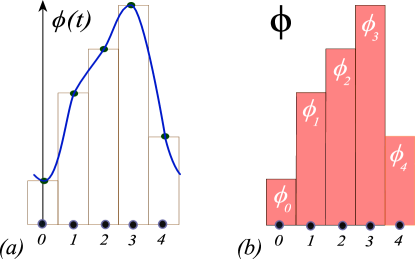
Figure 2: (Color online)    Discretization of a 1-dimensional field theory. Horizontal: $t$ coordinate, with lattice sites marked by dots and labelled by $t\in\mathbb{Z}$. (a) A periodic field $\phi(t)$, plotted as a function of continuous coordinate $t$. (b) A corresponding discretized period-$5$ Bravais cell lattice state $\mathsf{\Phi}={\overline{\phi_{0}\phi_{1}\phi_{2}\phi_{3}\phi_{4}}}$, with discretized field $\phi_{t}$ plotted as a bar centred at lattice site $t$. In what follows we use ‘lattice units’ $a=1$. Continued in figure 6.

A scalar field $\phi(x)$ over $d$ Euclidean coordinates can be discretized by replacing the continuous space by a $d$-dimensional hypercubic integer lattice $\mathbb{Z}^{d}$, with lattice spacing $a$, and evaluating the field only on the lattice points [135, 138]

$$\phi_{z}=\phi(x)\,,\qquad\qquad x=az=\mbox{lattice point}\,,\quad z\in\mathbb{Z}^{d}\,,$$ (1)

see figure 2. A field configuration (here in one spatiotemporal dimension)

$$\mathsf{\Phi}=\cdots{\phi}_{-3}{\phi}_{-2}\,{\phi}_{-1}\,{\phi}_{0}\,{\phi}_{1}{\phi}_{2}{\phi}_{3}{\phi}_{4}\cdots\,,$$ (2)

takes any set of values $\phi_{z}\in\mathbb{R}$ in system’s $\infty$-dimensional state space. A periodic field configuration $\mathsf{\Phi}$ satisfies

$$\mathsf{\Phi}({x}+{R})=\mathsf{\Phi}({x})$$ (3)

for any discrete translation $R$ in the Bravais lattice

$$\mathcal{L}=\Big{\{}\sum_{i=1}^{d}{n_{i}}{\bf a}_{i}\;|\;{n_{i}}\in\mathbb{Z}\Big{\}}$$ (4)

where the $d$ independent integer lattice vectors $\{{\bf a}_{1},{\bf a}_{2},\cdots,{\bf a}_{d}\}$ define a Bravais cell.

A field configuration occurs with probability density

$$p(\mathsf{\Phi})\,=\,\frac{1}{Z}\,\rme^{-S[\mathsf{\Phi}]}\,,\qquad Z=Z[0]\,.$$ (5)

Here $Z$ is a normalization factor, given by the partition function, the integral over probabilities of all configurations,

$$Z[\mathsf{J}]\,=\,\int d\mathsf{\Phi}\,e^{-S[\mathsf{\Phi}]+\mathsf{\Phi}\cdot\mathsf{J}}\,,\qquad d\mathsf{\Phi}=\prod_{z}^{\mathcal{L}}d\phi_{z}\,,$$ (6)

where $\mathsf{J}=\{{j}_{z}\}$ is an external source ${j}_{z}$ that one can vary site by site, and $S[\mathsf{\Phi}]$ is the action that defines the theory (discussed in more detail in section 4). The dimension of the partition function integral equals the number of lattice sites $N_{\mathcal{L}}$.

Motivated by WKB semi-classical, saddle-point approximations [98] to the partition function (6), in this paper we describe their deterministic underpinning, the corresponding deterministic field theory, with partition function built from solutions to the variational saddle-point condition

$$F[\mathsf{\Phi}_{c}]_{z}=\frac{\delta{S[\mathsf{\Phi}_{c}]}}{\delta\phi_{z}~{}}=0\,,$$ (7)

with a global deterministic solution $\mathsf{\Phi}_{c}$ satisfying this local extremal condition on every lattice site. We shall refer to the defining condition (7) as system’s ‘Euler–Lagrange equation’, keeping in mind that the field theories studied here might have a Lagrangian formulation (for example, scalar $\phi^{k}$ field theories of section 4), or be dissipative (for example, temporal Bernoulli, spatiotemporal Hénon for non-area preserving parameter values, Kuramoto-Sivashinsky or Navier-Stokes equations).

In order to distinguish a solution to the Euler–Lagrange equations (7) from an arbitrary field configuration (2), we refer to the solutions as lattice states, each a set of lattice site field values

$$\mathsf{\Phi}_{c}=\{\phi_{c,z}\}\,,$$ (8)

that satisfies the condition (7) globally, over all lattice sites. For a finite lattice $\mathcal{L}$ one needs to specify the boundary conditions (bc’s). The companion article [96] tackles the Dirichlet bc’s, a difficult, time-translation symmetry breaking, and from the periodic orbit theory perspective, a wholly unnecessary, self-inflicted pain. All that one needs to solve a field theory are the ${n}$-periodic, time-translation enforced bc’s that we shall use here.

An example is the 1 spatiotemporal dimension block of fields of period ${n}=5$ Bravais cell sketched in figure 2 (b),

$$\mathsf{\Phi}_{c}=\phi_{0}\phi_{1}\phi_{2}\phi_{3}\phi_{4}\,,$$ (9)

with its infinite repetition sketched in figure 7 (1). The first field value $\phi_{0}$ in the block is evaluated on the lattice site 0, the second $\phi_{1}$ on the lattice site 1, the $({n}+1)$th $\phi_{{n}}=\phi_{0}$ on the lattice site ${n}$, with $k$th lattice site field value $\phi_{k}=\phi_{\ell}$, where $\ell=k$ (mod ${n}$).

What we call here a chaotic ‘field’ at a discretized spacetime lattice site $z$, a solid state physicist would call a ‘particle’ at crystal site $z$, coupled to its nearest neighbors. A solid state physicist endeavours to understand $N$-particle chaotic systems in many-body or ‘large $N$’ settings, where in practice $N$ not much larger than 2 can be ‘large’. Chaotic field theory is ab initio formulated for infinite time and infinite space lattice, but its periodic theory description is -thanks to hyperbolicity– often accurate already for $N=2,3,\cdots$, where $N$ is the number of sites in a Bravais cell that tiles the spacetime.

Each lattice state is a distinct deterministic solution $\mathsf{\Phi}_{c}$ to the discretized Euler–Lagrange equations (7), so its probability density is a $N_{\mathcal{L}}$-dimensional Dirac delta function (that’s what we mean by the system being deterministic), a delta function per site ensuring that Euler–Lagrange equation (7) is satisfied everywhere,

$$p_{c}(\mathsf{\Phi})\,=\,\frac{1}{Z}\,\delta(F[\mathsf{\Phi}])\,,\qquad\mathsf{\Phi}\in\mathcal{M}_{c}\,,$$ (10)

where $\mathcal{M}_{c}$ is a small neighborhood of lattice state $\mathsf{\Phi}_{c}$. In section 7 we verify that this definition agrees with the forward-in-time Perron-Frobenius probability density evolution [54]. However, we find field-theoretical formulation vastly preferable to the forward-in-time formulation, especially when it comes to higher spatiotemporal dimensions [58].

As is case for a WKB approximation [98], the deterministic field theory partition sum has support only on lattice field values that are solutions to the Euler–Lagrange equations (7), and the partition function (5) is now a sum over configuration state space (2) points, what in theory of dynamical systems is called the ‘deterministic trace formula’ [53],

$$Z[0]=\sum_{c}\int_{\mathcal{M}_{c}}\!\!\!\!\!d\mathsf{\Phi}\,\delta(F[\mathsf{\Phi}])=\sum_{c}\frac{1}{\left|\mbox{\rm Det}\,{\mathcal{J}}_{c}\right|}\,,$$ (11)

and we refer to the $[N_{\mathcal{L}}\!\times\!N_{\mathcal{L}}]$ matrix of second derivatives

$$({\mathcal{J}}_{c})_{z^{\prime}z}=\frac{\delta F_{z^{\prime}}[\mathsf{\Phi}_{c}]}{\delta\phi_{z}}=S[\mathsf{\Phi}_{c}]_{z^{\prime}z}$$ (12)

as the orbit Jacobian matrix, and to its determinant $\mbox{\rm Det}\,{\mathcal{J}}_{c}$ as the Hill determinant. Support being on state space points means that we do not need to worry about potentials being even or odd (thus unbounded), or the system being energy conserving or dissipative, as long as its nonwandering lattice states $\mathsf{\Phi}_{c}$ set is bounded in state space. In what follows, we shall deal only with deterministic field theory and mostly omit the subscript ‘$c$’ in $\mathsf{\Phi}_{c}$.

How is a deterministic chaotic field theory different from a conventional field theory? By “spontaneous breaking of the symmetry” in a conventional theory one means that a solution does not satisfy a symmetry such as $\phi\rightarrow-\phi$; we always work in the “broken-symmetry” regime, as almost every ‘turbulent’, spatiotemporally chaotic deterministic solution breaks all symmetries. We work ‘beyond perturbation theory’, in the anti-integrable, strong coupling regime, in contrast to much of the literature that focuses on weak coupling expansions around a ‘ground state’. And, in contrast to [186, 131, 95, 14, 160], our ‘far from equilibrium’ field theory has no added dissipation, and is not driven by external noise. All chaoticity is due to the intrinsic unstable deterministic dynamics, and our trace formulas (11) are exact, not merely saddle points approximations to the exact theory.

1.1 Lattice Laplacian

Lattice free field theory is defined by action [162]

$$S_{0}[\mathsf{\Phi}]=\frac{1}{2}{\mathsf{\Phi}}{}^{\top}\left(-\Box+{\mu}^{2}\mathsf{1}\right)\mathsf{\Phi}\,,$$ (13)

where the ‘discrete Laplace operator’, ‘central difference operator’, or the ‘graph Laplacian’ [149, 156, 41, 136, 88, 157]

$$\Box\,\phi_{z}=\sum_{||z^{\prime}-z||=1}\!\!(\phi_{z^{\prime}}-\phi_{z})\quad\mbox{for all}\ z,z^{\prime}\in\mathcal{L}$$ (14)

is the average of the lattice field variation $\phi_{z^{\prime}}-\phi_{z}$ over the sites nearest to the site $z$. For example, for a hypercubic lattice in one and two dimensions this discretized Laplacian is given by

$$\Box\,\phi_{t} = \phi_{t+1}-2\,\phi_{t}+\phi_{t-1}$$ (15)

$$\Box\,\phi_{j,t} = \phi_{j,t+1}+\phi_{j+1,t}-4\,\phi_{j,t}+\phi_{j,t-1}+\phi_{j-1,t}\,.$$ (16)

For the free field theory action (13) the Euler–Lagrange equation (7) is the discretized screened Poisson equation [80], also known as the Yukawa or Klein–Gordon equation, where ${\mu}^{2}>0$ is the Klein–Gordon mass-squared.

1.2 1-dimensional lattice field theories

Discrete time evolution is frequently recast into a 1-dimensional temporal lattice field theory form, by anyone who rewrites a dynamical systems discrete time evolution problem as a $k$-term recurrence, for example in [79, 55, 56, 60]. As already in one spatiotemporal dimension there is much to be learned about the role symmetries play in solving lattice field theories, that is what we will focus on in this paper (time-reversal sections 9 and 11), with $2$-dimensional spatiotemporal field theories studied in the sequel [58].

We start with the first order difference equation that we call ‘temporal Bernoulli’ (section 2),

$$-\phi_{t+1}+({s}\phi_{t}-{m_{t}})\;\; = 0$$ (17)

in order to motivate the 2-component field formulation (251) of second-order difference Euler–Lagrange equations (51) that we call, in the cases considered here, the ‘temporal cat’ (section 3.2), ‘temporal $\phi^{3}$ theory’ (section 4.1), and ‘temporal $\phi^{4}$ theory’ (section 4.2), respectively:

$$-\phi_{t+1}+2\,\phi_{t}-\phi_{t-1}\;+\;{\mu^{2}}\phi_{t}-{m_{t}} = 0$$ (18)

$$-\phi_{t+1}+2\,\phi_{t}-\phi_{t-1}\;+\;\mu^{2}\,({1}/{4}-\phi_{t}^{2}) = 0$$ (19)

$$-\phi_{t+1}+2\,\phi_{t}-\phi_{t-1}\;+\;\mu^{2}(\phi_{t}-\,\phi_{t}^{3}) = 0\,.$$ (20)

Qualifier ‘temporal’ is used here to emphasize that we view 1-dimensional examples as special cases of ‘spatiotemporal’ field theories; much of our methodology for $d$-dimensional deterministic field theories can be profitably explained by working out $1$-dimensional field theories. Lurking here is the totality of the map-iteration dynamical systems theory, but the reader will find it more profitable, and less confusing, to think of these simply as lattice problems, and forget that the subscript $t$ often stands for ‘time’.

So, what is a ‘chaotic’, or ‘turbulent’ field theory? As we shall see in section 10, all of the above, as well as their higher-dimensional spatiotemporal siblings are ‘chaotic’ for sufficiently large ‘stretching parameter’ ${s}$, or ‘Klein-Gordon mass’ ${\mu^{2}}$. Our goal here is to make this ‘spatiotemporal chaos’ tangible and precise, by acquainting the reader what we believe are some of the simplest examples of chaotic field theories.

2 A fair coin toss

The very simplest example of a deterministic law of evolution that gives rise to ‘chaos’ is the Bernoulli map, figure 3 (a), which models a coin toss. Starting with a random initial state, the map generates, deterministically, a sequence of tails and heads with 50-50% probability.

We introduce the model in its conventional, time-evolution dynamical formulation, than reformulate it as a lattice field theory, solved by enumeration of all admissible lattice states, field configurations that satisfy a global fixed point condition, and use this simple setting to motivate (1) the fundamental fact: for a given lattice period, the Hill determinant of stabilities of global solutions counts their number (section 8.1), and (2) the topological zeta function counts their translational symmetry group orbits (section 8.2).

2.1 Bernoulli map

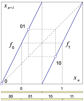
(a)     (b)

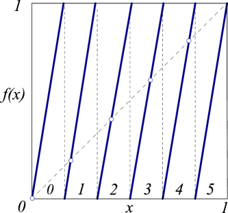
Figure 3: (Color online)    (a) The ‘coin toss’ map (21), together with the ${\overline{0}}$ fixed point, and the $\overline{01}$ 2-cycle. Preimages of the critical point $x_{c}=1/2$ partition the unit interval into $\{\mathcal{M}_{0},\mathcal{M}_{1}\}$, $\{\mathcal{M}_{00},\mathcal{M}_{01},\mathcal{M}_{10},\mathcal{M}_{11}\}$, $\dots$, subintervals. (b) The base-${s}$ Bernoulli map, here with the ‘dice throw’ stretching parameter ${s}=6$, partitions the unit interval into $6$ subintervals $\{\mathcal{M}_{{m}}\}$, labeled by the ${6}$-letter alphabet (25). As the map is a circle map, $x_{5}=1=0=x_{0}\quad(\mbox{mod}\;1)$.

The base-2 Bernoulli shift map,

$$x_{t+1}=\left\{\begin{array}[]{ll}f_{0}(x_{t})=2x_{t}\,,&x_{t}\in\mathcal{M}_{0}=[0,1/2)\\ f_{1}(x_{t})=2x_{t}\;\;(\mbox{mod}\;1)\,,&x_{t}\in\mathcal{M}_{1}=[1/2,1)\end{array}\right.\,,$$ (21)

is shown in figure 3 (a). If the linear part of such map has an integer-valued slope, or ‘stretching’ parameter $s\geq 2$,

$$x_{t+1}\,=\,{s}x_{t}$$ (22)

that maps state $x_{t}$ into a state in the ‘extended state space’, outside the unit interval, the $(\mbox{mod}\;1)$ operation results in the base-${s}$ Bernoulli circle map,

$$\phi_{t+1}={s}\phi_{t}\;\;(\mbox{mod}\;1)\,,$$ (23)

sketched as a dice throw in figure 3 (b). The $(\mbox{mod}\;1)$ operation subtracts ${m_{t}}=\left\lfloor{s}\phi_{t}\right\rfloor$, the integer part of ${s}\phi_{t}$, or the circle map winding number, to keep $\phi_{t+1}$ in the unit interval $[0,1)$, and partitions the unit interval into ${s}$ subintervals $\{\mathcal{M}_{m}\}$,

$$\phi_{t+1}={s}\phi_{t}-{m_{t}}\,,\qquad\phi_{t}\in\mathcal{M}_{{m_{t}}}\,,$$ (24)

where ${m_{t}}$ takes values in the ${s}$-letter alphabet

$${m}\in\mathcal{A}=\{0,1,2,\cdots,s-1\}\,.$$ (25)

The Bernoulli map is a highly instructive example of a hyperbolic dynamical system. Its symbolic dynamics is simple: the base-${s}$ expansion of the initial point $\phi_{0}$ is also its temporal itinerary, with symbols from alphabet (25) indicating that at time $t$ the orbit visits the subinterval $\mathcal{M}_{{m_{t}}}$. The map is a ‘shift’: a multiplication by ${s}$ acts on the base-${s}$ representation of $\phi_{0}=.{m_{1}}{m_{2}}{m_{3}}\cdots$ (for example, binary, if ${s}=2$) by shifting its digits,

$$\phi_{1} = f(\phi_{0})=.{m_{2}}{m_{3}}\cdots\,.$$ (26)

Periodic points can be counted by observing that the preimages of critical points $\{\phi_{c1},\phi_{c2},\cdots\phi_{c,s-1}\}$ = $\{{1}/s,{2}/s,\cdots,(s-1)/s\}$ partition the unit interval into $s^{n}$ subintervals $\{\mathcal{M}_{0},\mathcal{M}_{1},\cdots,\mathcal{M}_{s-1}\}$, $s^{2}$ subintervals $\{\mathcal{M}_{{m_{1}}{m_{2}}}\}$, $\dots$, $s^{n}$ subintervals, each containing one unstable period-${n}$ periodic point $\phi_{{m_{1}}{m_{2}}\cdots{m_{{n}}}}$, with stability multiplier ${s}^{n}$, see figure 3. The Bernoulli map is a full shift, in the sense that every itinerary is admissible, with one exception: on the circle, the rightmost fixed point is the same as the fixed point at the origin, $\phi_{s-1}=\phi_{0}\quad(\mbox{mod}\;1)$, so these fixed points are identified and counted as one, see figure 3. The total number of periodic points of period ${n}$ is thus

$$N_{{n}}=s^{{n}}-1\,.$$ (27)

2.2 Temporal Bernoulli

To motivate our formulation of a spatiotemporal chaotic field theory to be developed below, we now recast the local initial value, time-evolution Bernoulli map problem as a temporal lattice fixed point condition, the problem of enumerating and determining all global solutions.

‘Temporal’ here refers to the lattice site field $\phi_{t}$ and the winding number ${m_{t}}$ taking their values on the lattice sites of a 1-dimensional temporal integer lattice $t\in\mathbb{Z}$. Over a finite lattice segment, these can be written compactly as a lattice state and the corresponding symbol block

$${\mathsf{\Phi}}{}^{\top}=(\phi_{t+1},\cdots,\phi_{t+{n}})\,,\quad{\mathsf{M}}{}^{\top}=({m_{{t+1}}},\cdots,{m_{{t+{n}}}})\,,$$ (28)

where ${(\cdots)}{}^{\top}$ denotes a transpose. The Bernoulli equation (24), rewritten as a first-order difference equation

$$-\phi_{t+1}+({s}\phi_{t}-{m_{t}})=0\,,\qquad\phi_{t}\in[0,1)\,,$$ (29)

takes the matrix form

$${\mathcal{J}}\,\mathsf{\Phi}-\mathsf{M}=0\,,\qquad{\mathcal{J}}=-{\mathsf{r}}+{s}{\ \hbox{{\rm 1}\kern-6.19995pt\hbox{\rm 1}}}\,,$$ (30)

where the $[{n}\!\times\!{n}]$ matrix

$$\mathsf{r}_{jk}=\delta_{j+1,k}\,,\qquad\mathsf{r}=\left(\begin{array}[]{ccccc}0&1&&&\cr&0&1&&\cr&&&\ddots&\cr&&&0&1\cr 1&&&&0\end{array}\right)\,,$$ (31)

implements the shift operation (26), a cyclic permutation that translates forward-in-time lattice state $\mathsf{\Phi}$ by one site, ${(\mathsf{r}\mathsf{\Phi})}{}^{\top}=(\phi_{2},\phi_{3},\cdots,\phi_{n},\phi_{1})$. The time evolution law (24) must be of the same form for all times, so the operator $\mathsf{r}$ has to be time-translation invariant, with $\mathsf{r}_{{n}+1,{n}}=\mathsf{r}_{1{n}}=1$ matrix element enforcing its periodicity.

As the temporal Bernoulli condition (30) is a linear relation, a given block $\mathsf{M}$, or ‘code’ in terms of alphabet (25), corresponds to a unique temporal lattice state $\mathsf{\Phi}_{\mathsf{M}}$. That is why Percival and Vivaldi [149] refer to such symbol block $\mathsf{M}$ as a linear code. The temporal Bernoulli, however, is not a linear dynamical system: as illustrated by figure 3, it is a set of piecewise-linear ${s}$-stretching maps and their compositions, one for each state space region $\mathcal{M}_{\mathsf{M}}$.

2.3 Bernoulli as a continuous time dynamical system

The discrete time derivative of a lattice configuration $\mathsf{\Phi}$ evaluated at the lattice site $t$ is given by the difference operator [75]

$$\dot{\phi}_{t}=\left[\frac{\partial\mathsf{\Phi}}{\partial t}\right]_{t}=\frac{\phi_{t+1}-\phi_{t}}{\Delta t}\,.$$ (32)

The temporal Bernoulli condition (30) can be thus viewed as forward Euler method, a time-discretized, first-order ODE dynamical system

$$\dot{\mathsf{\Phi}}\,=\,v(\mathsf{\Phi},\mathsf{M})\,,$$ (33)

where the ‘velocity’ vector field $v$ is given by

$$v(\mathsf{\Phi},\mathsf{M})\,=\,(s-1)\,\mathsf{\Phi}-\mathsf{M}\,,$$

with the time increment set to $\Delta t=1$, and perturbations that grow (or decay) with rate $({s}-1)$. By inspection of figure 3 (a), it is clear that for shrinking, ${s}<1$ parameter values the orbit is stable forward-in-time, with a single linear branch, 1-letter alphabet $\mathcal{A}=\{0\}$, and the only lattice states being the single fixed point $\phi_{0}=0$, and its repeats $\mathsf{\Phi}=(0,0,\cdots,0)$. However, for stretching, ${s}>1$ parameter values, the Bernoulli system (more generally, Rényi’s beta transformations [159]) that we study here, every lattice state $\mathsf{\Phi}_{\mathsf{M}}$ is unstable, and there is a lattice state for each admissible symbol block $\mathsf{M}$.

A fair coin toss, summarized.

We refer to the global temporal lattice condition (30) as the ‘temporal Bernoulli’, in order to distinguish it from the 1-time step Bernoulli evolution map (23), in preparation for the study of spatiotemporal systems to be undertaken in [58]. In the lattice formulation, a global temporal lattice state $\mathsf{\Phi}_{\mathsf{M}}$ is determined by the requirement that the local temporal lattice condition (29) is satisfied at every lattice site. In spatiotemporal formulation there is no need for forward-in-time, close recurrence searches for the returning periodic points. Instead, one determines each global temporal lattice state $\mathsf{\Phi}_{\mathsf{M}}$ at one go, by solving the fixed point condition (7). The most importantly for what follows, the spatiotemporal field theory of [58], this calculation requires no recourse to any explicit coordinatization and partitioning of system’s state space.

3 A kicked rotor

Temporal Bernoulli is the simplest example of a chaotic lattice field theory. Our next task is to formulate a deterministic spatiotemporally chaotic field theory, Hamiltonian and energy conserving, because (a) that is physics, and (b) one cannot do quantum theory without it. We need a system as simple as the Bernoulli map, but mechanical. So, we move on from running in circles, to a mechanical rotor to kick.

The 1-degree of freedom maps that describe kicked rotors subject to discrete time sequences of angle-dependent force pulses $P(q_{t})$, $t\in\mathbb{Z}$,

$$q_{t+1} = q_{t}+p_{t+1}\qquad(\mbox{mod}\;1),$$ (34)

$$p_{t+1} = p_{t}+P(q_{t})\,,$$ (35)

with $2\pi q$ the angle of the rotor, $p$ the momentum conjugate to the angular coordinate $q$, and the angular pulse $P(q_{t})=P(q_{t+1})=-V^{\prime}(q_{t})$ lattice periodic with period $1$, play a key role in the theory of deterministic and quantum chaos in atomic physics, from the Taylor, Chirikov and Greene standard map [121, 38], to the cat maps that we turn to now. The equations are of the Hamiltonian form: eq. (34) is $\dot{q}=p/m$ in terms of discrete time derivative (32), i.e., the configuration trajectory starting at $q_{t}$ reaches $q_{t+1}=q_{t}+p_{t+1}\Delta{t}/m$ in one time step $\Delta{t}$. Eq. (35) is the time-discretized $\dot{p}=-\partial V(q)/\partial q$: at each kick the angular momentum $p_{t}$ is accelerated to $p_{t+1}$ by the force pulse $P(q_{t})\Delta{t}$, with the time step and the rotor mass set to $\Delta{t}=1$, $m=1$.

3.1 Cat map

The simplest kicked rotor is subject to force pulses $P(q)={\mu}^{2}q$ proportional to the angular displacement $q$: in that case, the map (34,35) is of form

$$\left(\begin{array}[]{c}q_{t+1}\\ p_{t+1}\end{array}\right)=\mathbb{J}\left(\begin{array}[]{c}q_{t}\\ p_{t}\end{array}\right)\quad(\mbox{mod}\;1)\,,\qquad{\mathbb{J}}=\left(\begin{array}[]{cc}{\mu}^{2}+1&1\\ {\mu}^{2}&1\end{array}\right)\,.$$ (36)

The $(\mbox{mod}\;1)$ makes the map a discontinuous ‘sawtooth,’ unless ${\mu}^{2}$ is a positive integer. The map is then a Continuous Automorphism of the Torus known as the Thom-Anosov-Arnol’d-Sinai ‘cat map’ [7, 63, 173], extensively studied as the simplest example of a chaotic Hamiltonian system.

The determinant of the one-time-step Jacobian is $\det\mathbb{J}=1$, i.e., the forward-in-time mapping is area-preserving. Let ${s}=\tr{\mathbb{J}}={\mu}^{2}+2$ be the trace of the Jacobian. For $|s|>2$ the $\mathbb{J}$ characteristic equation

$$\Lambda^{2}-{s}\Lambda+1=0\,,$$ (37)

has real roots $(\Lambda\,,\;\Lambda^{-1})$ and a positive Lyapunov exponent $\lambda>0$,

$$\Lambda=e^{\lambda}=\frac{1}{2}(s+\sqrt{(s-2)(s+2)})\,,\qquad{s}=\tr{\mathbb{J}}=\Lambda+\Lambda^{-1}\,.$$ (38)

The eigenvalues are functions of the stretching parameter $s$, and for $|s|>2$ the cat map (36) is a fully chaotic Hamiltonian dynamical system.

3.2 Temporal cat

In order to motivate our formulation of $d$-dimensional spatiotemporal chaotic field theories, to be developed in [58], we now recast the local initial value, Hamiltonian time-evolution as a global solution to the Euler–Lagrange equations.

The 2-component field at the temporal lattice site $t$, $\phi_{t}=(q_{t},p_{t})\in(0,1]\times(0,1]$ is kicked rotor’s the angular position and momentum. Hamilton’s equations (34,35) induce forward-in-time evolution on a 2-torus $(q_{t},p_{t})$ phase space. Eliminating the momentum by Hamilton’s discrete time velocity eq. (34),

$$(q_{t},p_{t})=\left(q_{t},\frac{q_{t}-q_{t-1}}{\Delta t}\right)\,,$$ (39)

setting the time step to $\Delta t=1$, and forgetting for a moment the $(\mbox{mod}\;1)$ condition, the forward-in-time Hamilton’s first order difference equations are brought to the second order difference, 3-term recurrence Euler–Lagrange equations for scalar field $\phi_{t}=q_{t}$,

$$\phi_{t+1}-2\,\phi_{t}+\phi_{t-1}+V^{\prime}(\phi_{t})\,=\,0\,.$$ (40)

But that is Newton’s Second Law: “acceleration equals force,” so Percival and Vivaldi [149] refer to this formulation as ‘Newtonian’. Here we follow Allroth [2], Mackay, Meiss, Percival, Kook & Dullin [129, 132, 130, 71, 115], and Li and Tomsovic [119] in referring to it as ‘Lagrangian’.

For the cat map (36), the Lagrangian passage (39) to the scalar field $\phi_{t}$ leads to the Percival-Vivaldi ‘two-configuration representation’ [149]

$$\left(\begin{array}[]{c}\phi_{t}\\ \phi_{t+1}\end{array}\right)=\mathbb{J}_{PV}\left(\begin{array}[]{c}\phi_{t-1}\\ \phi_{t}\end{array}\right)-\left(\begin{array}[]{c}0\\ {m_{t}}\end{array}\right)\,,\qquad{\mathbb{J}_{PV}}=\left(\begin{array}[]{cc}0&1\\ -1&s\end{array}\right),$$ (41)

with matrix $\mathbb{J}_{PV}$ acting on the 2-dimensional space of successive configuration points ${(\phi_{t-1},\phi_{t})}{}^{\top}$. As was case for the Bernoulli map (29), the cat map $(\mbox{mod}\;1)$ condition (36) is enforced by integers ${m_{t}}\in\mathcal{A}$, where for a given integer stretching parameter $s$ the alphabet $\mathcal{A}$ ranges over $|\mathcal{A}|={s}\!+\!1$ possible values for ${m_{t}}$,

$$\mathcal{A}=\{\underline{1},0,\dots s\!-\!1\}\,,$$ (42)

necessary to keep $\phi_{t}$ for all times $t$ within the unit interval $[0,1)$. (We find it convenient to have symbol $\underline{{m}}{}_{t}$ denote ${m_{t}}$ with the negative sign, i.e., ‘$\underline{1}$’ stands for symbol ‘$-1$’.)

Written out as a second-order difference equation, the Percival-Vivaldi map (41) takes a particularly elegant form, that we shall refer to as the temporal cat (18),

$$-\phi_{t+1}+({s}\,\phi_{t}-{m_{t}})-\phi_{t-1}=0\,,$$ (43)

or, in terms of a lattice state $\mathsf{\Phi}$, the corresponding symbol block $\mathsf{M}$ (28), and the $[{n}\!\times\!{n}]$ time translation operator $\mathsf{r}$ (31),

$$(-\mathsf{r}+s{\ \hbox{{\rm 1}\kern-6.19995pt\hbox{\rm 1}}}-\mathsf{r}^{-1})\,\mathsf{\Phi}=\mathsf{M}\,,$$ (44)

very much like the temporal Bernoulli condition (30), with the winding numbers $\mathsf{M}$ taking their values on the lattice sites of a 1-dimensional temporal lattice $t\in\mathbb{Z}$.

As was the case for temporal Bernoulli (30), the condition (41) is a linear relation: a given ‘code’ $\{{m_{t}}\}$ in terms of alphabet (42) corresponds to a unique temporal sequence $\{\phi_{t}\}$. That is why Percival and Vivaldi [149] refer to such symbol block $\mathsf{M}$ as a linear code. As for the Bernoulli system, ${m_{t}}$ can also be interpreted as ‘winding numbers’ [113], or, as they shepherd stray points back into the unit torus, as ‘stabilising impulses’ [149]. The cat map, however, is not a linear dynamical system: it is a set of piecewise-linear maps and their convolutions, one for each state space region $\mathcal{M}_{\mathsf{M}}$.

The lattice formulation (43) lends itself immediately to $d$-dimensional generalizations. An example is the Gutkin and Osipov [97] spatiotemporal cat in $d=2$ dimensions [58], an Arnold cat map-inspired Euclidean scalar field theory of form (13) for which the Euler–Lagrange equation (7) is a 5-term recurrence relation

$$-\phi_{j,t+1}-\phi_{j,t-1}+(2{s}\,\phi_{jt}-{m_{jt}})-\phi_{j+1,t}-\phi_{j-1,t}\,=\,0\,,$$ (45)

where we refer to parameter ${s}$, related to the Klein-Gordon mass in (13) by ${\mu}^{2}=d({s}-2)$, as the ‘stretching parameter’.

3.3 Temporal cat as a continuous time dynamical system

Recall that the Bernoulli first-order difference equation could be viewed as a time-discretization of the first-order linear ODE (33). The second-order difference equation (43) can be interpreted as the second order discrete time derivative ${d^{2}}/{dt^{2}}$, or the temporal lattice Laplacian (15),

$$\Box\,\phi_{t}\equiv\phi_{t+1}-2\phi_{t}+\phi_{t-1}=(s-2)\phi_{t}-{m_{t}}\,,$$ (46)

with the time step set to $\Delta t=1$. In other words, if we include the cat map forcing pulse (35) $P(\phi_{t})=-V^{\prime}(\phi_{t})=(s-2)\,\phi-{m_{t}}$ into the definition of the on-site potential, the force is linear in the angular displacement $\phi$, so the temporal cat Euler–Lagrange equation takes form (see free action (13))

$$(-\Box+{\mu}^{2}{\ \hbox{{\rm 1}\kern-6.19995pt\hbox{\rm 1}}})\,\mathsf{\Phi}=\mathsf{M}\,,$$ (47)

where the Klein-Gordon mass ${\mu}$ is related to the cat-map stretching parameter ${s}$ by ${\mu}^{2}={s}-2$.

Here we study the strong stretching, $s>2$ case, known as the discrete screened Poisson equation [69, 89, 105, 106, 80, 157], whose solutions are hyperbolic. We refer to the Euler–Lagrange equation (47) as the ‘temporal cat’, both to distinguish it from the forward-in-time Hamiltonian cat map (36), and in the anticipation of the spatiotemporal cat to be discussed in the sequel [58]. The field $\phi_{t}$ compactification to unit circle makes the spatiotemporal cat a strongly nonlinear deterministic field theory, with nontrivial symbolic dynamics.

Temporal cat, summarized.

In the spatiotemporal formulation a global temporal lattice state

$${\mathsf{\Phi}}{}^{\top}=(\phi_{t},\phi_{t+1},\cdots,\phi_{t+k})$$ (48)

is not determined by a forward-in-time ‘cat map’ evolution (36), but rather by the fixed point condition (7) that the local, 3-term discrete temporal lattice Euler–Lagrange equations (43) are satisfied at every lattice point. This temporal 1-dimensional lattice reformulation is the bridge that takes us from the single cat map (36) to the higher–dimensional coupled “multi-cat” spatiotemporal lattices [97, 96, 58].

4 Nonlinear field theories

The ‘mod 1’ in the definition of the ‘linear’ kicked rotor, makes the cat map (36) a highly nonlinear, discontinuous map. In contrast, discretized scalar $d$-dimensional Euclidean $\phi^{k}$ theories [137] are defined by smooth, polynomial actions (6) given as lattice sums over the Lagrangian density

$$S[\mathsf{\Phi}]=\sum_{z}\left\{\frac{1}{2}\sum_{\mu=1}^{d}(\partial_{\mu}\phi)_{z}^{2}+V(\phi_{z})\right\}\,,$$ (49)

with nonlinear self-interaction [185]

$$V(\phi)=\frac{\;\mu^{2}}{2}\,\phi^{2}-\frac{g}{k!}\,\phi^{k}\,,\quad k\geq 3\,,$$ (50)

where $V(\phi)$ is a local nonlinear potential [82, 72, 120, 5, 6, 4], the same for every lattice site $z$, $\mu^{2}\geq 0$ is the Klein-Gordon mass-squared, $g\geq 0$ is the strength of the self-coupling, and we set lattice constant to unity, $a=1$, throughout. The signs of the terms of (50) reflect our focus on deterministic spatiotemporal chaos, i.e., we shall study systems for whom all solutions are unstable.

The discrete Euler–Lagrange equations (7) now take form of 3-term recurrence, second-order difference equations

$$-\Box\,\phi_{z}+V^{\prime}(\phi_{z}) = 0\,.$$ (51)

4.1 A $\phi^{3}$ field theory

The simplest such nonlinear action turns out to correspond to the paradigmatic dynamicist’s model of a 2-dimensional nonlinear dynamical system, the Hénon map [101]

$$x_{t+1} = 1-a\,x_{t}^{2}+b\,y_{t}$$

$$y_{t+1} = x_{t}\,.$$ (52)

For the contraction parameter value $b=-1$ this is a Hamiltonian map (see (66) below).

The Hénon map is the simplest map that captures chaos that arises from the smooth stretch & fold dynamics of nonlinear return maps of flows such as Rössler [161]. Written as a 2nd-order inhomogeneous difference equation [72], (52) takes the temporal Hénon 3-term recurrence form, time-translation and time-reversal invariant Euler–Lagrange equation (19),

$$-\phi_{t+1}+({a}\,\phi_{t}^{2}-1)-\phi_{t-1}=0\,.$$ (53)

Just as the kicked rotor (34,35), the map can be interpreted as a kicked driven anaharmonic oscillator [100], with the nonlinear, cubic Biham-Wenzel [23] lattice site potential (50)

$$V(\phi)=\frac{1}{2}\,\mu^{2}\phi^{2}-\frac{1}{3!}\,g\,\phi^{3}\,,$$ (54)

giving rise to kicking pulse (35), so we refer to this field theory as $\phi^{3}$ theory. As discussed in detail in [183], one of the parameters can be rescaled away by translations and rescalings of the field $\phi$, and the Euler–Lagrange equation of the system can brought to various equivalent forms, such as the Hénon form (53), or the anti-integrable form (19),

$$\,-\,\frac{1}{d}\sum_{||z^{\prime}-z||=1}\!\!\!(\phi_{z^{\prime}}-\phi_{z})\;+\;\mu^{2}\,({1}/{4}-\phi_{t}^{2}) = 0\,.$$ (55)

For a sufficiently large ‘stretching parameter’ $a$, or ‘mass parameter’ ${\mu^{2}}$, the lattice states of this $\phi^{3}$ theory are in one-to-one correspondence to the unimodal Hénon map Smale horseshoe repeller, cleanly split into the ‘left’, positive stretching and ‘right’, negative stretching lattice site field values. A plot of this horseshoe, given in, for example, ChaosBook  Example 15.4 is helpfull in understanding that state space of deterministic solutions of strongly nonlinear field theories has fractal support. Devaney, Nitecki, Sterling and Meiss [64, 169, 170] have shown that the Hamiltonian Hénon map has a complete Smale horseshoe for ‘stretching parameter’ $a$ values above

$$a>5.699310786700\cdots\;.$$ (56)

In numerical [53] and analytic [77] calculations we fix (arbitrarily) the stretching parameter value to $a=6$, in order to guarantee that all $2^{n}$ periodic points $\phi={f^{{n}}(\phi)}$ of the Hénon map (52) exist, see table 1. The symbolic dynamics is binary, as simple as the Bernoulli map of figure 3 (a), in contrast to the temporal cat which has nontrivial pruning, see table 2.

4.2 A $\phi^{4}$ field theory

If a symmetry forbids the odd-power potentials such as (54), one starts instead with the Klein-Gordon [27, 21, 22, 29, 5] quartic potential (50)

$$V(\phi)=\frac{1}{2}\,\mu^{2}\phi^{2}-\frac{1}{4!}\,g\,\phi^{4}\,,$$ (57)

leading, after some translations and rescalings [183], to the Euler–Lagrange equation for the lattice scalar $\phi^{4}$ field theory (20),

$$\,-\,\frac{1}{d}\sum_{||z^{\prime}-z||=1}\!\!\!(\phi_{z^{\prime}}-\phi_{z})\;+\;\mu^{2}(\phi_{t}-\,\phi_{t}^{3}) = 0\,.$$ (58)

Topology of the state space of $\phi^{4}$ theory is very much like what we had learned for the unimodal Hénon map $\phi^{3}$ theory, except that the repeller set is now bimodal. As long as $\mu^{2}$ is sufficiently large, the repeller is a full 3-letter shift. Indeed, while Smale’s first horseshoe [167], his fig. 1, was unimodal, he also sketched the $\phi^{4}$ bimodal repeller, his fig. 5.

4.3 Computing lattice states for nonlinear theories

Unlike the temporal Bernoulli (17) and the temporal cat (18), for which the lattice state fixed point condition (7) is linear and easily solved, for nonlinear lattice field theories the lattice states are roots of polynomials of arbitrarily high order. While Friedland and Milnor [82], Endler and Gallas [77, 76, 77] and others [32, 168] have developed a powerful theory that yields Hénon map periodic orbits in analytic form, it would be unrealistic to demand such explicit solutions for general field theories on multi-dimensional lattices. We take a pragmatic, numerical route [183, 92], and search for the fixed-point solutions (7) starting with the deviation of an approximate trajectory from the 3-term recurrence (51), given by the lattice deviation vector

$$v_{t}=-\Box\,\phi_{t}+V^{\prime}(\phi_{t})\,,$$ (59)

and minimizing this error term by any suitable variational or optimization method, possibly in conjunction with a high-dimensional variant of the Newton method [57, 116, 92, 181, 147].

5 Forward-in-time stability

Consider a temporal lattice with a $d$-component field on each lattice site $t$, with time evolution given by a $d$-dimensional map (1st order difference equation)

$$\phi_{t}-f(\phi_{t-1})=0\,,\quad\phi_{t}=\{\phi_{t,1},\phi_{t,2},\dots,\phi_{t,d}\}\,.$$ (60)

A small deviation $\Delta\phi_{t}$ from $\phi_{t}$ satisfies the linearized equation

$$\Delta\phi_{t}-\mathbb{J}_{t-1}\,\Delta\phi_{t-1}=0\,,\qquad(\mathbb{J}_{t})_{ij}=\frac{\partial f(\phi_{t})_{i}}{\partial\phi_{t,j}}\,,$$ (61)

where $\mathbb{J}_{t}=\mathbb{J}(\phi_{t})$ is the 1-time step $[d\!\times\!{d}]$ Jacobian matrix, evaluated on lattice site $t$. The formula for the linearization of ${n}$th iterate of the map

$$\mathbb{J}^{n}=\mathbb{J}_{{n}-1}\mathbb{J}_{{n}-2}\cdots\mathbb{J}_{1}\mathbb{J}_{0}$$ (62)

in terms of 1-time step Jacobian matrix (61) follows by chain rule for iterated functions. For a period-$n$ Bravais cell lattice state $\mathsf{\Phi}_{c}$ we refer to this forward-in-time $[d\!\times\!{d}]$ matrix as the Floquet (or monodromy) matrix.

If the only symmetry of the system is time translation (the map (60) is the same at all temporal lattice sites, but not invariant under a lattice reflection), a lattice state $\mathsf{\Phi}_{p}$ is prime if it is not a repeat of a shorter period lattice state. Evaluated at lattice site $t_{0}$, its Floquet matrix is

$$\mathbb{J}_{p}=\mathbb{J}_{{n_{p}}-1}\mathbb{J}_{{n_{p}}-2}\cdots\mathbb{J}_{1}\mathbb{J}_{0}\,.$$ (63)

Consider a lattice state $\mathsf{\Phi}$ which is $m$th repeat of a period-${n}$ prime lattice state $\mathsf{\Phi}_{p}$ (for a sketch, see figure 7 (1)). Due to the multiplicative structure (62) of Jacobian matrices, the Floquet matrix for the $m$th repeat of a prime period-${n}$ lattice state $\mathsf{\Phi}_{p}$ is

$$\mathbb{J}^{m{n}}(\phi_{0})=\mathbb{J}^{n}(\phi_{(m-1){n}})\cdots\mathbb{J}^{n}(\phi_{n})\mathbb{J}^{n}(\phi_{0})=\mathbb{J}_{p}^{m}\,.$$ (64)

Hence it suffices to restrict our considerations to the Floquet matrix of prime lattice states.

For example, for the Hamiltonian, $b=-1$ Hénon map (52), the 1-time step Jacobian matrix (61) is

$$\mathbb{J}_{t}=\left(\begin{array}[]{cc}-2a\,\phi_{t}&-1\\ 1&0\end{array}\right)\,,\qquad(\phi_{t},\varphi_{t})=f^{t}(\phi_{0},\varphi_{0})\,.$$ (65)

So, once we have a determined a temporal Hénon lattice state $\mathsf{\Phi}_{p}$, we have its Floquet matrix $\mathbb{J}_{p}$. When $\mathbb{J}_{p}$ is hyperbolic, only the expanding eigenvalue $\Lambda_{1}=1/\Lambda_{2}$ needs to be determined, as the determinant of the Hénon 1-time step Jacobian matrix (65) is unity,

$$\det\mathbb{J}_{p}=\Lambda_{1}\Lambda_{2}=1\,.$$ (66)

The map is Hamiltonian in the sense that it preserves areas in the $[\phi,\varphi]$ plane.

6 Orbit stability

The discretized Euler–Lagrange $F[\mathsf{\Phi}_{c}]=0$ fixed point condition (7) is central to the theory of robust global methods for finding periodic orbits. In global multi-shooting, collocation [68, 90, 39], and Lindstedt-Poincaré [178, 179, 180] searches for periodic orbits, one discretizes a periodic orbit into ${n}$ sites temporal lattice configuration [57, 116, 67, 66], and lists the field value at a point of each segment

$${\mathsf{\Phi}}{}^{\top}=(\phi_{0},\phi_{1},\cdots,\phi_{{n}-1})\,.$$ (67)

Starting with an initial guess for $\mathsf{\Phi}$, a zero of function $F[\mathsf{\Phi}_{c}]$ can then be found by Newton iteration, which requires an evaluation of the $[{n}\!\times\!{n}]$ orbit Jacobian matrix

$${\mathcal{J}}_{tt^{\prime}}=\frac{\delta F[\mathsf{\Phi}_{c}]_{t}}{\delta\phi_{t^{\prime}}}\,.$$ (68)

The temporal Bernoulli condition (30) and the temporal cat discretized Euler–Lagrange equation (44) can be viewed as searches for zeros of the vector of ${n}$ functions

$$F[\mathsf{\Phi}_{\mathsf{M}}] = {\mathcal{J}}\mathsf{\Phi}-\mathsf{M}=0$$ (71)

$$\mbox{temporal Bernoulli: }\qquad{\mathcal{J}}=-{\mathsf{r}}+{s}{\ \hbox{{\rm 1}\kern-6.19995pt\hbox{\rm 1}}}$$

$$\mbox{temporal cat: }\qquad\qquad\;\;\,{\mathcal{J}}=-\mathsf{r}+s{\ \hbox{{\rm 1}\kern-6.19995pt\hbox{\rm 1}}}-\mathsf{r}^{-1}\,,$$

with the entire periodic lattice state ${\mathsf{\Phi}}_{\mathsf{M}}$ treated as a single fixed point $(\phi_{0},\phi_{1},\cdots,\phi_{{n}-1})$ in the $n$-dimensional state space unit hypercube $\mathsf{\Phi}\in[0,1)^{n}$.

For uniform stretching systems, such as the temporal Bernoulli and the temporal cat, $[{n}\!\times\!{n}]$ orbit Jacobian matrix ${\mathcal{J}}$ is a circulant, time-translation invariant matrix. Written out as matrices they are, respectively, temporal Bernoulli (71)

$${\mathcal{J}}\;\;=\;\;\left(\begin{array}[]{ccccccc}{s}&-1&0&0&\dots&0&0\\ 0&{s}&-1&0&\dots&0&0\\ 0&0&{s}&-1&\dots&0&0\\ \vdots&\vdots&\vdots&\vdots&\ddots&\vdots&\vdots\\ 0&0&0&0&\dots&{s}&-1\\ -1&0&0&0&\dots&0&{s}\end{array}\right)\,,$$ (72)

and temporal cat (71)

$${\mathcal{J}}\;\;=\;\;\left(\begin{array}[]{ccccccc}{s}&-1&0&0&\dots&0&-1\\ -1&{s}&-1&0&\dots&0&0\\ 0&-1&{s}&-1&\dots&0&0\\ \vdots&\vdots&\vdots&\vdots&\ddots&\vdots&\vdots\\ 0&0&0&0&\dots&{s}&-1\\ -1&0&0&0&\dots&-1&{s}\end{array}\right)\,.$$ (73)

While in Lagrangian mechanics matrices such as (73) are often called “Hessian”, here we refer to them collectively as ‘orbit Jacobian matrices’, to emphasize that they describe the stability of any dynamical system, be it energy-conserving, or a dissipative system without a Lagrangian formulation.

Solutions of a nonlinear field theory, such as the lattice state sketched in figure 2 (b), are in general not translation invariant, so the orbit Jacobian matrix (68) (or the ‘discrete Schrödinger operator’ [28, 166])

$${\mathcal{J}}_{c}=\left(\begin{array}[]{ccccccc}{s}_{0}&-1&0&0&\cdots&0&-1\\ -1&{s}_{1}&-1&0&\cdots&0&0\\ 0&-1&{s}_{2}&-1&\cdots&0&0\\ \vdots&\vdots&\vdots&\vdots&\ddots&\vdots&\vdots\\ 0&0&0&0&\cdots&{s}_{{n}-2}&-1\\ -1&0&0&0&\cdots&-1&{s}_{{n}-1}\end{array}\right)$$ (74)

is not a circulant matrix: each lattice state $\mathsf{\Phi}_{c}$ has its own orbit Jacobian matrix ${\mathcal{J}}_{c}={\mathcal{J}}[\mathsf{\Phi}_{c}]$, with the ‘stretching factor’ ${s}_{t}=V^{\prime\prime}(\phi_{t})+2$ at the lattice site $t$ a function of the site field $\phi_{t}$.

The orbit Jacobian matrix of a period-$(m{n})$ lattice state $\mathsf{\Phi}$, which is a $m$th repeat of a period-${n}$ prime lattice state $\mathsf{\Phi}_{p}$, has a tri-diagonal block circulant matrix form that follows by inspection from (74):

$${\mathcal{J}}=\left(\begin{array}[]{ccccc}\mathbf{s}_{p}&-\mathbf{\mathsf{r}}&&&-{\mathbf{\mathsf{r}}}{}^{\top}\\ -{\mathbf{\mathsf{r}}}{}^{\top}&\mathbf{s}_{p}&-\mathbf{\mathsf{r}}&&\\ &\ddots&\ddots&\ddots&\\ &&-{\mathbf{\mathsf{r}}}{}^{\top}&\mathbf{s}_{p}&-\mathbf{\mathsf{r}}\\ -\mathbf{\mathsf{r}}&&&-{\mathbf{\mathsf{r}}}{}^{\top}&\mathbf{s}_{p}\\ \end{array}\right)\,,$$ (80)

where block matrix $\mathbf{s}_{p}$ is a $[{n}\!\times\!{n}]$ symmetric Toeplitz matrix

$$\mathbf{s}_{p} = \left(\begin{array}[]{ccccc}{s}_{0}&-1&&&0\\ -1&{s}_{1}&-1&&\\ &\ddots&\ddots&\ddots&\\ &&-1&{s}_{{n}-2}&-1\\ 0&&&-1&{s}_{{n}-1}\\ \end{array}\right)\,,\quad\mathbf{\mathsf{r}}=\left(\begin{array}[]{ccccc}0&&\cdots&&0\\ &&&&\\ &&\ddots&&\vdots\\ &&&&\\ 1&&&&0\\ \end{array}\right)\,,$$ (91)

and $\mathbf{\mathsf{r}}$ and its transpose enforce the periodic bc’s. This period-$(m{n})$ lattice state $\mathsf{\Phi}$ orbit Jacobian matrix is as translation-invariant as the temporal cat (73), but now under Bravais lattice translations by multiples of $n$. As discussed in section 9, one can visualize this lattice state as a tiling of the integer lattice $\mathbb{Z}$ by a generic lattice state field decorating a tile of length $n$. The orbit Jacobian matrix ${\mathcal{J}}$ is now a block circulant matrix which can be brought into a block diagonal form by a unitary transformation, with a repeating $[{n}\!\times\!{n}]$ block along the diagonal, see section 10.2.1.

7 Stability of an orbit vs. its time-evolution stability

The orbit Jacobian matrix ${\mathcal{J}}[\mathsf{\Phi}_{c}]_{z^{\prime}z}$ is a high–dimensional linear stability matrix for the extremum condition $F[\mathsf{\Phi}_{c}]=0$, evaluated on the lattice state $\mathsf{\Phi}_{c}$. How is the stability so computed related to the dynamical systems’ forward-in-time stability?

As we shall show now, the two notions of stability are related by Hill’s formula

$$\left|\mbox{\rm Det}\,{\mathcal{J}}_{c}\right|=\left|\det({\ \hbox{{\rm 1}\kern-6.19995pt\hbox{\rm 1}}}-\mathbb{J}_{c})\right|$$ (92)

which relates the characteristic polynomial of the forward-in-time evolution periodic orbit Floquet matrix (monodromy matrix) $\mathbb{J}_{c}$ to the determinant of the global orbit Jacobian matrix ${\mathcal{J}}_{c}$.

While first discovered in a Lagrangian setting, Hill’s formulas apply equally well to dissipative dynamical systems, from the Bernoulli map of section 2 to Navier-Stokes and Kuramoto-Sivashinsky systems [91, 93], with the Lagrangian formalism of [129, 177, 26, 115] mostly getting in the way of understanding them. We find the discrete spacetime derivations given below a good starting point to grasp their simplicity.

Why do we need them? Let’s say that an $n$-periodic $\phi_{t+{n}}=\phi_{t}$ lattice state $\mathsf{\Phi}_{c}$ is known ‘numerically exactly’, that is to say, to a high (but not infinite) precision. One way to present the solution is to list the field value $\phi_{0}$ at a single temporal lattice site $t=0$, and instruct the reader to reconstruct the rest by stepping forward in time, $\phi_{t}=f^{t}(\phi_{0})$. However, for a linearly unstable orbit a single field value $\phi_{0}$ does not suffice to present the solution, because there is always a finite ‘Lyapunov time’ horizon $t_{Lyap}$ beyond which $f^{t}(\phi_{0})$ has lost all memory of the entire lattice state $\mathsf{\Phi}_{c}$. This problem is particularly vexing in searches for ‘exact coherent structures’ embedded in turbulence, where even the shortest period solutions have to be computed to the (for a working fluid dynamicist excessive) machine precision [86, 85, 184], in order to complete the first return to the initial state. And so the “$\cdots$ sensitivity to $\cdots$” incantations of introductory chaos courses [172, 1, 146, 53, 99] bear no relation to what we actually do in practice.

In practice, instead of relaying on forward-in-time numerical integration, global methods for finding periodic orbits [39] view them as equations for the vector fields $\dot{\phi}$ on spaces of closed curves, or, as we shall see [57, 116, 96, 58, 93], on $D$-tori spacetime tilings. In numerical implementations (67) one discretizes a periodic orbit into sufficiently many short segments [68, 90, 39, 67, 66], and lists one field value for each segment $(\phi_{1},\phi_{2},\cdots,\phi_{n})\,.$ For a ${n}$-dimensional discrete time map $f$ obtained by cutting the flow by ${n}$ local Poincaré sections, with the periodic orbit now of discrete period ${n}$, every trajectory segment can be reconstructed by short time integration, and satisfies

$$\phi_{t+1}=f_{t}(\phi_{t})\,,$$ (93)

to high accuracy, as for sufficiently short times the exponential instabilities are numerically controllable. That is why a very rough, but topologically correct global guess can robustly lead to a solution that forward-in-time methods fail to find.

7.1 Hill’s formula for a 1st order difference equation

As Hill’s formula is fundamental to our formulation of the spatiotemporal chaotic field theory, we rederive it now in three ways, relying on nothing more than elementary linear algebra. Here is its first, ‘multi-shooting’ derivation (where the reader is invited to take care of the convergence of the formal series used).

Consider a temporal lattice with a $d$-component field (60). It suffices to work out a temporal period ${n}=3$ example to understand the calculation for any period. In terms of the $[3d\!\times\!3d]$ generalized (31) block shift matrix $\mathsf{r}$

$$\mathsf{r}=\left(\begin{array}[]{ccc}0&{\ \hbox{{\rm 1}\kern-6.19995pt\hbox{\rm 1}}}_{d}&0\\ 0&0&{\ \hbox{{\rm 1}\kern-6.19995pt\hbox{\rm 1}}}_{d}\\ {\ \hbox{{\rm 1}\kern-6.19995pt\hbox{\rm 1}}}_{d}&0&0\end{array}\right)\,,$$ (94)

where ${\ \hbox{{\rm 1}\kern-6.19995pt\hbox{\rm 1}}}_{d}$ is the $d$-dimensional identity matrix, the orbit Jacobian matrix (68) has a block matrix form

$${\mathcal{J}}_{c}\,=\,{\ \hbox{{\rm 1}\kern-6.19995pt\hbox{\rm 1}}}-\mathsf{r}^{-1}\mathbb{J}\,,\quad\mathbb{J}=\left(\begin{array}[]{ccc}\mathbb{J}_{0}&0&0\\ 0&\mathbb{J}_{1}&0\\ 0&0&\mathbb{J}_{2}\end{array}\right)\,,$$ (95)

where $\mathbb{J}_{t}=\mathbb{J}(\phi_{t})$ is the 1-time step $[d\!\times\!{d}]$ Jacobian matrix (61). Next, consider

$$\mathsf{r}^{-1}\mathbb{J}=\left(\begin{array}[]{ccc}0&0&\mathbb{J}_{2}\\ \mathbb{J}_{0}&0&0\\ 0&\mathbb{J}_{1}&0\end{array}\right),\;\;(\mathsf{r}^{-1}\mathbb{J})^{2}\,=\,\left(\begin{array}[]{ccc}0&\mathbb{J}_{2}\mathbb{J}_{1}&0\\ 0&0&\mathbb{J}_{0}\mathbb{J}_{2}\\ \mathbb{J}_{1}\mathbb{J}_{0}&0&0\end{array}\right)\,,$$ (96)

and note that the ${n}=3$ repeat of $\mathsf{r}^{-1}\mathbb{J}$ is block-diagonal

$$(\mathsf{r}^{-1}\mathbb{J})^{3}=\left(\begin{array}[]{ccc}\mathbb{J}_{2}\mathbb{J}_{1}\mathbb{J}_{0}&0&0\\ 0&\mathbb{J}_{0}\mathbb{J}_{2}\mathbb{J}_{1}&0\\ 0&0&\mathbb{J}_{1}\mathbb{J}_{0}\mathbb{J}_{2}\end{array}\right)\,,$$ (100)

with $[d\!\times\!{d}]$ blocks along the diagonal cyclic permutations of each other. The trace of the $[{n}d\!\times\!{n}d]$ matrix for a period ${n}$ lattice state $\mathsf{\Phi}_{c}$

$$\Tr(\mathsf{r}^{-1}\mathbb{J})^{k}=\sum_{m=1}^{\infty}\delta_{k,m{n}}\,{n}\,\tr\mathbb{J}_{c}^{m}\,,\quad\mathbb{J}_{c}=\mathbb{J}_{{n}-1}\mathbb{J}_{{n}-2}\cdots\mathbb{J}_{1}\mathbb{J}_{0}$$ (101)

is non-vanishing only if $k$ is a multiple of ${n}$, where $\mathbb{J}_{c}$ is the forward-in-time $[d\!\times\!{d}]$ Floquet matrix of the period-$n$ lattice state $\mathsf{\Phi}_{c}$, evaluated at lattice site 0. Evaluate the Hill determinant $\mbox{\rm Det}\,{\mathcal{J}}_{c}$ by expanding

$$\ln\mbox{\rm Det}\,{\mathcal{J}}_{c} = \Tr\ln({\ \hbox{{\rm 1}\kern-6.19995pt\hbox{\rm 1}}}-{\mathsf{r}}^{-1}\mathbb{J})\,=\,-\sum_{k=1}^{\infty}\frac{1}{k}\,\Tr({\mathsf{r}}^{-1}\mathbb{J})^{k}$$ (102)

$$= -\tr\sum_{m=1}^{\infty}\frac{1}{m}\mathbb{J}_{c}^{m}=\ln\det({\ \hbox{{\rm 1}\kern-6.19995pt\hbox{\rm 1}}}_{d}-\mathbb{J}_{c})\,,$$

where ‘$\Tr$, Det ’ refer to the big, $[{n}d\!\times\!{n}d]$ global matrices, while ‘$\tr$, $\det$’ refer to the small, $[d\!\times\!{d}]$ time-stepping matrices.

The orbit Jacobian matrix ${\mathcal{J}}_{c}$ evaluated on a lattice state $\mathsf{\Phi}_{c}$ that is a solution of the temporal lattice first-order difference equation (60), and the dynamical, forward-in-time Jacobian matrix $\mathbb{J}_{c}$ are thus connected by Hill’s formula (92) which relates the global orbit stability to the Floquet, forward-in-time evolution stability. This version of Hill’s formula applies to all first-order difference equations, i.e., systems whose evolution laws are first order in time.

Perhaps the simplest example of Hill’s formula is afforded by the temporal Bernoulli lattice (30). The site field $\phi_{t}$ is a scalar, so $d=1$, the 1-time step $[1\!\times\!1]$ time-evolution Jacobian matrix (61) is the same at every lattice point $t$, $\mathbb{J}_{t}={s}$, the orbit Jacobian matrix (30) is the same for all lattice states of period ${n}$, and (see section 8.1) in this case the Hill’s formula (92) counts the numbers of lattice states

$$\mbox{temporal {Bernoulli}: }\quad N_{n}=|\mbox{\rm Det}\,{\mathcal{J}}|={s}^{{n}}-1\,,$$ (103)

in agreement with the time-evolution count (27); all itineraries are allowed, except that the periodicity of $\mathsf{r}^{n}={\ \hbox{{\rm 1}\kern-6.19995pt\hbox{\rm 1}}}$ accounts for ${\overline{0}}$ and ${\overline{s\!-\!1}}$ fixed points (see figure 3) being a single periodic point.

7.2 Hill’s formula for the trace of an evolution operator

Our second derivation redoes the first, but now in the ChaosBook  evolution operator formulation of the deterministic transport of state space orbits densities [54], setting up the generalization of the time-periodic orbit theory to the spacetime-periodic orbit theory [58].

For a $d$-dimensional deterministic map (60) the Perron-Frobenius operator

$$\mathcal{L}\,\rho(\phi_{t+1})=\int_{\mathcal{M}}\!\!d^{d}\!\phi_{t}\,\mathcal{L}(\phi_{t+1},\phi_{t})\,\rho(\phi_{t})$$ (104)

maps a state space density distribution $\rho(\phi_{t})$ one step forward-in-time. Applied repeatedly, its kernel, the $d$-dimensional Dirac delta function

$$\mathcal{L}(\phi_{t+1},\phi_{t})=\delta(\phi_{t+1}-f(\phi_{t}))\,,$$ (105)

satisfies the semigroup property

$$\mathcal{L}^{2}(\phi_{t+2},\phi_{t})=\int_{\mathcal{M}}\!\!d^{d}\!\phi_{t+1}\,\mathcal{L}(\phi_{t+2},\phi_{t+1})\,\mathcal{L}(\phi_{t+1},\phi_{t})=\delta(\phi_{t+2}-f{{}^{2}}(\phi_{t}))\,.$$ (106)

The time-evolution periodic orbit theory [53] relates the long time chaotic averages to the traces of Perron-Frobenius operators

$$\tr\mathcal{L}^{n}=\int_{\mathcal{M}}\!\!d^{d}\!\phi\,\mathcal{L}^{n}(\phi,\phi)=\int_{\mathcal{M}}\!\!d^{d}\!\phi\,\delta(\phi-f^{{n}}(\phi))\,,$$ (107)

and their weighted evolution operator generalizations, with support on all deterministic period-${n}$ temporal lattice states $\phi_{c}=f^{n}(\phi_{c})$. Usually one evaluates this trace by restricting the $d$-dimensional integral over $\mathcal{M}$ to an infinitesimal open neighborhood $c$ around a lattice site field $\phi_{c,0}$,

$$\tr_{c}\mathcal{L}^{n}=\int_{c}d^{d}\!\phi_{0}\,\delta(\phi_{0}-f^{n}(\phi_{0}))=\frac{1}{\left|\det({\ \hbox{{\rm 1}\kern-6.19995pt\hbox{\rm 1}}}-\mathbb{J}_{c})\right|}\,,$$ (108)

where $\mathbb{J}_{c}$ is the forward-in-time $[d\!\times\!d]$ Floquet matrix (101) evaluated at the period-${n}$ Bravais cell temporal site field $\phi_{c,0}$.

Alternatively, one can use the group property (106) to insert integrations over all ${n}$ temporal lattice site fields, and rewrite $\mathcal{L}^{n}$ as a product of one-time-step operators $\mathcal{L}$:

$$\tr\mathcal{L}^{n} = \int d\mathsf{\Phi}\prod_{t=0}^{{n}-1}\delta(\phi_{t+1}-f(\phi_{t}))\,,\quad d\mathsf{\Phi}=\prod_{t=0}^{{n}-1}d^{d}\!\phi_{t}\,,$$ (109)

where $\phi_{{n}}=\phi_{0}$. The lattice site field $\phi_{t}$ is a $d$-component field (60), so a period-$n$ Bravais cell lattice state $\mathsf{\Phi}$ is $({n}d)$-dimensional, with the $({n}d)$-dimensional Dirac delta function of the deterministic field theory form (11),

$$\tr\mathcal{L}^{n}=\int d\mathsf{\Phi}\,\delta(\mathsf{r}\,\mathsf{\Phi}-f(\mathsf{\Phi}))\,,$$ (110)

where $\mathsf{r}$ is the cyclic $[{n}d\!\times\!{n}d]$ version of the time translation operator (94), and $f(\mathsf{\Phi})$ acts within $d$-dimensional blocks (60) along the diagonal. We recognize the argument (60) of this $({n}d)$-dimensional Dirac delta function as the Euler–Lagrange equation (7) of the system,

$$F[\mathsf{\Phi}_{c}]=\mathsf{r}\mathsf{\Phi}_{c}-f(\mathsf{\Phi}_{c})=0\,,$$

with lattice state $\mathsf{\Phi}_{c}$ satisfying the local Euler–Lagrange equation (60) lattice site by site. Now evaluate the trace by integrating over the $d$ components of the ${n}$ lattice site fields,

$$\tr_{c}\mathcal{L}^{n}=\int_{\mathcal{M}_{c}}\!\!\!d\mathsf{\Phi}\,\delta(F[\mathsf{\Phi}])=\frac{1}{\left|\mbox{\rm Det}\,{\mathcal{J}}_{c}\right|}\,,$$ (111)

where ${\mathcal{J}}_{c}={\mathcal{J}}[\mathsf{\Phi}_{c}]$ is the $[{n}d\!\times\!{n}d]$ orbit Jacobian matrix (68) of a period-${n}$ lattice state $\mathsf{\Phi}_{c}$, and $\mathcal{M}_{c}$ is an $({n}d)$-dimensional infinitesimal open neighborhood of $\mathsf{\Phi}_{c}$. By comparing the trace evaluations (108) and (111), we see that we have again proved Hill’s formula (92) for first-order, forward-in-time difference equations, this time without writing down any explicit matrices such as (95-100).

In dynamical systems theory, one often replaces higher order derivatives (for example, Euler–Lagrange equations) by multi-component fields satisfying first order equations (for example, Hamilton’s equations), and the same is true for discrete time systems, where a $k$th order difference equation is the discrete-time analogue of a $k$th order differential equation [75]. For example, the cat map and Hénon map are usually presented as discrete time evolution over a 2-component phase space (36) and (52), rather than the 3-term scalar field recurrence conditions (43) and (53).

One could compute a Hill determinant for such system using the forward-in-time Hill’s formula for the $k$-component lattice site field, with the corresponding $[k{n}\!\times\!k{n}]$ orbit Jacobian matrix determinant (111), or use the recurrence relation to reduce the dimension of the orbit Jacobian matrix. For example, in section 3.2, in passage from the Hamiltonian to the Lagrangian formulation, the $k=2$ component phase space field $(q_{t},p_{t})$ is replaced by 1 component scalar field $\phi_{t}$. And using the 1 component scalar field one can compute the $[{n}\!\times\!{n}]$ orbit Jacobian matrices such as (72-74), whose Hill determinant equals the forward-in-time $[2\!\times\!2]$ phase space $\left|\det({\ \hbox{{\rm 1}\kern-6.19995pt\hbox{\rm 1}}}-\mathbb{J}_{c})\right|$. B, our third derivation of a Hill’s formula, is an example of such relation.

8 Hill determinants

Having shown that the inverse of Hill determinant $1/|\mbox{\rm Det}\,{\mathcal{J}}_{c}|$ gives us the lattice state’s probability (10) in the deterministic partition function, our next task is to compute it. As we shall see in section 10.2, that is often best done on the reciprocal lattice. But first we show that on hypercubic lattices we can visualize a Hill determinant geometrically, as the volume of the associated fundamental parallelepiped.

8.1 Fundamental fact

Consider temporal Bernoulli and temporal cat. The orbit Jacobian matrix $\mathcal{J}$ stretches the state space unit hypercube $\mathsf{\Phi}\in[0,1)^{n}$ into the $n$-dimensional fundamental parallelepiped, and maps each periodic lattice state ${\mathsf{\Phi}}_{\mathsf{M}}$ into an integer lattice $\mathbb{Z}^{n}$ site, which is then translated by the winding numbers $\mathsf{M}$ into the origin, in order to satisfy the fixed point condition (71). Hence $N_{n}$, the total number of the solutions of the fixed point condition equals the number of integer lattice points within the fundamental parallelepiped, a number given by what Baake et al [13] call the ‘fundamental fact’,

$$N_{n}=|\mbox{\rm Det}\,{\mathcal{J}}|\,,$$ (112)

i.e., fact that the number of integer points in the fundamental parallelepiped is equal to its volume, or, what we refer to as its Hill determinant.

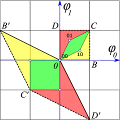
(a)         (b) 

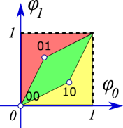
Figure 4: (Color online)    (a) The Bernoulli map (21) periodic points $\mathsf{\Phi}_{\mathsf{M}}=(\phi_{0},\phi_{1})$ of period 2 are the ${\overline{0}}=(0,0)$ fixed point, and the 2-cycle $\mathsf{\Phi}_{01}=({1}/{3},{2}/{3})$, see figure 3 (a). They all lie within the unit square $[0BCD]$, which is mapped by the orbit Jacobian matrix $-{\mathcal{J}}$ (126) into the fundamental parallelepiped $[0B^{\prime}C^{\prime}D^{\prime}]$. Periodic points $\mathsf{\Phi}_{\mathsf{M}}$ are mapped by ${\mathcal{J}}$ onto the integer lattice, ${\mathcal{J}}\mathsf{\Phi}_{\mathsf{M}}\in\mathbb{Z}^{n}$, and are sent back into the origin by integer translations $\mathsf{M}$, in order to satisfy the fixed point condition (71). Note that this fundamental parallelepiped is covered by 3 unit area quadrilaterals, hence $|\mbox{\rm Det}\,{\mathcal{J}}|=3$. (b) Conversely, in the flow conservation sum rule (136) sum over all lattice states $\mathsf{M}$ of period ${n}$, the inverse of the Hill determinant defines the ‘neighborhood’ of a lattices state as the corresponding fraction of the unit hypercube volume.

The action of the orbit Jacobian matrix ${\mathcal{J}}$ for period-2 lattice states (periodic points) of the Bernoulli map of figure 3 (a), suffices to convey the idea. In this case, the $[2\!\times\!2]$ orbit Jacobian matrix (30), the unit square basis vectors, and their images are

$${\mathcal{J}} = \left(\begin{array}[]{cc}2&-1\\ -1&2\end{array}\right)\,,$$ (115)

$$\mathsf{\Phi}^{(B)} = \left(\begin{array}[]{c}1\\ 0\end{array}\right)\;\to\;\mathsf{\Phi}^{(B^{\prime})}={\mathcal{J}}\,\mathsf{\Phi}^{(B)}=\left(\begin{array}[]{c}2\\ -1\end{array}\right)\,,$$ (120)

$$\mathsf{\Phi}^{(D)} = \left(\begin{array}[]{c}0\\ 1\end{array}\right)\;\to\;\mathsf{\Phi}^{(D^{\prime})}={\mathcal{J}}\,\mathsf{\Phi}^{(D)}=\left(\begin{array}[]{c}-1\\ 2\end{array}\right)\,,$$ (125)

i.e., the columns of the orbit Jacobian matrix are the edges of the fundamental parallelepiped,

$${\mathcal{J}}=\left(\mathsf{\Phi}^{(B^{\prime})}\mathsf{\Phi}^{(D^{\prime})}\right)\,,$$ (126)

see figure 4 (a), and $N_{2}=|\mbox{\rm Det}\,{\mathcal{J}}|=3$, in agreement with the periodic orbit count (27).

In general, the unit vectors of the state space unit hypercube $\mathsf{\Phi}\in[0,1)^{n}$ point along the $n$ axes; orbit Jacobian matrix $\mathcal{J}$ stretches them into a fundamental parallelepiped basis vectors $\mathsf{\Phi}^{(j)}$, each one a column of the $[{n}\!\times\!{n}]$ matrix

$${\mathcal{J}}=\left(\mathsf{\Phi}^{(1)}\mathsf{\Phi}^{(2)}\cdots\mathsf{\Phi}^{({n})}\right)\,.$$ (127)

The Hill determinant

$$\mbox{\rm Det}\,{\mathcal{J}}=\mbox{\rm Det}\,\!\left(\mathsf{\Phi}^{(1)}\mathsf{\Phi}^{(2)}\cdots\mathsf{\Phi}^{({n})}\right)\,,$$ (128)

is then the volume of the fundamental parallelepiped whose edges are basis vectors $\mathsf{\Phi}^{(j)}$. Note that the unit hypercubes and fundamental parallelepipeds are half-open, as indicated by dashed lines in figure 4 (a), so that their translates form a partition of the extended state space (22). For another example of fundamental parallelepipeds, see figure 5.

For temporal cat the total number of lattice states is again, as for the Bernoulli system, given by the fundamental fact (112). However, while for the temporal Bernoulli every sequence of alphabet letters (25) but one is admissible, for temporal cat the condition (43) constrains admissible winding numbers blocks $\mathsf{M}$.

For period-1, constant field lattice states $\phi_{t+1}=\phi_{t}=\phi_{t-1}$ it follows from (43) that

$$({s}-2)\phi_{t}={m_{t}}\,,$$

so the orbit Jacobian matrix is a $[1\times 1]$ matrix, and there are

$$N_{1}={s}-2$$ (129)

period-1 lattice states. This is easy to verify by counting the admissible ${m_{t}}$ values. Since $\phi_{t}\in[0,1)$, the range of $m_{t}$ is ${m_{t}}\in[0,s-2)$. So three of the (42) temporal cat  letters are not admissible: $\underline{1}$ is below the range, and $s-2$ and $s-1$ are above it.

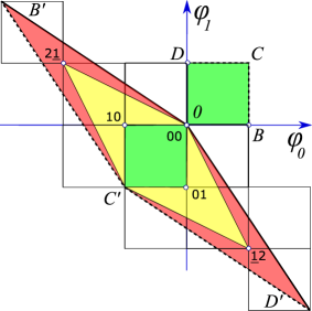
(a)      (b) 

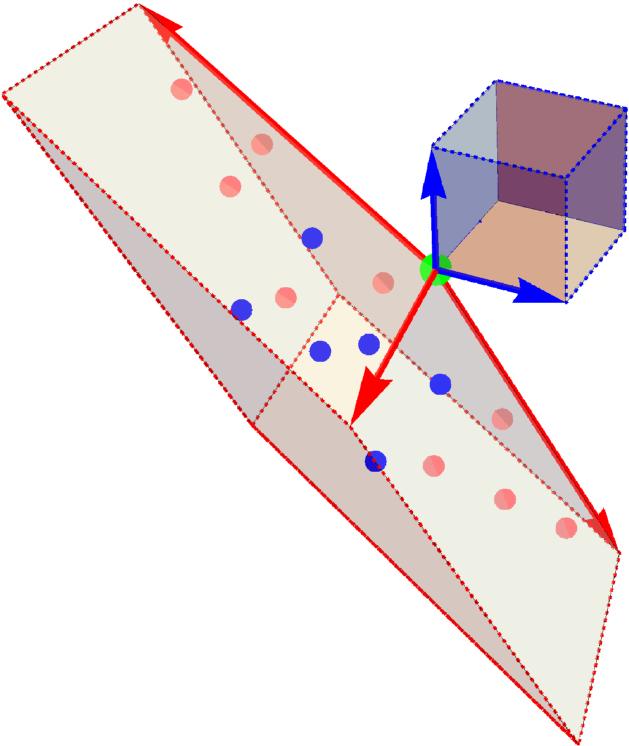
Figure 5: (Color online)    (a) For $s=3$, the temporal cat (44) has 5 period-2 lattice states $\mathsf{\Phi}_{\mathsf{M}}=(\phi_{0},\phi_{1})$: $\mathsf{\Phi}_{00}$ fixed point and period-2 lattice states $\{\mathsf{\Phi}_{01},\mathsf{\Phi}_{10}\}$, $\{\mathsf{\Phi}_{\underline{1}2},\mathsf{\Phi}_{2\underline{1}}\}$. They lie within the unit square $[0BCD]$, and are mapped by the $[2\!\times\!2]$ orbit Jacobian matrix $-{\mathcal{J}}$ (130) into the fundamental parallelepiped $[0B^{\prime}C^{\prime}D^{\prime}]$, as in, for example, Bernoulli figure 4. The images of periodic points $\mathsf{\Phi}_{\mathsf{M}}$ land on the integer lattice, and are sent back into the origin by integer translations $\mathsf{M}={m_{0}}{m_{1}}$, in order to satisfy the fixed point condition ${\mathcal{J}}\mathsf{\Phi}_{\mathsf{M}}+\mathsf{M}=0$. (b) A 3-dimensional [ blue basis vectors] unit-cube stretched by $-{\mathcal{J}}$ (131) into the [ red basis vectors] fundamental parallelepiped. For $s=3$, the temporal cat (44) has 16 period-3 lattice states: a $\mathsf{\Phi}_{000}$ fixed point at the vertex at the origin, [ pink dots] 3 period-3 orbits on the faces of the fundamental parallelepiped, and [ blue dots] 2 period-3 orbits in its interior. An $n$-dimensional state space unit hypercube $\mathsf{\Phi}\in[0,1)^{n}$ and the corresponding fundamental parallelepiped are half-open, as indicated by dashed lines, so the integer lattice points on the far corners, edges and faces do not belong to it.

The action of the temporal cat orbit Jacobian matrix can be hard to visualize, as a period-2 lattice field is a 2-torus, period-3 lattice field a 3-torus, etc.. Still, the fundamental parallelepiped for the period-2 and period-3 lattice states, figure 5, should suffice to convey the idea. The fundamental parallelepiped basis vectors are the columns of ${\mathcal{J}}$. The $[2\!\times\!2]$ orbit Jacobian matrix (73) and its Hill determinant are

$${\mathcal{J}}=\left(\begin{array}[]{cc}s&-2\\ -2&s\end{array}\right)\,,\qquad N_{2}=\mbox{\rm Det}\,{\mathcal{J}}=({s}-2)({s}+2)\,,$$ (130)

(compare with the lattice states count (285)), with the resulting fundamental parallelepiped shown in figure 5 (a). Period-3 lattice states for $s=3$ are contained in the half-open fundamental parallelepiped of figure 5 (b), defined by the columns of $[3\!\times\!3]$ orbit Jacobian matrix

$${\mathcal{J}}=\left(\begin{array}[]{ccc}{s}&-1&-1\\ -1&{s}&-1\\ -1&-1&{s}\end{array}\right)\,,\qquad N_{3}=\mbox{\rm Det}\,{\mathcal{J}}=({s}-2)({s}+1)^{2}\,,$$ (131)

again in agreement with the periodic orbit count (285). The 16 period-3, ${s}=3$ lattice states $\mathsf{\Phi}_{\mathsf{M}}=(\phi_{0},\phi_{1},\phi_{2})$ are the $\mathsf{\Phi}_{000}$ fixed point at the vertex at the origin, 3 period-3 orbits on the faces of the fundamental parallelepiped, and 2 period-3 orbits in its interior.

In this example there is no need to go further with the fundamental fact Hill determinant evaluations, as the explicit formula for the numbers of periodic lattice states is well known [108, 113]. The temporal cat equation (43) is a linear $2$nd-order inhomogeneous difference equation ($3$-term recurrence relation) with constant coefficients that can be solved by standard methods [75] that parallel the theory of linear differential equations. Inserting a solution of form $\phi_{t}=\Lambda^{t}$ into the $m_{t}$=0 homogenous $2$nd-order temporal cat condition (43) yields the characteristic equation (37) with roots $\{\Lambda\,,\;\Lambda^{-1}\}$. The result is that the number of temporal lattice states of period ${n}$ is

$$N_{{n}}=|\mbox{\rm Det}\,{\mathcal{J}}|=\Lambda^{{n}}+\Lambda^{-{n}}-2\,,$$ (132)

often written as

$$N_{n}=2\,T_{{n}}(s/2)-2\,,$$ (133)

where $T_{{n}}(s/2)$ is the Chebyshev polynomial of the first kind (this discussion continues in section 10.2).

Note that in the temporal lattice reformulation, both temporal Bernoulli and temporal cat happen to involve two distinct lattices:

• In the latticization (1) of a time continuum, one replaces a time-dependent field $\phi(t)$ at time $t\in\mathbb{R}$ of any dynamical system by a discrete set of its values $\phi_{t}=\phi(a\,t)$, at time instants $t\in\mathbb{Z}$. Here the subscript ‘$t$’ indicates a coordinate over which the field $\phi$ lives.

• A peculiarity of the temporal Bernoulli and temporal cat is that the field $\phi_{t}$, (23) and (41), is confined to the unit interval $[0,1)$, imparting an integer lattice structure onto the intermediate calculational steps in the extended state space (22) on which the orbit Jacobian matrix $\mathcal{J}$ acts. Nothing like that applies to general nonlinear field theories of section 4.

8.2 Periodic orbit theory

How come that a Hill determinant (112) counts lattice states?

For a general, nonlinear fixed point condition $F[\mathsf{\Phi}]=0$, expansion (102) in terms of traces is a cycle expansion [47, 9, 53], with support on periodic orbits. Ozorio de Almeida and Hannay [3] were the first to relate the number of periodic points to a Jacobian matrix generated volume; in 1984 they used such relation as an illustration of their ‘principle of uniformity’: “periodic points of an ergodic system, counted with their natural weighting, are uniformly dense in phase space.” In periodic orbit theory [47, 52] this principle is stated as a flow conservation sum rule, where the sum is over all lattice states $\mathsf{M}$ of period ${n}$,

$$\sum_{|\mathsf{M}|={n}}\frac{1}{|\det({\ \hbox{{\rm 1}\kern-6.19995pt\hbox{\rm 1}}}-\mathbb{J}_{\mathsf{M}})|}\;=1\,,$$ (134)

or, by Hill’s formula (92),

$$\sum_{|\mathsf{M}|={n}}\frac{1}{|\mbox{\rm Det}\,{\mathcal{J}}_{\mathsf{M}}|}\;=1\,.$$ (135)

For the Bernoulli and temporal cat systems the ‘natural weighting’ takes a particularly simple form, as the Hill determinant of the orbit Jacobian matrix is the same for all periodic points of period ${n}$, $\mbox{\rm Det}\,{\mathcal{J}}_{\mathsf{M}}=\mbox{\rm Det}\,{\mathcal{J}}$, whose number is thus given by (103). For example, the sum over the ${n}=2$ lattice states is,

$$\frac{1}{|\mbox{\rm Det}\,{\color[rgb]{0,1,0}{\mathcal{J}}_{00}}|}+\frac{1}{|\mbox{\rm Det}\,{\color[rgb]{1,0,0}{\mathcal{J}}_{01}}|}+\frac{1}{|\mbox{\rm Det}\,{\color[rgb]{1,1,0}{\mathcal{J}}_{10}}|}=1\,,$$ (136)

see figure 4 (b). Furthermore, for any piece-wise linear system all curvature corrections [50] for orbits of periods $k>{n}$ vanish, leading to explicit lattice state-counting formulas of kind reported in this paper.

In the case of temporal Bernoulli or temporal cat, the hyperbolicity is the same everywhere and does not depend on a particular solution $\mathsf{\Phi}_{c}$, counting periodic orbits is all that is needed to solve a cat-map dynamical system completely; once periodic orbits are counted, all cycle averaging formulas [51] follow.

Fritz, this is the ‘periodic orbit theory’. And if you don’t know, now you know.

9 Translations and reflections

Though this exposition is nominally about ‘evolution in time’, ‘time’ is such a loaded notion, a straightjacket hard to escape, that it is best to forget about ‘time’ for time being, and think instead like a crystallographer, about lattices and the space groups that describe their symmetries.

Of necessity, there are many group-theoretic notions a crystallographer must juggle (see ChaosBook  sect. 11.2), but only a few key things to understand. For a 1-dimensional lattice, there are only two kinds of qualitatively different symmetry transformations,

• translations (139) and reflections (141), which reverse the direction of translation.

• There are two kinds of reflections (151), across a lattice site, and across a mid-point between lattice sites, figure 6.

• While the lattice $\mathcal{L}$ and its space group $G$ are both infinite, orbits of lattice states are finite and described by finite cyclic and dihedral groups, figure 7.

• A lattice state has one of the 4 possible symmetries, figure 9. They are the building blocks of zeta functions of section 11.

Should the reader find symmetries of infinite lattices too obstruse: to understand all that one needs to know about translations and reflections, it suffices to understand the symmetries of a triangle and a square, figure 8.

9.1 Internal symmetries

In addition to the spacetime symmetries, a field theory might have an internal symmetry, a group of transformations that leaves the Euler–Lagrange equations invariant, but acts only on a lattice site field, not on the spacetime lattice.

The $\phi^{4}$ action (57) is invariant under the $\textrm{D}_{1}$ reflection $\phi_{z}\to-\phi_{z}$. The temporal Bernoulli (29) and temporal cat (43) Euler–Lagrange equations are invariant under $\textrm{D}_{1}$ inversion of the field though the center of the $0\leq\phi_{z}<1$ unit interval:

$$\bar{\phi}_{z}=1-\phi_{z}\quad\mbox{mod}\;1\,.$$ (137)

If $\mathsf{\Phi}=\{\phi_{z}\}$ is a lattice state of the system, its inversion $\bar{\mathsf{\Phi}}=\{\bar{\phi}_{z}\}$ is also a lattice state. So every lattice state of the temporal Bernoulli and the temporal cat either belongs to a pair of asymmetric lattice states $\{\mathsf{\Phi},\bar{\mathsf{\Phi}}\}$, or is symmetric under the inversion. Figures 10 and 13 illustrate such symmetries.

In principle, the internal symmetries should also be quotiented, but to keep things as simple as possible, they are not quotiented in this paper.

9.2 Symmetries of 1-dimensional lattices, sublattices

A space group $G$ is the set of all translations and rotations that puts a crystallographic structure $\mathcal{L}$ in coincidence with itself. To make the exposition as simple as possible, here we focus on 1-dimensional crystals, with sites labeled by integer lattice $\mathcal{L}=\mathbb{Z}$. Their space groups crystallographers [70] call line groups. There are only two 1-dimensional space groups $G$: $p1$, or the infinite cyclic group $\textrm{C}_{\infty}$ of all lattice translations, and $p1m$, the infinite dihedral group $\textrm{D}_{\infty}$ of all translations and reflections [114],

$$\textrm{D}_{\infty}=\{\cdots,\mathsf{r}_{-2},\mathsf{\sigma}_{-2},\mathsf{r}_{-1},\mathsf{\sigma}_{-1},1,\mathsf{\sigma},\mathsf{r}_{1},\mathsf{\sigma}_{1},\mathsf{r}_{2},\mathsf{\sigma}_{2},\cdots\}\,.$$ (138)

A half of the elements are translations (‘shifts’; for finite period lattices, ‘rotations’). $\mathsf{r}_{0}=1$ denotes the identity, and the $\mathsf{r}_{1}=\mathsf{r}$, $\mathsf{r}_{2}=\mathsf{r}^{2}$, $\cdots$, $\mathsf{r}_{k}=\mathsf{r}^{k}$, $\cdots$, denote translations by $1,2,\cdots,k,\cdots$ lattice points. They form the infinite cyclic group

$$\textrm{C}_{\infty}=\{\cdots,\mathsf{r}_{-2},\mathsf{r}_{-1},1,\mathsf{r}_{1},\mathsf{r}_{2},\mathsf{r}_{3},\cdots\}\,,$$ (139)

a subgroup of $\textrm{D}_{\infty}$, in crystallography called the translation group.

The other half of elements are reflections $\mathsf{\sigma}_{k}^{2}=1$ (‘inversions’, ‘time reversals’, ‘flips’), defined by first translating by $k$ steps, and then reflecting over the 0th lattice point, resulting in a ‘translate-reflect’ operation

$$\mathsf{\sigma}_{k}=\mathsf{\sigma}\mathsf{r}_{k}\,.$$ (140)

The defining property of translate & reflect groups (‘dihedral’ groups, ‘flip systems’ [114]) is that any reflection reverses the direction of the translation

$$\mathsf{\sigma}_{k}\mathsf{r}=\mathsf{r}^{-1}\mathsf{\sigma}_{k}\,.$$ (141)

The group multiplication (or ‘Cayley’) table for successive group actions $g_{i}g_{j}$ follows:

𝗋i𝗋i+jσj−iσiσi+j𝗋j−i.fragments fragmentsr𝑖fragmentsr𝑖𝑗fragmentsσ𝑗𝑖fragmentsσ𝑖fragmentsσ𝑖𝑗fragmentsr𝑗𝑖\begin{tabular}[]{c|cc}&$\mathsf{r}_{j}$&$\mathsf{\sigma}_{j}$\\ \hline\cr$\mathsf{r}_{i}$&$\mathsf{r}_{i+j}$&$\mathsf{\sigma}_{j-i}$\\ $\mathsf{\sigma}_{i}$&$\mathsf{\sigma}_{i+j}$&$\mathsf{r}_{j-i}$\end{tabular}\,.

rjσjrjσj (142)

Multiplication either adds up translations, or shifts and then reverses their direction. The order in which the elements $g_{i}g_{j}$ act is right to left, i.e., a group element acts on the expression to its right.

A crystallographer organizes the subgroups of a space group $G$ by means of Bravais lattices $\mathcal{L}_{\mathbf{a}}$ (4), sublattices of the lattice $\mathbb{Z}$, each defined here by a 1-dimensional Bravais cell of period $n$, given by a lattice vector $\mathbf{a}$ of integer length $n$,

$$\mathcal{L}_{\mathbf{a}}=\{j\mathbf{a}\,|\,j\in\mathbb{Z}\}\,,$$ (143)

with the lattice generated by the infinite translation group of all discrete translations replaced by

$$\mathsf{r}_{j}\to\mathsf{r}_{j\mathbf{a}}$$

multiples of $\mathbf{a}$, resulting in

$$H_{\mathbf{a}}=\{\cdots,\mathsf{r}_{-2\mathbf{a}},\mathsf{r}_{-\mathbf{a}},1,\mathsf{r}_{\mathbf{a}},\mathsf{r}_{2\mathbf{a}},\cdots\}\,,$$ (144)

infinite translation subgroup of $\textrm{C}_{\infty}$. You can visualize a lattice state invariant under subgroup $H_{\mathbf{a}}$ as a tiling of the lattice $\mathbb{Z}$ by a generic lattice state over tile of length $n$.

Another family of subgroups of $\textrm{D}_{\infty}$ is obtained by substituting elements of $\textrm{D}_{\infty}$ (138) by

$$\mathsf{r}_{j}\to\mathsf{r}_{j\mathbf{a}}\,,\qquad\mathsf{\sigma}\to\mathsf{\sigma}_{k}\quad 0\leq{k}<{n}\,,$$

resulting in ${n}$ infinite dihedral subgroups

$$H_{\mathbf{a},k}=\{\cdots,\mathsf{r}_{-2\mathbf{a}},\mathsf{\sigma}_{k}\mathsf{r}_{-2\mathbf{a}},\mathsf{r}_{-\mathbf{a}},\mathsf{\sigma}_{k}\mathsf{r}_{-\mathbf{a}},1,\mathsf{\sigma}_{k},\mathsf{r}_{\mathbf{a}},\mathsf{\sigma}_{k}\mathsf{r}_{\mathbf{a}},\mathsf{r}_{2\mathbf{a}},\mathsf{\sigma}_{k}\mathsf{r}_{2\mathbf{a}},\cdots\}\,,$$ (145)

each given by a Bravais cell of period $n$, with reflection across a symmetry point shifted $k$ half-steps, see (154).

9.3 Classes

Definition: A class is the set of elements left invariant by conjugation with all elements $g$ of the group $G$, where an element $b$ is conjugate to element $a$ if

$$b=g\,a\,g^{-1}\,.$$ (146)

By (141), a conjugation by any reflection reverses the direction of translation

$$\mathsf{\sigma}_{i}\mathsf{r}_{j}\mathsf{\sigma}_{-i}=\mathsf{r}_{-j}\,,$$ (147)

so every translation pairs up with the equal counter-translation to form

identity class $$\qquad\{1\}\,,\quad\qquad\;j=0$$ (148)

translation classes $$\qquad\{\mathsf{r}_{j},\mathsf{r}_{-j}\}\,,\quad j=1,2,3,\cdots\,.$$ (149)

The $\mathsf{r}_{0}=1$ commutes with all group elements, and is thus always a class by itself.

From the multiplication table (142) it follows that a conjugate of a reflection

$$\mathsf{r}_{i}\,\mathsf{\sigma}_{j}\mathsf{r}_{i}^{-1}=\mathsf{\sigma}_{j-2i}\,,\quad\mathsf{\sigma}_{i}\mathsf{\sigma}_{j}\mathsf{\sigma}_{i}^{-1}=\mathsf{\sigma}_{2i-j}\,.$$ (150)

is a reflection related to it by a ${2i}$ translation. Hence the even subscript reflections belong to one class, and the odd subscript reflections to the other:

even $$\quad\{\mathsf{\sigma}_{2m}\}\,,\qquad m\in\mathbb{Z}$$

odd $$\quad\{\mathsf{\sigma}_{2m+1}\}\,.$$ (151)

By (150) $rH_{{n},k}r^{-1}=H_{{n},k-2}$, so for odd $n$, all subgroups $H_{{n},k}$ are conjugate subgroups, and for even $n$, $H_{{n},k}$ separate into 2 sets of conjugate subgroups,

even $$\quad\{H_{2m,2j}\}\,,\qquad 0\leq j<m$$

odd $$\quad\{H_{2m,2j+1}\}\,,$$ (152)

each containing $m$ subgroups.

9.4 Reflections

What’s the difference between an ‘odd’ and an ‘even’ reflection? Every element in a class is equivalent to any other of its elements. So, to understand what everybody in a given class does, it suffices to work out what a single representative does: it suffices to analyse the $H_{{n},0}$ and $H_{{n},1}$ to account for all $H_{{n},k}$.

So far, we have only discussed the abstract structure of the space group $\textrm{D}_{\infty}$ and its subgroups. But the difference between an ‘odd’ and an ‘even’ is easiest to grasp by working out the action of $\mathsf{\sigma}_{k}$ on a lattice state.

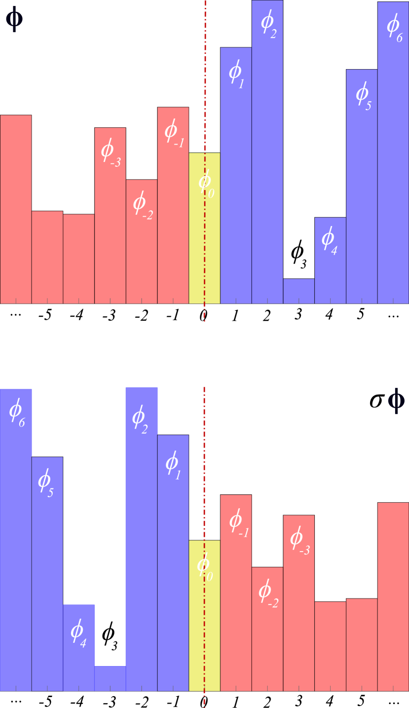
(even)

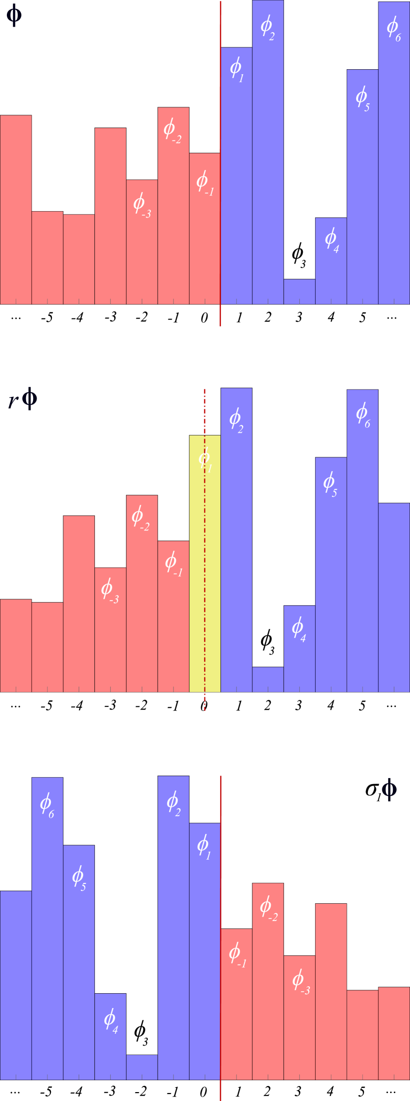
(odd)

Figure 6: (Color online)    There are two classes of lattice state reflections, even (153) and odd (154). (Even) reflection $\mathsf{\sigma}$ exchanges (blue $\phi_{j}$) $\leftrightarrow$ (red $\phi_{-j}$) marked by dashed line reflection axis, with lattice site ${0}$ fixed. (Odd) reflection $\mathsf{\sigma}_{1}=\mathsf{\sigma}\mathsf{r}$ swaps the ‘blues’ and the ‘reds’ by a lattice translation $\mathsf{\Phi}\to\mathsf{r}\mathsf{\Phi}$, followed by a reflection $\mathsf{\sigma}$. The result is a reflection across the midpoint of the [01] interval, marked by full line reflection axis. See figure 2 (b) for the notation. Continued in figure 7.

Even class.

Take $\mathsf{\sigma}=\mathsf{\sigma}_{0}$ as a representative of all even reflections $\mathsf{\sigma}_{2m}$, and act on a lattice state (8):

$$\mathsf{\Phi} = \cdots{\phi}_{-3}{\phi}_{-2}\,{\phi}_{-1}\,{\phi}_{0}\,{\phi}_{1}{\phi}_{2}{\phi}_{3}{\phi}_{4}\cdots$$

$$\mathsf{\sigma}\mathsf{\Phi} = \cdots{\phi}_{5}{\phi}_{4}{\phi}_{3}{\phi}_{2}{\phi}_{1}{\framebox{\hskip 1.2pt${\phi}_{0}$\hskip 1.2pt}}\,{\phi}_{-1}{\phi}_{-2}{\phi}_{-3}\cdots\,,$$ (153)

with  ${\phi}_{0}$  indicating that the field at the lattice site $0$ is unchanged by the reflection, see figure 6 (even).

Odd class.

Take $\mathsf{\sigma}_{1}$ as a representative of all odd reflections $\mathsf{\sigma}_{2m+1}$. The result is:

$$\mathsf{\Phi} = ~{}~{}~{}~{}\,\cdots{\phi}_{-3}{\phi}_{-2}{\phi}_{-1}\,{\underline{\phi}}{}_{0}\,\,{\phi}_{1}{\phi}_{2}{\phi}_{3}{\phi}_{4}\cdots$$

$$\mathsf{r}\mathsf{\Phi} = ~{}\,\cdots{\phi}_{-3}{\phi}_{-2}{\phi}_{-1}{\phi}_{0}\,{\underline{\phi}}{}_{1}\,\,{\phi}_{2}{\phi}_{3}{\phi}_{4}{\phi}_{5}\cdots$$

$$\mathsf{\sigma}_{1}\mathsf{\Phi}=\mathsf{\sigma}\mathsf{r}\mathsf{\Phi} = ~{}~{}~{}~{}\cdots{\phi}_{6}{\phi}_{5}{\phi}_{4}{\phi}_{3}{\phi}_{2}\,{\underline{\phi}}{}_{1}|\,{\phi}_{0}{\phi}_{-1}{\phi}_{-2}{\phi}_{-3}\cdots\,,$$ (154)

where ${\underline{\phi}}{}_{j}$ indicates the field value at the lattice site $0$, and $|$ indicates a reflection across midpoint between lattice sites $0$ and $1$, see figure 6 (odd).

More generally, one can say that the subscript $k$ in the ‘translate-reflection’ (140) operation $\mathsf{\sigma}_{k}=\mathsf{\sigma}\mathsf{r}_{k}$ advances the reflection point by $k/2$ steps, and then reflects across it.

If you do not find the two kinds of reflections intuitive, the distinction becomes crystal clear once you have a look at the smallest Bravais lattices, lattices of periods 3 and 4, figure 8.

9.5 Symmetries of a system and of its solutions

What’s the deal about classes? A ‘class’ is a refinement of our intuitive notion that “rotations are rotations, and translations are translations.” Translated into a more familiar language, conjugation (146) is central to all of physics: a ‘law’ $F(\mathsf{\Phi})$ is invariant if it retains its form in all symmetry related coordinate frames,

$$F(\mathsf{\Phi})=g^{-1}F(g\,\mathsf{\Phi})\,,$$ (155)

where $g$ is a representation of group element $g\in G$. If this holds, we say that $G$ is the symmetry of the system.

For example, the ‘temporal Bernoulli’ Euler–Lagrange equation (30) retains its form under conjugation by any $\textrm{C}_{\infty}$ translation (139),

$$\mathsf{r}_{i}({s}1-\mathsf{r}_{1})\mathsf{r}_{i}^{-1}\mathsf{\Phi}=({s}1-\mathsf{r}_{1})\mathsf{\Phi}\,,$$ (156)

while the Euler–Lagrange second-order difference equations (51), ‘temporal cat’, ‘temporal Hénon’, and ‘temporal $\phi^{4}$ theory’ Euler–Lagrange equations (18), (19) and (20) retain their form also under any $\textrm{D}_{\infty}$ reflection.

(1)  

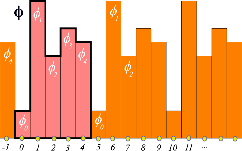
($\mathsf{r}_{1}$) 

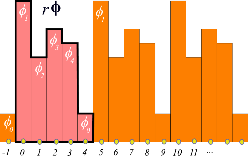
($\mathsf{r}_{2}$) 

($\mathsf{r}_{3}$) 

($\mathsf{r}_{4}$) 

($\mathsf{\sigma}$)  

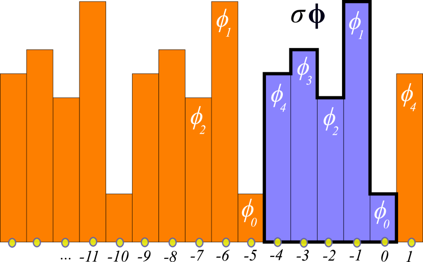
($\mathsf{\sigma}_{1}$) 

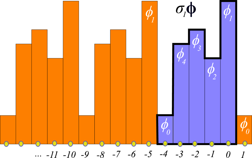
($\mathsf{\sigma}_{2}$) 

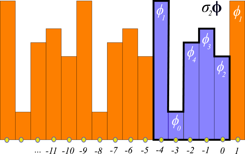
($\mathsf{\sigma}_{3}$) 

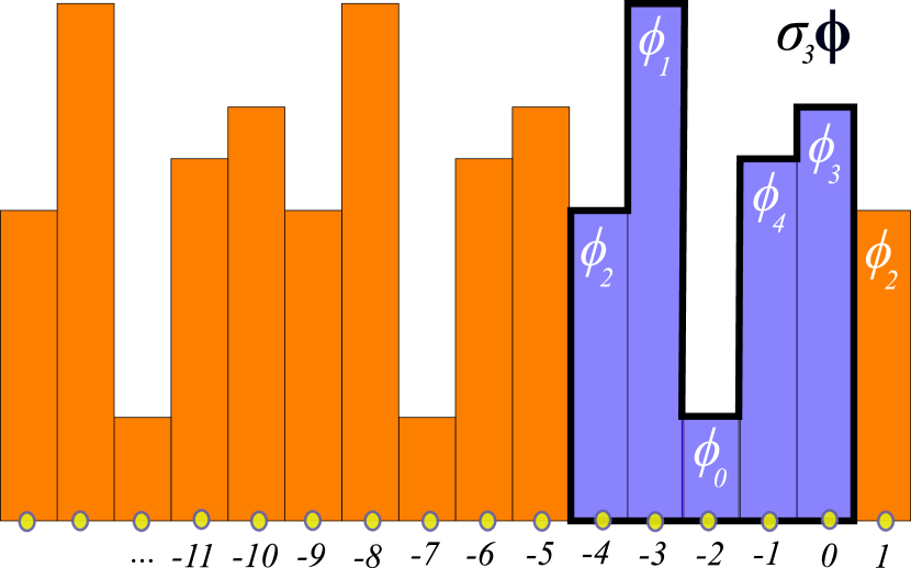
($\mathsf{\sigma}_{4}$) 

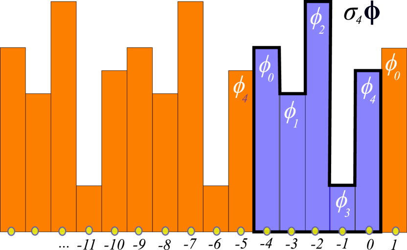
Figure 7: (Color online)    (1) A Bravais cell $\mathbf{a}$ with asymmetric lattice state $\mathsf{\Phi}={\overline{\phi_{0}\phi_{1}\phi_{2}\phi_{3}\phi_{4}}}$, no reflection symmetry, outlined in bold, is invariant under the translation subgroup $H_{5}$. Its $\textrm{C}_{\infty}$ orbit are the ${n}=5$ distinct lattice states (1) to ($\mathsf{r}_{4}$), obtained by all of the $\textrm{C}_{5}$ translations. Its $\textrm{D}_{\infty}$-orbit are $2{n}=10$ distinct lattice states, 5 translations (1) to ($\mathsf{r}_{4}$) and 5 translate-reflections ($\mathsf{\sigma}$) to ($\mathsf{\sigma}_{4}$), obtained by all of the $\textrm{D}_{5}$ actions. See figure 2 (b) for the notation. Continued in figure 8.

Given that $G$ is the symmetry of the system does not mean that $G$ is also the symmetry of its solutions, or what we here call lattice states. They can satisfy all of system’s symmetries, a subgroup of them, or have no symmetry at all. For example, a generic lattice state (8) sketched in figure 6 has no symmetry beyond the identity, so its symmetry group is the trivial subgroup $\{e\}$; any translation $\mathsf{r}_{j}$ or reflection $\mathsf{\sigma}_{k}$ maps it into a different, distinct lattice state, as shown in figure 7. At the other extreme, the constant lattice state $\phi_{j}=\phi$ is invariant under any translation or reflection - its symmetry group is the full $G$, the symmetry of the system. In between, there are lattice states whose symmetry is a subgroup of $G$.

9.6 What are ‘lattice states’? Orbits?

For evolution-in-time, every period-$n$ periodic point is a fixed point of the $n$th iterate of the 1 time-step map. In the lattice formulation, the totality of finite-period lattice states is the set of fixed points of all $H_{\mathbf{a}}$ and $H_{\mathbf{a},k}$ subgroups of $\textrm{D}_{\infty}$.

You can visualize a lattice state invariant under (‘fixed by’) subgroup $H_{\mathbf{a},k}$ as a tiling of the lattice $\mathbb{Z}$ by a lattice state tile of length $n$, symmetric under reflection $\mathsf{\sigma}_{k}$, see figure 9 (b-c).

Definition: Orbit or $G$-orbit of a lattice state $\mathsf{\Phi}$ is the set of all lattice states

$$\mathcal{M}_{\mathsf{\Phi}}=\{g\,\mathsf{\Phi}\mid g\in{G}\}$$ (157)

into which $\mathsf{\Phi}$ is mapped under the action of group $G$. We label the orbit $\mathcal{M}_{\mathsf{\Phi}}$ by any lattice state $\mathsf{\Phi}$ belonging to it.

As an example, the $\textrm{D}_{\infty}$ orbit of the period-5 lattice state is shown in figure 7.

Definition: Symmetry of a solution. We shall refer to the maximal subgroup $G_{\mathsf{\Phi}}\subseteq G$ of actions which permute lattice states within the orbit $\mathcal{M}_{\mathsf{\Phi}}$, but leave the orbit invariant, as the symmetry $G_{\mathsf{\Phi}}$ of the orbit $\mathcal{M}_{\mathsf{\Phi}}$,

$$G_{\mathsf{\Phi}}=\{g\in G_{\mathsf{\Phi}}\mid g\mathcal{M}_{\mathsf{\Phi}}=\mathcal{M}_{\mathsf{\Phi}}\}\,.$$ (158)

An orbit $\mathcal{M}_{\mathsf{\Phi}}$ is $G_{\mathsf{\Phi}}$-symmetric (symmetric, set-wise symmetric, self-dual) if the action of elements of $G_{\mathsf{\Phi}}$ on the set of lattice states $\mathcal{M}_{\mathsf{\Phi}}$ reproduces the orbit.

Definition: Index of orbit $\mathcal{M}_{\mathsf{\Phi}}$ is given by

$$m_{\mathsf{\Phi}}=|G|/|G_{\mathsf{\Phi}}|\,.$$ (159)

(See Wikipedia [182] and Dummit and Foote [73].)

And now, a pleasant surprise, obvious upon an inspection of figures 7 and 9: what happens in the Bravais cell, stays in the Bravais cell. Even though the lattices $\mathcal{L}$, $\mathcal{L}_{\mathbf{a}}$ are infinite, and their symmetries $\textrm{D}_{\infty}$, $H_{\mathbf{a}}$, $H_{\mathbf{a},k}$ are infinite groups, the Bravais lattice states’ orbits are finite, described by the finite group permutations of the infinite lattice curled up into a Bravais cell periodic ${n}$-site ring.

$(\textrm{D}_{3})$

$(\textrm{D}_{4})$

Figure 8: (Color online)    Consider a period-${n}$ Bravais cell tiling of a 1-dimensional lattice $\mathcal{L}$. With $\mathcal{L}$ curled into a ring of ${n}$ lattice sites, actions of the infinite dihedral group $\textrm{D}_{\infty}$ reduce to translational and reflection symmetries of $(\textrm{D}_{3})$ an equilateral triangle, ${n}=3$ lattice sites; $(\textrm{D}_{4})$ a square, ${n}=4$ lattice sites; all group operations that overlie an ${n}$-sided regular polygon onto itself. The ${n}$ translations $\mathsf{r}_{j}$ permute the sites cyclically. The ${n}$ dihedral group $\textrm{D}_{{n}}$ translate-reflect $\mathsf{\sigma}_{k}$ elements (160) reflect the sites across reflection axes, exchanging red and blue sites. For even ${n}$, an even reflection (dashed line reflection axis), here $\mathsf{\sigma}$, leaves a pair of opposite sites fixed (marked yellow), while an odd reflection axis (full line), here $\mathsf{\sigma}_{1}$, bisects the opposite edges, and flips all sites. For odd ${n}$, every reflection half-axis leaves a site fixed (dashed line), and bisects the opposite edge (full line). This periodic ring visualization makes it obvious that any symmetric lattice state is reflection invariant across two points on the lattice, see figure 9.

Indeed, to grasp everything one needs to know about translations $\mathsf{r}_{j}$ (for regular polygons, ‘rotations’), and reflections $\mathsf{\sigma}_{k}$, it suffices to understand the symmetries of an equilateral triangle (dihedral group $\textrm{D}_{3}$) and a square (dihedral group $\textrm{D}_{4}$), depicted in figure 8. It is clear by inspection that an ${n}$-sided regular polygon has ${n}$-fold translational symmetry and ${n}$ reflection symmetry axes. The group of such symmetries is the finite dihedral group

$$\textrm{D}_{{n}}=\{1,\mathsf{\sigma},\mathsf{r},\mathsf{\sigma}_{1},\mathsf{r}_{2},\mathsf{\sigma}_{2},\ \cdots,\mathsf{r}_{{n}-1},\mathsf{\sigma}_{{n}-1}\}$$ (160)

of order $2{n}$. A half of its elements are the ${n}$ cyclic group $\textrm{C}_{n}$ translations $\mathsf{r}_{j}$. The other half are the ${n}$ reflections $\mathsf{\sigma}_{k}$, one for the reflection across each symmetry axis. The group multiplication table is the same as the $\textrm{D}_{\infty}$ (142), but with all subscripts mod ${n}$. As in (147), conjugation by any reflection reverses the direction of translation

$$\mathsf{\sigma}_{i}\mathsf{r}_{j}\mathsf{\sigma}_{-i}=\mathsf{r}_{{n}-j}\,,\qquad 0<j<{n}\,,$$ (161)

so every translation pairs up with the equal counter-translation to form a 2-element class (149).

The distinction between the classes of even and odd reflections (151) is visually self-evident by inspection of figure 8: the symmetry axes either connect opposite lattice sites, or bisect the edges, or both, if ${n}$ is odd (a triangle, for example). One can say that $k$ in the ‘translate-reflection’ (140) operation $\mathsf{\sigma}_{k}$ advances the reflection point by $k$ 1/2 steps, and then reflects across it.

For a polygon with an odd number of lattice sites (a triangle, for example), we see by contemplating the triangle of figure 8, as well as by taking mod ${n}$ of the conjugation relation (150), that all reflections are in the same conjugacy class $\{\mathsf{\sigma}_{j}\}$: there is no splitting into odd and even cases, in contrast to the infinite lattice case (151).

For a polygon with an even number of lattice sites (a square, for example), one must distinguish the ‘long’ axes that connect lattice sites (we label them by even numbers $0,2,\cdots$) from the ‘short’ symmetry axes that bisect opposite edges (labelled by odd numbers $1,3,\cdots$). The corresponding reflections belong to different $\textrm{D}_{{n}}$ (subclasses of (151)),

even reflections $$\quad\{\mathsf{\sigma},\mathsf{\sigma}_{2},\mathsf{\sigma}_{4},\cdots,\mathsf{\sigma}_{{n}/2}\}$$

odd reflections $$\quad\{\mathsf{\sigma}_{1},\mathsf{\sigma}_{3},\cdots,\mathsf{\sigma}_{{n}/2+1}\}\,.$$ (162)

9.7 Symmetries of lattice states

$(a)$     $(o)$
$(ee)$  $(eo)$

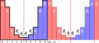
Figure 9: (Color online)    A Bravais lattice state $\mathsf{\Phi}$ has one of the 4 possible symmetries, illustrated by: $(a)$ No reflection symmetry: an $H_{5}$ invariant period-5 lattice state (9.7). For its $G$-orbit, see figure 7. $(o)$ Odd period, reflection-symmetric: an $H_{9,8}$ invariant period-9 lattice state (9.7), reflection symmetric over the lattice sites interval [8-9] midpoint and over the lattice site 4. $(ee)$ Even period, even reflection-symmetric: an $H_{10,0}$ invariant period-10 lattice state (9.7), reflection symmetric over lattice sites 0 and 5. $(eo)$ Even period, odd reflection-symmetric: an $H_{10,9}$ invariant period-10 lattice state (9.7), reflection symmetric over the [4-5] and [9-10] interval midpoints. Horizontal: lattice sites labelled by $t\in\mathbb{Z}$. Vertical: value of field $\phi_{t}$, plotted as a bar centred at lattice site $t$. Time reversed blocks indicated in blue, boundary sites in yellow. Even reflection axes dashed, odd reflections full line.

A Bravais lattice state $\mathsf{\Phi}$ has one of the four symmetries:

asymmetric, no reflection symmetry

$$(a)\quad {\overline{\phi_{0}\phi_{1}\phi_{2}\phi_{3}\cdots\phi_{{n}-1}}}$$

$$\mbox{ index }m_{\mathsf{\Phi}}=2{n}$$

lattice state invariant under the translation group $H_{{n}}$. Its $G$-orbit, generated by all actions of $\textrm{D}_{\infty}$, results in $2{n}$ distinct, $\textrm{D}_{{n}}$ related lattice states. This is illustrated by the $H_{5}$-invariant lattice state $\mathsf{\Phi}$ of figure 7. Its $\textrm{D}_{5}$ orbit are $2{n}=10$ lattice states, 5 translations and 5 translate-reflections.

Next, the reflection-symmetric lattice states. As illustrated in figures 6 and 8, there are two classes (151) of lattice state reflections: even, across a lattice site, and odd, across the mid-point between a pair of adjacent lattice sites. However, as is evident by inspection of figure 8, curling up the lattice $\mathcal{L}$ into a Bravais cell periodic ${n}$-site ring implies that an axis cuts the ring twice, and constrains the possible reflection points to three configurations:

$$\mbox{ odd period }{n}=2m+1$$

$$(o)\quad {\overline{{\framebox{\hskip 1.2pt$\phi_{0}$\hskip 1.2pt}}\phi_{1}\phi_{2}\cdots\phi_{m}|\phi_{m}\cdots\phi_{2}\phi_{1}}}$$

$$\mbox{ index }m_{\mathsf{\Phi}}={n}$$

lattice state invariant under the dihedral group $H_{{n},k}$, illustrated by the $H_{9,8}$ invariant lattice state $\mathsf{\Phi}$ of figure 9 $(o)$.

$$\mbox{ even period }{n}=2m+2\,,\mbox{ even reflection }k$$

$$(ee)\quad {\overline{{\framebox{\hskip 1.2pt$\phi_{0}$\hskip 1.2pt}}\phi_{1}\phi_{2}\cdots\phi_{m}{\framebox{\hskip 1.2pt$\phi_{m+1}$\hskip 1.2pt}}\phi_{m}\cdots\phi_{2}\phi_{1}}}$$

$$\mbox{ index }m_{\mathsf{\Phi}}={n}$$

lattice state invariant under the dihedral group $H_{{n},k}$, $k$ even, illustrated by the $H_{10,0}$ invariant lattice state $\mathsf{\Phi}$ of figure 9 $(ee)$.

$$\mbox{ even period }{n}=2m\,,\mbox{ odd reflection }k$$

$$(eo)\quad {\overline{\phi_{1}\phi_{2}\phi_{3}\cdots\phi_{m}|\phi_{m}\cdots\phi_{2}\phi_{1}|}}$$

$$\mbox{ index }m_{\mathsf{\Phi}}={n}$$

lattice state invariant under the dihedral group $H_{{n},k}$, $k$ odd, illustrated by the $H_{10,9}$ invariant lattice state $\mathsf{\Phi}$ of figure 9 $(eo)$.

The lattice state symmetry $G_{\mathsf{\Phi}}$ (158) of the above $(o)$–$(eo)$ reflection-symmetric lattice states $\mathsf{\Phi}$ is the reflection group $\textrm{D}_{1}=\{1,\mathsf{\sigma}_{k}\}$. This symmetry means two things:

• The $\textrm{D}_{\infty}$ orbits of reflection-symmetric lattice states contain only translations, as any reflection amounts to a cyclic group $\textrm{C}_{{n}}$ translation. (Reflect a lattice state in figure 9 (b-d) over any lattice site or mid-interval: the result is its translation.)

• The prime lattice state is a ‘half’ of the Bravais cell, the length ${m}$ orbit,

  $$\tilde{\mathsf{\Phi}}=(\phi_{1}\phi_{2}\phi_{3}\cdots\phi_{m})\,,$$ (167)

  give or take some boundary sites.

To develop intuition about how one reconstructs the period-${n}$ orbit from this length-$m$ block it is helpful to have a look at explicit matrix representation of the dihedral group $\textrm{D}_{{n}}$ actions.

9.8 Permutation representation

A lattice state $\mathsf{\Phi}$ over a Bravais cell $\mathbf{a}$ can be assembled into an ${n}$-dimensional vector whose components are lattice site fields

$${\mathsf{\Phi}}{}^{\top}=(\phi_{0},\phi_{1},\phi_{2},\phi_{3},\cdots,\phi_{{n}-1})\,.$$ (168)

Matrices that reshuffle the components of such vectors form the permutation representation of a finite group $G$. They give us a different perspective on the above three kinds of symmetric solutions.

The permutation representation of 1-step lattice translation $\mathsf{r}$ acts on a Bravais lattice state by the off-diagonal $[{n}\!\times\!{n}]$ matrix (31). This is a cyclic $\textrm{C}_{{n}}$ permutation that translates the lattice state $\mathsf{\Phi}$ ”forward-in-time” by one site,

$${(\mathsf{r}\mathsf{\Phi})}{}^{\top}=(\phi_{1},\phi_{2},\cdots,\phi_{{n}-1},\phi_{0})\,.$$

A permutation representation of a $\textrm{D}_{{n}}$ translate-reflect operation is essentially an anti-diagonal matrix that reverses the order of site fields, up to a cyclic permutation

$${(\mathsf{\sigma}_{k}\mathsf{\Phi})}{}^{\top}=(\phi_{{n}-1},\cdots,\phi_{2},\phi_{1},\phi_{0})\,.$$

Even periods: The shortest even period symmetric lattice state is the period-2 lattice state ${\mathsf{\Phi}_{p}}{}^{\top}=(\phi_{0},\phi_{1})$ such as the temporal cat (130). For example, for temporal Hénon (53) there is only one period-2 prime orbit, consisting of lattice state

$$\mathsf{\Phi}_{p}=\frac{1}{a}\left(\begin{array}[]{c}-1-\sqrt{a-3}\cr-1+\sqrt{a-3}\end{array}\right)\,,$$ (169)

and its translation $\mathsf{r}\mathsf{\Phi}_{p}$. Its symmetry, ${\mathsf{\Phi}_{p}}{}^{\top}=({\framebox{\hskip 1.2pt$\phi_{0}$\hskip 1.2pt}}\,{\framebox{\hskip 1.2pt$\phi_{1}$\hskip 1.2pt}})$ is of $(ee)$ type (9.7), indicated as yellow lattice sites fields in figure 9 $(ee)$. Its orbit Jacobian matrix is of the nonlinear field theory form (74)

$${\mathcal{J}}=\left(\begin{array}[]{cc}s_{0}&-2\\ -2&s_{1}\end{array}\right)\,.$$ (170)

This lattice state is ‘all boundary points’, too short to illustrate a symmetry reduction to a $D_{{n}}$ prime orbit. Still, as we show in figure 12 (b), its relation to the block circulant structure of repeated-tile orbit Jacobian matrix (80) and its contribution to $\phi^{3}$ field theory spectrum is instructive.

Odd periods: In odd dimensions, the ${n}$ translate-reflect matrices of $\textrm{D}_{{n}}$ are related by translations (150). For example, for a period-3 lattice state without symmetry ${\mathsf{\Phi}}{}^{\top}=(\phi_{0},\phi_{1},\phi_{2})\,,$ they are

$$\mathsf{\sigma}=\left(\begin{array}[]{ccc}1&0&0\\ 0&0&1\\ 0&1&0\end{array}\right)\,,\quad{\mathsf{\sigma}_{1}}=\left(\begin{array}[]{ccc}0&1&0\\ 1&0&0\\ 0&0&1\end{array}\right)\,,\quad\mathsf{\sigma}_{2}=\left(\begin{array}[]{ccc}0&0&1\\ 0&1&0\\ 1&0&0\end{array}\right)\,.$$

In agreement with (9.7), figure 8 and figure 9 $(o)$, these reflections keep one lattice site fixed (for each permutation matrix $\mathsf{\sigma}_{k}$ there is only one ‘1’ on the diagonal), swap the rest.

To get some insight into the length-${m}$ prime lattice state $\tilde{\mathsf{\Phi}}$ (167), consider next a period-5 reflection symmetric lattice states that tile the infinite lattice $\mathcal{L}$ with a reflection-fixed  $\phi_{0}$ , and a length-2 block $\tilde{\mathsf{\Phi}}=(\phi_{1},\phi_{2})$,

$${\mathsf{\Phi}}{}^{\top}=({\framebox{\hskip 1.2pt$\phi_{0}$\hskip 1.2pt}}\phi_{1}\phi_{2}|\phi_{2}\phi_{1})\,.$$ (171)

Actions of $\textrm{D}_{5}$ permutation representation illustrates that the fixed lattice states $\mathsf{\Phi}$ of $\mathsf{\sigma}_{k}$ are related by cyclic translations:

$$\mathsf{\sigma}\mathsf{\Phi} = \left(\begin{array}[]{ccccc}1&0&0&0&0\\ 0&0&0&0&1\\ 0&0&0&1&0\\ 0&0&1&0&0\\ 0&1&0&0&0\end{array}\right)\left(\begin{array}[]{c}{\framebox{\hskip 1.2pt$\phi_{0}$\hskip 1.2pt}}\cr\phi_{1}\cr\phi_{2}\cr\phi_{2}\cr\phi_{1}\cr\end{array}\right)=\left(\begin{array}[]{c}{\framebox{\hskip 1.2pt$\phi_{0}$\hskip 1.2pt}}\cr\phi_{1}\cr\phi_{2}\cr\phi_{2}\cr\phi_{1}\cr\end{array}\right)$$ (187)

$$\mathsf{\sigma}_{4}(\mathsf{r}_{-2}\mathsf{\Phi}) = \left(\begin{array}[]{ccccc}0&0&0&0&1\\ 0&0&0&1&0\\ 0&0&1&0&0\\ 0&1&0&0&0\\ 1&0&0&0&0\end{array}\right)\left(\begin{array}[]{c}\phi_{2}\cr\phi_{1}\cr{\framebox{\hskip 1.2pt$\phi_{0}$\hskip 1.2pt}}\cr\phi_{1}\cr\phi_{2}\cr\end{array}\right)=\left(\begin{array}[]{c}\phi_{2}\cr\phi_{1}\cr{\framebox{\hskip 1.2pt$\phi_{0}$\hskip 1.2pt}}\cr\phi_{1}\cr\phi_{2}\cr\end{array}\right)\,.$$ (203)

What is the orbit stability of such lattice state? The symmetry conditions are the Bravais lattice state 5-periodicity mod 5, and the even reflection across  $\phi_{0}$ :

$$\phi_{i}=\phi_{i+5}\,,\quad\phi_{-i}=\phi_{i}\,.$$ (204)

A lattice state satisfies the Euler–Lagrange equation (51)

$$-\phi_{t-1}+2\phi_{t}-\phi_{t+1}+V^{\prime}(\phi_{t})=0\,,$$ (205)

on the period-5 Bravais cell,

$$-\phi_{1}+2\phi_{0}-\phi_{1}+V^{\prime}(\phi_{0}) = 0$$

$$-\phi_{0}+2\phi_{1}-\phi_{2}+V^{\prime}(\phi_{1}) = 0$$

$$-\phi_{1}+2\phi_{2}-\phi_{2}+V^{\prime}(\phi_{2}) = 0$$

$$-\phi_{1}+2\phi_{2}-\phi_{2}+V^{\prime}(\phi_{2}) = 0$$

$$-\phi_{0}+2\phi_{1}-\phi_{2}+V^{\prime}(\phi_{1}) = 0\,,$$ (206)

where we have used (204). The result are symmetry reduced equations, modified by the two reflection bc’s,

$$-2\phi_{1}+2\phi_{0}+V^{\prime}(\phi_{0}) = 0$$

$$-\phi_{0}+2\phi_{1}-\phi_{2}+V^{\prime}(\phi_{1}) = 0$$

$$-\phi_{1}+\phi_{2}+V^{\prime}(\phi_{2}) = 0\,,$$ (207)

with an asymmetric 3-dimensional orbit Jacobian matrix (74)

$${\mathcal{J}}_{o} = \left(\begin{array}[]{ccc}{s}_{0}&-2&0\\ -1&{s}_{1}&-1\\ 0&-1&{s}_{2}-1\end{array}\right)\,.$$ (211)

So, for a reflection-symmetric lattice state of odd period, one has to impose the even  $\phi_{0}$  and odd $|$ reflection bc’s in order to define the orbit Jacobian matrix for the prime orbit $\tilde{\mathsf{\Phi}}$ (167).

The form of orbit Jacobian matrices for all bc’s of section 9.7, specialized to temporal cat but easily generalized to general nonlinear field theories, is given in C.

Why bother?

ChaosBook.org [53] bemoans more than 20 times that in it the time-reversal symmetric orbits are not accounted for (here that is accomplished in section 11). But for long periods, almost all lattice states are of asymmetric type (9.7). Why do we obsess about symmetric lattice states so much? How important are they?

The reason is that periodic orbit expansions are dominated by short orbits, with the longer ones only providing exponentially small corrections. But almost all short-period lattice states are symmetric; for example, for the $\phi^{3}$ field theory, the first two asymmetric lattice states of are of period 6.

10 Reciprocal lattice

If the orbit Jacobian matrix is invariant under time translation, its eigenvalue spectrum and Hill determinant can be efficiently computed using tools of crystallography, such as the discrete Fourier transform, a discretization approach that goes all the way back to Hill’s 1886 paper [102].

Think of a solution of a discrete time dynamical system as a 1-dimensional lattice state with the field on each site labeled by integer time. A time period-${n}$ lattice state lives on a discrete 1-torus (a ring or chain or necklace) of period-${n}$, and if system’s law is time-invariant, its orbit, the set of lattice states related to it by cyclic translations, are physically equivalent (figure 7). The symmetry is the cyclic group $\textrm{C}_{n}$, and one only needs to count and distinguish $\textrm{C}_{n}$ orbits, compute only one lattice state per each orbit.

The smart way to do this is by a discrete Fourier transform. Were the lattice $d$-dimensional (4), defined by Bravais cell vectors $\{\mathbf{a}\}$, a crystallographer would immediately move to the reciprocal lattice, $\tilde{\mathcal{L}}_{\mathbf{b}}=\{k\mathbf{b}\,|\,k\in\mathbb{Z}\}\,,$ with reciprocal lattice basis vectors $\{\mathbf{b}\}$ satisfing $\mathbf{b}\!\cdot\!\mathbf{a}=2\pi\,.$ On the reciprocal lattice translations are quotiented out, and calculations are restricted to a finite Brilluoin zone (Bloch’s theorem of solid state physics). Here we work on a 1-dimensional lattice with unit lattice spacing 1, so the reciprocal lattice spacing is $2\pi/1=2\pi$, with the (first) Brillouin zone from $k=-\pi$ to $k=\pi$ (we give an example in figure 12).

The cyclic group $\textrm{C}_{n}$ elements are generated by the $[{n}\!\times\!{n}]$ shift matrix (31) which translates a lattice state (9) forward-in-time by one site, ${(\mathsf{r}\mathsf{\Phi})}{}^{\top}=(\phi_{1},\phi_{2},\cdots,\phi_{{n}-1},\phi_{0})$. After ${n}$ shifts, the lattice state returns to the initial state, yielding the characteristic equation for the matrix $\mathsf{r}$

$$\mathsf{r}^{n}-{\ \hbox{{\rm 1}\kern-6.19995pt\hbox{\rm 1}}}=0\,,$$ (212)

whose eigenvalues are ${n}$th roots of unity, with the ${n}$ complex eigenvectors also built from roots of unity

$$\{\lambda_{k}\} = \{1,\omega,\omega^{2},\cdots,\omega^{{n}-1}\}\,,\qquad\qquad\quad\omega=\rme^{2\pi\mathrm{i}/{n}}$$

$$\tilde{e}_{k} = \frac{1}{\sqrt{{n}}}(1,\omega^{k},\omega^{2k},\ldots,\omega^{k({n}-1)})\,,\qquad k=0,1,\ldots,{n}-1\,.$$ (213)

10.1 Reciprocal lattice states

In the $\{\tilde{e}_{k}\}$ Fourier basis, a real ${n}$-dimensional lattice state vector $\mathsf{\Phi}$ is mapped onto a ${n}$-dimensional complex reciprocal lattice vector

$$\tilde{\mathsf{\Phi}}=(\tilde{\phi}_{0},\tilde{\phi}_{1},\tilde{\phi}_{2},\dots,\tilde{\phi}_{{n}-1})\,,$$ (214)

with the $k$th Fourier mode of magnitude $|\tilde{\phi}_{k}|$ and phase $e^{i\theta_{k}}$.

On the reciprocal lattice, the shift matrix is diagonal, $\mathsf{r}_{jk}=\omega^{k}\,\delta_{jk}$, and the ‘time’ dynamics is breathtakingly simple: no matter what the dynamical system is, in one time step $\mathsf{\Phi}\to\mathsf{r}\mathsf{\Phi}$, the $k$th Fourier mode phase is incremented by a fraction of the circle,

$$(\tilde{\phi}_{0},\tilde{\phi}_{1},\tilde{\phi}_{2},\dots,\tilde{\phi}_{{n}-1}) \to (\tilde{\phi}_{0},\omega\tilde{\phi}_{1},\omega^{2}\tilde{\phi}_{2},\dots,\omega^{{n}-1}\tilde{\phi}_{{n}-1})$$

$$e^{\mathrm{i}\theta_{k}} \to e^{\mathrm{i}(\theta_{k}+2\pi{k}/{n})}\,,$$ (215)

so reciprocal lattice states literally run in circles; for non-zero $k$ and $|\tilde{\phi}_{k}|$, all reciprocal lattice states lie on vertices of regular complex plane ${n}$-gons, inscribed in circles of radius $|\tilde{\phi}_{k}|$, one circle for each orbit.

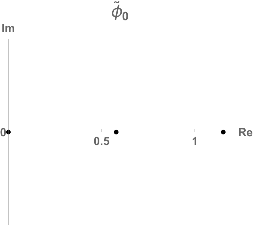
(a)

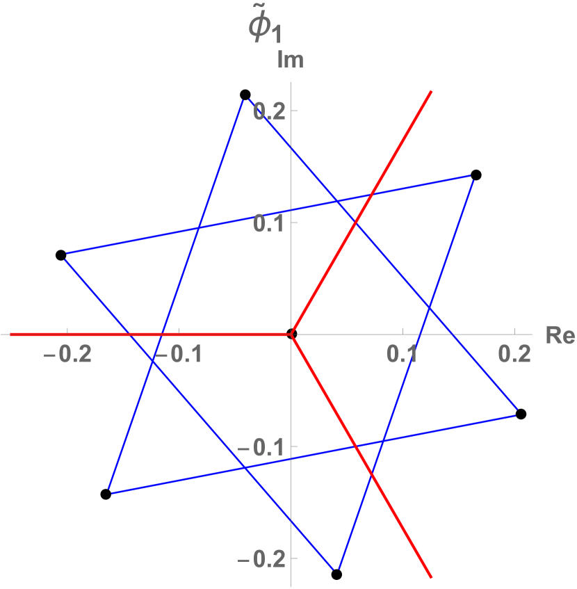
(b)

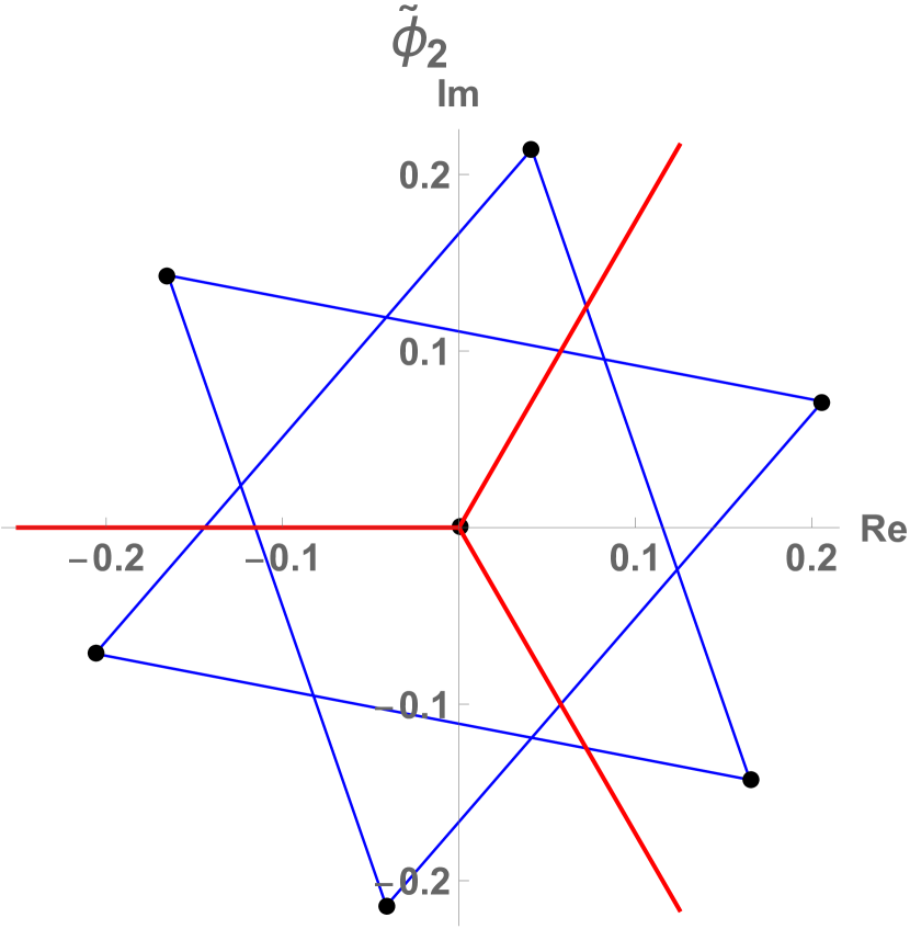
(c)

Figure 10: (Color online)    The reciprocal lattice $(\tilde{\phi}_{0},\tilde{\phi}_{1},\tilde{\phi}_{2})$ Fourier components of the 7 $\textrm{C}_{3}$-equivariant period-3 lattice states, $s=2$ temporal Bernoulli system (29). In $\tilde{\phi}_{1}$ and $\tilde{\phi}_{2}$ complex planes, reciprocal lattice states lie on vertices of the 2 equilateral triangles, one for each $\textrm{C}_{3}$ orbit, while the component at the origin is the fixed point $\mathsf{\Phi}=(0,0,0)$. The $\textrm{C}_{3}$ fundamental domain indicated by red border lines contains non-zero reciprocal lattice states whose phases lie in the $[-2\pi/6,2\pi/6)$ wedge, one reciprocal lattice state for each distinct $\textrm{C}_{3}$ orbit.

As a concrete example, consider the period-3 lattice states of the temporal Bernoulli (29) for stretching parameter $s=2$. It is a linear problem and all lattice states are easily computed by hand, one for each symbol block $\mathsf{M}$. There is always the fixed point lattice state $(0,0,0)$ at the origin, and the remaining lattice states belong to $M_{3}=2$ period-3 orbits, where $M_{n}$ is the number of orbits of period ${n}$. Discrete Fourier transform maps these 2 orbits into reciprocal lattice $(\tilde{\phi}_{0},\tilde{\phi}_{1},\tilde{\phi}_{2})$ triangles, see figure 10. The time-step $\mathsf{r}$ acts on the $\tilde{\phi}_{1}$, $\tilde{\phi}_{2}$ components by complex 1/3-circle phase rotations $\exp(2\pi\mathrm{i}/3)$ and $\exp(4\pi\mathrm{i}/3)$, respectively: reciprocal lattice states connected by blue lines in figure 10 lie on a circle and belong to the same orbit. In this example the two orbits happen to lie on the same circle, as they are related by the internal $\textrm{D}_{1}:\phi_{i}\to 1-\phi_{i}$ symmetry of the Bernoulli system, see section 9.1.

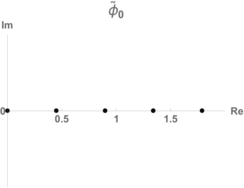
(a)

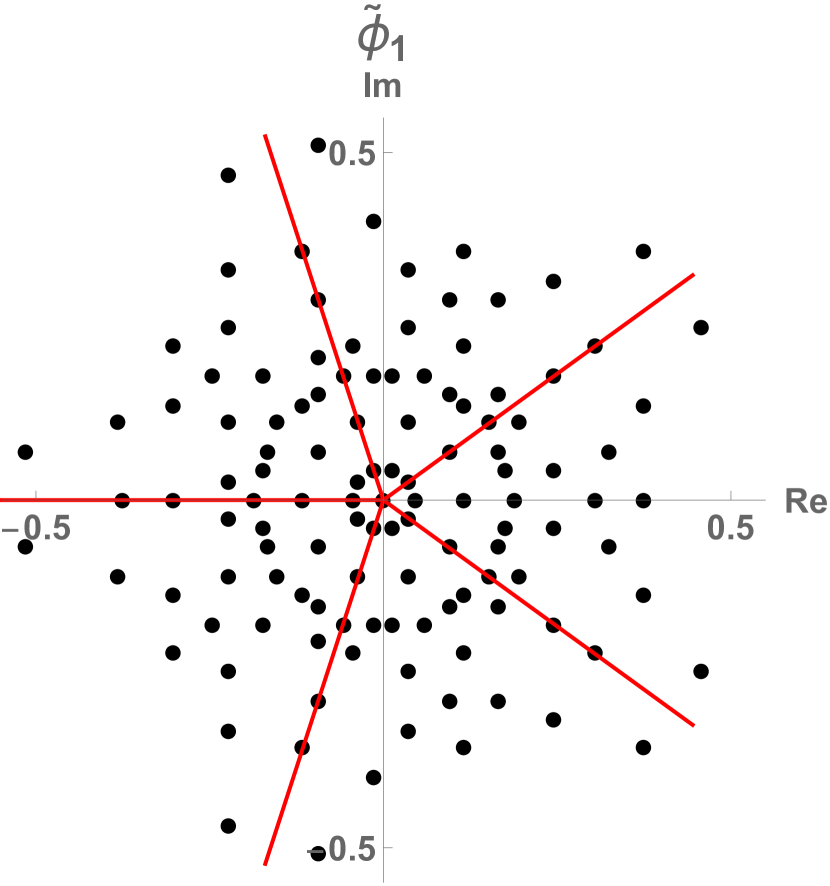
(b)

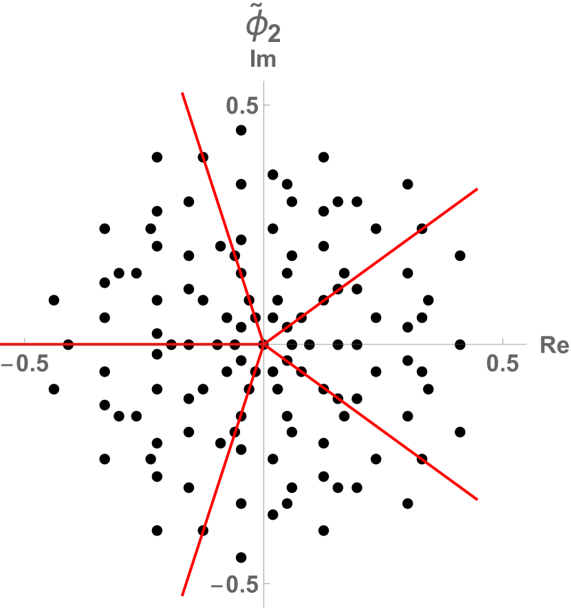
(c)

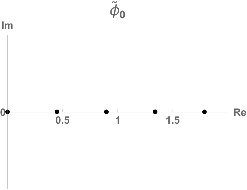
(d)

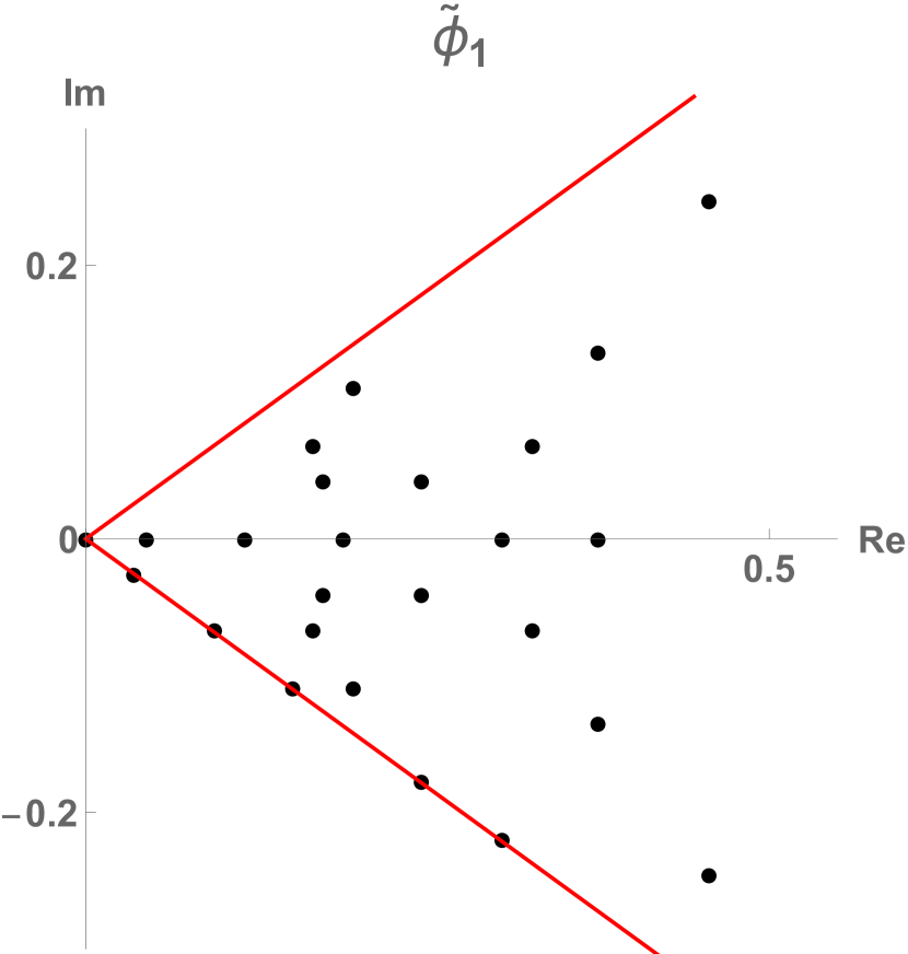
(e)

(f)

Figure 11: (Color online)    The 121 period-5 reciprocal lattice states of the $s=3$ temporal cat (43). (a,b,c) The reciprocal lattice $\tilde{\phi}_{0},\tilde{\phi}_{1},\tilde{\phi}_{2}$ complex planes. The state at the origin is the fixed point $(0,0,0,0,0)$. As in figure 10, all non-zero reciprocal lattice states lie on vertices of regular pentagons (not drawn here) that form orbits under $\textrm{C}_{5}$ cyclic permutations. (d,e,f) The $\textrm{C}_{5}$ fundamental domain contains $M_{5}=24$ non-zero reciprocal lattice states whose phases lie in the $[-2\pi/10,2\pi/10)$ wedge, one reciprocal lattice state for each distinct $\textrm{C}_{5}$ orbit.

10.1.1 $\textrm{C}_{{n}}$ fundamental domain.

Divide each $k>0$ complex $\tilde{\phi}_{k}$ plane of a period-${n}$ reciprocal lattice state into ${n}$ equal wedges, and call one of them the ‘fundamental domain’, for example the wedge bordered by $[-\pi/{n},\pi/{n})$. Under ${n}$ discrete rotations the fundamental domain completely tiles the complex plane. We exclude the fixed point lattice state $\tilde{\phi}_{k}=0$ at the origin from the domain, as it belongs to a time invariant subspace.

As is clear by inspection of figure 10, every $k$th complex plane regular ${n}$-gon has precisely one vertex, i.e., a single reciprocal lattice state per each orbit, in the interior of the fundamental domain, or on its border. For the period-3 reciprocal lattice states shown in figure 10, there are 2 points in both $k=2$ and $k=3$ complex plane fundamental domain, one lattice state for each period-3 orbit.

Consider next the 121 period-5 reciprocal lattice states of the $s=3$ temporal cat (43), figure 11 (a,b,c). Excluding the fixed point $\tilde{\phi}_{k}=0$ lattice state at the origin, there are $M_{5}=24$ reciprocal lattice states in the figure 11 (d,e,f) fundamental domain, each representing ${n}=5$ lattice states in its orbit, so the total number of lattice states is $N_{5}=1+5\,M_{5}=1+5\times 24=121$, in agreement with table 2.

The set of period-5 reciprocal lattice states of Figure 11 clearly exhibits symmetries beyond the cyclic $\textrm{C}_{5}$, in particular under reflections across the axes drawn in red. It also turns out that for the temporal cat the $\tilde{\phi}_{1}$ complex plane looks the same as the $\tilde{\phi}_{4}$ complex plane, and $\tilde{\phi}_{2}$ the same as $\tilde{\phi}_{3}$, so we do not plot them here. Furthermore, for period ${n}$ not a prime number, some $|\tilde{\phi}_{k}|$ might vanish. We shall return to these symmetries in section 10.3.

10.2 Spectra of orbit Jacobian matrices

As the period of a lattice state gets longer, the orbit Jacobian matrix becomes larger and the Hill determinant becomes harder to compute. For a period-$n$ lattice state, ${\mathcal{J}}$ is a matrix with $n$ eigenvalues and eigenvectors. What are they? What are the magnitudes of these eigenvalues?

10.2.1 Spectra of translationally invariant orbit Jacobian matrices.

Orbit Jacobian matrices of the temporal Bernoulli (71) and temporal cat (71) consist of only identity matrix and cyclic shift matrix, whose eigenvectors are discrete Fourier basis (213), so they are diagonalized by discrete Fourier transform. In the space of reciprocal lattice states, orbit Jacobian matrices (71) and (71) are diagonal, each diagonal element an eigenvalues of orbit Jacobian matrices, for the temporal Bernoulli

$$({s}{\ \hbox{{\rm 1}\kern-6.19995pt\hbox{\rm 1}}}-{\mathsf{r}})\,\tilde{e}_{k}=({s}-\omega^{k})\,\tilde{e}_{k}\,,$$ (216)

and for the temporal cat

$$(-\mathsf{r}+{s}\,{\ \hbox{{\rm 1}\kern-6.19995pt\hbox{\rm 1}}}-\mathsf{r}^{-1})\,\tilde{e}_{k}=\left[{s}-2\cos\left(\frac{2\pi k}{{n}}\right)\right]\,\tilde{e}_{k}\,.$$ (217)

Determinants are products of eigenvalues, so the temporal Bernoulli Hill determinant for any period-$n$ lattice state is

$$\mbox{\rm Det}\,({s}{\ \hbox{{\rm 1}\kern-6.19995pt\hbox{\rm 1}}}-{\mathsf{r}})=\prod_{k=0}^{{n}-1}({s}-\omega^{k})=s^{{n}}-1\,,$$ (218)

in agreement with the time-evolution count (27) and Hill’s formula calculation (103). The temporal cat Hill determinant is

$$\mbox{\rm Det}\,(-\mathsf{r}+{s}\,{\ \hbox{{\rm 1}\kern-6.19995pt\hbox{\rm 1}}}-\mathsf{r}^{-1})=\prod_{k=0}^{{n}-1}\left[{s}-2\cos\left(\frac{2\pi k}{{n}}\right)\right]=2\,T_{{n}}\left({s}/{2}\right)-2\,,$$ (219)

confirming the $2$nd-order inhomogeneous difference equation calculation (133).

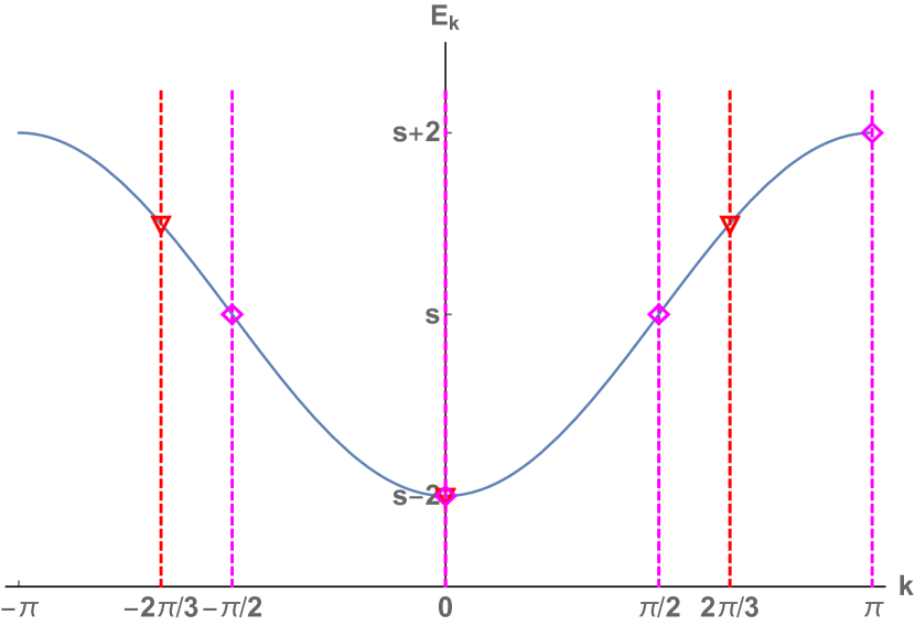
(a)

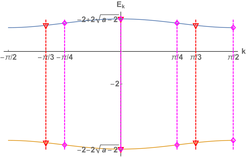
(b)

Figure 12: (Color online)    Infinite lattice orbit Jacobian matrix first Brillouin zone spectra, as functions of the reciprocal lattice wavenumber $k$. For time-reversal invariant systems the spectra are $k\to-k$ symmetric. (a) The temporal cat $E(k)$ spectrum (222). Any period-$n$ lattice state spectrum consists of $n$ discrete points embedded into $E(k)$, for example period-3 (red triangles) and period-4 (magenta diamonds) lattice states eigenvalues (225). There are only 4 reciprocal lattice states, as $k=\pi$ and $k=-\pi$ differ by a reciprocal lattice translation, and are counted only once. (b) The temporal Hénon $E(k)_{\pm}$ spectrum (228) of the infinite lattice tiled by athe period-2 lattice state, together with the eigenvalues of repeats (229) for 1st repeat, 3rd repeat (red triangles) and 4th repeat (magenta diamonds).

The orbit Jacobian matrix (68) of a period-$n$ lattice state is an $[{n}\!\times\!{n}]$ matrix. For an infinite lattice state, the orbit Jacobian matrix is an infinite-dimensional linear operator. For example, the temporal cat infinite-dimensional orbit Jacobian matrix has the form (71), where the time translation operator $\mathsf{r}$ implements the translation on the infinite lattice. The orbit Jacobian matrix commutes with the time translation operator, so its symmetry is the infinite cyclic group of integer lattice translations (139). By Bloch’s theorem an eigenstate of the linear operator ${\mathcal{J}}$ is of form

$$\psi_{k}(t)=e^{\mathrm{i}kt}u_{k}(t)\,,$$ (220)

where $u_{k}(t)$ is a period-1 periodic function. The orbit Jacobian matrix only acts on the field over the integer lattice, on which the periodic function $u_{k}(t)$ is a constant. The eigenstates

$$(\psi_{k})_{t}=\psi_{k}(t)=e^{\mathrm{i}kt}\,,\quad t\in\mathbb{Z}\,,$$ (221)

are plane waves on the lattice. The wavenumber $k$ of the eigenstate $\psi_{k}$ can always be restricted to the first Brillouin zone, $k\in[-\pi,\pi)$. Action of the orbit Jacobian matrix (71) on the wavenumber $k$ eigenstate (221) yields eigenvalue

$$E(k)\psi_{k}={\mathcal{J}}\psi_{k}=(s-2\cos k)\psi_{k}\,,$$ (222)

plotted in the first Brillouin zone in figure 12 (a). The infinite lattice spectrum contains all eigenvalues of orbit Jacobian matrices for any period-$n$ lattice state. The period-$n$ boundary condition is

$$\psi_{k}(t+{n})=\psi_{k}(t)\,,$$ (223)

hence the wavenumber $k$ is restricted to the $n$ first Brillouin zone values $k=2\pi l/{n}$, where $l$ is an integer, with eigenvalues

$$E_{k}\psi_{k}={\mathcal{J}}\psi_{k}=(s-2\cos k)\psi_{k}\,,\qquad k=\frac{2\pi l}{{n}}\,,\quad l\in\mathbb{Z}\,,$$ (224)

in agreement with (217). For example, for the period-1, period-3 and the period-4 lattice states the wavenumbers and corresponding eigenvalues are, respectively

$$(k_{0}) = (0)\,,\quad(\lambda_{0})=(s-2)$$

$$(k_{-1},k_{0},k_{1}) = (-\frac{2\pi}{3},0,\frac{2\pi}{3})$$

$$(\lambda_{-1},\lambda_{0},\lambda_{1}) = (s+1,s-2,s+1)$$

$$(k_{-1},k_{0},k_{1},k_{2}) = (-\frac{\pi}{4},0,\frac{\pi}{4},\frac{\pi}{2})$$

$$(\lambda_{-1},\lambda_{0},\lambda_{1},\lambda_{2}) = (s,s-2,s,s+2)\,,$$ (225)

plotted in figure 12 (a).

In summary: for a field theory with translationally invariant, uniform stretching parameter $s$ orbit Jacobian matrices, eigenvalues of any lattice state are embedded in a single first Brillouin zone spectrum $E(k)$, the blue curve in figure 12 (a). As long as the Klein-Gordon mass $\mu^{2}=s-2>0$ is positive, all lattice states are unstable, and the field theory is chaotic.

10.2.2 Spectra of nonlinear field theories.

For a nonlinear field theory, the orbit Jacobian matrix (74) of a general prime lattice state is not translationally invariant. The orbit Jacobian matrix of a repeat of a period-$n$ prime lattice state, however, is a tri-diagonal block circulant matrix (80), which commutes with the translation operator $\mathsf{r}^{{n}}$. For an infinite lattice state tiled by repeats of a period-$n$ prime lattice state $\mathsf{\Phi}_{p}$ (see figure 7 (1) for a sketch), the infinite-dimensional orbit Jacobian matrix is invariant under $\mathsf{r}^{n}$ translation subgroup (144). Now we can apply Bloch’s theorem to Bravais lattice ${n}\mathbb{Z}$, with an eigenstate of the orbit Jacobian matrix a plane wave times a periodic function (220), where $u_{k}(t)$ is a periodic function with period $n$. The wavenumber $k$ is restricted in the first Brillouin zone of the Bravais lattice ${n}\mathbb{Z}$, $k\in[-\pi/{n},\pi/{n})$. Using the Bloch’s theorem (220) we can find the eigenvalue spectrum of the orbit Jacobian matrix of a prime lattice state $\mathsf{\Phi}_{p}$’s repeats.

This infinite lattice spectrum contains eigenvalues of orbit Jacobian matrix of the infinite repeat of the prime lattice state $\mathsf{\Phi}_{p}$. To find eigenvalues of the orbit Jacobian matrix of the ${m}$th repeat of $\mathsf{\Phi}_{p}$ (80), we need to only use the period-$({m}{n})$ eigenstates, which satisfy:

$$\psi_{k}(t+{m}{n})=\psi_{k}(t)\,.$$ (226)

The wavenumber $k$ must exist on the reciprocal lattice of the Bravais lattice spanned by $({m}{n})$, i.e., $k=2\pi l/({m}{n})$, where $l$ is an integer.

As an example, consider the temporal Hénon period-2 lattice state $\mathsf{\Phi}_{p}$ (169), with a 2-dimensional repeating block (170) orbit Jacobian matrix. The orbit Jacobian matrix of an infinite lattice state tiled by repeats of $\mathsf{\Phi}_{p}$ is the infinite-dimensional linear operator

$${\mathcal{J}}=\left(\begin{array}[]{ccccc}\ddots&\ddots&&&\\ \ddots&s_{1}&-1&&\\ &-1&s_{0}&-1&\\ &&-1&s_{1}&\ddots\\ &&&\ddots&\ddots\\ \end{array}\right)\,,\quad\left(\begin{array}[]{c}s_{0}\cr s_{1}\end{array}\right)=\left(\begin{array}[]{c}-2-2\sqrt{a-3}\cr-2+2\sqrt{a-3}\end{array}\right)$$ (227)

whose eigenstates are plane waves of form (220), where $u_{k}(t)$ is periodic with period 2. Now there are two families of ${\mathcal{J}}$ eigenvalues:

$$E(k)^{\pm}\psi_{k}={\mathcal{J}}\psi_{k}=-2(1\pm\sqrt{a-3+\cos^{2}k})\,\psi_{k}\,,$$ (228)

plotted in the first Brillouin zone $k\in[-\pi/2,\pi/2)$ in figure 12 (b).

The eigenvalues of the orbit Jacobian matrices of the $m$th repeat of $\mathsf{\Phi}_{p}$ are $2m$ points in the spectrum (228), at $k=2\pi l/(2m)$, where $l$ is an integer. For example, for the single repeat (see orbit Jacobian matrix (170)), the 3rd repeat and the 4th repeat the wavenumbers and corresponding eigenvalues are, respectively

$$(k_{0}) = (0)\,,\quad(\lambda^{\pm}_{0})=(-2\pm 2\sqrt{a-2})$$

$$(k_{-1},k_{0},k_{1}) = (-\frac{\pi}{3},0,\frac{\pi}{3})$$

$$(\lambda^{\pm}_{-1},\lambda^{\pm}_{0},\lambda^{\pm}_{1}) = (-2\pm\sqrt{4a-11},-2\pm 2\sqrt{a-2},-2\pm\sqrt{4a-11})$$

$$(k_{-1},k_{0},k_{1},k_{2}) = (-\frac{\pi}{4},0,\frac{\pi}{4},\pi/2)$$

$$(\lambda^{\pm}_{-1},\lambda^{\pm}_{0},\lambda^{\pm}_{1},\lambda^{\pm}_{2}) = (-2\pm\sqrt{4a-10},-2\pm 2\sqrt{a-2},$$ (229)

$$-2\pm\sqrt{4a-10},-2\pm 2\sqrt{a-3})\,,$$

plotted in figure 12 (b).

In summary: for a nonlinear field theory, each period-$n$ prime lattice state $\mathsf{\Phi}_{p}$ has up to $n$ distinct eigenvalues $\{\lambda^{(j)}\}$, each with its own infinite lattice spectrum family $E(k)^{(j)}$ into which eigenvalues of all repeats of $\mathsf{\Phi}_{p}$ are embedded.

10.3 Reciprocal lattice visualization of system’s symmetries

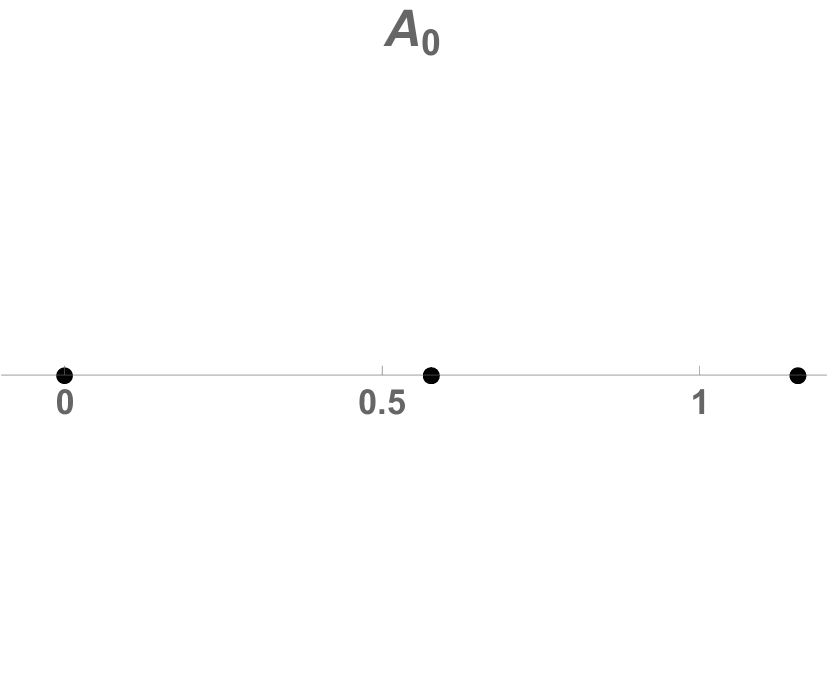
(a)

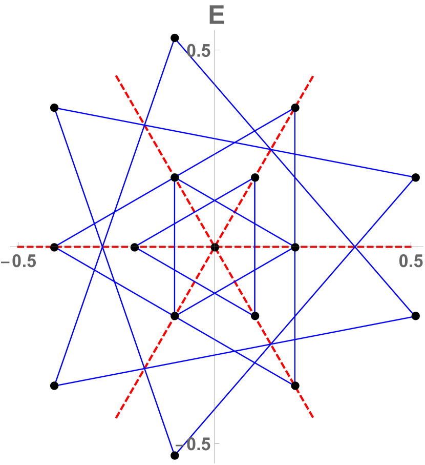
(b)

Figure 13: (Color online)    Period-3 reciprocal lattice states of the $s=3$ temporal cat, plotted in the $\textrm{D}_{3}$ permutation representation irreducible subspaces $A_{0}+E$. (a) $A_{0}$ representation is the one-dimensional, time invariant ‘center of mass’ of the orbit. (b) In contrast to the $\textrm{C}_{{n}}$ complex irreps of figure 10, the 2-dimensional irreps $E_{k}$ of $\textrm{D}_{{n}}$ are real. In the $E_{k}$ planes reciprocal lattice states related by cyclic permutations and reflections lie on vertices of ${n}$-gons or pairs of ${n}$-gons. For $\textrm{D}_{3}$ they lie on triangles, with cyclic sets connected by blue lines. The 2 big triangles are a single $\textrm{D}_{3}$ 6-lattice states orbit, what for $\textrm{C}_{3}$ is a pair of 3-lattice states orbits, with time reversal symmetry ignored. The remaining 3 smaller triangles are 3 time-reversal symmetric orbits. The small pair in the center would be two distinct radius $\textrm{D}_{3}$ orbits, where they not related by the internal symmetry $\textrm{D}_{1}:\phi_{i}\to 1-\phi_{i}$ specific to the spatiotemporal cat (see section 9.1). The state in the center is the fixed point $\phi_{0}=0$. Red dashed lines are the reflection axes of the $\textrm{D}_{3}$ group. Note that there are 4 reciprocal lattice states on each reflection axis.

When we block-diagonalize the permutation representation of section 9.8 into $\textrm{D}_{{n}}$ irreps, the lattice states are projected into the irrep subspaces. An example are the period-3 reciprocal lattice states of $s=3$ temporal cat shown in figure 13. The permutation representation is block diagonalized by basis vectors: $e_{0}=1/\sqrt{3}(1,1,1)$, $e_{1}=\sqrt{2/3}(1,\cos(2\pi/3),\cos(4\pi/3))$ and $e_{2}=\sqrt{2/3}(0,\sin(2\pi/3),\sin(4\pi/3))$. The basis vector $e_{0}$ spans the subspace of the symmetric 1-dimensional irrep $A_{0}$, invariant under $\textrm{D}_{3}$ actions. In the 2-dimensional irrep $E$ subspace spanned by basis vectors $(e_{1},e_{2})$ the translation operator $\mathsf{r}$ rotates the reciprocal lattice states clockwise by $2\pi/3$, while the reflection operator $\mathsf{\sigma}$ reflects the lattice states across the horizontal axis. In figure 13 lattice states that are related by translations are connected by blue lines. The red dashed lines are reflection operators’ reflection axes. The 2 big triangles are related by reflection, and thus form a 6 reciprocal lattice states $\textrm{D}_{3}$-orbit. The remaining 3 triangles are 3 orbits of symmetric lattice states, self dual under reflection.

10.3.1 $\textrm{D}_{{n}}$ fundamental domain.

If the space of the field configuration has $\textrm{D}_{{n}}$ symmetry, the subspace of the 2-dimensional irrep $E_{1}$ can be divided into $2{n}$ copies by the irrep. One can choose the fundamental domain to be the region with polar angle between 0 and $\pi/{n}$, assuming that the horizontal axis is one of the reflection axis of the irrep $E_{1}$. Each orbit only appears once in the fundamental domain, as shown in figure 13. Note that the two translational orbits related by the time reflection are a single orbit of the dihedral group.

What happens when lattice states appear on the boundary of the fundamental domain? There are two possible situations. The first situation is that the lattice state belongs to an orbit with index less than the order of the symmetry group. For example, in figure 13 subspace of $E$, there are 3 points in the fundamental domain with polar angle equal to 0 or $\pi/3$. These 3 points are representative lattice states of orbits with time reflection symmetry. The indices of these orbits are 3 instead of 6.

The second situation is that the index of the orbit of the lattice state is equal to the order of the symmetry group but the component in the subspace is 0. For example,

$$\mathsf{\Phi}=\frac{1}{104}(17,51,49,43,25,75)$$

is a period-6 lattice state of the $s=3$ temporal Bernoulli (17). Using the discrete Fourier transform this lattice state becomes:

$$\tilde{\phi}=\left(\frac{5}{2\sqrt{6}},0,\frac{-5-3i\sqrt{3}}{13\sqrt{6}},-\frac{\sqrt{3}}{4\sqrt{2}},\frac{-5+3i\sqrt{3}}{13\sqrt{6}},0\right)\,.$$

This is a period-6 lattice state. It belongs to an orbit that contains 6 different lattice states. The $k=1$ component of this lattice state is 0, which is on the boundary of the fundamental domain. To put this kind of lattice states into the fundamental domain one needs to divide other subspaces. For this lattice state the $k=2$ and $k=3$ components are not 0. The irreps divide the $k=2$ subspace into 3 copies and the $k=3$ subspace into 2 copies. One way to choose the fundamental domain in these subspaces is: the argument of the component in the $k=1$ subspace is $0\leq\arg(\tilde{\phi}_{1})<\pi/3$; if the $k=1$ component is 0, the arguments of the components in the $k=2$ and $k=3$ subspaces are $0\leq\arg(\tilde{\phi}_{2})<2\pi/3{}$ and $0\leq\arg(\tilde{\phi}_{3})<\pi$. Each orbit is guaranteed to visit this fundamental domain exactly once.

Time-reversal invariant field configurations are confined to subspaces of the system’s $\infty$-dimensional state space, as only ‘half’ of the Bravais cell field values are independent, the other half being a repeat in the reverse order. The orbit Jacobian matrix of the corresponding prime lattice state is evaluated in a time-reversal invariant subspace. An example of such prime lattice state orbit Jacobian matrix was given in (211). C lists all orbit Jacobian matrices of the temporal cat prime lattice state with time-reversal symmetry. The corresponding Hill determinants, together with the fundamental fact of section 8.1, are then used to count the time-reversal symmetric lattice states.

11 Lind zeta function

For a discrete time dynamical system $\phi_{t+1}={f(\phi_{t})}\,,$ period-${n}$ solutions (in present context, the period-${n}$ Bravais cell lattice states) are fixed points of the ${n}$th iterate map $f^{n}$. While the symmetry of a time-invariant dynamical ‘law’ $f$ is the infinite cyclic group $\textrm{C}_{\infty}$, the group of all temporal lattice translations, for a period-${n}$ solution the symmetry is ${n}$-steps translation subgroup $H_{{n}}$.

This observation motivates definition of a general group-theoretic fixed-points counting generating function that relates the number of lattice states to the number of prime orbits for any state space map $f:\mathcal{M}\to\mathcal{M}$ with a symmetry group $G$, a counting function that applies equally well to multi-dimensional lattice field theories [58] as to the 1-dimensional theories considered here.

Let $G$ be a group whose action $\alpha:G\times\mathcal{M}\to\mathcal{M}$ permutes elements of a set $\mathcal{M}$. The Lind zeta function [123] is then defined as

$$\zeta_{Lind}(t)=\exp\Big{(}\sum_{H}\;\frac{N_{H}}{|G/{H}|}t^{|G/H|}\Big{)}\,,$$ (230)

where the sum is over all subgroups $H$ of $G$ of index $|G/H|<\infty$, and $N_{H}$ is the number of states in $\mathcal{M}$ invariant under action of (i.e., fixed points of) subgroup $H$,

$$N_{H}=|\{\mathsf{\Phi}\in\mathcal{M}:\mbox{ all }h\in H\quad\alpha(h,\mathsf{\Phi})=\mathsf{\Phi}\}|\,.$$ (231)

The index $|G/{H}|$ is best explained by working out a few examples.

In the lattice field theory setting, $\mathcal{M}$ is the set of all lattice states. For 1-dimensional lattice field theories, the group $G$ is either the infinite cyclic group $\textrm{C}_{\infty}$ of all lattice translations (139), or the infinite dihedral group $\textrm{D}_{\infty}$ of all translations and reflections (138). Their finite-index subgroups $H$ are, respectively, infinite translation subgroups $H_{\mathbf{a}}$ (144), or $H_{\mathbf{a}}$ and infinite dihedral subgroups $H_{\mathbf{a},k}$ (145).

11.1 $\textrm{C}_{\infty}$ or Artin-Mazur zeta function

Assume that the symmetry group of a given discrete time dynamical system is the group of temporal lattice translations $\textrm{C}_{\infty}$, i.e., that the system’s defining law is time invariant. The infinite translation subgroup $H_{\mathbf{a}}$ (144) leaves Bravais cell of period $n$ (143) invariant, so the sum over $H$ in (230) can be replaced by the sum over periods ${n}$, with $N_{n}$ the number of lattice states of period ${n}$. For $\textrm{C}_{\infty}$ subgroups $H_{{n}}$ (contemplate the $\textrm{C}_{\infty}$ column of figure 7) the index is

$$|\textrm{C}_{\infty}/H_{n}|={n}\,.$$ (232)

The Lind zeta function (230) now takes form of the Artin-Mazur zeta function [8, 50]

$$\zeta_{\mbox{\footnotesize AM}}(z)=\exp\Big{(}\sum_{{n}=1}^{\infty}\frac{N_{n}}{{n}}z^{n}\Big{)}\,,$$ (233)

which, from symmetry perspective, is the statement that the law governing the dynamical system is time invariant.

The number of prime orbits of period ${n}$ can be computed recursively by subtracting repeats of shorter prime orbits [50],

$$M_{n}\,=\,\frac{1}{{n}}\Big{(}N_{n}-\sum_{d|{n}}^{d<{n}}\,dM_{d}\Big{)}\,,$$ (234)

where $d$’s are all divisors of ${n}$.

In what sense is $\zeta_{\mbox{\footnotesize AM}}(z)$ a lattice state counts generating function? Given the $\zeta_{\mbox{\footnotesize AM}}(z)$, the number of periodic points of period ${n}$ is given by its logarithmic derivative (see ChaosBook [50])

$$\sum_{{n}=1}N_{n}z^{n}=\frac{1}{\zeta_{\mbox{\footnotesize AM}}}\,z\frac{d}{dz}\zeta_{\mbox{\footnotesize AM}}\,.$$ (235)

Examples of $\zeta_{\mbox{\footnotesize AM}}(z)$ lattice state counts for scalar lattice field theories studied here are given in D.1.

11.2 $\textrm{D}_{\infty}$ or Kim-Lee-Park zeta function

If the assumed symmetry $G$ is not the maximal symmetry group, let’s say we assume only $G=\textrm{C}_{\infty}$ whereas the full symmetry is $\textrm{D}_{\infty}$, Lind zeta function (230) reduces to the Artin-Mazur zeta (284) which counts reflection symmetry-related lattice states as belonging to separate ‘prime orbits’, a problem that repeatedly bedevils the ChaosBook.org exposition of periodic orbit theory.

So our next task is to evaluate Lind zeta function when the symmetry group $G$ of temporal lattice of a given dynamical system is the infinite dihedral group $\textrm{D}_{\infty}$, the group of all translations and reflections, i.e., system’s defining law is time and time-reversal invariant. For the infinite translation $H_{\mathbf{a}}$ subgroup (144) the index is (as illustrated by figure 7)

$$|\textrm{D}_{\infty}/H_{{n}}|=2{n}\,.$$ (236)

As explained in section 9.7, the $\textrm{D}_{\infty}$ orbits of reflection-symmetric lattice states contain only translations, so the index of each infinite dihedral subgroup $H_{\mathbf{a},k}$ (145) is

$$|\textrm{D}_{\infty}/H_{{n},k}|={n}\,.$$ (237)

The Lind zeta function (230) now has contributions from periodic lattice states, whose index is (236), and symmetric periodic lattice states, index (237):

$$\zeta_{\mbox{\footnotesize$\textrm{D}_{\infty}$}}(t)=\exp\Big{(}\sum_{{n}=1}^{\infty}\frac{N_{{n}}}{2}\,\frac{t^{2{n}}}{{n}}+\sum_{{n}=1}^{\infty}\sum_{k=1}^{n-1}N_{{n},k}\frac{t^{{n}}}{{n}}\Big{)}\,.$$ (238)

${N_{{n}}}$ counts the number of lattice states invariant under the translation group $H_{n}$, while ${N_{{n},k}}$ counts the the number of lattice states invariant under the dihedral group $H_{n,k}$. So the first sum yields the square root of the Artin-Mazur zeta function $\sqrt{\zeta_{\mbox{\footnotesize AM}}(t^{2})}$. The zeta function is factorized into:

$$\zeta_{\mbox{\footnotesize$\textrm{D}_{\infty}$}}(t)=\sqrt{\zeta_{\mbox{\footnotesize AM}}(t^{2})}\,\zeta_{\mbox{\footnotesize s}}(t)\,.$$ (239)

The second factor $\zeta_{\mbox{\footnotesize s}}(t)$ is the contribution from the time-reversal symmetric lattice states.

$$\zeta_{\mbox{\footnotesize s}}(t)=\exp\Big{(}\sum_{{n}=1}^{\infty}\,\sum_{k=0}^{{n}-1}\,\frac{N_{{n},k}}{{n}}t^{{n}}\Big{)}\,.$$ (240)

The number of reflection-symmetric lattice states does not depend on the location of the reflection point $k$, only on the type of symmetry (see the class counts (152) and (162)), so

$$N_{{n},k}=\left\{\begin{array}[]{ll}\,N_{{n},0}\qquad\mbox{ if }{n}\mbox{ odd}\\ \,N_{{n},0}\qquad\mbox{ if }{n}\mbox{ and }k\mbox{ are even}\\ \,N_{{n},1}\qquad\mbox{ if }{n}\mbox{ even and }k\mbox{ is odd}\,,\end{array}\right.$$ (241)

and the Lind zeta function takes the form that we refer to as the Kim-Lee-Park [114] zeta function

$$\zeta_{\mbox{\footnotesize$\textrm{D}_{\infty}$}}(t)=\sqrt{\zeta_{\mbox{\footnotesize AM}}(t^{2})}\;e^{h(t)},$$ (242)

where

$$h(t)=\sum_{m=1}^{\infty}\left\{N^{s}_{2m-1,0}\,t^{2m-1}+\left(N^{s}_{2m,0}+N^{s}_{2m,1}\right)\,\frac{t^{2m}}{2}\right\}\,.$$ (243)

11.2.1 Euler product form of Kim-Lee-Park zeta function.

The state space $\mathcal{M}$ of a $\textrm{D}_{\infty}$ invariant dynamical system is the union

$$\mathcal{M}=\mathcal{M}_{a}\cup\mathcal{M}_{s}\,,$$ (244)

where $\mathcal{M}_{a}$ is the set of pairs of asymmetric orbits (9.7), each element of the set a forward-in-time orbit and the time-reversed orbit, and $\mathcal{M}_{s}$ is the set of time reversal symmetric orbits, invariant under reflections (9.7–9.7). Kim et al [114] show that the contribution of a single prime orbit $p$ to the Kim-Lee-Park zeta function is:

$$1/\zeta_{\mbox{\footnotesize$\textrm{D}_{\infty}$}}(t)|_{p}=\left\{\begin{array}[]{ll}\,1-t^{{n_{p}}}\qquad\qquad\qquad\qquad\quad\mbox{ if }p\in\mathcal{M}_{a}\,,\\[4.30554pt] \,\sqrt{1-t^{2{n_{p}}}}\,\exp\left(-\frac{t^{{n_{p}}}}{1-t^{{n_{p}}}}\right)\qquad\mbox{ if }p\in\mathcal{M}_{s}\,,\end{array}\right.$$ (247)

with the zeta function written as a product over prime orbits:

$$1/\zeta_{\mbox{\footnotesize$\textrm{D}_{\infty}$}}(t)=\prod_{p_{a}\in\mathcal{M}_{a}}(1-t^{{n_{p_{a}}}})\prod_{p_{s}\in\mathcal{M}_{s}}\sqrt{1-t^{2{n_{p_{s}}}}}\exp\left(-\frac{t^{{n_{p_{s}}}}}{1-t^{{n_{p_{s}}}}}\right)\,,$$ (248)

to be expanded as a power series in $t$.

The Euler product form of topological zeta functions makes it explicit that they count prime orbits, i.e., sets of equivalent lattice states related by symmetries of the problem. D.2 verifies by explicit temporal cat calculations that the Kim-Lee-Park zeta function indeed counts infinite dihedral group $\textrm{D}_{\infty}$ orbits and the corresponding lattice states.

12 Summary

How to think about matters spatiotemporal? As our intuition about motions of fluids is so much better than about turbulent quantum field theories, here we briefly describe the recent lack of progress in turbulence that underpins ideas developed in this paper.

While dynamics of a turbulent system might appear so complex to defy any precise description, the laws of motion drive a spatially extended system through a repertoire of recognizable unstable patterns (clouds, say), each defined over a finite spatiotemporal region [93, 91]. The local dynamics, observed through such finite spatiotemporal windows, can be thought of as a visitation sequence of a finite repertoire of finite patterns. To make predictions, one needs to know how often a given pattern occurs, and that is a purview of periodic orbit theory [49]. The early 2000’s rapid progress in the description of turbulence in terms of such ‘exact coherent structures’ [112, 103, 86] has since slowed down to a crawl due to our inability to extend the theory and the computations to spatially large or infinite computational domains [34].

In dynamics, we have no fear of the infinite extent in time. That is periodic orbit theory’s [53] raison d’être; the dynamics itself describes the infinite time invariant sets by a hierarchical succession of periodic orbits, of longer and longer finite periods (with no artificial external periodicity imposed along the time axis). And, since 1990’s we know how to deal with spatially extended, temporally infinite regions by tiling them with spatiotemporally periodic tiles [40, 78, 86, 58, 93]. A time periodic orbit is computed in a finite time, with period $T$, but its repeats “tile” the time axis for all times. Similarly, a spatiotemporally periodic “tile” or “periodic orbit” is computed on a finite spatial region $L$, for a finite period $T$, but its repeats in both time and space directions tile the infinite spacetime.

These ideas open a path to determining exact solutions on spatially infinite regions, and many physical turbulent flows come equipped with $D$ spatial translational symmetries. For example, in a pipe flow at transitional Reynolds number, the azimuthal and radial directions (measured in viscosity length units) are compact, while the pipe length is infinite. If the theory is recast as a $d$-dimensional space-time theory, $d=D+1\,,$ spatiotemporally translational invariant recurrent solutions are $d$-tori (and not the $1$-dimensional temporal periodic orbits of the traditional periodic orbit theory), and the symbolic dynamics is likewise $d$-dimensional (rather than a 1-dimensional temporal string of symbols).

This changes everything. Instead of studying time evolution of a chaotic system, one now studies the repertoire of spatiotemporal patterns compatible with a given PDE, or, in the discretized spacetime, a given partial difference equation. There is no more time evolution in this vision of nonlinear dynamics! Instead, there is a state space of all spatiotemporal patterns, and the likelihood that a given finite spatiotemporally pattern can appear, like the mischievous grin of Cheshire cat, anywhere, anytime in the turbulent evolution of a flow. A bold vision, but how does it work?

It is in this context of working out the geometry of Hopf’s [104] infinite-dimensional state spaces of turbulent fields (not 3-dimensional visualizations of fluids!), that we find the lessons learned from discretized field theories very helpful. Already 1-dimensional lattice discretization teaches us so much that it merits this paper by itself, with the intricacies of higher dimensional Bravais lattices reserved for the sequel [58].

We have learned that, in order to describe turbulence, one has to think globally but act locally. Turbulence is described by a catalogue of spatiotemporal patterns (‘lattice states’ in the present, discretized field theory context; ‘tiles’ in the PDE settings [58, 93]), each a numerically exact global solution satisfying local deterministic Euler–Lagrange equations lattice site by site. Stripped to its essentials, the problem is to systematically enumerate them, compute them, and determine their relative importance:

1. Lattice states. Each solution $\mathsf{\Phi}_{c}$ is a zero of a global fixed point condition

   $$F[\mathsf{\Phi}_{c}]=0\,.$$

   Together, these solutions form the deterministic scaffold, the $\infty$-dimensional state space of spatiotemporal ‘patterns’ explored by deterministic (or semiclassical or stochastic) turbulence.

2. Global stability is given by the orbit Jacobian matrix

   $${\mathcal{J}}_{ij}=\frac{\delta F[\mathsf{\Phi}_{c}]_{i}}{\delta\phi_{j}}\,.$$

   In the field-theoretical formulation there is no evolution in time; Hill’s formulas relate the two notions of stability.

3. Hill determinants

   $$\mbox{\rm Det}\,{\mathcal{J}}$$

   determine the numbers of spatiotemporal orbits and the weight of each. In the discrete spacetime, the time-periodic orbits of dynamical systems theory are replaced by periodic $d$-dimensional Bravais cell tilings ($d$-tori) of spacetime, each weighted by the inverse of its instability, its Hill determinant. The weighted sum over spatiotemporal patterns leads to chaotic field theory partition sums (11) much like those of solid state, field theory, and statistical mechanics.

4. Symmetries. The reciprocal lattice states are organized by rules of crystallography. In particular, from a spatiotemporal field theory perspective, ‘time’-reversal is a purely crystallographic notion, a reflection point group, leading to a dihedral symmetry quotienting of time-reversible theories and to the associated

5. topological zeta functions of, to us, surprising form. In principle, zeta functions encapsulate all the predictions of the theory. In contrast to conventional solid state calculations, the hyperbolic shadowing of large Bravais cells by smaller ones [97, 96] ensures that the predictions of the theory are dominated by the smallest cells.

What lies ahead? We know how to enumerate 2-dimensional spacetime Bravais lattices, count and compute lattice states and their Hill determinants [58], but at present we have no dynamical zeta function analogous to the Lind zeta counting function for the 1- and higher-dimensional deterministic lattice field theories.

Appendix A Historical context

Anyone who had ever thought of an integer, or looked at a crystal, or discretized a PDE, or constructed a secure cryptographic key, or truncated a Fourier series, or solved turbulence, eventually writes a paper much like this one. Our reading list is currently at 3,000 references, and there is not much here what no eye has seen, what no ear has heard, and what no human mind has conceived.

Still, we did not know that the dynamicist’s Arnold cat (see ChaosBook  example 14.12) is but the Klein-Gordon field theory (13) in disguise, and that the lattice form (43) of the theory is so much more elegant than the cat map (36) or the Hénon map (52). A cat is Hooke’s wild, ‘anti-harmonic’ sister. For $s<2$ Hooke rules, with restoring oscillations around the resting state. For $s>2$ cats rule, with exponential runaway, wrapped globally around a state space torus. Cat is to chaos what harmonic oscillator is to order. There is no more fundamental example of chaos in mechanics.

For small stretching parameter values, $s<2$, discretized Euler–Lagrange equation (51) describes a set of coupled penduli, with oscillatory solutions, known as the discrete Helmholtz equation in applied math [65, 122, 80], as the tight-binding model, the discrete Schrödinger equation, the Harper’s or Azbel-Hofstadter model in solid state physics [148, 134, 45, 74, 46], and the critical almost Mathieu operator in mathematical physics [166], with quadratic action (13) written as Hamiltonian

$$H=\sum_{\ell}|\vphantom{}{\ell}\rangle\epsilon_{0}\langle{\ell}\vphantom{}|+\sum_{\ell m}|\vphantom{}{\ell}\rangle U_{\ell m}\langle{m}\vphantom{}|\,,\quad U_{\ell m}=\left\{\begin{array}[]{ll}U&\ell,m\mbox{ nearest neighbors}\\ 0&\mbox{otherwise}\end{array}\right.$$

with the stretching factor ${s}=-\epsilon_{0}/U$ in (46). Equilibria or steady solutions of the $d$-dimensional Frenkel-Kontorova Hamiltonian lattice [12, 136], and discrete breather solutions [29] of the discrete nonlinear Klein-Gordon system that describe the motion of particles under the competing influence of an onsite potential field and the nearest neighbor attraction

$$\frac{d^{2}\phi_{z}}{dt^{2}}-\Box\,\phi_{z}+V^{\prime}(\phi_{z})=0\,,\quad z\in\mathbb{Z}^{d}\,,$$ (249)

are also examples of what we here call a ‘nonlinear lattice field theory’. In contrast to the above mostly oscillatory, often weakly coupled mechanical systems, the $d$-dimensional spatiotemporal, everywhere hyperbolic discretized strongly coupled field theory developed here [96, 58] is a descendant of Gutkin’s many-particle quantum chaos [97].

Much of the work on 1-dimensional $\phi^{3}$ (temporal Hénon) and $\phi^{4}$ field theories has already been carried out in 1990’s, within the anti-integrability framework [12, 11, 169]. Our work is a continuation of Torcini, Politi and collaborators [153, 154, 117, 118, 155, 84, 109] 1990’s chronotopic approach to spatiotemporal chaos, and the multi-dimensional spatiotemporal $\phi^{3}$ field theory pioneered by Sterling [171] in his 1999 PhD thesis. Sterling studies Hénon map lattices in both Hamiltonian and Lagrangian formulations, and introduces the multidimensional ‘symbol tensor’ (Bunimovich and Sinai [35] ‘symbolic representation’, Coutinho and Fernandez [44] ‘spatiotemporal code’, Just [110] ‘symbol lattice’, MacKay [128] ‘symbol table’, Pethel, Corron and Bollt [150] ‘symbol pattern’, and, in our notation [97, 96, 58] symbol block or winding number $\mathsf{M}$, see (28)). He focuses on the ‘destruction of chaos’ as one lowers the stretching parameter $a$, a much harder problem than what we address here. Luckily for us, the strong coupling, strong local stretching field theories’ deterministic solutions are protected by anti-integrability and live on horseshoes, safely away from the regions of intermediate stretches, where dragons live.

The reformulation of the lattice field theory 3-term recurrence (18–20) in terms of the 2-component field (251) is a generalization of the passage from the Lagrangian to the Hamiltonian formulation, also known as the ‘transfer matrix’ formulation of lattice field theories [135, 138] and Ising models [145, 111]. We chose to prove it here using only elementary linear algebra, not only because the Lagrangian formalism [26] is not needed for the problem at hand, but because it actually obscures the generality of Hill’s formula, which applies to all systems, the dissipative ones, such as the Hill’s formula (41) for the Bernoulli system, as well at the special cases, such as the contraction parameter value $b=-1$ for which -in general dissipative- Hénon map (52) happens to exhibit an additional symplectic, time-reversal symmetry.

For forward-in-time evolution (36), the $[2\!\times\!2]$ Jacobian matrix $\mathbb{J}^{n}$ (the monodromy matrix of a periodic orbit) describes the growth of an initial state perturbation in ${n}$ steps. For the corresponding ‘Lagrangian’ system, with action $S$, the first variation of the action $\delta S=0$ yields the Euler–Lagrange equations (7), (44), while the second variation, the $[{n}\!\times\!{n}]$ orbit Jacobian matrix (71), describes the stability of the entire periodic orbit. In the classical mechanics context, Bolotin and Treschev [26] refer to ${\mathcal{J}}$ as the ‘Hessian operator’, but, as it is clear from our Bernoulli discussion, section 6, and the applications to Kuramoto-Sivashinsky and Navier-Stokes systems [93], the notion of global (in)stability of orbits applies to all dynamical systems, not only the Hamiltonian ones.

His 1878-1886 study [102] of the stability of planar motion of the Moon around the Earth led Hill to the Hill’s formula (92). In Lagrangian setting, orbit Jacobian matrix ${\mathcal{J}}$ is the Hessian, the second variation of the action functional. The discrete-time Hill’s formula for 1-dimensional lattices with the nearest neighbor interactions that we use here was derived by Mackay and Meiss [129] in 1983 (see also Allroth [2] eq. (12)). Why Hill deserves the credit, and why celestial mechanics and quantum mechanics go hand-in-hand here, is explained in chapter 5 of Gutzwiller’s beautiful monograph [98], as well as in Viswanath’s masterly calculation of Hill’s lunar orbit [178]. Reader conversant with celestial literature might have hard time recognizing the 3-term recurrences whose Hill determinants we compute here. What took Hill from the spatial continuum to an integer lattice is the fact that the Fourier modes for a compact orbit form a discrete set. Hill’s recurrence relations are made explicit in chapter 4 of Toda’s 1967 theory of Toda lattices [176], the classical mechanics of one-dimensional lattices (chains) of particles with nearest neighbor interaction, discrete and infinite in space, continuous in time (their unexpected symmetries are discussed in chapter 4 of Gutzwiller monograph [98]). In his lunar application Hill was lucky: $\mbox{\rm Det}\,{\mathcal{J}}_{c}$ that he computed in a $[3\!\times\!3]$ Fourier modes matrix truncation turned out to be a quite good approximation. But his is a remarkable formula in the limit of ${n}\to\infty$ infinitesimal time steps, a formula that relates the $\infty$-dimensional functional Hill determinant $\mbox{\rm Det}\,{\mathcal{J}}_{c}$ to a determinant of the finite $[d\!\times\!d]$ matrix $\mathbb{J}_{c}$, and it took Poincaré  [151] to prove that Hill’s truncated Fourier modes calculation is correct in the continuum limit.

While first discovered in a Lagrangian setting, Hill’s formulas apply equally well to dissipative dynamical systems, from the Bernoulli map of section 2 to Navier-Stokes and Kuramoto-Sivashinsky systems [91, 93], with the Lagrangian formalism of [129, 177, 26, 115] mostly getting in the way of understanding them. Historically, dynamicists always compute $\mathbb{J}_{c}$. However, in field theory it is the Hill determinant $\mbox{\rm Det}\,{\mathcal{J}}_{c}$ that is the computationally robust quantity that one should evaluate.

The fundamental fact (112) which equates the number of periodic points in the fundamental parallelepiped with its volume, i.e., its Hill determinant, has a long history in the theory of integer lattices, and a key role in cryptography [133, 16, 61, 20, 18]. In two dimensions this formula is known since 1899 as Pick’s theorem, in higher dimensions it was stated by Nielsen [144, 31] in 1920, and rederived several times since in different contexts, for example in 1997 by Baake et al [13]. For the task at hand, Barvinok [17] lectures offer a clear and simple introduction to integer lattices, and a proof of the ‘fundamental fact’ (112).

Poincaré  [152] was the first to recognize the fundamental role periodic orbits play in shaping ergodic dynamics. The first step in this program is a census of periodic orbits, addressed in [8, 36, 33, 125, 126, 25, 187, 37, 30, 50], starting with 1950’s Myrberg investigations of periodic orbits of quadratic maps, in what was arguably the first application of computers to dynamics [139, 140, 141, 142, 143]. Such orbit counts are most elegantly encoded by topological zeta functions of section 11. In 1966 Ihara [107] defined the zeta function of an undirected graph $\Gamma$ by analogy to Euler’s product form of a zeta function,

$$\zeta_{\mbox{\footnotesize Ihara}}(z)_{\Gamma}=\prod_{[C]}\frac{1}{1-z^{|C|}}\,,$$ (250)

where the product is over all equivalence classes of prime (non-self retracing) loops $C$ of $\Gamma$, and $|C|$ denotes the length of $C$. Ihara zeta functions [107, 19, 156, 164, 94, 175, 158, 42, 188, 62, 43, 163] are “graph-theoretic analogues of discrete Laplacians” [174] defined here in (14). Even though ‘undirected’ refers to no preferential time direction, they do not appear related to the time-reversal, group-theoretic Kim-Lee-Park zeta function (242) deployed here. Still, as discussed in section 11.2.1, Ihara’s idea that zeta function can be written as a product (250) over prime orbits holds.

In preparing this manuscript we have found expositions of Lagrangian dynamics for discrete time systems by MacKay, Meiss and Percival [129, 130, 132], and Li and Tomsovic [119] particulary helpful. The orbit Jacobian matrix (80) of a period-$(m{n})$ lattice state $\mathsf{\Phi}$ was studied by Gade and Amritkar [83] in 1993. The exposition of section 9 owes much to MacKay [127] 1982 PhD thesis’ chapter on reversible maps, and Endler and Gallas Hamiltonian Hénon map orbit polynomials [76, 77].

Appendix B Hill’s formula for a 2nd order difference equation

Consider a map of form $\phi_{t+1}=g(\phi_{t-1},\phi_{t})$, where $\phi_{t}$ is a scalar field (examples are the kicked rotor (40) and the 3-term recurrence relations (18-20)). Such a map can be replaced by a pair of 1st order difference equations for the 2-component field $\hat{\phi}_{t}=(\varphi_{t},\phi_{t})$ at the temporal lattice site ${t}$,

$$\hat{\phi}_{t+1}=\hat{f}(\hat{\phi}_{t})=\left(\begin{array}[]{c}\phi_{t}\\ g(\varphi_{t},\phi_{t})\end{array}\right)\,.$$ (251)

As in section 7.2, the trace of the ${n}$th iterate of the forward-in-time Perron-Frobenius operator can be evaluated in two ways. First, using the Dirac delta kernel of the operator $\mathcal{L}^{n}$,

$$\tr\mathcal{L}^{n}=\int_{\mathcal{M}}\!\!d^{2}\!\hat{\phi}_{0}\,\delta(\hat{\phi}_{0}-\hat{f}^{n}(\hat{\phi}_{0}))\,.$$ (252)

Restricting the integration to an infinitesimal open neighborhood of the 2-component field $(\varphi_{c,0},\phi_{c,0})$ at lattice site 0, the period ${n}$ lattice state $\mathsf{\Phi}_{c}$ contribution to the trace is again ${1}/{\left|\det({\ \hbox{{\rm 1}\kern-6.19995pt\hbox{\rm 1}}}-\mathbb{J}_{c})\right|}$, with $\mathbb{J}_{c}$ the forward-in-time $[2\times 2]$ Floquet matrix (101), a product of the 1-time step Jacobian matrices (61)

$$\mathbb{J}_{t}=\left(\begin{array}[]{cc}0&1\\ \frac{\partial g(\varphi_{t},\phi_{t})}{\partial\varphi_{t}}&\frac{\partial g(\varphi_{t},\phi_{t})}{\partial\phi_{t}}\end{array}\right)\,,$$ (253)

where $(\varphi_{t},\phi_{t})=\hat{f}^{t}(\varphi_{c,0},\phi_{c,0})$.

Alternatively, the trace can be evaluated as $2{n}$-dimensional integral over a product of one-time-step Perron-Frobenius operators (109),

$$\tr\mathcal{L}^{n} = \int\prod_{t=0}^{{n}-1}\left[d^{2}\!\hat{\phi}_{t}\,\delta(\hat{\phi}_{t+1}-\hat{f}(\hat{\phi}_{t}))\right]$$ (254)

$$= \int\prod_{t=0}^{{n}-1}\left[d\varphi_{t}d\phi_{t}\,\delta(\varphi_{t+1}-\phi_{t})\,\delta(\phi_{t+1}-g(\varphi_{t},\phi_{t}))\right]\,,$$

with a 1-dimensional Dirac delta for each field component (251). With the periodic bc’s $\hat{\phi}_{t+{n}}=\hat{\phi}_{t}$, the $d\varphi_{t}$ integration eliminates the $\varphi_{t}$ components, resulting in the ${n}$-dimensional scalar field integral

$$\tr\mathcal{L}^{n} = \int d\mathsf{\Phi}\prod_{t=0}^{{n}-1}\delta(\phi_{t+1}-g(\phi_{t-1},\phi_{t}))\,,\quad d\mathsf{\Phi}=\prod_{t=0}^{{n}-1}d\phi_{t}\,,$$ (255)

or, in the lattice state notation,

$$\tr\mathcal{L}^{n}=\int d\mathsf{\Phi}\delta(F[\mathsf{\Phi}])\,,\quad F[\mathsf{\Phi}]=\mathsf{r}\mathsf{\Phi}-g(\mathsf{r}^{-1}\mathsf{\Phi},\mathsf{\Phi})\,.$$ (256)

where $\mathsf{\Phi}$ and $g(\mathsf{r}^{-1}\mathsf{\Phi},\mathsf{\Phi})$ are ${n}$-dimensional column vectors with $t$-th components $\phi_{t}$ and $g((\mathsf{r}^{-1}\mathsf{\Phi})_{t},\mathsf{\Phi}_{t})$, respectively, $\mathsf{r}$ is the cyclic $[{n}\!\times\!{n}]$ time translation operator (31), and the saddle-point condition $F[\mathsf{\Phi}_{c}]=0$ is the Euler–Lagrange equation (7) of the system. The rest is as in (111); the trace is the the deterministic partition sum (11) over all lattice states,

$$\tr_{c}\mathcal{L}^{n}=\int_{\mathcal{M}_{c}}\!\!\!\!d\mathsf{\Phi}\,\delta(F[\mathsf{\Phi}])=\frac{1}{\left|\mbox{\rm Det}\,{\mathcal{J}}_{c}\right|}\,,$$ (257)

where ${\mathcal{J}}_{c}$ is the $[{n}\!\times\!{n}]$ orbit Jacobian matrix evaluated on the period-${n}$ lattice state $\mathsf{\Phi}_{c}$, enclosed by an infinitesimal open neighborhood $\mathcal{M}_{c}$. Comparing the traces (108) and (257), we see that we have again proved the Hill’s formula (92).

Note that nowhere in the derivation have we assumed that the system has a Lagrangian formulation: this version of Hill’s formula applies to any 2nd order difference equation, or 3-term recurrence of form $\phi_{t+1}=g(\phi_{t-1},\phi_{t})$, for example, any dissipative Hénon map (52) as well as its special $b=-1$ Hamiltonian case (53).

Appendix C Orbit Jacobian matrices of $\textrm{D}_{{n}}$ prime orbits.

As shown in (211), the orbit Jacobian matrix in the linear space of the prime lattice state with time reversal symmetry has a different form compared to the orbit Jacobian matrix that acts on a Bravais lattice state. It only acts on ‘half’ of the Bravais cell and the cyclic translational symmetry is broken.

Consider possible symmetries of periodic lattice states of the temporal cat. If a lattice state has odd period $n$, reflection symmetry $(o)$ defined by (9.7), the prime lattice state is a $m+1$–dimensional vector:

$${\tilde{\mathsf{\Phi}}}{}^{\top}=(\phi_{0},\phi_{1},\phi_{2},\phi_{3},\cdots,\phi_{m})\,.$$ (258)

And the $[(m+1)\times(m+1)]$ symmetry reduced orbit Jacobian matrix is:

$${{\mathcal{J}}_{o}}=\left(\begin{array}[]{cccccc}s&-2&0&\dots&0&0\\ -1&s&-1&\dots&0&0\\ 0&-1&s&\dots&0&0\\ \vdots&\vdots&\vdots&\ddots&\vdots&\vdots\\ 0&0&\dots&\dots&s&-1\\ 0&0&\dots&\dots&-1&s-1\end{array}\right)\,.$$ (265)

If lattice states have symmetries defined by (9.7) or (9.7), the symmetry reduced orbit Jacobian matrices are $[(m+1)\times(m+1)]$ matrix:

$${{\mathcal{J}}_{ee}}=\left(\begin{array}[]{cccccc}s&-2&0&\dots&0&0\\ -1&s&-1&\dots&0&0\\ 0&-1&s&\dots&0&0\\ \vdots&\vdots&\vdots&\ddots&\vdots&\vdots\\ 0&0&\dots&\dots&s&-1\\ 0&0&\dots&\dots&-2&s\end{array}\right)\,,$$ (272)

or $[m\times m]$ matrix:

$${{\mathcal{J}}_{eo}}=\left(\begin{array}[]{cccccc}s-1&-1&0&\dots&0&0\\ -1&s&-1&\dots&0&0\\ 0&-1&s&\dots&0&0\\ \vdots&\vdots&\vdots&\ddots&\vdots&\vdots\\ 0&0&\dots&\dots&s&-1\\ 0&0&\dots&\dots&-1&s-1\end{array}\right)\,.$$ (279)

The determinants of these symmetry reduced orbit Jacobian matrices are the stabilities of the lattice states in the time-reflection symmetric subspace. Using the fundamental fact, one can compute the number of time-reversal invariant lattice states of temporal cat.

Note that even though the symmetry reduced orbit Jacobian matrices are not circulant matrices, they share eigenvalues with circulant orbit Jacobian matrices (73), because the eigenvectors of the circulant orbit Jacobian matrices are Fourier modes and can be written as symmetric and anti-symmetric vectors. The determinants of the symmetry reduced orbit Jacobian matrices are:

$$\mbox{\rm Det}\,{{\mathcal{J}}_{o}} = \prod_{j=0}^{({n}-1)/2}\left(s-2\cos\frac{2\pi j}{{n}}\right)=\sqrt{\left(s-2\right)\mbox{\rm Det}\,{\mathcal{J}}}\,,$$

$$\mbox{\rm Det}\,{{\mathcal{J}}_{ee}} = \prod_{j=0}^{({n}-2)/2}\left(s-2\cos\frac{2\pi j}{{n}}\right)=\sqrt{\left(s-2\right)\left(s+2\right)\mbox{\rm Det}\,{\mathcal{J}}}\,,$$

$$\mbox{\rm Det}\,{{\mathcal{J}}_{eo}} = \prod_{j=0}^{{n}/2}\left(s-2\cos\frac{2\pi j}{{n}}\right)=\sqrt{\frac{\left(s-2\right)}{\left(s+2\right)}\mbox{\rm Det}\,{\mathcal{J}}}\,,$$ (280)

where $\mbox{\rm Det}\,{\mathcal{J}}$ is given in (132). $\mbox{\rm Det}\,{\mathcal{J}}$, $\mbox{\rm Det}\,{\mathcal{J}}_{o}$, $\mbox{\rm Det}\,{\mathcal{J}}_{ee}$ and $\mbox{\rm Det}\,{\mathcal{J}}_{eo}$ count numbers of periodic lattice states that satisfy the symmetries defined by (9.7–9.7) respectively.

MacKay [127] and Endler and Gallas [76] give tables of lattice states and their orbits counts, together with the counts of symmetric lattice states and orbits.

Appendix D Counting lattice states using zeta functions

D.1 Counting lattice states using Artin-Mazur zeta function

Let us first evaluate $\zeta_{\mbox{\footnotesize AM}}$ for scalar lattice field theories studied here.

Bernoulli.

The number of Bernoulli system period-$n$ lattice states is given in (27), so

$$1/\zeta_{\mbox{\footnotesize AM}}(z)=\exp\Big{(}-\sum_{{n}=1}^{\infty}\frac{{s}^{n}-1}{{n}}z^{n}\Big{)}=\frac{1-{s}z}{1-z}\,.$$ (281)

The numerator $(1-{s}z)$ says that a Bernoulli system is a full shift [50]: there are $s$ fundamental lattice states, in this case fixed points $\{\phi_{0},\phi_{1},\cdots,\phi_{s-1}\}$, and every other lattice state is built from their concatenations and repeats. The denominator $(1-z)$ compensates for the single overcounted lattice state, the fixed point $\phi_{{s}-1}=\phi_{0}$ $(\mbox{mod}\;1)$ of figure 3, and its repeats. If the stretching factor ${s}=\beta$ is not an integer, the map (23) is called the ‘$\beta$-transformation’. For its Artin-Mazur zeta function see [81].

Counting Bernoulli prime orbits.

Substituting the Bernoulli map topological zeta function (281) into (235) we obtain

$$\sum_{n=1}N_{n}z^{n} = z+3z^{2}+7z^{3}+15z^{4}+31z^{5}+63z^{6}+127z^{7}$$ (282)

$$+255z^{8}+511z^{9}+1023z^{10}+2047z^{11}\cdots\,,$$

in agreement with the lattice states count (103). The number of prime orbits of period ${n}$ is given recursively by subtracting repeats of shorter prime orbits (234), hence

$$\sum_{n=1}M_{n}z^{n} = z+z^{2}+2z^{3}+3z^{4}+6z^{5}+9z^{6}+18z^{7}$$ (283)

$$+30z^{8}+56z^{9}+99z^{10}+186z^{11}\cdots\,,$$

in agreement with the usual numbers of binary symbolic dynamics prime cycles [50].

Temporal cat.

Substituting the number of temporal cat period-$n$ lattice states given in (132) into the Artin-Mazur zeta (233), Isola [108] obtains

$$1/\zeta_{\mbox{\footnotesize AM}}(z)=\exp\Big{(}-\sum_{{n}=1}^{\infty}\frac{\Lambda^{n}+\Lambda^{-{n}}-2}{{n}}z^{n}\Big{)}=\frac{1-sz+z^{2}}{(1-z)^{2}}\,.$$ (284)

Conversely, given the topological zeta function, the generating function for the number of temporal lattice states of period ${n}$ is given by the logarithmic derivative (235),

$$\sum_{{n}=0}^{\infty}N_{n}z^{n} = \frac{2-{s}z}{1-sz+z^{2}}-\frac{2}{1-z}$$ (285)

$$= (s-2)\left[z+({s}+2)z^{2}+({s}+1)^{2}z^{3}\right.$$

$$\left.\qquad\quad+\,({s}+2)\,{s}^{2}z^{4}+(s^{2}+s-1)^{2}z^{5}+\cdots\right]\,,$$

which is indeed the generating function for $T_{{n}}(s/2)$, the Chebyshev polynomial of the first kind (133). Why Chebyshev? Essentially because $T_{k}(x)$ are also defined by a 3-term recurrence:

$$T_{0}(x)=1\,,\quad T_{1}(x)=x\,,$$

$$-T_{k+1}(x)+2xT_{k}(x)-T_{k-1}(x)=0\quad\mbox{for }k\geq 2\,.$$ (286)

Temporal Hénon.

The problem of counting orbits for the Hénon map (52) was first addressed in 1979 by Simó [165]. For the complete horseshoe, ${a}=6$ Hénon map repeller there are $2^{n}$ period-${n}$ lattice states, so

$$1/\zeta_{\mbox{\footnotesize AM}}(z)=\exp\Big{(}-\sum_{{n}=1}^{\infty}\frac{2^{n}}{{n}}z^{n}\Big{)}\,=\,1-2z\,.$$ (287)

The numbers of the shortest period lattice states and prime orbits are listed in table 1.

${n}$	1	2	3	4	5	6	7	8	9	10	11
$N_{n}$	2	4	8	16	32	64	128	256	512	1024	2048
$M_{n}$	2	1	2	3	6	9	18	30	56	99	186

Table 1: $N_{n}$ and $M_{n}$ are the numbers of the period-${n}$ lattice states and orbits, respectively, for the ${a}=6$ Hénon map.

$\phi^{4}$ field theory.

The same as the temporal Hénon, with $2\to 3$ replacement in (287).

D.2 Counting temporal cat lattice states using Kim-Lee-Park zeta function

$n$	1	2	3	4	5	6	7	8	9	10
$M_{n}$	1	2	5	10	24	50	120	270	640	1500
$N^{a}_{n}$	1	5	16	45	121	320	841	2205	5776	15125
$N^{s}_{{n},0}$	1	5	4	15	11	40	29	105	76	275
$N^{s}_{{n},1}$	1	1	4	3	11	8	29	21	76	55

Table 2: Lattice state and prime orbit counts for the ${s}=3$ temporal cat. $M_{n}$ is the number of period-${n}$ prime orbits (see Bird and Vivaldi [24]). $N^{a}_{{n}}$, $N^{s}_{{n},0}$ and $N^{s}_{{n},1}$ are numbers of lattice states that are invariant under group actions of $H_{{n}}$, $H_{{n},0}$ and $H_{{n},1}$ respectively.

As the symmetry of temporal cat is $\textrm{D}_{\infty}$, the number of lattice states for temporal cat given by the $\textrm{C}_{\infty}$ Hill determinant (132) miscounts states related by reflections. In this case one uses the fundamental fact to count each type the time reversal invariant lattice states separately. As an example, consider temporal cat with $s=3$. The Hill determinants of the symmetry reduced orbit Jacobian matrices (280) count the corresponding lattice states:

$$N^{a}_{n} = \left(\Lambda^{{n}/2}-\Lambda^{-{n}/2}\right)^{2}\,,$$

$$N^{s}_{{n},0} = \Lambda^{{n}/2}-\Lambda^{-{n}/2}\,,\qquad\qquad\;\;{n}\mbox{ odd,}$$

$$N^{s}_{{n},0} = \sqrt{5}\left(\Lambda^{{n}/2}-\Lambda^{-{n}/2}\right)\,,\qquad{n}\mbox{ even,}$$

$$N^{s}_{{n},1} = \frac{1}{\sqrt{5}}\left(\Lambda^{{n}/2}-\Lambda^{-{n}/2}\right)\,,\qquad{n}\mbox{ even.}$$ (288)

Substitute into (243) to count symmetric lattice states:

$$h(t) = \sum_{m=1}^{\infty}\left[N_{2m-1,0}\,t^{2m-1}+\left(N_{2m,0}+N_{2m,1}\right)\,\frac{t^{2m}}{2}\right]$$ (289)

$$= \frac{\Lambda^{1/2}t}{1-\Lambda t^{2}}-\frac{\Lambda^{-1/2}t}{1-\Lambda^{-1}t^{2}}+\sqrt{\frac{9}{5}}\frac{\Lambda t^{2}}{1-\Lambda t^{2}}-\sqrt{\frac{9}{5}}\frac{\Lambda^{-1}t^{2}}{1-\Lambda^{-1}t^{2}}\,.$$

Using the definition of the Kim-Lee-Park zeta function (240–243), generating functions of the lattice state counts are

$$t\frac{\partial}{\partial t}\ln\zeta_{\mbox{\footnotesize a}}(t^{2}) = \sum_{{n}=1}^{\infty}N^{a}_{{n}}t^{2{n}}$$ (290)

$$= t^{2}+5t^{4}+16t^{6}+45t^{8}+121t^{10}+320t^{12}+841t^{14}$$

$$+2205t^{16}+5776t^{18}+15125t^{20}+\dots\,,$$

and

$$h(t) = \sum_{m=1}^{\infty}\left[N^{s}_{2m-1,0}\,t^{2m-1}+\frac{\left(N^{s}_{2m,0}+N^{s}_{2m,1}\right)}{2}\,t^{2m}\right]$$ (291)

$$= t+3t^{2}+4t^{3}+9t^{4}+11t^{5}+24t^{6}+$$

$$29t^{7}+63t^{8}+76t^{9}+165t^{10}+\dots\,,$$

in agreement with the numbers of lattice states with period up to 10 listed in the table 2. Kim-Lee-Park zeta function counts as advertised.

References

- [1] K. T. Alligood, T. D. Sauer and J. A. Yorke “Chaos, An Introduction to Dynamical Systems” New York: Springer, 1996 DOI: 10.1007/b97589
- [2] E. Allroth “Ground state of one-dimensional systems and fixed points of 2n-dimensional map” In J. Phys. A 16, 1983, pp. L497 DOI: 10.1088/0305-4470/16/14/002
- [3] A. M. Almeida and J. H. Hannay “Periodic orbits and a correlation function for the semiclassical density of states” In J. Phys. A 17, 1984, pp. 3429 DOI: 10.1088/0305-4470/17/18/013
- [4] S. Anastassiou “Complicated behavior in cubic Hénon maps” In Theoret. Math. Phys. 207, 2021, pp. 572–578 DOI: 10.1134/s0040577921050032
- [5] S. Anastassiou, A. Bountis and A. Bäcker “Homoclinic points of 2D and 4D maps via the parametrization method” In Nonlinearity 30, 2017, pp. 3799–3820 DOI: 10.1088/1361-6544/aa7e9b
- [6] S. Anastassiou, A. Bountis and A. Bäcker “Recent results on the dynamics of higher-dimensional Hénon maps” In Regul. Chaotic Dyn. 23, 2018, pp. 161–177 DOI: 10.1134/s156035471802003x
- [7] V. I. Arnol’d and A. Avez “Ergodic Problems of Classical Mechanics” Redwood City: Addison-Wesley, 1989
- [8] M. Artin and B. Mazur “On periodic points” In Ann. Math. 81, 1965, pp. 82–99 DOI: 10.2307/1970384
- [9] R. Artuso, E. Aurell and P. Cvitanović “Recycling of strange sets: I. Cycle expansions” In Nonlinearity 3, 1990, pp. 325–359 DOI: 10.1088/0951-7715/3/2/005
- [10] R. Artuso, E. Aurell and P. Cvitanović “Recycling of strange sets: II. Applications” In Nonlinearity 3, 1990, pp. 361–386 DOI: 10.1088/0951-7715/3/2/006
- [11] S. Aubry “Anti-integrability in dynamical and variational problems” In Physica D 86, 1995, pp. 284–296 DOI: 10.1016/0167-2789(95)00109-h
- [12] S. Aubry and G. Abramovici “Chaotic trajectories in the standard map. The concept of anti-integrability” In Physica D 43, 1990, pp. 199–219 DOI: 10.1016/0167-2789(90)90133-A
- [13] M. Baake, J. Hermisson and A. B. Pleasants “The torus parametrization of quasiperiodic LI-classes” In J. Phys. A 30, 1997, pp. 3029–3056 DOI: 10.1088/0305-4470/30/9/016
- [14] E. Balkovsky, G. Falkovich, I. Kolokov and V. Lebedev “Intermittency of Burgers’ turbulence” In Phys. Rev. Lett. 78, 1997, pp. 1452–1455 DOI: 10.1103/physrevlett.78.1452
- [15] J. Barrow-Green “Poincaré and the Three Body Problem” Providence RI: Amer. Math. Soc., 1997
- [16] A. Barvinok “A Course in Convexity” New York: Amer. Math. Soc., 2002 DOI: 10.1090/gsm/054
- [17] A. Barvinok “Lattice Points, Polyhedra, and Complexity”, 2004 URL: http://www.math.lsa.umich.edu/~barvinok/lectures.pdf
- [18] A. Barvinok “Integer Points in Polyhedra” Berlin: European Math. Soc. Pub., 2008 DOI: 10.4171/052
- [19] H. Bass “The Ihara-Selberg zeta function of a tree lattice” In Int. J. Math. 3, 1992, pp. 717–797 DOI: 10.1142/S0129167X92000357
- [20] M. Beck and S. Robins “Computing the Continuous Discretely” New York: Springer, 2007 DOI: 10.1007/978-0-387-46112-0
- [21] J. M. Bergamin, T. Bountis and C. Jung “A method for locating symmetric homoclinic orbits using symbolic dynamics” In J. Phys. A 33, 2000, pp. 8059–8070 DOI: 10.1088/0305-4470/33/45/305
- [22] J. M. Bergamin, T. Bountis and M. N. Vrahatis “Homoclinic orbits of invertible maps” In Nonlinearity 15, 2002, pp. 1603–1619 DOI: 10.1088/0951-7715/15/5/313
- [23] O. Biham and W. Wenzel “Characterization of unstable periodic orbits in chaotic attractors and repellers” In Phys. Rev. Lett. 63, 1989, pp. 819 DOI: 10.1103/physrevlett.63.819
- [24] N. Bird and F. Vivaldi “Periodic orbits of the sawtooth maps” In Physica D 30, 1988, pp. 164–176 DOI: 10.1016/0167-2789(88)90104-2
- [25] R. L. Bivins, J. D. Louck, N. Metropolis and M. L. Stein “Classification of all cycles of the parabolic map” In Physica D 51, 1991, pp. 3–27 DOI: 10.1016/0167-2789(91)90218-X
- [26] S. V. Bolotin and D. V. Treschev “Hill’s formula” In Russ. Math. Surv. 65, 2010, pp. 191 DOI: 10.1070/rm2010v065n02abeh004671
- [27] T. Bountis et al. “Multibreathers and homoclinic orbits in 1-dimensional nonlinear lattices” In Physics Letters A 268, 2000, pp. 50–60 DOI: 10.1016/s0375-9601(00)00100-6
- [28] T. Bountis and R. H. G. Helleman “On the stability of periodic orbits of two-dimensional mappings” In J. Math. Phys 22, 1981, pp. 1867–1877 DOI: 10.1063/1.525159
- [29] T. Bountis and H. Skokos “Complex Hamiltonian Dynamics” Berlin: Springer, 2012 DOI: 10.1007/978-3-642-27305-6
- [30] A. Bridy and R. A. Pérez “A count of maximal small copies in Multibrot sets” In Nonlinearity 18, 2005, pp. 1945–1953 DOI: 10.1088/0951-7715/18/5/004
- [31] R. B. S. Brooks, R. F. Brown, J. Pak and D. H. Taylor “Nielsen numbers of maps of tori” In Proc. Amer. Math. Soc. 52, 1975, pp. 398–398 DOI: 10.1090/s0002-9939-1975-0375287-x
- [32] A. Brown “Equations for periodic solutions of a logistic difference equation” In J. Austral. Math. Soc. Ser. B 23, 1981, pp. 78–94 DOI: 10.1017/S0334270000000072
- [33] K. M. Brucks “MSS sequences, colorings of necklaces, and periodic points of -” In Adv. Appl. Math. 8, 1987, pp. 434–445 DOI: 10.1016/0196-8858(87)90020-0
- [34] N. B. Budanur et al. “Relative periodic orbits form the backbone of turbulent pipe flow” In J. Fluid Mech. 833, 2017, pp. 274–301 DOI: 10.1017/jfm.2017.699
- [35] L. A. Bunimovich and Ya. G. Sinai “Spacetime chaos in coupled map lattices” In Nonlinearity 1, 1988, pp. 491 DOI: 10.1088/0951-7715/1/4/001
- [36] O. Chavoya-Aceves, F. Angulo-Brown and E. Piña “Symbolic dynamics of the cubic map” In Physica D 14, 1985, pp. 374–386 DOI: 10.1016/0167-2789(85)90096-X
- [37] W. Y. C. Chen and J. D. Louck “Necklaces, MSS sequences, and DNA sequences” In Adv. Appl. Math. 18, 1997, pp. 18–32 DOI: 10.1006/aama.1996.0494
- [38] B. V. Chirikov “A universal instability of many-dimensional oscillator system” In Phys. Rep. 52, 1979, pp. 263–379 DOI: 10.1016/0370-1573(79)90023-1
- [39] W. G. Choe and J. Guckenheimer “Computing periodic orbits with high accuracy” In Computer Meth. Appl. Mech. and Engin. 170, 1999, pp. 331–341 DOI: 10.1016/S0045-7825(98)00201-1
- [40] F. Christiansen, P. Cvitanović and V. Putkaradze “Spatiotemporal chaos in terms of unstable recurrent patterns” In Nonlinearity 10, 1997, pp. 55–70 DOI: 10.1088/0951-7715/10/1/004
- [41] D. Cimasoni “The critical Ising model via Kac-Ward matrices” In Commun. Math. Phys. 316, 2012, pp. 99–126 DOI: 10.1007/s00220-012-1575-z
- [42] B. Clair “The Ihara zeta function of the infinite grid” In Electron. J. Combin. 21, 2014, pp. P2–16 DOI: 10.37236/3561
- [43] G. A. T. F. Costa “The Feynman identity for planar graphs” In Lett. Math. Phys. 106, 2016, pp. 1089–1107 DOI: 10.1007/s11005-016-0858-2
- [44] R. Coutinho and B. Fernandez “Extended symbolic dynamics in bistable CML: Existence and stability of fronts” In Physica D 108, 1997, pp. 60–80 DOI: 10.1016/s0167-2789(97)82005-2
- [45] J. Cserti “Application of the lattice Green’s function for calculating the resistance of an infinite network of resistors” In Amer. J. Physics 68, 2000, pp. 896–906 DOI: 10.1119/1.1285881
- [46] J. Cserti, G. Széchenyi and G. Dávid “Uniform tiling with electrical resistors” In J. Phys. A 44, 2011, pp. 215201 DOI: 10.1088/1751-8113/44/21/215201
- [47] P. Cvitanović “Invariant measurement of strange sets in terms of cycles” In Phys. Rev. Lett. 61, 1988, pp. 2729–2732 DOI: 10.1103/PhysRevLett.61.2729
- [48] P. Cvitanović “Chaotic Field Theory: A sketch” In Physica A 288, 2000, pp. 61–80 DOI: 10.1016/S0378-4371(00)00415-5
- [49] P. Cvitanović “Recurrent flows: The clockwork behind turbulence” In J. Fluid Mech. Focus Fluids 726, 2013, pp. 1–4 DOI: 10.1017/jfm.2013.198
- [50] P. Cvitanović “Counting” In Chaos: Classical and Quantum Copenhagen: Niels Bohr Inst., 2022 URL: https://ChaosBook.org/paper.shtml#count
- [51] P. Cvitanović “Trace formulas” In Chaos: Classical and Quantum Copenhagen: Niels Bohr Inst., 2022 URL: https://ChaosBook.org/paper.shtml#trace
- [52] P. Cvitanović “Why cycle?” In Chaos: Classical and Quantum Copenhagen: Niels Bohr Inst., 2022 URL: https://ChaosBook.org/paper.shtml#getused
- [53] P. Cvitanović et al. “Chaos: Classical and Quantum” Copenhagen: Niels Bohr Inst., 2022 URL: https://ChaosBook.org/
- [54] P. Cvitanović, R. Artuso, L. Rondoni and E. A. Spiegel “Transporting densities” In Chaos: Classical and Quantum Copenhagen: Niels Bohr Inst., 2022 URL: https://ChaosBook.org/paper.shtml#measure
- [55] P. Cvitanović, C. P. Dettmann, R. Mainieri and G. Vattay “Trace formulas for stochastic evolution operators: Weak noise perturbation theory” In J. Stat. Phys. 93, 1998, pp. 981–999 DOI: 10.1023/B:JOSS.0000033173.38345.f9
- [56] P. Cvitanović, C. P. Dettmann, R. Mainieri and G. Vattay “Trace formulae for stochastic evolution operators: Smooth conjugation method” In Nonlinearity 12, 1999, pp. 939 DOI: 10.1088/0951-7715/12/4/312
- [57] P. Cvitanović and Y. Lan “Turbulent fields and their recurrences” In Correlations and Fluctuations in QCD : Proceedings of 10. International Workshop on Multiparticle Production Singapore: World Scientific, 2003, pp. 313–325 DOI: 10.1142/9789812704641˙0032
- [58] P. Cvitanović and H. Liang “Spatiotemporal cat: A chaotic field theory” In preparation, 2022 URL: https://ChaosBook.org/overheads/spatiotemporal/
- [59] P. Cvitanović and D. Lippolis “Knowing when to stop: How noise frees us from determinism” In Let’s Face Chaos through Nonlinear Dynamics Melville, NY: American Institute of Physics, 2012, pp. 82–126 DOI: 10.1063/1.4745574
- [60] P. Cvitanović et al. “Spectrum of stochastic evolution operators: Local matrix representation approach” In Phys. Rev. E 60, 1999, pp. 3936–3941 DOI: 10.1103/PhysRevE.60.3936
- [61] J. A. De Loera, R. Hemmecke, J. Tauzer and R. Yoshida “Effective lattice point counting in rational convex polytopes” In J. Symbolic Comp. 38, 2004, pp. 1273–1302 DOI: 10.1016/j.jsc.2003.04.003
- [62] A. Deitmar “Ihara zeta functions of infinite weighted graphs” In SIAM J. Discrete Math. 29, 2015, pp. 2100–2116 DOI: 10.1137/140957925
- [63] R. L. Devaney “An Introduction to Chaotic Dynamical systems” Cambridge, Mass: Westview Press, 2008
- [64] R. L. Devaney and Z. Nitecki “Shift automorphisms in the Hénon mapping” In Commun. Math. Phys. 67, 1979, pp. 137–146 DOI: 10.1007/BF01221362
- [65] A. Dienstfrey, F. Hang and J. Huang “Lattice sums and the two-dimensional, periodic Green’s function for the Helmholtz equation” In Proc. Roy. Soc. Ser A 457, 2001, pp. 67–85 DOI: 10.1098/rspa.2000.0656
- [66] X. Ding et al. “Estimating the dimension of the inertial manifold from unstable periodic orbits” In Phys. Rev. Lett. 117, 2016, pp. 024101 DOI: 10.1103/PhysRevLett.117.024101
- [67] X. Ding and P. Cvitanović “Periodic eigendecomposition and its application in Kuramoto-Sivashinsky system” In SIAM J. Appl. Dyn. Syst. 15, 2016, pp. 1434–1454 DOI: 10.1137/15M1037299
- [68] E. J. Doedel et al. “AUTO: Continuation and Bifurcation Software for Ordinary Differential Equations”, 2007 URL: http://indy.cs.concordia.ca/auto/
- [69] F. W. Dorr “The direct solution of the discrete Poisson equation on a rectangle” In SIAM Rev. 12, 1970, pp. 248–263 DOI: 10.1137/1012045
- [70] M. S. Dresselhaus, G. Dresselhaus and A. Jorio “Group Theory: Application to the Physics of Condensed Matter” New York: Springer, 2007 DOI: 10.1007/978-3-540-32899-5
- [71] H. R. Dullin and J. D. Meiss “Stability of minimal periodic orbits” In Phys. Lett. A 247, 1998, pp. 227–234 DOI: 10.1016/S0375-9601(98)00599-4
- [72] H. R. Dullin and J. D. Meiss “Generalized Hénon maps: the cubic diffeomorphisms of the plane” In Physica D 143, 2000, pp. 262–289 DOI: 10.1016/s0167-2789(00)00105-6
- [73] D. S. Dummit and R. M. Foote “Abstract Algebra” Wiley, 2003
- [74] E. N. Economou “Green’s Functions in Quantum Physics” Berlin: Springer, 2006 DOI: 10.1007/3-540-28841-4
- [75] S. Elaydi “An Introduction to Difference Equations” Berlin: Springer, 2005 DOI: 10.1007/0-387-27602-5
- [76] A. Endler and J. A. C. Gallas “Conjugacy classes and chiral doublets in the Hénon Hamiltonian repeller” In Phys. Lett. A 356, 2006, pp. 1–7 DOI: 10.1016/j.physleta.2006.04.042
- [77] A. Endler and J. A. C. Gallas “Reductions and simplifications of orbital sums in a Hamiltonian repeller” In Phys. Lett. A 352, 2006, pp. 124–128 DOI: 10.1016/j.physleta.2006.01.031
- [78] H. Faisst and B. Eckhardt “Traveling waves in pipe flow” In Phys. Rev. Lett. 91, 2003, pp. 224502 DOI: 10.1103/PhysRevLett.91.224502
- [79] M. J. Feigenbaum and B. Hasslacher “Irrational decimations and path-integrals for external noise” In Phys. Rev. Lett. 49, 1982, pp. 605–609 DOI: 10.1103/PhysRevLett.49.605
- [80] A. L. Fetter and J. D. Walecka “Theoretical Mechanics of Particles and Continua” New York: Dover, 2003
- [81] L. Flatto, J. C. Lagarias and B. Poonen “The zeta function of the beta transformation” In Ergodic Theory Dynam. Systems 14, 1994, pp. 237–266 DOI: 10.1017/s0143385700007860
- [82] S. Friedland and J. Milnor “Dynamical properties of plane polynomial automorphisms” In Ergodic Theory Dynam. Systems 9, 1989, pp. 67–99 DOI: 10.1017/s014338570000482x
- [83] P. M. Gade and R. E. Amritkar “Spatially periodic orbits in coupled-map lattices” In Phys. Rev. E 47, 1993, pp. 143–154 DOI: 10.1103/PhysRevE.47.143
- [84] G. Giacomelli, S. Lepri and A. Politi “Statistical properties of bidimensional patterns generated from delayed and extended maps” In Phys. Rev. E 51, 1995, pp. 3939–3944 DOI: 10.1103/PhysRevE.51.3939
- [85] J. F. Gibson “Channelflow: A spectral Navier-Stokes simulator in C++” Channelflow.org J. F. Gibson, 2019 URL: http://Channelflow.org
- [86] J. F. Gibson, J. Halcrow and P. Cvitanović “Visualizing the geometry of state-space in plane Couette flow” In J. Fluid Mech. 611, 2008, pp. 107–130 DOI: 10.1017/S002211200800267X
- [87] S. Gnutzmann, T. Guhr, H. Schomerus and K.l Życzkowski “Special issue in honour of the life and work of Fritz Haake” In J. Phys. A 54, 2021, pp. 130301 DOI: 10.1088/1751-8121/abe167
- [88] C. Godsil and G .F. Royle “Algebraic Graph Theory” New York: Springer, 2013 DOI: 10.1007/978-1-4613-0163-9
- [89] G. H. Golub and C. F. Van Loan “Matrix Computations” Baltimore, MD: J. Hopkins Univ. Press, 2013
- [90] J. Guckenheimer and B. Meloon “Computing periodic orbits and their bifurcations with automatic differentiation” In SIAM J. Sci. Comput. 22, 2000, pp. 951–985 DOI: 10.1137/s1064827599359278
- [91] M. N. Gudorf “Spatiotemporal Tiling of the Kuramoto-Sivashinsky Equation”, 2020 URL: https://ChaosBook.org/projects/theses.html
- [92] M. N. Gudorf “Orbithunter: Framework for Nonlinear Dynamics and Chaos” M. N. Gudorf, 2021 URL: https://orbithunter.readthedocs.io
- [93] M. N. Gudorf, N. B. Budanur and P. Cvitanović “Spatiotemporal tiling of the Kuramoto-Sivashinsky flow” In preparation, 2022 URL: https://ChaosBook.org/overheads/spatiotemporal/
- [94] D. Guido, T. Isola and M. L. Lapidus “Ihara zeta functions for periodic simple graphs” In C*-algebras and Elliptic Theory II Basel: Birkhäuser, 2008, pp. 103–121 DOI: 10.1007/978-3-7643-8604-7˙5
- [95] V. Gurarie and A. Migdal “Instantons in the Burgers equation” In Phys. Rev. E 54, 1996, pp. 4908–4914 DOI: 10.1103/physreve.54.4908
- [96] B. Gutkin et al. “Linear encoding of the spatiotemporal cat map” In Nonlinearity 34, 2021, pp. 2800–2836 DOI: 10.1088/1361-6544/abd7c8
- [97] B. Gutkin and V. Osipov “Classical foundations of many-particle quantum chaos” In Nonlinearity 29, 2016, pp. 325–356 DOI: 10.1088/0951-7715/29/2/325
- [98] M. C. Gutzwiller “Chaos in Classical and Quantum Mechanics” New York: Springer, 1990
- [99] F. Haake “Quantum Signatures of Chaos” Berlin: Springer, 2010 DOI: 10.1007/978-3-662-04506-0
- [100] J. F. Heagy “A physical interpretation of the Hénon map” In Physica D 57.4, 1992, pp. 436–446 DOI: 10.1016/0167-2789(92)90012-c
- [101] M. Hénon “A two-dimensional mapping with a strange attractor” In The Theory of Chaotic Attractors 50, 1976, pp. 94–102 DOI: 10.1007/978-0-387-21830-4˙8
- [102] G. W. Hill “On the part of the motion of the lunar perigee which is a function of the mean motions of the sun and moon” In Acta Math. 8, 1886, pp. 1–36 DOI: 10.1007/bf02417081
- [103] B. Hof et al. “Experimental observation of nonlinear traveling waves in turbulent pipe flow” In Science 305, 2004, pp. 1594–1598 DOI: 10.1126/science.1100393
- [104] E. Hopf “A mathematical example displaying features of turbulence” In Commun. Pure Appl. Math. 1, 1948, pp. 303–322 DOI: 10.1002/cpa.3160010401
- [105] G. Y. Hu and R. F. O’Connell “Analytical inversion of symmetric tridiagonal matrices” In J. Phys. A 29, 1996, pp. 1511 DOI: 10.1088/0305-4470/29/7/020
- [106] G. Y. Hu, J. Y. Ryu and R. F. O’Connell “Analytical solution of the generalized discrete Poisson equation” In J. Phys. A 31, 1998, pp. 9279 DOI: 10.1088/0305-4470/31/46/017
- [107] Y. Ihara “On discrete subgroups of the two by two projective linear group over p-adic fields” In J. Math. Soc. Japan 18, 1966, pp. 219–235 DOI: 10.2969/jmsj/01830219
- [108] S. Isola “-functions and distribution of periodic orbits of toral automorphisms” In Europhys. Lett. 11, 1990, pp. 517–522 DOI: 10.1209/0295-5075/11/6/006
- [109] A. K. Jiotsa, A. Politi and A. Torcini “Convective Lyapunov spectra” In J. Phys. A 46, 2013, pp. 254013 DOI: 10.1088/1751-8113/46/25/254013
- [110] W. Just “Equilibrium phase transitions in coupled map lattices: A pedestrian approach” In J. Stat. Phys. 105, 2001, pp. 133–142 DOI: 10.1023/A:1012230010077
- [111] B. Kastening “Simplified transfer matrix approach in the two-dimensional Ising model with various boundary conditions” In Phys. Rev. E 66, 2002, pp. 057103 DOI: 10.1103/physreve.66.057103
- [112] G. Kawahara and S. Kida “Periodic motion embedded in plane Couette turbulence: Regeneration cycle and burst” In J. Fluid Mech. 449, 2001, pp. 291 DOI: 10.1017/s0022112001006243
- [113] J. P. Keating “The cat maps: quantum mechanics and classical motion” In Nonlinearity 4, 1991, pp. 309–341 DOI: 10.1088/0951-7715/4/2/006
- [114] Y.-O. Kim, J. Lee and K. K. Park “A zeta function for flip systems” In Pacific J. Math. 209, 2003, pp. 289–301 DOI: 10.2140/pjm.2003.209.289
- [115] H-T Kook and J. D. Meiss “Application of Newton’s method to Lagrangian mappings” In Physica D 36, 1989, pp. 317–326 DOI: 10.1016/0167-2789(89)90087-0
- [116] Y. Lan and P. Cvitanović “Variational method for finding periodic orbits in a general flow” In Phys. Rev. E 69, 2004, pp. 016217 DOI: 10.1103/PhysRevE.69.016217
- [117] S. Lepri, A. Politi and A. Torcini “Chronotopic Lyapunov analysis. I. A detailed characterization of 1D systems” In J. Stat. Phys. 82, 1996, pp. 1429–1452 DOI: 10.1007/BF02183390
- [118] S. Lepri, A. Politi and A. Torcini “Chronotopic Lyapunov analysis. II. Towards a unified approach” In J. Stat. Phys. 88, 1997, pp. 31–45 DOI: 10.1007/BF02508463
- [119] J. Li and S. Tomsovic “Exact relations between homoclinic and periodic orbit actions in chaotic systems” In Phys. Rev. E 97, 2017, pp. 022216 DOI: 10.1103/physreve.97.022216
- [120] M.-C. Li and M. Malkin “Bounded nonwandering sets for polynomial mappings” In J. Dynam. Control Systems 10, 2004, pp. 377–389 DOI: 10.1023/b:jods.0000034436.39278.37
- [121] A. J. Lichtenberg and M. A. Lieberman “Regular and Chaotic Dynamics” New York: Springer, 2013
- [122] W. J. Lick “Difference Equations from Differential Equations” Berlin: Springer, 1989 DOI: 10.1007/978-3-642-83701-2
- [123] D. A. Lind “A zeta function for -actions” In Ergodic Theory of Actions Cambridge Univ. Press, 1996, pp. 433–450 DOI: 10.1017/CBO9780511662812.019
- [124] D. Lippolis and P. Cvitanović “How well can one resolve the state space of a chaotic map?” In Phys. Rev. Lett. 104, 2010, pp. 014101 DOI: 10.1103/PhysRevLett.104.014101
- [125] M. Lutzky “Counting stable cycles in unimodal iterations” In Phys. Lett. A 131, 1988, pp. 248–250 DOI: 10.1016/0375-9601(88)90021-7
- [126] M. Lutzky “Counting hyperbolic components of the Mandelbrot set” In Phys. Lett. A 177, 1993, pp. 338–340 DOI: 10.1016/0375-9601(93)90011-N
- [127] R. S. MacKay “Renormalisation in Area-preserving Maps” Singapore: World Scientific, 1993 DOI: 10.1142/9789814354462
- [128] R. S. MacKay “Indecomposable coupled map lattices with non–unique phase” In Dynamics of Coupled Map Lattices and of Related Spatially Extended Systems Springer, 2005, pp. 65–94 DOI: 10.1007/11360810˙4
- [129] R. S. MacKay and J. D. Meiss “Linear stability of periodic orbits in Lagrangian systems” In Phys. Lett. A 98, 1983, pp. 92–94 DOI: 10.1016/0375-9601(83)90735-1
- [130] R. S. MacKay, J. D. Meiss and I. C. Percival “Transport in Hamiltonian systems” In Physica D 13, 1984, pp. 55–81 DOI: 10.1016/0167-2789(84)90270-7
- [131] P. C. Martin, E. D. Siggia and H. A. Rose “Statistical dynamics of classical systems” In Phys. Rev. A 8, 1973, pp. 423–437 DOI: 10.1103/PhysRevA.8.423
- [132] J. D. Meiss “Symplectic maps, variational principles, and transport” In Rev. Mod. Phys. 64, 1992, pp. 795–848 DOI: 10.1103/RevModPhys.64.795
- [133] D. Micciancio and S. Goldwasser “Complexity of Lattice Problems - A Cryptographic Perspective” New York: Springer, 2002 DOI: 10.1007/978-1-4615-0897-7
- [134] J. W. Mintmire, B. I. Dunlap and C. T. White “Are Fullerene tubules metallic?” In Phys. Rev. Lett. 68, 1992, pp. 631–634 DOI: 10.1103/physrevlett.68.631
- [135] I. Montvay and G. Münster “Quantum Fields on a Lattice” Cambridge: Cambridge Univ. Press, 1994 DOI: 10.1017/cbo9780511470783
- [136] B. Mramor and B. Rink “Ghost circles in lattice Aubry-Mather theory” In J. Diff. Equ. 252, 2012, pp. 3163–3208 DOI: 10.1016/j.jde.2011.11.023
- [137] G. Münster “Lattice quantum field theory” In Scholarpedia 5, 2010, pp. 8613 DOI: 10.4249/scholarpedia.8613
- [138] G. Münster and M. Walzl “Lattice gauge theory - A short primer”, 2000 URL: https://arxiv.org/abs/hep-lat/0012005
- [139] P. J. Myrberg “Iteration der reellen Polynome zweiten Grades I” In Ann. Acad. Sc. Fenn. A 256, 1958, pp. 1–10 URL: http://inaesp.org/Legacy/myrberg_256_1958.pdf
- [140] P. J. Myrberg “Iteration von quadratwurzeloperationen” In Ann. Acad. Sc. Fenn. A 259, 1958, pp. 1–10 URL: http://inaesp.org/Legacy/myrberg_259_1958.pdf
- [141] P. J. Myrberg “Iteration der reellen Polynome zweiten Grades II” In Ann. Acad. Sc. Fenn. A 268, 1959, pp. 1–13 URL: http://inaesp.org/Legacy/myrberg_iteration_polynome_teil2_268_1959.pdf
- [142] P. J. Myrberg “Sur l’itération des polynomes réels quadratiques” In J. Math. Pures Appl. 41, 1962, pp. 339–351 URL: http://inaesp.org/Legacy/myrberg_polynomes_quadratiques_JMPA1962.pdf
- [143] P. J. Myrberg “Iteration der reellen Polynome zweiten Grades III” In Ann. Acad. Sc. Fenn. A 336, 1963, pp. 1–13 URL: http://inaesp.org/Legacy/myrberg_336_1963.pdf
- [144] J. Nielsen “Über die Minimalzahl der Fixpunkte bei den Abbildungstypen der Ringflächen” In Math. Ann. 82, 1920, pp. 83–93 DOI: 10.1007/bf01457977
- [145] L. Onsager “Crystal Statistics. I. A Two-Dimensional Model with an Order-Disorder Transition” In Phys. Rev. 65, 1944, pp. 117–149 DOI: 10.1103/PhysRev.65.117
- [146] E. Ott “Chaos and Dynamical Systems” Cambridge: Cambridge Univ. Press, 2002 DOI: 10.1017/cbo9780511803260
- [147] J. P. Parker and T. M. Schneider “Variational methods for finding periodic orbits in the incompressible Navier-Stokes equations” In J. Fluid. Mech. 941, 2022, pp. A17 DOI: 10.1017/jfm.2022.299
- [148] R. Peierls “Zur Theorie des Diamagnetismus von Leitungselektronen” In Z. Phys. 80, 1933, pp. 763–791 DOI: 10.1007/bf01342591
- [149] I. Percival and F. Vivaldi “A linear code for the sawtooth and cat maps” In Physica D 27, 1987, pp. 373–386 DOI: 10.1016/0167-2789(87)90037-6
- [150] S. D. Pethel, N. J. Corron and E. Bollt “Deconstructing spatiotemporal chaos using local symbolic dynamics” In Phys. Rev. Lett. 99, 2007, pp. 214101 DOI: 10.1103/PhysRevLett.99.214101
- [151] H. Poincaré “Sur les déterminants d’ordre infini” In Bull. Soc. Math. France 14, 1886, pp. 77––90 URL: http://eudml.org/doc/85600
- [152] H. Poincaré “Les Méthodes Nouvelles de la Méchanique Céleste” For a very readable exposition of Poincaré’s work and the development of the dynamical systems theory up to 1920’s see [15]. Paris: Guthier-Villars, 1899
- [153] A. Politi and A. Torcini “Periodic orbits in coupled Hénon maps: Lyapunov and multifractal analysis” In Chaos 2, 1992, pp. 293–300 DOI: 10.1063/1.165871
- [154] A. Politi and A. Torcini “Towards a statistical mechanics of spatiotemporal chaos” In Phys. Rev. Lett. 69, 1992, pp. 3421–3424 DOI: 10.1103/PhysRevLett.69.3421
- [155] A. Politi, A. Torcini and S. Lepri “Lyapunov exponents from node-counting arguments” In J. Phys. IV 8, 1998, pp. 263 DOI: 10.1051/jp4:1998636
- [156] M. Pollicott “Dynamical zeta functions” In Smooth Ergodic Theory and Its Applications 69 Providence RI: Amer. Math. Soc., 2001, pp. 409–428 DOI: 10.1090/pspum/069
- [157] C. Pozrikidis “An Introduction to Grids, Graphs, and Networks” Oxford , UK: Oxford Univ. Press, 2014
- [158] P. Ren et al. “Quantum walks, Ihara zeta functions and cospectrality in regular graphs” In Quantum Inf. Process. 10, 2010, pp. 405–417 DOI: 10.1007/s11128-010-0205-y
- [159] A. Rényi “Representations for real numbers and their ergodic properties” In Acta Math. Acad. Sci. Hung. 8, 1957, pp. 477–493 DOI: 10.1007/bf02020331
- [160] V. Rosenhaus and M. Smolkin “Feynman rules for wave turbulence”, 2022 URL: https://arxiv.org/abs/2203.08168
- [161] O. E. Rössler “An equation for continuous chaos” In Phys. Lett. A 57, 1976, pp. 397–398 DOI: 10.1016/0375-9601(76)90101-8
- [162] H. J. Rothe “Lattice Gauge Theories - An Introduction” Singapore: World Scientific, 2005 DOI: 10.1142/5674
- [163] S. Saito “A proof of Terras’ conjecture on the radius of convergence of the Ihara zeta function” In Discrete Math. 341, 2018, pp. 990–996 DOI: 10.1016/j.disc.2018.01.005
- [164] I. Sato “Bartholdi zeta functions of group coverings of digraphs” In Far East J. Math. Sci. 18, 2005, pp. 321–339 URL: http://www.pphmj.com/abstract/527.htm
- [165] C. Simó “On the Hénon-Pomeau attractor” In J. Stat. Phys. 21, 1979, pp. 465–494 DOI: 10.1007/BF01009612
- [166] B. Simon “Almost periodic Schrödinger operators: A review” In Adv. Appl. Math. 3, 1982, pp. 463–490 DOI: 10.1016/s0196-8858(82)80018-3
- [167] S. Smale “Differentiable dynamical systems” In Bull. Amer. Math. Soc. 73, 1967, pp. 747–817 DOI: 10.1090/S0002-9904-1967-11798-1
- [168] J. Stephenson and D. T. Ridgway “Formulae for cycles in the Mandelbrot set II” In Physica A 190, 1992, pp. 104–116 DOI: 10.1016/0378-4371(92)90080-A
- [169] D. Sterling and J. D. Meiss “Computing periodic orbits using the anti-integrable limit” In Phys. Lett. A 241, 1998, pp. 46–52 DOI: 10.1016/s0375-9601(98)00094-2
- [170] D. G. Sterling, H. R. Dullin and J. D. Meiss “Homoclinic bifurcations for the Hénon map” In Physica D 134, 1999, pp. 153–184 DOI: 10.1016/S0167-2789(99)00125-6
- [171] G. Sterling D. “Anti-integrable Continuation and the Destruction of Chaos”, 1999 URL: https://search.proquest.com/dissertations-theses/anti-integrable-continuation-destruction-chaos/docview/304508605/se-2?accountid=11107
- [172] S. H. Strogatz “Nonlinear Dynamics and Chaos” Boulder, CO: Westview Press, 2014
- [173] R. Sturman, J. M. Ottino and S. Wiggins “The Mathematical Foundations of Mixing” Cambridge Univ. Press, 2006 DOI: 10.1017/cbo9780511618116
- [174] T. Sunada “Topological Crystallography” Tokyo: Springer, 2013 DOI: 10.1007/978-4-431-54177-6
- [175] A. Terras “Zeta Functions of Graphs: A Stroll through the Garden” Cambridge Univ. Press, 2010 DOI: 10.1017/cbo9780511760426
- [176] M. Toda “Theory of Nonlinear Lattices” Berlin: Springer, 1989 DOI: 10.1007/978-3-642-83219-2
- [177] D. Treschev and O. Zubelevich “Hill’s formula” In Introduction to the Perturbation Theory of Hamiltonian Systems Berlin: Springer, 2009, pp. 143–162 DOI: 10.1007/978-3-642-03028-4˙8
- [178] D. Viswanath “The Lindstedt-Poincaré technique as an algorithm for finding periodic orbits” In SIAM Rev. 43, 2001, pp. 478–496 DOI: 10.1137/S0036144500375292
- [179] D. Viswanath “Symbolic dynamics and periodic orbits of the Lorenz attractor” In Nonlinearity 16, 2003, pp. 1035–1056 DOI: 10.1088/0951-7715/16/3/314
- [180] D. Viswanath “The fractal property of the Lorenz attractor” In Physica D 190, 2004, pp. 115–128 DOI: 10.1016/j.physd.2003.10.006
- [181] D. Wang and Y. Lan “A reduced variational approach for searching cycles in high-dimensional systems”, 2022 URL: https://arxiv.org/abs/2201.03001
- [182] Wikipedia contributors “Index of a subgroup — Wikipedia, The Free Encyclopedia”, 2022 URL: https://en.wikipedia.org/wiki/Index_of_a_subgroup
- [183] S. V. Williams, X. Wang, H. Liang and P. Cvitanović “Nonlinear chaotic lattice field theory” In preparation, 2022 URL: https://ChaosBook.org/overheads/spatiotemporal/
- [184] A. P. Willis “Openpipeflow: Pipe flow code for incompressible flow” Openpipeflow.org A. P. Willis, 2014 URL: http://Openpipeflow.org
- [185] U. Wolff “Triviality of four dimensional theory on the lattice” In Scholarpedia 9, 2014, pp. 7367 DOI: 10.4249/scholarpedia.7367
- [186] H. W. Wyld “Formulation of the theory of turbulence in an incompressible fluid” In Ann. Phys. 14, 1961, pp. 143–165 DOI: 10.1016/0003-4916(61)90056-2
- [187] F.-G. Xie and B. L. Hao “Counting the number of periods in one-dimensional maps with multiple critical points” In Physica A 202, 1994, pp. 237–263 DOI: 10.1016/0378-4371(94)90176-7
- [188] D. Zhou, Y. Xiao and Y.-H. He “Seiberg duality, quiver gauge theories, and Ihara’s zeta function” In Int. J. Mod. Phys. A 30, 2015, pp. 1550118 DOI: 10.1142/s0217751x15501183