A Higher-Order Semantic Dependency Parser

Abstract

Higher-order features bring significant accuracy gains in semantic dependency parsing. However, modeling higher-order features with exact inference is NP-hard. Graph neural networks (GNNs) have been demonstrated to be an effective tool for solving NP-hard problems with approximate inference in many graph learning tasks. Inspired by the success of GNNs, we investigate building a higher-order semantic dependency parser by applying GNNs. Instead of explicitly extracting higher-order features from intermediate parsing graphs, GNNs aggregate higher-order information concisely by stacking multiple GNN layers. Experimental results show that our model outperforms the previous state-of-the-art parser on the SemEval 2015 Task 18 English datasets.

1 Introduction

Semantic dependency parsing (SDP) attempts to identify semantic relationships between words in a sentence by representing the sentence as a labeled directed acyclic graph (DAG), also known as the semantic dependency graph (SDG). In an SDG, not only semantic predicates can have multiple or zero arguments, but also words from the sentence can be attached as arguments to more than one head word (predicate), or they can be outside the SDG (being neither a predicate nor an argument). SDP originates from syntactic dependency parsing which aims to represent the syntactic structure of a sentence by means of a labeled tree.

In syntactic and semantic dependency parsing, higher-order parser generally outperforms first-order parser Ji et al. (2019); Wang et al. (2019); Zhang et al. (2020). The basic first-order parser scores dependency edges independently, and the higher-order parser takes relationships between the head and modifier tokens and the $K$-order neighborhoods of them into consideration. Here is a straightforward example (as in Figure 1). For the sentence They read Mickey Spillane and talk about Groucho and Harpo, its semantic dependency representation is shown in Figure 1(a), part of higher-order features appeared in this sentence are shown in Figure 1(b). When considering the semantic dependency relationship between talk and Harpo (dotted edge), if we have known (1) Groucho and Harpo are included in the $2^{nd}$-order feature (sibling) and (2) there is a dependency edge labeled PAT-arg between talk and Groucho (blue edges), it is obvious to see that there is also a dependency edge labeled PAT-arg between talk and Harpo.

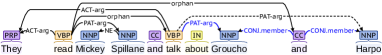
(a) PSD formalism of the example sentence

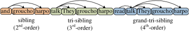
(b) Part of higher-order features

Figure 1: Part of $2^{nd}$-order, $3^{rd}$-order, $4^{th}$-order features appeared in the example sentence.

Several semantic dependency parsers are presented in recent years. Most of them are first-order parsers Du et al. (2015); Peng et al. (2017); Dozat and Manning (2018); Wang et al. (2018); Fernández-González and Gómez-Rodríguez (2020), the rest are second-order parsers Martins and others (2014); Cao et al. (2017); Wang et al. (2019), higher-order parsing remains under-explored yet. The reason for this issue is that modeling higher-order features with exact inference is NP-hard. Higher-order features have been widely exploited in syntactic dependency parsing Carreras (2007); Koo and Collins (2010); Ma and Zhao (2012); Ji et al. (2019); Zhang et al. (2020). However, most of the previous algorithms for higher-order syntactic dependency tree parsing are not applicable to semantic dependency graph parsing.

Graph neural networks (GNNs) have been demonstrated to be an effective tool for solving NP-hard problems with approximate inference in many graph learning tasks Prates et al. (2019); Zhang and Lee (2019); Zhao et al. (2021). GNNs aggregate higher-order information in a similar incremental manner: one GNN layer encodes information about immediate neighbors and $K$ layers encode $K$-order neighborhoods (i.e., information about nodes at most $K$ hops aways).

Inspired by the success of GNNs, we investigate building a higher-order semantic dependency parser (HOSDP) by applying GNNs in this paper. Instead of explicitly extracting higher-order features from intermediate parsing graphs, we aggregate higher-order information and bring global evidence into decoders’ final decision by stacking multiple GNN layers. We extend the biaffine parser Dozat and Manning (2018) and employ it as the vanilla parser to produce an initial adjacency matrix (close to gold) since there is no graph structure available during testing. Two GNNs variants, Graph Convolutional Network (GCN) Kipf and Welling (2016) and Graph Attention Network (GAT) Veličković et al. (2017) have been investigated in HOSDP. Our model has been evaluated on SemEval 2015 Task 18 English Dataset which contains three semantic dependency formalisms (DM, PAS, and PSD). Experimental results show that HOSDP outperforms the previous best one. In addition, HOSDP shows more advantage over the baseline in the longer sentence and PSD formalism (appearing linguistically most fine-grained). Our code is publicly available at https://github.com/LiBinNLP/HOSDP.

2 Related work

In this section, the studies of higher-order syntactic dependency parsing, semantic dependency parsing and GNNs will be summarized as follows.

2.1 Higher-order Syntactic Dependency Parsing

Higher-order parsing has received a lot of attention in the syntactic dependency parsing. Carreras (2007) presented a second parser which incorporate grand-parental relationships in the dependency structure. Koo and Collins (2010) developed a third-order parser. They introduced grand-sibling and tri-sibling parts. Ma and Zhao (2012) developed a forth-order parser which utilized grand-tri-sibling parts for fourth-order dependency parsing. Ji et al. (2019) used graph neural networks to captures higher-order information for syntactic dependency parsing, which was closely related to our work. Zhang et al. (2020) presented a second-order TreeCRF extension to the biaffine parser.

Higher-order features have been widely exploited in syntactic dependency parsing. However, most of the previous algorithms for higher-order syntactic dependency tree parsing are not applicable to semantic dependency graph parsing.

2.2 Semantic Dependency Parsing

Several SDP models are presented in the recent years. Their parsing mechanisms are either transition-based or graph-based. Most of them are first-order parsers. Wang et al. (2018) presented a neural transition-based parser, using a variant of list-based arc-eager transition algorithm for dependency graph parsing. Lindemann et al. (2020) developed a transition-based parser for Apply-Modify dependency parsing. They extended the stack-pointer model to predict transitions. Fernández-González and Gómez-Rodríguez (2020) developed a transition-based parser, using Pointer Network to choose a transition between Attach-p and Shift. More recently, there has been a predominance of purely graph-based SDP models. Dozat and Manning (2018) extended the LSTM-based syntactic parser of Dozat et al. (2017) to train on and generate SDG. Kurita and Søgaard (2019) developed a reinforcement learning-based approach that iteratively applies the syntactic dependency parser to build a DAG structure sequentially. Jia et al. (2020) presented a semi-supervised model based on Conditional Random Field Autoencoder to learn a dependency graph parser. He and Choi (2020) significantly improved the performance by introducing contextual string embeddings (called Flair).

Higher-order SDP receives less attention. Martins and others (2014) developed a second-order parser which employ a feature-rich linear model to incorporate first and second-order features (arcs, siblings, grandparents and co-parents). $AD^{3}$ algorithm was employed for approximate decoding. Cao et al. (2017) presented a quasi-second-order parser and used a dynamic programming algorithm (called Maximum Subgraph) for exact decoding. Wang et al. (2019) extended the parser Dozat and Manning (2018) and managed to add second-order information for score computation and then apply either mean-field variational inference or loopy belief propagation for approximate decoding.

Higher-order parsing remains under-explored yet. The reason for this issue is that modeling higher-order features with exact inference is NP-hard.

2.3 Graph Neural Networks

Recent years have witnessed great success from GNNs in graph learning. Two main families of GNNs have been proposed, i.e., spectral methods and spatial methods. GCNs Kipf and Welling (2016) is a spectral-based method, which learns node representation based on graph spectral theory. GAT Veličković et al. (2017) is a spatial-based method, which introduces the multi-head attention mechanism to learn different attention scores for neighbors when aggregating information.

GNNs have been demonstrated to be an effective tool for solving NP-hard problems with approximate inference in many graph learning tasks. Prates et al. (2019) utilized GNNs to solve the Traveling Salesperson Problem, a highly relevant NP-Complete problem. Zhang and Lee (2019) used GNNs to solve NP-hard assignment problems in image feature matching task. Zhao et al. (2021) used GCNs to solve maximum weighted independent set problem, which is NP-hard. Inspired by the success of GNNs, we investigate building a higher-order semantic dependency parser by applying GNNs.

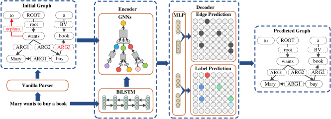
Figure 2: Overall architecture of the proposed HOSDP.

3 HOSDP

HOSDP is a parser extends Dozat and Manning (2018). An overview of HOSDP is shown as Figure 2. Given sentence $s$ with $n$ words $[w_{1},w_{2},\dots,w_{n}]$, there are three steps to parse it as an SDG. Firstly, the sentence will be parsed with a vanilla SDP parser, producing an initial SDG. Secondly, the contextualized word representations output by long short-term memory (BiLSTM) and adjacency matrix obtained from the initial SDG will be fed into the GNN encoder, to obtain node representations which aggregate higher-order information. Finally, MLP will be used to get the hidden state representation, and then decoded by biaffine classifier to predict edge and label.

3.1 Vanilla Parser

We use biaffine parser Dozat and Manning (2018) as the vanilla parser. The sentence $s$ will be parsed by the vanilla parser to obtain initial adjacency matrix.

$$(\tilde{A},\tilde{G})=VanillaParser(W,F)$$ (1)

where $\tilde{A}$ is the initial adjacency matrix; $\tilde{G}$ is the initial SDG; $W$ denotes $n$ words and $F$ denotes features of words.

3.2 Encoder

We concatenate word and feature embeddings, and feed them into a BiLSTM to obtain contextualized representations.

$$x_{i}=e_{i}^{(word)}\oplus e_{i}^{(feat)}$$ (2)

$$O=BiLSTM(X)$$ (3)

where $x_{i}$ is the concatenation ($\oplus$) of the word and feature embeddings of word $w_{i}$, $X$ represents $[x_{1},x_{2},\dots,x_{n}]$. $O=[o_{1},o_{2},\dots,o_{n}]$ is the contextualized representations of sequence $X$.

Then we employ $K$-layer GNNs to capture higher-order information by aggregating representation of $K$-order neighborhoods. Node embedding matrix $R^{(k)}$ in $k^{th}$-layer is computed as Equation 4:

$$R^{(k)}=\emph{GNNLayer}^{(k-1)}(R^{(k-1)},\tilde{A})$$ (4)

When GNNLayer is implemented in GCN, the representation of node $i$ in $k^{th}$ layer $r_{i}^{(k)}$ is computed as Equation 5

$$r_{i}^{(k)}=\sigma\left(W\sum_{j\in N(i)}r_{j}^{(k-1)}+Br_{i}^{(k-1)}\right)$$ (5)

where $W$ and $B$ are parameter matrices; $N(i)$ are neighbors of node $i$; $\sigma$ is active function (we use ReLU); $r_{i}^{(0)}=o_{i}$.

When GNNLayer is implemented in GAT, $r_{i}^{(k)}$ is computed as Equation 6:

$$r_{i}^{(k)}=\sigma\left(W\sum_{j\in N(i)}a_{ij}^{(m)(k-1)}r_{j}^{(k-1)}+Br_{i}^{(k-1)}\right)$$ (6)

where $a_{ij}^{(m)(k-1)}$ is attention coefficient of node $i$ to its neighbour $j$ in attention head $m$ at $(k-1)^{th}$ layer.

Although higher-order information is important, GNNs would suffer from the over-smoothing problem when the number of layer is too many. So we stack 3 layers with the past experience.

3.3 Decoder

Decoder has two modules: edge existence prediction module and edge label prediction module. For each of the two modules, we use MLP to split the final node representation $R=[r_{1},r_{2},\dots,r_{n}]$ into two parts—a head representation, and a dependent representation, as shown in Equation 7 to 10:

$$h_{i}^{(edge-head)}=MLP^{(edge-head)}(ri)$$ (7)

$$h_{i}^{(label-head)}=MLP^{(label-head)}(ri)$$ (8)

$$h_{i}^{(edge-dep)}=MLP^{(edge-dep)}(ri)$$ (9)

$$h_{i}^{(label-dep)}=MLP^{(label-dep)}(ri)$$ (10)

We can then use biaffine classifiers (as Equation 11), which are generalizations of linear classifiers to include multiplicative interactions between two vectors—to predict edges and labels, as Equation 12 and 13 :

$$Biaff(x_{1},x_{2})=x_{1}^{T}Ux_{2}+W(x_{1}\oplus x_{2})+b$$ (11)

$$s_{i,j}^{(edge)}=Biaff^{(edge)}(h_{i}^{(edge-dep)},h_{j}^{(edge-head)})$$ (12)

$$s_{i,j}^{(label)}=Biaff^{(label)}(h_{i}^{(label-dep)},h_{j}^{(label-head)})$$ (13)

where $s_{i,j}^{(edge)}$ and $s_{i,j}^{(label)}$ are scores of edge existence and edge label between the word $w_{i}$ and $w_{j}$. $U$, $W$ and $b$ are learned parameters of biffine classifier. For edge existence prediction module, $U$ will be $(d*1*d)$-dimensional, so that $s_{i,j}^{(edge)}$ will be a scalar. For edge label prediction, if the parser is unlabeled, $U$ will be $(d*1*d)$-dimensional, so that $s_{i,j}^{(label)}$ will be a scalar. If the parser is labeled, $U$ will be $(d*c*d)$-dimensional, where $c$ is the number of labels, so that $s_{i,j}^{(label)}$ is a vector that represents the probability distributions of each label.

The unlabeled parser scores each edge between pairs of words in the sentence—these scores can be decoded into a graph by keeping only edges that received a positive score. The labeled parser scores every label for each pair of words, so we simply assign each predicted edge its highest-scoring label and discard the rest.

$$\hat{y}_{i,j}^{(edge)}=\{s_{i,j}^{(edge)}>0\}$$ (14)

$$\hat{y}_{i,j}^{(label)}=\arg\max s_{i,j}^{(label)}$$ (15)

3.4 Learning

We can train the system by summing the losses from the two modules, back propagating error to the parser. Cross entropy function is used as as the loss function, which is computed as Equation 16:

$$CE(p,q)=-\sum_{x}p(x)\log q(x)$$ (16)

We define the loss function of edge existence prediction module and edge label prediction module:

$$\mathcal{L}^{(edge)}(\theta_{2})=CE(\hat{y}_{i,j}^{(edge)},y_{i,j}^{(edge)})$$ (17)

$$\mathcal{L}^{(label)}(\theta_{1})=CE(\hat{y}_{i,j}^{(label)},y_{i,j}^{(label)})$$ (18)

where $\theta_{1}$ and $\theta_{2}$ are the parameters of two modules.

Then the Adaptive Moment Estimation (Adam) method is used to optimize the summed loss function $\mathcal{L}$:

$$\mathcal{L}=\lambda\mathcal{L}^{(edge)}+(1-\lambda)\mathcal{L}^{(label)}$$ (19)

where $\lambda$ is a tunable interpolation constant $\lambda\in(0,1)$.

4 Experiments

4.1 Dataset

To evaluate the performance of HOSDP, we conduct experiments on the SemEval 2015 Task 18 English datasets Oepen et al. (2015), where all sentences are annotated with three different formalisms: DELPH-IN MRS (DM), Predicate-Argument Structure (PAS) and Prague Semantic Dependencies (PSD). We use the same dataset split as in previous approaches Almeida and Martins (2015); Du et al. (2015) with 33,964 training sentences from Sections 00-19 of the Wall Street Journal corpus Marcus et al. (1993), 1,692 development sentences from Section 20, 1,410 sentences from Section 21 as in-domain (ID) test set, and 1,849 sentences sampled from the Brown Corpus Francis and Kucera (1982) as out-of-domain (OOD) test data. For the evaluation, we use the evaluation script used in Wang et al. (2019), reporting labelled F-measure scores (LF1) (including ROOT arcs) on the ID and OOD test sets for each formalism as well as the macro-average over the three of them.

4.2 Hyperparameters

The hyperparameter configuration for our final system is given in Appendix A. We use 100-dimensional pretrained GloVe embeddings. Only words or lemmas that occurred 7 times or more are included in the word and lemma embedding matrix—including less frequent words appeared to facilitate overfitting. Character-level word embeddings are generated using a one-layer unidirectional LSTM that convolved over three character embeddings at a time, whose final state is linearly transformed to be 100-dimensional.

We train the model for at most 100 epochs and terminated training early after 20 epochs with no improvement on the development set.

Models	DM		PAS		PSD		Avg
	ID	OOD	ID	OOD	ID	OOD	ID	OOD
Du et al. Du et al. (2015)	89.1	81.8	91.3	87.2	75.7	73.3	85.3	80.8
A&M Almeida and Martins (2015)	88.2	81.8	90.9	86.9	76.4	74.8	85.2	81.2
PTS17 Peng et al. (2017): Basic	89.4	84.5	92.2	88.3	77.6	75.3	86.4	82.7
PTS17 Peng et al. (2017): Basic	90.4	85.3	92.7	89.0	78.5	76.4	87.2	83.6
WCGL Wang et al. (2018)	90.3	84.9	91.7	87.6	78.6	75.9	86.9	82.8
D&M Dozat and Manning (2018): Basic	91.4	86.9	93.9	90.8	79.1	77.5	88.1	85.0
MF Wang et al. (2019): Basic	93.0	88.4	94.3	91.5	80.9	78.9	89.4	86.3
LBP Wang et al. (2019): Basic	92.9	88.4	94.3	91.5	81.0	78.8	89.4	86.2
Lindemann et al. Lindemann et al. (2019): Basic	91.2	85.7	92.2	88.0	78.9	76.2	87.4	83.3
Semantic Pointer Fernández-González and Gómez-Rodríguez (2020): Basic	92.5	87.7	94.2	91.0	81.0	78.7	89.2	85.8
HOSDP (GCN): Basic	93.3	88.0	94.8	91.1	85.6	83.6	91.2	87.6
HOSDP (GAT): Basic	93.0	87.9	94.8	91.6	85.4	83.3	91.1	87.6
D&M Dozat and Manning (2018): +Char+Lemma	93.7	88.9	93.9	90.6	81.0	79.4	89.5	86.3
MF Wang et al. (2019): +Char+Lemma	94.0	89.7	94.1	91.3	81.4	79.6	89.8	86.9
LBP Wang et al. (2019): +Char+Lemma	93.9	89.5	94.2	91.3	81.4	79.5	89.8	86.8
Jia et al. Jia et al. (2020): +Lemma	93.6	89.1	-	-	-	-	-	-
Semantic Pointer Fernández-González and Gómez-Rodríguez (2020): +Char+Lemma	93.9	89.6	94.2	91.2	81.8	79.8	90.0	86.9
HOSDP (GCN): +Char+Lemma	94.2	90.1	94.9	91.4	86.4	84.9	91.8	88.8
HOSDP (GAT): +Char+Lemma	94.4	89.9	95.0	91.8	86.2	84.6	91.9	88.8
Lindemann et al. Lindemann et al. (2019): +BERTlarge	94.1	90.5	94.7	92.8	82.1	81.6	90.3	88.3
Lindemann et al. Lindemann et al. (2020): +BERTlarge	93.9	90.4	94.7	92.7	81.9	81.6	90.2	88.2
Semantic Pointer Fernández-González and Gómez-Rodríguez (2020): +Char+Lemma+BERTbase	94.4	91.0	95.1	93.4	82.6	82.0	90.7	88.8
He et al. He and Choi (2020): +Char+Lemma+BERTbase+Flair	94.6	90.8	96.1	94.4	86.8	79.5	92.5	88.2
HOSDP (GCN): +Char+Lemma+BERTbase	95.1	91.1	95.7	93.2	87.7	87.3	92.8	90.5
HOSDP (GAT): +Char+Lemma+BERTbase	95.3	91.9	96.0	94.3	87.0	86.7	92.8	91.0

Table 1: Comparison of labeled F1 scores achieved by our model and previous state-of-the-art. The F1 scores of Baseline and our models are averaged over 5 runs. ID denotes the in-domain (WSJ) test set and OOD denotes the out-of-domain (Brown) test set. +Char, +Lemma, +BERT, and +Flair mean augmenting the token embeddings with character-level, lemma embeddings, BERT embeddings, and Flair embeddings. Semi-SDP only shows the full-supervised result on DM formalism.

4.3 Baseline

We compare HOSDP with previous state-of-the-art parsers in Table 1. Du et al. (2015) is a hybrid model. A&M is from Almeida and Martins (2015). WCGL Wang et al. (2018) is a neural transition-based model. PTS17 proposed by Peng et al. (2017) and Basic is single task parsing while Freda3 is a multitask parser across three formalisms. D&M Dozat and Manning (2018) is a first-order graph-based model. MF and LBP Wang et al. (2019) are a second-order model using mean field variational inference or loopy belief propagation. Lindemann et al. (2019) and Lindemann et al. (2020) are compositional semantic parser for SDP and abstract meaning representation. Semantic Pointer Fernández-González and Gómez-Rodríguez (2020) is a transition-based model using Pointer Network. Jia et al. (2020) is a semi-supervised parser, only the full-supervised result on DM formalism is shown in their paper. He and Choi (2020) uses not only BERT but also contextual string embeddings (called Flair).

4.4 Main Results

We group SDP models in three blocks depending on the embeddings provided to the models: (1) just basic pre-trained GloVe word embeddings and POS tag embeddings (Basic), (2) character and pre-trained lemma embeddings augmentation (+Char+Lemma) and (3) pre-trained BERT embeddings augmentation (+Char+Lemma+BERT).

Table 1 presents the comparison of HOSDP and related studies on the test sets of SemEval 2015 Task 18 English datasets. From the results, we have the following observations:

• In the basic setting, HOSDP achieves 1.8 and 1.3 averaged LF1 improvements on the ID and OOD test set over the previous best parsers.

• Adding both the character-level and the lemma embeddings, most models improve performance quite a bit generally. HOSDP leads to 1.9 and 1.9 averaged LF1 improvements over the previous best parsers on the ID and OOD test sets.

• Adding BERT embedding pushes performance even higher generally. HOSDP outperforms the previous best parsers by 0.3 and 2.2 average LF1 improvements on ID and OOD test sets, respectively.

• HOSDP makes significant improvements on the PSD formalism, with 4.6 and 4.7 LF1 improvements in the basic setting, 4.6 and 5.1 LF1 improvements when character-level and lemma embeddings are added, 0.9 and 5.3 LF1 improvements when BERT embeddings are added on the ID and OOD test sets, respectively.

• The LF1 scores of all parsers on the PSD is lower than the other two formalisms. Table 2 shows part of contrastive statistics of three formalisms. We have noticed that PSD formalism appears linguistically most fine-grained because it contains the most semantic labels and frames Oepen et al. (2015). This makes PSD more challenging to predict. However, HOSDP performs better than other first-order and second-order parsers, suggesting that higher-order information is beneficial to SDP.

• The performances of HOSDP (GCN) and HOSDP (GAT) are almost the same in three embedding settings, demonstrating that both GCNs and GAT are capable to capture higher-order information.

In summary, outstanding performances of HOSDP have demonstrated that higher-order information can bring considerable accuracy gains in SDP. In addition, GNNs are capable to capture higher-order information and are effective for higher-order modeling.

	DM		PAS		PSD
	ID	OOD	ID	OOD	ID	OOD
# labels	59	47	42	41	91	74
# frames	297	172	-	-	5426	1208

Table 2: Contrastive statistics of three semantic formalisms.

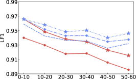
(a) DM.ID

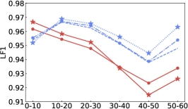
(b) PAS.ID

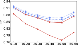
(c) PSD.ID

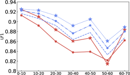
(d) DM.OOD

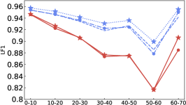
(e) PAS.OOD

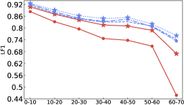
(f) PSD.OOD

Figure 3: LF1 of different sentence lengths in 3 formalisms. $\star$-T represents that only the POS tag is used as feature. $\star$-TCL represents that the POS tag, character-level and lemma embeddings are used as features. $\star$-TCLB represents that the POS tag, character-level, lemma and BERT embeddings are used as features.

4.5 Analysis

Performance on Different Sentence Length

We want to study the impact of sentence lengths. The ID and OOD test sets of the three formalisms are split with 10 tokens range. The ID test set has 6 groups and OOD has 7. HOSDP (GCN) and biaffine parser are evaluated on them. The results on diffenent groups are shown in Figure 3.

The results show that HOSDP outperforms the biaffine parser on different groups with the same embedding configuration, except for slightly lower on the first group (0-10 tokens) on ID test set of PAS formalism. Furthermore, HOSDP that only utilizes POS tag embedding outperforms biaffine parse that uses POS tag, character-level, and lemma embeddings, when sentences get longer, especially when sentences are longer than 30. It turns out that higher-order information is favorable for longer sentences since higher-order dependency relationships are more prevalent in longer sentences.

Case study

We provide a parsing example to show why HOSDP benefits from higher-order information. Figure 4 shows the parsing results of biaffine parser (Figure 4(a)) and HOSDP (GCN) (Figure 4(b)), for sentence (sent_id=40504035, in OOD of PSD formalism): There is never enough corn, peas or strawberries. Both of two parsers are trained in the basic embedding setting.

In the gold annotation, three words corn, peas and strawberries are three members of the disjunctive word or. In addition, the word enough has three dependency edges labeled EXT with them. In the result of biaffine parser, only dependency edge between enough and corn is identified, the remaining two are not. In HOSDP (GCN), given the initial SDG predicted by biaffine parser, words corn, peas and strawberries aggregate the higher-order information of or and is ($1^{st}$-order), there ($2^{nd}$-order) and ROOT ($3^{rd}$-order). The word enough aggregate the higher-order information of the corn ($1^{st}$-order), is and or ($2^{nd}$-order), there ($3^{rd}$-order), and ROOT ($4^{th}$-order). Dependent-word enough and three head-words corn, peas and strawberries aggregate information of four common words (ROOT, There, is and or). Therefore the representations of them with higher-order information bring global evidence into decoders’ final decision. As a result, it is effortless for HOSDP to identify that there are also two dependency edges labeled EXT between dependent-word enough and head-words peas and strawberries.

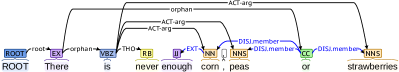
(a) Parsing result of biaffine parser

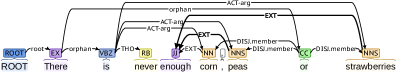
(b) Parsing result of HOSDP (GCN)

Figure 4: Parsing results of biaffine parser and HOSDP, for the sentence (sent_id=40504035 in OOD of PSD formalism). Some irrelevant dependency edges are hidden.

5 Conclusions

We propose a higher-order semantic dependency parser, which employs the GNNs to capture higher-order information. Experimental results show that HOSDP outperforms previous best one on the SemEval 2015 Task 18 English datasets. In addition, HOSDP shows more advantage in longer sentence and complex semantic formalism. In the future, we would like to apply graph structure learning models to learn adjacency matrix, rather than depending on the results of vanilla parser.

Appendix A Hyperparameter values

Layer	Hyper-parameter	Value
Input	Glove/POS/Lemma/Char/BERT	100
LSTM	layers	3
	hidden size	400
	dropout	0.33
GNN	GCN layers	3
	GAT heads	8
	GAT $\alpha$	0.2
	GCN/GAT dropout	0.33
MLP	edge-head/label-head hidden size	600
	edge-dep/label-dep hidden size	600
Trainer	optimizer	Adam
	learning rate	$1e^{-2}$
	Adam ($\beta_{1}$, $\beta_{2}$)	(0.95, 0.95)
	decay rate	0.75
	decay step length	5000
	$\lambda$	0.1

Table 3: Final hyperparameter configuration.

References

- Almeida and Martins [2015] Mariana SC Almeida and André FT Martins. Lisbon: Evaluating turbo semantic parser on multiple languages and out-of-domain data. In Proceedings of the 9th International Workshop on Semantic Evaluation (SemEval 2015), pages 970–973, 2015.
- Cao et al. [2017] Junjie Cao, Sheng Huang, Weiwei Sun, and Xiaojun Wan. Quasi-second-order parsing for 1-endpoint-crossing, pagenumber-2 graphs. In Proceedings of the 2017 Conference on Empirical Methods in Natural Language Processing, pages 24–34, 2017.
- Carreras [2007] Xavier Carreras. Experiments with a higher-order projective dependency parser. In Proceedings of the 2007 Joint Conference on Empirical Methods in Natural Language Processing and Computational Natural Language Learning (EMNLP-CoNLL), pages 957–961, 2007.
- Dozat and Manning [2018] Timothy Dozat and Christopher D Manning. Simpler but more accurate semantic dependency parsing. arXiv preprint arXiv:1807.01396, 2018.
- Dozat et al. [2017] Timothy Dozat, Peng Qi, and Christopher D Manning. Stanford’s graph-based neural dependency parser at the conll 2017 shared task. In Proceedings of the CoNLL 2017 Shared Task: Multilingual Parsing from Raw Text to Universal Dependencies, pages 20–30, 2017.
- Du et al. [2015] Yantao Du, Fan Zhang, Xun Zhang, Weiwei Sun, and Xiaojun Wan. Peking: Building semantic dependency graphs with a hybrid parser. In Proceedings of the 9th international workshop on semantic evaluation (semeval 2015), pages 927–931, 2015.
- Fernández-González and Gómez-Rodríguez [2020] Daniel Fernández-González and Carlos Gómez-Rodríguez. Transition-based semantic dependency parsing with pointer networks. arXiv preprint arXiv:2005.13344, 2020.
- Francis and Kucera [1982] Winthrop Nelson Francis and Henry Kucera. Frequency analysis of English usage: Lexicon and usage. Houghton Mifflin, 1982.
- He and Choi [2020] Han He and Jinho Choi. Establishing strong baselines for the new decade: Sequence tagging, syntactic and semantic parsing with bert. In The Thirty-Third International Flairs Conference, 2020.
- Ji et al. [2019] Tao Ji, Yuanbin Wu, and Man Lan. Graph-based dependency parsing with graph neural networks. In Proceedings of the 57th Annual Meeting of the Association for Computational Linguistics, pages 2475–2485, 2019.
- Jia et al. [2020] Zixia Jia, Youmi Ma, Jiong Cai, and Kewei Tu. Semi-supervised semantic dependency parsing using crf autoencoders. In Proceedings of the 58th Annual Meeting of the Association for Computational Linguistics, pages 6795–6805, 2020.
- Kipf and Welling [2016] Thomas N Kipf and Max Welling. Semi-supervised classification with graph convolutional networks. arXiv preprint arXiv:1609.02907, 2016.
- Koo and Collins [2010] Terry Koo and Michael Collins. Efficient third-order dependency parsers. In Proceedings of the 48th Annual Meeting of the Association for Computational Linguistics, pages 1–11, 2010.
- Kurita and Søgaard [2019] Shuhei Kurita and Anders Søgaard. Multi-task semantic dependency parsing with policy gradient for learning easy-first strategies. arXiv preprint arXiv:1906.01239, 2019.
- Lindemann et al. [2019] Matthias Lindemann, Jonas Groschwitz, and Alexander Koller. Compositional semantic parsing across graphbanks. arXiv preprint arXiv:1906.11746, 2019.
- Lindemann et al. [2020] Matthias Lindemann, Jonas Groschwitz, and Alexander Koller. Fast semantic parsing with well-typedness guarantees. arXiv preprint arXiv:2009.07365, 2020.
- Ma and Zhao [2012] Xuezhe Ma and Hai Zhao. Fourth-order dependency parsing. In Proceedings of COLING 2012: posters, pages 785–796, 2012.
- Marcus et al. [1993] Mitchell Marcus, Beatrice Santorini, and Mary Ann Marcinkiewicz. Building a large annotated corpus of english: The penn treebank. 1993.
- Martins and others [2014] André FT Martins et al. Priberam: A turbo semantic parser with second order features. 2014.
- Oepen et al. [2015] Stephan Oepen, Marco Kuhlmann, Yusuke Miyao, Daniel Zeman, Silvie Cinková, Dan Flickinger, Jan Hajic, and Zdenka Uresova. Semeval 2015 task 18: Broad-coverage semantic dependency parsing. In Proceedings of the 9th International Workshop on Semantic Evaluation (SemEval 2015), pages 915–926, 2015.
- Peng et al. [2017] Hao Peng, Sam Thomson, and Noah A Smith. Deep multitask learning for semantic dependency parsing. arXiv preprint arXiv:1704.06855, 2017.
- Prates et al. [2019] Marcelo Prates, Pedro HC Avelar, Henrique Lemos, Luis C Lamb, and Moshe Y Vardi. Learning to solve np-complete problems: A graph neural network for decision tsp. In Proceedings of the AAAI Conference on Artificial Intelligence, volume 33, pages 4731–4738, 2019.
- Veličković et al. [2017] Petar Veličković, Guillem Cucurull, Arantxa Casanova, Adriana Romero, Pietro Lio, and Yoshua Bengio. Graph attention networks. arXiv preprint arXiv:1710.10903, 2017.
- Wang et al. [2018] Yuxuan Wang, Wanxiang Che, Jiang Guo, and Ting Liu. A neural transition-based approach for semantic dependency graph parsing. In Proceedings of the AAAI Conference on Artificial Intelligence, volume 32, 2018.
- Wang et al. [2019] Xinyu Wang, Jingxian Huang, and Kewei Tu. Second-order semantic dependency parsing with end-to-end neural networks. arXiv preprint arXiv:1906.07880, 2019.
- Zhang and Lee [2019] Zhen Zhang and Wee Sun Lee. Deep graphical feature learning for the feature matching problem. In Proceedings of the IEEE/CVF International Conference on Computer Vision, pages 5087–5096, 2019.
- Zhang et al. [2020] Yu Zhang, Zhenghua Li, and Min Zhang. Efficient second-order treecrf for neural dependency parsing. arXiv preprint arXiv:2005.00975, 2020.
- Zhao et al. [2021] Zhongyuan Zhao, Gunjan Verma, Chirag Rao, Ananthram Swami, and Santiago Segarra. Distributed scheduling using graph neural networks. In ICASSP 2021-2021 IEEE International Conference on Acoustics, Speech and Signal Processing (ICASSP), pages 4720–4724. IEEE, 2021.