Abstract: This paper studies limit measures of stationary measures of stochastic ordinary differential equations on the Euclidean space and tries to determine which invariant measures of an unperturbed system will survive. Under the assumption for SODEs to admit the Freidlin–Wentzell or Dembo–Zeitouni large deviations principle with weaker compactness condition, we prove that limit measures are concentrated away from repellers which are topologically transitive, or equivalent classes, or admit Lebesgue measure zero. We also preclude concentrations of limit measures on acyclic saddle or trap chains. This illustrates that limit measures are concentrated on Liapunov stable compact invariant sets. Applications are made to the Morse–Smale systems, the Axiom A systems including structural stability systems and separated star systems, the gradient or gradient-like systems, those systems possessing the Poincaré–Bendixson property with a finite number of limit sets to obtain that limit measures live on Liapunov stable critical elements, Liapunov stable basic sets, Liapunov stable equilibria and Liapunov stable limit sets including equilibria, limit cycles and saddle or trap cycles, respectively. A number of nontrivial examples admitting a unique limit measure are provided, which include monostable, multistable systems and those possessing infinite equivalent classes.

AMS Subject Classification:  Primary 60H10,37B35,60B10; Secondary 60F10, 37A50, 37C70.

Keywords: large deviations; stationary measure; limit measure; concentration; Morse-Smale system; Axiom A system; gradient-like system; Poincaré-Bendixson property.

1 Introduction

This paper studies limit measures and their supports of stationary measures for stochastic ordinary differential equations

$$\mathrm{d}X^{\varepsilon}_{t}=b(X^{\varepsilon}_{t})\mathrm{d}t+\varepsilon\sigma(X^{\varepsilon}_{t})\mathrm{d}w_{t},\quad X^{\varepsilon}_{0}=x\in\mathbb{R}^{r}$$ (1.1)

when $\varepsilon$ goes to zero, where $w_{t}=(w^{1}_{t},\cdots,w^{r}_{t})^{*}$ is a standard $r$-dimensional Wiener process, the diffusion matrix $a=(a_{ij})_{r\times r}=\sigma\sigma^{*}$ is positive definite, which is called to be nondegenerate, where ^∗ denotes transpose. System (1.1) is regarded as a stochastic perturbation of the deterministic dynamical system

$$\frac{\mathrm{d}x}{\mathrm{d}t}=b(x),\quad x(0)=x\in\mathbb{R}^{r}.$$ (1.2)

This asymptotic problem was first proposed by Kolmogorov in the 1950s (see [35, p.838]). Khasminskii [21] proved that a stationary measure of a Markov process on a torus converges weakly to an invariant measure for a dynamical system on the torus as diffusion term tends to zero, hence he has been regarded as the first one to realize that limit measures of stationary measures are invariant measures for unperturbed systems. Using large deviations principle, Freidlin and Wentzell solved the problem of rough asymptotics of stationary measures of a diffusion process with small diffusion on a compact connected manifold [40, 11]. Precisely, under assumptions that there are a finite number of equivalent classes containing all limit sets of the unperturbed system, they created a method to determine which stable equivalent class or classes a limit measure of stationary measures is concentrated on after a series of rare probability estimates. Kifer [22] generalized the corresponding results of Freidlin and Wentzell to discrete-time dynamical systems on a compact manifold with small unbounded random perturbations satisfying large deviations principle. Ruelle [31] verified that limit measures of stationary measures for discrete-time dynamical systems with small bounded random perturbations live on quasiattractors. Benaïm [1] investigated the dynamical properties of a class of urn processes and recursive stochastic algorithms with constant gain and proved that limit measures of the process are concentrated on the Birkhoff center of irreducible attractors of its averaging ordinary differential equations.

As for stochastic system (1.1) on the Euclidean space, Freidlin and Wentzell [11] and Hwang [19] considered gradient systems (that is, $b(x)=-\nabla U(x)$) perturbed by an additive noise and showed that limit measures of stationary measures have their supports on the lowest energy points via the large deviation technique and Laplace’s method, respectively. Huang et al. [18] proved that all limit measures of stationary measures of (1.1) are invariant with respect to the solution flow of (1.2) and sit on the global attractor of (1.2) by estimating measure values of regular stationary measures in an exterior domain with respect to diffusion and Liapunov-like functions. For a given deterministic ODEs (1.2) with a strongly local attractor (repeller), they constructed a nondegenerate diffusion $\sigma$ such that limit measures of (1.1) are concentrated on the local attractor (away from the local repeller); then Ji et al. [20] removed the “strong” hypothesis of attractor and repeller and obtained the same conclusion. Besides, Huang et al. [18] proved all limit measures of (1.1) for all small nondegenerate diffusion perturbations are concentrated away from any hyperbolic repelling equilibrium by constructing a positive definite quadratic form as an anti-Liapunov function. Chen, Dong and Jiang [4] presented a criterion that limit measures are concentrated away from repellers, which can be applied to repelling limit cycles or quasi-periodic orbits. For a gradient system (1.2), Huang et al. [17] proved all limit measures of (1.1) for all small nondegenerate diffusion perturbations support on the set of critical points of the potential function $U$. Chen et al. [7] analyzed limit measures of one dimensional system (1.1) as the white noise vanishes and proved that all limit measures are exactly concentrated on the global minimizers of $-\int\frac{b(u)}{\sigma^{2}(u)}\mathrm{d}u$ if $b^{\prime}(x)\neq 0$ at all these global minimizers. This shows that the limit measure may support on those lesser stable equilibria but with smaller $\sigma$.

Under the assumptions that stochastic system (1.1) admits the Freidlin–Wentzell or Dembo–Zeitouni large deviations principle with weaker compactness condition, we shall exploit limit measures of stationary measures of stochastic ordinary differential equations (1.1). Such measures are more stable than other invariant measures of unperturbed systems (1.2) or the most stable if they uniquely exist to stochastic perturbations. We shall prove that limit measures are concentrated away from repellers which are topologically transitive, or equivalent classes, or admit Lebesgue measure zero. We also preclude concentrations of limit measures on acyclic saddle or trap chains. This shows that limit measures are concentrated on Liapunov stable compact invariant sets. Applications are made to the Morse–Smale systems, the Axiom A systems including structural stability systems and separated star systems, the gradient or gradient-like systems, those systems possessing the Poincaré–Bendixson property with a finite number of limit sets to obtain that limit measures live on Liapunov stable critical elements, Liapunov stable basic sets, Liapunov stable equilibria and Liapunov stable limit sets including equilibria, limit cycle and saddle or trap cycles, respectively. As far as we know, there are seldom examples of SODEs (1.1) on the Euclidean space whose limiting measures and their supports are clearly described. In Section 5, a number of nontrivial examples admitting a unique limit measure are provided, which include monostable, multistable systems and those possessing infinite equivalent classes.

2 Preliminaries and Notations

In this section, we recall some basic definitions and preliminary results from [40, 11, 22, 8, 9, 31, 27, 39, 14]. Throughout this paper we always assume that the coefficients $b$ and $\sigma$ are locally Lipschitz continuous on $\mathbb{R}^{r}$, the solutions of (1.1) and (1.2) are defined on $[0,+\infty)$, and the diffusion matrix $a=\sigma\sigma^{*}$ is nondegenerate on $\mathbb{R}^{r}$.

For $x\in\mathbb{R}^{r},\delta>0$ and $\mathcal{S},\mathcal{T}\subset\mathbb{R}^{r}$, we may write $B(x,\delta)=B_{\delta}(x)=\{y\in\mathbb{R}^{r}:|y-x|<\delta\}$, $\bar{B}_{\delta}(x)=\{y\in\mathbb{R}^{r}:|y-x|\leq\delta\}$, ${\rm dist}(\mathcal{S},\mathcal{T})=\inf_{y\in\mathcal{S},z\in\mathcal{T}}|y-z|$ and $(\mathcal{S})_{\delta}=\{y\in\mathbb{R}^{r}:{\rm dist}(y,\mathcal{S})<\delta\}$. Here $|\cdot|$ denotes the usual Euclidean norm.

We recall some standard definitions and results of dynamical systems (see, e.g., [31, 1, 27, 39, 14]). The solution semiflow of deterministic system (1.2) is denoted by $\Psi_{t}(x)=\Psi(t,x)$, its positive (resp. negative, entire) orbit is denoted by $\gamma^{+}(x)$ (resp. $\gamma^{-}(x),\gamma(x)$), and $\omega$-limit set (resp. $\alpha$-limit set) is denoted by $\omega(x)$ (resp. $\alpha(x)$).

For $D\subset\mathbb{R}^{r}$ and $T\geq 0$, let $\gamma^{+}(D)$ denote the sum of all positive orbits passing through points in $D$, the notations $\Psi_{T}(D)$ and $\Psi([0,T]\times D)$ are defined in a similar manner. A set $\Lambda\subset\mathbb{R}^{r}$ is positively invariant if $\Psi_{t}(\Lambda)\subset\Lambda$ for all $t\geq 0$. It is invariant if $\Psi_{t}(\Lambda)=\Lambda$ for all $t\geq 0$.

A set $\Lambda\subset\mathbb{R}^{r}$ is called topologically transitive (resp. minimal) for $\Psi$ if $\Lambda$ is nonempty compact invariant, and $\exists x\in\Lambda$ (resp. $\forall x\in\Lambda$) such that $\overline{\gamma^{+}(x)}=\Lambda$. Obviously, any minimal set is topologically transitive from the definitions. Suppose that $\Lambda$ is topologically transitive. Then it follows from the definition that for all open sets $U_{1}$ and $U_{2}$ in $\mathbb{R}^{r}$ such that $U_{1}\cap\Lambda$ and $U_{2}\cap\Lambda$ are nonempty, there is $T>0$ such that $\Psi_{T}(U_{1})\cap U_{2}\neq\emptyset$.

A subset $\mathcal{R}\subset\mathbb{R}^{r}$ is called to be a repeller (an attractor) for $\Psi$ provided: (i) $\mathcal{R}$ is nonempty, compact and invariant; and (ii) $\mathcal{R}$ has a neighborhood $N\subset\mathbb{R}^{r}$, called a fundamental neighborhood of $\mathcal{R}$, such that $\lim_{t\rightarrow-\infty}{\rm dist}\big{(}\Psi_{t}(x),\mathcal{R}\big{)}=0$ ($\lim_{t\rightarrow+\infty}{\rm dist}\big{(}\Psi_{t}(x),\mathcal{R}\big{)}=0$) uniformly in $x\in N$. In the case of attractor, we call $\mathcal{R}$ to be Liapunov stable.

Proposition 2.1.

Let $\mathcal{R}$ be a repeller for $\Psi$ with a fundamental neighborhood $N$. Then for any compact set $K\subset N\backslash\mathcal{R}$, there exists $T>0$ such that $\Psi_{t}(K)\subset N^{c}$ for all $t\geq T$.

Proof.

Let $K\subset N\backslash\mathcal{R}$ be a compact set. Then $d:={\rm dist}(K,\mathcal{R})>0$. Choose $\eta\in(0,d)$. Then $(\mathcal{R})_{\eta}\subset K^{c}$. Since $\mathcal{R}$ is a repeller, there is a $T>0$ such that for any $t\geq T$, $\Psi_{-t}(N)\subset(\mathcal{R})_{\eta}\subset K^{c}$. This implies that $N\subset\Psi_{t}(K^{c})$ for any $t\geq T$. Therefore, $\Psi_{t}(K)\subset N^{c}$ for any $t\geq T$. ∎

The dynamical system $\Psi$ on $\mathbb{R}^{r}$ is called dissipative if there exists a bounded set $B\subset\mathbb{R}^{r}$ with the property that for every compact $K\subset\mathbb{R}^{r}$ there exists $T=T(K)>0$ such that $\Psi_{t}(K)\subset B$ for all $t\geq T$. It is well known that the above dissipativity of $\Psi$ is equivalent to that $\Psi$ has a global attractor $\mathcal{A}$, that is, $\mathcal{A}$ is an attractor whose basin is all the space $\mathbb{R}^{r}$.

We now review some notions and properties in the large deviation theory, which are useful in deal with stationary measure asymptotics for small noise Markov processes (see, e.g., [40, 11, 22]).

For each fixed $T>0$, let ${\bf C}_{T}=C([0,T],\mathbb{R}^{r})$ (resp. ${\bf AC}_{T}=AC([0,T],\mathbb{R}^{r})$) denote the set of continuous functions (resp. absolutely continuous functions) on $[0,T]$ with values in $\mathbb{R}^{r}$. For $\varphi,\psi\in{\bf C}_{T}$ and $W\subset{\bf C}_{T}$, let $\rho_{T}(\varphi,\psi)=\sup_{0\leq t\leq T}|\varphi(t)-\psi(t)|$ and $\rho_{T}(\varphi,W)=\inf_{\phi\in W}\rho_{T}(\varphi,\phi)$. We define the following functional on ${\bf C}_{T}$:

$$S_{T}(\varphi)=S_{0T}(\varphi)=\left\{\begin{array}[]{ll}\frac{1}{2}\int\limits_{0}^{T}\Big{(}\dot{\varphi}(t)-b(\varphi(t))\Big{)}^{*}a^{-1}\big{(}\varphi(t)\big{)}\Big{(}\dot{\varphi}(t)-b(\varphi(t))\Big{)}{\rm d}t,&\hbox{if $\varphi\in{\bf AC}_{T}$,}\\ +\infty,&\hbox{otherwise.}\end{array}\right.$$ (2.3)

Let $X^{\varepsilon,x}_{\cdot}$, parametrized by $x\in\mathbb{R}^{r}$ and $\varepsilon>0$, be the solution of SDEs (1.1). For each $T>0$, $\varepsilon>0$ and $x\in\mathbb{R}^{r}$, one can regard $X^{\varepsilon,x}$ as a ${\bf C}_{T}$-valued random variable. Furthermore, to emphasize the dependence of initial conditions $x$, we also introduce the following notions $\ {\bf C}_{T}^{x}=\{\varphi\in{\bf C}_{T}:\varphi_{0}=x\},{\bf AC}_{T}^{x}=\{\varphi\in{\bf AC}_{T}:\varphi_{0}=x\}$, and functional $S_{T}^{x}$ on ${\bf C}_{T}$ :

$$S_{T}^{x}(\varphi)=S_{0T}^{x}(\varphi)=\left\{\begin{array}[]{ll}\frac{1}{2}\int\limits_{0}^{T}\Big{(}\dot{\varphi}(t)-b(\varphi(t))\Big{)}^{*}a^{-1}\big{(}\varphi(t)\big{)}\Big{(}\dot{\varphi}(t)-b(\varphi(t))\Big{)}{\rm d}t,&\hbox{if $\varphi\in{\bf AC}_{T}^{x}$,}\\ +\infty,&\hbox{otherwise.}\end{array}\right.$$ (2.4)

By the definition of $S_{T}^{x}$ in (2.4) we easily have the following assertion.

Remark 1.

$S_{0T}^{x}(\varphi)=0$ if and only if $\varphi$ (up to time $T$) coincides with the solution $\Psi_{\cdot}(x)$ of the deterministic system (1.2).

We give several definitions of uniform large deviations principles that are found in the literature. Let $\mathcal{K}$ be a collection of all compact subsets of $\mathbb{R}^{r}$ and $\mathbb{F}_{T}^{x}(s)=\{\varphi\in{\bf C}_{T}^{x}:S_{0T}^{x}(\varphi)\leq s\}$ for $T>0,x\in\mathbb{R}^{r},s\geq 0$. The first definition of a uniform large deviations principle presented here is due to Freidlin–Wenztell [40] (see also [11, p.74]).

Definition 2.1 (Freidlin–Wentzell uniform large deviations principle over $\mathcal{K}$).

For any fixed $T>0$, we say that the random variables $\{X^{\varepsilon,x}\}$ satisfy a Freidlin–Wentzell uniform large deviations principle with respect to the functionals $S_{T}^{x}$ uniformly over $\mathcal{K}$, if

${\bf(I_{u})}$ for each $s_{0}>0,\ \delta>0,\ \gamma>0$ and $K\in\mathcal{K}$ there exists $\varepsilon_{0}>0$ such that

$$\mathbb{P}_{x}\{\rho_{T}(X^{\varepsilon},\varphi)<\delta\}\geq\exp\{-\varepsilon^{-2}\big{(}S_{T}(\varphi)+\gamma\big{)}\}$$ (2.5)

for all $\varepsilon\in(0,\varepsilon_{0}],\ x\in K$ and $\varphi\in\mathbb{F}_{T}^{x}(s_{0})$;

${\bf(II_{u})}$ for each $s_{0}>0,\ \delta>0,\ \gamma>0$ and $K\in\mathcal{K}$ there exists $\varepsilon_{0}>0$ such that

$$\mathbb{P}_{x}\{\rho_{T}(X^{\varepsilon},\mathbb{F}_{T}^{x}(s))\geq\delta\}\leq\exp\{-\varepsilon^{-2}(s-\gamma)\}$$ (2.6)

for all $\varepsilon\in(0,\varepsilon_{0}],\ s\leq s_{0}$ and $x\in K$.

For any $F\subset{\bf C}_{T}$, let $S_{T}^{x}(F):=\inf_{\varphi\in F}S^{x}_{0T}(\varphi)$. The next definition of uniformly large deviations principle is given in Dembo–Zeitouni [8, p. 216, Corollary 5.6.15]).

Definition 2.2 (Dembo–Zeitouni uniform large deviations principle over $\mathcal{K}$).

For any $T>0$, we say that the random variables $\{X^{\varepsilon,x}\}$ satisfy a Dembo–Zeitouni uniform large deviations principle with respect to the functionals $S_{T}^{x}$ uniformly over $\mathcal{K}$, if

${\bf(I_{u}^{\prime})}$ for any $K\in\mathcal{K}$ and open $G\subset{\bf C}_{T}$,

$$\liminf_{\varepsilon\rightarrow 0}\inf_{x\in K}\varepsilon^{2}\log\mathbb{P}_{x}(X^{\varepsilon}\in G)\geq-\sup_{x\in K}S_{T}^{x}(G),$$ (2.7)

which implies that for any $K\in\mathcal{K}$, open $G\subset{\bf C}_{T}$ and $\gamma>0$, there exists $\varepsilon_{0}>0$ such that for any $\varepsilon\in(0,\varepsilon_{0}],x\in K$

$$\mathbb{P}_{x}(X^{\varepsilon}\in G)\geq\exp\left\{-\frac{\sup_{x\in K}S_{T}^{x}(G)+\gamma}{\varepsilon^{2}}\right\};$$ (2.8)

${\bf(II_{u}^{\prime})}$ for any $K\in\mathcal{K}$ and closed $F\subset{\bf C}_{T}$,

$$\limsup_{\varepsilon\rightarrow 0}\sup_{x\in K}\varepsilon^{2}\log\mathbb{P}_{x}(X^{\varepsilon}\in F)\leq-\inf_{x\in K}S_{T}^{x}(F),$$ (2.9)

which implies that for any $K\in\mathcal{K}$, closed $F\subset{\bf C}_{T}$ and $\gamma>0$, there exists $\varepsilon_{0}>0$ such that for any $\varepsilon\in(0,\varepsilon_{0}],x\in K$

$$\mathbb{P}_{x}(X^{\varepsilon}\in F)\leq\exp\left\{-\frac{\inf_{x\in K}S_{T}^{x}(F)-\gamma}{\varepsilon^{2}}\right\}.$$ (2.10)

Remark 2.

Below we will often write FWULDP and DZULDP as shorthand for Freidlin–Wentzell and Dembo–Zeitouni uniform large deviations principle respectively. Since bounded sets in $\mathbb{R}^{r}$ have compact closure, we could also rewrite uniformly over compact sets by bounded sets. We refer to the recent paper [32, Theorem 2.7] for more details concerning equivalence between FWULDP and DZULDP under additional assumptions.

Throughout the rest of the paper we assume that $S_{T}$ enjoys the following property.

Hypothesis 2.2.

For any $T>0$, let $F\subset{\bf C}_{T}$ be a closed set and $F^{0}:=\{\varphi(0):\varphi\in F\}$ a bounded set in $\mathbb{R}^{r}$. Then

$$\inf_{\varphi\in F}S_{T}(\varphi)=S_{T}(F)>0$$

if $F$ does not contain any solution of system (1.2).

Now we introduce the so–called conditions ${\bf(0_{c})}$ and ${\bf(0_{w})}$ as follows.

${\bf(0_{c})}$ $S_{T}$ is lower semi-continuous and the set $\cup_{x\in K}\mathbb{F}_{T}^{x}(s)=\{\varphi\in{\bf C}_{T}:\varphi(0)\in K,S_{T}(\varphi)\leq s\}$ is compact for each $s<+\infty$ and $K\in\mathcal{K}$.

${\bf(0_{w})}$ $S_{T}$ is lower semi-continuous and the set $\{\varphi\in{\bf C}_{T}:\varphi(t)\in K,t\in[0,T],S_{T}(\varphi)\leq s\}$ is compact for each $s<+\infty$ and $K\in\mathcal{K}$.

It is easy to see that ${\bf(0_{c})}$ implies ${\bf(0_{w})}$.

Proposition 2.3.

Hypothesis 2.2 holds if either ${\bf(0_{c})}$ or ${\bf(0_{w})}$ with dissipativity of (1.2) is satisfied.

Proof.

The proof of the first part can be found in [11, 8]; The proof of the second part is postponed to Appendix. ∎

In the subsequent contents, we always assume that the solution of system (1.1) admits FWULDP or DZULDP, we leave the conditions for FWULDP and DZULDP to hold open, readers can refer to [11, 8, 9, 23, 38] and many references therein.

Quasipotential, introduced by Freidlin and Wentzell (see, e.g., [11, p.90]), is a very useful notion and is defined by

$$V(x,y):=\inf\big{\{}S_{T}(\varphi):\varphi(0)=x,\ \varphi(T)=y,\ T\geq 0\big{\}},\ \quad x,\ y\in\mathbb{R}^{r}.$$

Without ambiguity we can also define $V$ on pairs of subsets of $\mathbb{R}^{r}$

$$V(D_{1},D_{2}):=\inf\big{\{}S_{T}(\varphi):\varphi(0)\in D_{1},\varphi(T)\in D_{2},T\geq 0\big{\}}=\inf_{x\in D_{1},y\in D_{2}}V(x,y),\ \quad D_{1},D_{2}\subset\mathbb{R}^{r}.$$

A set $K$ is called to be an equivalent class if $V(x,y)=0$ for any $x,y\in K$. We note that every limit set is an equivalent class.

In the following, we introduce the Linear Interpolation Function of $x,y\in\mathbb{R}^{r}$ (abbreviated as LIF_xy):

$$\textrm{LIF${}_{xy}$}(t)=x+\frac{t}{|y-x|}(y-x),\>t\in[0,|y-x|].$$

The following basic property of $V$ is useful in our paper.

Lemma 2.1.

For each compact $K\subset\mathbb{R}^{r}$, there is a positive constant $L=L_{K}$ such that for any $x,y\in K$ there exists a $C^{\infty}$ function $\varphi$, $\varphi(0)=x,\varphi(|x-y|)=y$ for which $S_{|x-y|}(\varphi)\leq L|x-y|$. In particular, $V(x,y)\leq L|x-y|$.

Proof.

For instance, to choose $\varphi$ as LIF_xy suffices. ∎

Definition 2.3.

Let $T_{i}>0,\ \varphi_{i}\in{\bf C}_{T_{i}},\ i=1,2$ and $\varphi_{1}(T_{1})=\varphi_{2}(0)$. We define a link function of $\varphi_{1}$ and $\varphi_{2}$, $\varphi_{1}\ast\varphi_{2}:[0,T_{1}+T_{2}]\longrightarrow\mathbb{R}^{r}$ by

$$\varphi_{1}\ast\varphi_{2}(t)=\left\{\begin{array}[]{ll}\varphi_{1}(t),&t\in[0,T_{1}];\\ \varphi_{2}(t-T_{1}),&t\in[T_{1},T_{1}+T_{2}].\end{array}\right.$$

The link function of a finite number of functions is defined similarly.

3 Main Results

First, we introduce a condition on a set $\mathcal{R}$ as follows.

${\bf(P_{\mathcal{R}})}$ For every $\eta>0$, there exist an open neighborhood $U$ of $\mathcal{R}$ and a positive constant $T^{*}$ such that for each $x\in\mathcal{R}$, there exist $T=T(x)\leq T^{*}$ and $\varphi\in{\bf C}_{T}$ with $\varphi(0)=x$, $\varphi(T)\in U^{c}$ and $S_{T}^{x}(\varphi)<\eta.$

This property depends only on the structure of the dynamical system (1.2). It will be proved that ${\bf(P_{\mathcal{R}})}$ holds for $\mathcal{R}$ either to have zero Lebesgue measure or to be topologically transitive or an equivalent class with a mild requirement.

Theorem 3.1.

Let the diffusion matrix $a$ be nonsingular on $\mathbb{R}^{r}$ and system (1.1) satisfy Hypothesis 2.2. Suppose system (1.1) possesses DZULDP or FWULDP. If $\mathcal{R}$ is a repeller of (1.2) admitting the property ${\bf(P_{\mathcal{R}})}$ and $\mu^{\varepsilon}$ is any stationary distributions of diffusion process $(X^{\varepsilon},\mathbb{P}_{x})$, then there exist a neighborhood $U_{0}$ of $\mathcal{R}$, $\kappa>0$ and $\varepsilon_{*}>0$ such that for any $\varepsilon\in(0,\varepsilon_{*})$, we have

$$\mu^{\varepsilon}(U_{0})\leq\exp\{-\kappa/\varepsilon^{2}\}.$$

As a result, if $\mu^{\varepsilon_{j}}\xlongrightarrow{w}\mu$ as $\varepsilon_{j}\rightarrow 0$, then $\mu(U_{0})=0$.

Theorem 3.2.

Let the diffusion matrix $a$ be nonsingular on $\mathbb{R}^{r}$ and system (1.1) satisfy Hypothesis 2.2 and possess DZULDP or FWULDP. Suppose that there are points $x_{1},x_{2},\cdots,x_{m}$ in $\mathbb{R}^{r}$, an attractor $\mathcal{A}=:\mathcal{S}_{m+1}$ and compact equivalent classes $\mathcal{S}_{1},\mathcal{S}_{2},\cdots,\mathcal{S}_{m}$ such that $\mathcal{A}$ and $\mathcal{S}_{i}\supset\alpha(x_{i}),i=1,2,\cdots,m$ are pairwise disjoint, $\omega(x_{i})\subset\mathcal{S}_{i+1},i=1,2,\cdots,m$. If $\mu^{\varepsilon}$ is any stationary distributions of diffusion process $(X^{\varepsilon},\mathbb{P}_{x})$, then there exist neighborhoods $U_{i}$ of $\mathcal{S}_{i},i=1,2,...,m$, $\kappa>0$ and $\varepsilon_{*}>0$ such that for any $\varepsilon\in(0,\varepsilon_{*})$, we have

$$\mu^{\varepsilon}(U_{i})\leq\exp\{-\kappa/\varepsilon^{2}\}.$$

As a result, if $\mu^{\varepsilon_{j}}\xlongrightarrow{w}\mu$ as $\varepsilon_{j}\rightarrow 0$, then $\mu(U_{i})=0,i=1,2,...,m$.

Theorems 3.1 and 3.2 are proved in Section 4 below.

Note that Huang et al. [18] and Ji et al. [20] showed that for a given deterministic system (1.2) with a local repeller there exists a nondegenerate perturbed system (1.1) such that all its limit measures are concentrated away from the local repeller and only Huang et al. [18] got rid of the concentration on any hyperbolic repelling equilibrium for all small nondegenerate diffusion perturbations. These results depend on diffusions $\sigma$ except hyperbolic repelling equilibrium. Theorem 3.1 asserts that all limit measures for (1.1) are concentrated away from any local repeller with the ${\bf\big{(}P_{\mathcal{R}}\big{)}}$, which is independent of nondegenerate diffusions. Our result is easier to use because the existing conditions for FWULDP is very weak and there is no need to construct Liapunov function for a given compact invariant set, which is not an easy job. Finally, we note that if ${\bf\big{(}P_{\mathcal{R}}\big{)}}$ is violated then Theorem 3.1 does not hold, see Example 5.17. This means the condition ${\bf\big{(}P_{\mathcal{R}}\big{)}}$ is sharp.

Theorem 3.2 presents a criterion on noconcentration on saddles or semistable recurrent orbits or a continuum of stable recurrent orbits. Chen et al. [4, 6, 5] constructed examples concentrated on a saddle or saddles. Observing the examples, we find that the corresponding deterministic systems possess saddle cycle which is homoclinic orbit or saddle-connections forming a cycle. Theorem 3.2 shows that the necessity for a limit measure to concentrate on a saddle or saddles is that the deterministic system (1.2) admits at least a saddle cycle. This precludes concentration on saddles of a series of examples in [6] and solves the conjecture proposed in that paper.

Finally, we remark that as far as we know there are seldom examples of SODEs (1.1) on the Euclidean space whose limiting measures and their supports are clearly described. In Section 5, we will present a plenty of examples such that corresponding limiting measures and their supports are clearly given by Theorems 3.1 and 3.2.

4 The Proofs of the Main Results

We first prove two key lemmas which say the quasipotential against the flow of (1.2) is positive near repeller or attractor. Both lemmas play important roles in this paper.

Lemma 4.1.

Let the diffusion matrix $a$ be nonsingular on $\mathbb{R}^{r}$ and system (1.1) satisfy Hypothesis 2.2. If $\mathcal{R}$ is a repeller of the system (1.2), then for any $\delta>0$, there exist $\delta_{1},\delta_{2}\in(0,\delta),\delta_{1}>\delta_{2}$ and $s_{0}>0$ such that $V(\partial(\mathcal{R})_{\delta_{1}},\partial(\mathcal{R})_{\delta_{2}})\geq s_{0}$.

Proof.

Since $\mathcal{R}$ is a repeller, we may take $\delta_{1}^{*}\in(0,\delta)$ such that $(\mathcal{R})_{\delta_{1}^{*}}$ is a fundamental neighborhood of $\mathcal{R}$. Let $\delta_{2}^{*}=\delta_{1}^{*}/2$. Since $\partial(\mathcal{R})_{\delta_{2}^{*}}\subset(\mathcal{R})_{\delta_{1}^{*}}\backslash\mathcal{R}$ is compact, by Proposition 2.1, there exists $T_{0}>0$ such that

$$\Psi_{t}\left(\partial(\mathcal{R})_{\delta_{2}^{*}}\right)\subset((\mathcal{R})_{\delta_{1}^{*}})^{c},\forall t\geq T_{0}.$$ (4.11)

Define $d_{0}={\rm dist}\left(\Psi\big{(}[0,T_{0}]\times\partial(\mathcal{R})_{\delta_{2}^{*}}\big{)},\mathcal{R}\right)$. Then by the invariance of $\mathcal{R}$ and the definition of $d_{0}$, we have

$$0<d_{0}\leq\delta_{2}^{*}.$$ (4.12)

Let $\delta_{1}=\frac{3}{4}\delta_{1}^{*},\delta_{2}=\frac{d_{0}}{2}$ and $\tilde{\delta}=\frac{d_{0}}{4}$. Then $\tilde{\delta}<\delta_{2}\leq\frac{1}{4}\delta_{1}^{*}<\delta_{2}^{*}<\delta_{1}<\delta_{1}^{*}$ by (4.12). $s_{0}$ can be taken as

$$s_{0}:=\inf\left\{S_{T_{0}}(\varphi):\varphi\in{\bf C}_{T_{0}},\varphi(0)\in\partial(\mathcal{R})_{\delta_{2}^{*}},\rho_{T_{0}}\big{(}\varphi(\cdot),\Psi_{\cdot}(\varphi(0))\big{)}\geq\tilde{\delta}\right\}.$$

By Hypothesis 2.2, we get $s_{0}>0$. We claim that

$$V(\partial(\mathcal{R})_{\delta_{1}},\partial(\mathcal{R})_{\delta_{2}})\geq s_{0}.$$

In fact, if it is not true, then there exist $T\in(0,+\infty)$ and $\psi\in{\bf C}_{T},\psi(0)\in\partial(\mathcal{R})_{\delta_{1}},\psi(T)\in\partial(\mathcal{R})_{\delta_{2}}$ such that $S_{T}(\psi)<s_{0}$. Let $t^{*}:=\sup\{t\in[0,T]:\psi(t)\in\partial(\mathcal{R})_{\delta_{2}^{*}}\}$. Then by the continuity of $\psi$ and $\delta_{2}<\delta_{2}^{*}<\delta_{1}$, we get that $0<t^{*}<T$, $\psi(t^{*})\in\partial(\mathcal{R})_{\delta_{2}^{*}}$ and $\psi(t)\notin\partial(\mathcal{R})_{\delta_{2}^{*}},t\in(t^{*},T].$ We extend the definition of function $\psi$ up to the end of the interval $[0,t^{*}+T_{0}]$ as the solution of deterministic system (1.2) as long as $T<t^{*}+T_{0}$. Thus $\psi(t^{*}+\cdot)|_{[0,T_{0}]}\in{\bf C}_{T_{0}}$. By the nonnegativity and additivity of $S$, we have $S_{t^{*},t^{*}+T_{0}}(\psi)\leq S_{t^{*},T}\leq S_{T}(\psi)<s_{0}$. From the definition of $s_{0}$, we get that

$$\rho_{T_{0}}\big{(}\psi(t^{*}+\cdot),\Psi_{\cdot}(\psi(t^{*}))\big{)}<\tilde{\delta}.$$ (4.13)

Case 1. $T_{0}\leq T-t^{*}$. It follows from (4.11) and (4.13) that

$${\rm dist}\big{(}\psi(t^{*}+T_{0}),\mathcal{R}\big{)}\geq -\left|\psi(t^{*}+T_{0})-\Psi_{T_{0}}(\psi(t^{*}))\right|+{\rm dist}\big{(}\Psi_{T_{0}}(\psi(t^{*})),\mathcal{R}\big{)}$$

$$\geq -\rho_{T_{0}}(\psi(t^{*}+\cdot),\Psi_{\cdot}(\psi(t^{*})))+{\rm dist}\big{(}\Psi_{T_{0}}(\psi(t^{*})),\mathcal{R}\big{)}$$

$$\geq \delta_{1}^{*}-\tilde{\delta}\geq\frac{7}{8}\delta_{1}^{*}$$

$$> \delta_{1}.$$

The continuity of $\psi$ implies that there is a time $\hat{t}\in(t^{*}+T_{0},T)$ such that $\psi(\hat{t})\in\partial(\mathcal{R})_{\delta_{2}^{*}}$. This contradicts the definition of $t^{*}$.

Case 2. $T_{0}>T-t^{*}$. For any $t\in[0,T_{0}]$, by (4.13) and the definition of $d_{0}$, we have

$${\rm dist}\big{(}\psi(t^{*}+t),\mathcal{R}\big{)}\geq -|\psi(t^{*}+t)-\Psi_{t}(\psi(t^{*}))|+{\rm dist}\big{(}\Psi_{t}(\psi(t^{*})),\mathcal{R}\big{)}$$

$$> -\tilde{\delta}+d_{0}=\frac{3}{4}d_{0}$$

$$> \delta_{2}.$$

This contradicts to the condition $\psi(t^{*}+T-t^{*})=\psi(T)\in\partial(\mathcal{R})_{\delta_{2}}$ while $T-t^{*}\in(0,T_{0})$.

This proves the claim and completes the proof. ∎

Similarly, we can prove the same version about an attractor.

Lemma 4.2.

Let the diffusion matrix $a$ be nonsingular on $\mathbb{R}^{r}$ and system (1.1) satisfy Hypothesis 2.2. If $\mathcal{A}$ is an attractor of the system (1.2), then for any $\delta>0$, there exist $\delta_{1},\delta_{2}\in(0,\delta),\delta_{1}>\delta_{2}$ and $s_{0}>0$ such that $V(\partial(\mathcal{A})_{\delta_{2}},\partial(\mathcal{A})_{\delta_{1}})\geq s_{0}$.

Proof.

First choose $\delta_{1},\delta_{1}^{*}:\delta>\delta_{1}>\delta_{1}^{*}>0$ so small that $(\mathcal{A})_{\delta_{1}}$ is a fundamental neighborhood of $\mathcal{A}$. The definition of attractor implies that there is $\delta^{*}_{2}<\delta^{*}_{1}$ such that $\gamma^{+}\Big{(}\overline{(\mathcal{A})_{\delta^{*}_{2}}}\Big{)}\subset(\mathcal{A})_{\delta^{*}_{1}}$. Next choose $\delta_{2},\delta^{*}_{3}:\delta^{*}_{2}>\delta_{2}>\delta_{3}^{*}>0$. As $(\mathcal{A})_{\delta_{1}}$ is a fundamental neighborhood of $\mathcal{A}$ and $\partial(\mathcal{A})_{\delta^{*}_{2}}\subset(\mathcal{A})_{\delta_{1}}$, there exists a $T_{0}>0$ satisfying $\gamma^{+}\big{(}\Psi_{T_{0}}(\partial(\mathcal{A})_{\delta^{*}_{2}})\big{)}\subset(\mathcal{A})_{\delta^{*}_{3}}$. From now on we fix $\delta>\delta_{1}>\delta_{1}^{*}>\delta_{2}^{*}>\delta_{2}>\delta_{3}^{*}>0$ and set $\tilde{\delta}=(\delta_{1}-\delta^{*}_{1})\wedge(\delta_{2}-\delta^{*}_{3})$. Define

$$s_{0}:=\inf\left\{S_{T_{0}}(\varphi):\varphi\in{\bf C}_{T_{0}},\varphi(0)\in\partial(\mathcal{A})_{\delta_{2}^{*}},\rho_{T_{0}}\big{(}\varphi(\cdot),\Psi_{\cdot}(\varphi(0))\big{)}\geq\tilde{\delta}\right\}.$$

Note that $s_{0}>0$ because of Hypothesis 2.2.

Proceeding as in the proof of Lemma 4.1, we assume that $V(\partial(\mathcal{A})_{\delta_{2}},\partial(\mathcal{A})_{\delta_{1}})<s_{0}$. Then there exist a $T\in(0,+\infty)$ and $\psi\in{\bf C}_{T},\psi(0)\in\partial(\mathcal{A})_{\delta_{2}},\psi(T)\in\partial(\mathcal{A})_{\delta_{1}}$ such that $S_{T}(\psi)<s_{0}$. Let $t^{*}:=\sup\{t\in[0,T]:\psi(t)\in\partial(\mathcal{A})_{\delta_{2}^{*}}\}$. Then by the continuity of $\psi$ and $\delta_{2}<\delta_{2}^{*}<\delta_{1}$, we get that $0<t^{*}<T$, $\psi(t^{*})\in\partial(\mathcal{A})_{\delta_{2}^{*}}$ and $\psi(t)\notin\partial(\mathcal{A})_{\delta_{2}^{*}},t\in(t^{*},T].$ We extend the definition of function $\psi$ up to the end of the interval $[0,t^{*}+T_{0}]$ as the solution of system (1.2) as long as $T<t^{*}+T_{0}$. Thus $\psi(t^{*}+\cdot)|_{[0,T_{0}]}\in{\bf C}_{T_{0}}$. By the nonnegativity and additivity of $S$, we have $S_{t^{*},t^{*}+T_{0}}(\psi)\leq S_{t^{*},T}\leq S_{T}(\psi)<s_{0}$. From the definition of $s_{0}$, we get that

$$\rho_{T_{0}}\big{(}\psi(t^{*}+\cdot),\Psi_{\cdot}(\psi(t^{*}))\big{)}<\tilde{\delta}.$$ (4.14)

Case 1. $T_{0}\leq T-t^{*}$. Combining (4.14) with $\gamma^{+}\big{(}\Psi_{T_{0}}(\partial(\mathcal{A})_{\delta^{*}_{2}})\big{)}\subset(\mathcal{A})_{\delta^{*}_{3}}$, we know that $\psi(t^{*}+T_{0})\in(\mathcal{A})_{\delta_{2}}$. Recall that $\psi(T)\in\partial(\mathcal{A})_{\delta_{1}}$ and use the continuity of $\psi$ again. Then there must be another time $\tilde{t}$ in $(t^{*}+T_{0},T)$ such that $\psi(\tilde{t})\in\partial(\mathcal{A})_{\delta^{*}_{2}}$. This contradicts the definition of $t^{*}$.

Case 2. $T_{0}>T-t^{*}$. For any $t\in[0,T_{0}]$, we obtain

$${\rm dist}\big{(}\psi(t^{*}+t),\mathcal{A}\big{)}\leq \rho_{T_{0}}\big{(}\psi(t^{*}+t),\Psi_{t}(\psi(t^{*}))\big{)}+{\rm dist}\big{(}\Psi_{t}(\psi(t^{*})),\mathcal{A}\big{)}$$

$$< \tilde{\delta}+\delta^{*}_{1}$$

$$\leq \delta_{1}.$$

The second inequality above uses the fact that $\gamma^{+}\Big{(}\overline{(\mathcal{A})_{\delta^{*}_{2}}}\Big{)}\subset(\mathcal{A})_{\delta^{*}_{1}}$. This contradicts to the condition $\psi(t^{*}+T-t^{*})=\psi(T)\in\partial(\mathcal{A})_{\delta_{1}}$ while $T-t^{*}\in(0,T_{0})$. Thus we have $V(\partial(\mathcal{A})_{\delta_{2}},\partial(\mathcal{A})_{\delta_{1}})\geq s_{0}$. ∎

Proof of Theorem 3.1. Choose $\delta>0$ such that $(\mathcal{R})_{\delta}$ is a fundamental neighborhood of $\mathcal{R}$. By Lemma 4.1, there exists $\delta_{1},\ \delta_{2}\in(0,\delta),\ \delta_{1}>\delta_{2}$ and $s_{0}>0$ such that $V(\partial(\mathcal{R})_{\delta_{1}},\partial(\mathcal{R})_{\delta_{2}})\geq s_{0}$. Applying Proposition 2.1 to $(\mathcal{R})_{\delta}$ and $\overline{(\mathcal{R})_{\delta_{1}}}\backslash(\mathcal{R})_{\delta_{2}}$, we have $T_{0}=\inf\big{\{}u\geq 0:\Psi_{t}\big{(}\overline{(\mathcal{R})_{\delta_{1}}}\backslash(\mathcal{R})_{\delta_{2}}\big{)}\subset((\mathcal{R})_{\delta})^{c},t\geq u\big{\}}<+\infty$. Let $F_{0}=\{\varphi\in{\bf C}_{T_{0}}:\varphi(0)\in\overline{(\mathcal{R})_{\delta_{1}}}\backslash(\mathcal{R})_{\delta_{2}},\varphi(T_{0})\in\overline{(\mathcal{R})_{\delta_{1}}}\}$ be a closed subset of ${\bf C}_{T_{0}}$. Then $F_{0}^{0}$ is bounded and $F_{0}$ does not contain any solution of system (1.2) by the definition of $T_{0}$. By Hypothesis 2.2, we have $s_{1}=S_{T_{0}}(F_{0})>0$.

Let $\eta=\delta_{2}\wedge\frac{s_{0}\wedge s_{1}}{20L}\wedge\frac{s_{0}\wedge s_{1}}{20}>0$, where $L=L_{\overline{(\mathcal{R})_{\delta}}}$ is a constant as Lemma 2.1. Then by ${\bf(P_{\mathcal{R}})}$, there exist an open neighborhood $U$ of $\mathcal{R}$ and a positive constant $T^{*}$ such that for each $x\in\mathcal{R}$ there are $\tilde{T}=\tilde{T}(x)\leq T^{*},\tilde{\varphi}^{x}\in{\bf C}_{\tilde{T}}$ satisfying $\tilde{\varphi}^{x}(0)=x,\tilde{\varphi}^{x}(\tilde{T})\in\partial(\mathcal{R})_{\delta_{3}}$ and $S_{\tilde{T}}(\tilde{\varphi}^{x})<\eta$, where $\delta_{3}=\eta\wedge\big{(}{\rm dist}(\mathcal{R},U^{c})/2\big{)}>0$ so that $(\mathcal{R})_{\delta_{3}}\subset U$. Here we have used the fact that the nonnegativity and additivity of $S$ and the continuity of $\tilde{\varphi}^{x}$. By the compactness of $\overline{(\mathcal{R})_{\delta_{1}}}\backslash(\mathcal{R})_{\delta_{3}}$ in $(\mathcal{R})_{\delta}\backslash\mathcal{R}$ and Proposition 2.1, $T_{1}=\inf\big{\{}u\geq 0:\Psi_{t}\big{(}\overline{(\mathcal{R})_{\delta_{1}}}\backslash(\mathcal{R})_{\delta_{3}}\big{)}\subset((\mathcal{R})_{\delta})^{c},t\geq u\big{\}}<+\infty$. Then obviously $T_{0}\leq T_{1}$. For each $x\in\overline{(\mathcal{R})_{\delta_{2}}}$, define $\psi^{x}$ by

$$\psi^{x}=\left\{\begin{array}[]{ll}\Psi_{\cdot}(x)|_{[0,T_{1}]},&x\in\overline{(\mathcal{R})_{\delta_{2}}}\backslash(\mathcal{R})_{\delta_{3}};\\ {\rm LIF}_{x\hat{x}}\ast\tilde{\varphi}^{\hat{x}}\ast\Psi_{\cdot}(\tilde{\varphi}^{\hat{x}}(\tilde{T}))|_{[0,T_{1}]},&x\in(\mathcal{R})_{\delta_{3}},\end{array}\right.$$

where $\hat{x}\in\mathcal{R}$ such that $|x-\hat{x}|={\rm dist}(x,\mathcal{R})<\delta_{3}$ if $x\in(\mathcal{R})_{\delta_{3}}$. Let $T=T_{1}+\delta_{3}+T^{*}$. Then we extend the domain of definition of $\psi^{x}$ up to the end of the interval $[0,T]$ as the solution of (1.2), which does not increase the value of $S$. Thus for each $x\in\overline{(\mathcal{R})_{\delta_{2}}}$,

$$S_{T}(\psi^{x})\leq L\delta_{3}+\eta\leq 0.1(s_{0}\wedge s_{1}),$$ (4.15)

and

$$\psi^{x}(T)\in((\mathcal{R})_{\delta})^{c}.$$ (4.16)

We claim that there exists an $\varepsilon_{*}>0$ such that

$$\int_{\big{(}\overline{(\mathcal{R})_{\delta_{1}}}\big{)}^{c}}\mu^{\varepsilon}(dz)\mathbb{P}_{z}(X^{\varepsilon}_{T}\in(\mathcal{R})_{\delta_{2}})\leq\exp\{-0.8s_{0}/\varepsilon^{2}\};$$ (4.17)

$$\int_{\overline{(\mathcal{R})_{\delta_{1}}}\backslash(\mathcal{R})_{\delta_{2}}}\mu^{\varepsilon}(dz)\mathbb{P}_{z}(X^{\varepsilon}_{T}\in(\mathcal{R})_{\delta_{2}})\leq\exp\{-0.8(s_{0}\wedge s_{1})/\varepsilon^{2}\};$$ (4.18)

$$\int_{(\mathcal{R})_{\delta_{2}}}\mu^{\varepsilon}(dz)\mathbb{P}_{z}(X^{\varepsilon}_{T}\in(\mathcal{R})_{\delta_{2}})\leq\mu^{\varepsilon}((\mathcal{R})_{\delta_{2}})-\mu^{\varepsilon}((\mathcal{R})_{\delta_{2}})\exp\{-0.2(s_{0}\wedge s_{1})/\varepsilon^{2}\},$$ (4.19)

for any $\varepsilon\in(0,\varepsilon_{*})$.

By the facts claimed above and the invariance of $\mu^{\varepsilon}$, for any $\varepsilon\in(0,\varepsilon_{*})$, we have

$$\mu^{\varepsilon}((\mathcal{R})_{\delta_{2}})= \int_{\big{(}\overline{(\mathcal{R})_{\delta_{1}}}\big{)}^{c}}\mu^{\varepsilon}(dz)\mathbb{P}_{z}(X^{\varepsilon}_{T}\in(\mathcal{R})_{\delta_{2}})+\int_{\overline{(\mathcal{R})_{\delta_{1}}}\backslash(\mathcal{R})_{\delta_{2}}}\mu^{\varepsilon}(dz)\mathbb{P}_{z}(X^{\varepsilon}_{T}\in(\mathcal{R})_{\delta_{2}})+\int_{(\mathcal{R})_{\delta_{2}}}\mu^{\varepsilon}(dz)\mathbb{P}_{z}(X^{\varepsilon}_{T}\in(\mathcal{R})_{\delta_{2}})$$

$$\leq \exp\{-0.8s_{0}/\varepsilon^{2}\}+\exp\{-0.8(s_{0}\wedge s_{1})/\varepsilon^{2}\}+\mu^{\varepsilon}((\mathcal{R})_{\delta_{2}})-\mu^{\varepsilon}((\mathcal{R})_{\delta_{2}})\exp\{-0.2(s_{0}\wedge s_{1})/\varepsilon^{2}\}.$$

Therefore, for any $\kappa\in(0,0.6(s_{0}\wedge s_{1}))$, shrinking $\varepsilon_{*}$ if necessary, we have

$$\mu^{\varepsilon}((\mathcal{R})_{\delta_{2}})\leq\exp\{-(0.8s_{0}-0.2(s_{0}\wedge s_{1}))/\varepsilon^{2}\}+\exp\{-0.6(s_{0}\wedge s_{1})/\varepsilon^{2}\}\leq\exp\{-\kappa/\varepsilon^{2}\}\>\ \textrm{ for all $\varepsilon\in(0,\varepsilon_{*})$}.$$

We now prove the claim. Define stopping times

$$\eta_{1}=\eta_{1}^{\varepsilon}=\inf\{t\geq 0:X^{\varepsilon}_{t}\in\partial(\mathcal{R})_{\delta_{1}}\},\>\eta_{2}=\inf\{t\geq\eta_{1}:X^{\varepsilon}_{t}\in\partial(\mathcal{R})_{\delta_{2}}\},\>\tau=\inf\{t\geq 0:X^{\varepsilon}_{t}\in\partial(\mathcal{R})_{\delta_{2}}\}.$$

We shall prove the inequality

$$\mathbb{P}_{z}(X^{\varepsilon}_{T}\in(\mathcal{R})_{\delta_{2}})\leq\sup_{y\in\partial(\mathcal{R})_{\delta_{1}}}\mathbb{P}_{y}(\tau\leq T),\forall z\in\big{(}\overline{(\mathcal{R})_{\delta_{1}}}\big{)}^{c}.$$ (4.20)

In fact, for each $z\in\big{(}\overline{(\mathcal{R})_{\delta_{1}}}\big{)}^{c}$, by path continuity,

$$\eta_{2}=\eta_{1}+\tau\circ\theta_{\eta_{1}},\>\>a.s.\>\mathbb{P}_{z}.$$

Thus, for each $z\in\big{(}\overline{(\mathcal{R})_{\delta_{1}}}\big{)}^{c}$, by path continuity and the strong Markov property, we have

$$\mathbb{P}_{z}(X^{\varepsilon}_{T}\in(\mathcal{R})_{\delta_{2}})\leq \mathbb{P}_{z}(\eta_{2}\leq T)$$

$$= \mathbb{P}_{z}(\eta_{1}+\tau\circ\theta_{\eta_{1}}\leq T,\eta_{1}\leq T)$$

$$\leq \mathbb{E}_{z}\big{[}1_{\{\eta_{1}\leq T\}}1_{\{\tau\leq T\}}\circ\theta_{\eta_{1}}\big{]}$$

$$= \mathbb{E}_{z}\big{[}1_{\{\eta_{1}\leq T\}}\mathbb{E}_{X^{\varepsilon}_{\eta_{1}}}[1_{\{\tau\leq T\}}]\big{]}$$

$$\leq \sup_{y\in\partial(\mathcal{R})_{\delta_{1}}}\mathbb{P}_{y}(\tau\leq T).$$

This proves (4.20).

Let $F_{1}=\{\varphi\in{\bf C}_{T}:\varphi(t)\in\partial(\mathcal{R})_{\delta_{2}}\>\textrm{for some}\ t\in[0,T]\}$. Then $F_{1}$ is a closed subset of ${\bf C}_{T}$. By the definition of $V(\partial(\mathcal{R})_{\delta_{1}},\partial(\mathcal{R})_{\delta_{2}})$ and Lemma 4.1, we have $\inf_{y\in\partial(\mathcal{R})_{\delta_{1}}}S_{T}^{y}(F_{1})\geq V(\partial(\mathcal{R})_{\delta_{1}},\partial(\mathcal{R})_{\delta_{2}})\geq s_{0}$. By (2.10) of ${\bf(II_{u}^{\prime})}$, there exists $\varepsilon_{1}>0$ such that for any $\varepsilon\in(0,\varepsilon_{1})$ and $y\in\partial(\mathcal{R})_{\delta_{1}}$, we get

$$\mathbb{P}_{y}(\tau\leq T)=\mathbb{P}_{y}(X^{\varepsilon}\in F_{1})\leq\exp\big{\{}-\big{(}\inf_{y\in\partial(\mathcal{R})_{\delta_{1}}}S_{T}^{y}(F_{1})-0.1s_{0}\big{)}/\varepsilon^{2}\big{\}}\leq\exp\{-0.9s_{0}/\varepsilon^{2}\}.$$ (4.21)

Therefore, by (4.20) and (4.21), for any $\varepsilon\in(0,\varepsilon_{1})$,

$$\sup_{z\in\big{(}\overline{(\mathcal{R})_{\delta_{1}}}\big{)}^{c}}\mathbb{P}_{z}(X^{\varepsilon}_{T}\in(\mathcal{R})_{\delta_{2}})\leq\sup_{y\in\partial(\mathcal{R})_{\delta_{1}}}\mathbb{P}_{y}(\tau\leq T)\leq\exp\{-0.9s_{0}/\varepsilon^{2}\}.$$

Thus, the inequality (4.17) follows.

Let $F_{2}=\big{\{}\varphi\in{\bf C}_{T}:\varphi(0)\in\overline{(\mathcal{R})_{\delta_{1}}}\backslash(\mathcal{R})_{\delta_{2}},\varphi(T)\in\overline{(\mathcal{R})_{\delta_{2}}}\big{\}}$. Obviously, $F_{2}$ is a closed set in ${\bf C}_{T}$. We claim that

$$S_{T}(F_{2})\geq s_{0}\wedge s_{1}.$$ (4.22)

Indeed, let $\tilde{\varphi}$ be any element in $F_{2}$ with $S_{T}(\tilde{\varphi})<s_{1}$. Then by the definition of $s_{1}$, we have $\tilde{\varphi}(T_{0})\notin\overline{(\mathcal{R})_{\delta_{1}}}$. Thanks to the continuity of $\tilde{\varphi}$ and $\tilde{\varphi}(T)\in\overline{(\mathcal{R})_{\delta_{2}}}$, there exist $t_{1},t_{2}\in(T_{0},T],t_{1}<t_{2}$ such that $\tilde{\varphi}(t_{i})\in\partial(\mathcal{R})_{\delta_{i}},i=1,2$. Therefore, $S_{T}(\tilde{\varphi})\geq S_{t_{1}t_{2}}(\tilde{\varphi})\geq V(\partial(\mathcal{R})_{\delta_{1}},\partial(\mathcal{R})_{\delta_{2}})\geq s_{0}\geq s_{0}\wedge s_{1}$. This proves the claim. By (2.10) of ${\bf(II_{u}^{\prime})}$ and (4.22), there exists $\varepsilon_{2}>0$ such that for any $\varepsilon\in(0,\varepsilon_{2})$ and $z\in\overline{(\mathcal{R})_{\delta_{1}}}\backslash(\mathcal{R})_{\delta_{2}}$, we have

$$\mathbb{P}_{z}(X^{\varepsilon}_{T}\in(\mathcal{R})_{\delta_{2}})\leq\mathbb{P}_{z}(X^{\varepsilon}\in F_{2})\leq\exp\big{\{}-\big{(}\inf_{z\in\overline{(\mathcal{R})_{\delta_{1}}}\backslash(\mathcal{R})_{\delta_{2}}}S_{T}^{z}(F_{2})-0.1(s_{0}\wedge s_{1})\big{)}/\varepsilon^{2}\big{\}}\leq\exp\{-0.9(s_{0}\wedge s_{1})/\varepsilon^{2}\}.$$

Therefore the inequality (4.18) follows immediately.

Let $C=\{\varphi\in{\bf C}_{T}:\varphi(T)\notin(\mathcal{R})_{\delta_{2}}\},G=\{\varphi\in{\bf C}_{T}:\rho_{T}(\varphi,\psi^{x})<\delta_{*},x\in\overline{(\mathcal{R})_{\delta_{2}}}\}$, where $\delta_{*}=\delta-\delta_{2}$. Then $G$ is an open set in ${\bf C}_{T}$ and $G\subset C$ by (4.16). Furthermore, $\sup_{z\in\overline{(\mathcal{R})_{\delta_{2}}}}S_{T}^{z}(G)\leq\sup_{z\in\overline{(\mathcal{R})_{\delta_{2}}}}S_{T}(\psi^{z})\leq 0.1(s_{0}\wedge s_{1})$ by (4.15). By (2.8) of ${\bf(I_{u}^{\prime})}$, there exists $\varepsilon_{3}>0$ such that for any $\varepsilon\in(0,\varepsilon_{3})$ and $z\in\overline{(\mathcal{R})_{\delta_{2}}}$, we have

$$\mathbb{P}_{z}(X^{\varepsilon}_{T}\notin(\mathcal{R})_{\delta_{2}})= \mathbb{P}_{z}(X^{\varepsilon}\in C)$$

$$\geq \mathbb{P}_{z}(X^{\varepsilon}\in G)$$

$$\geq \exp\big{\{}-\big{(}\sup_{z\in\overline{(\mathcal{R})_{\delta_{2}}}}S_{T}^{z}(G)+0.1(s_{0}\wedge s_{1})\big{)}/\varepsilon^{2}\big{\}}$$

$$\geq \exp\{-0.2(s_{0}\wedge s_{1})/\varepsilon^{2}\}.$$

From this inequality, we obtain that for any $\varepsilon\in(0,\varepsilon_{3})$ and $z\in\overline{(\mathcal{R})_{\delta_{2}}}$,

$$\mathbb{P}_{z}(X^{\varepsilon}_{T}\in(\mathcal{R})_{\delta_{2}})= 1-\mathbb{P}_{z}(X^{\varepsilon}_{T}\notin(\mathcal{R})_{\delta_{2}})$$

$$\leq 1-\exp\{-0.2(s_{0}\wedge s_{1})/\varepsilon^{2}\}.$$

So (4.19) follows easily from the above fact. This completes the proof under DZULDP. The proof under FWULDP is given in Appendix.

In the following, we give three sufficient conditions to guarantee the property ${\bf(P_{\mathcal{R}})}$ holds.

Proposition 4.1.

A set $\mathcal{R}$ admits the property ${\bf(P_{\mathcal{R}})}$, if one of the following holds:

(i) $\mathcal{R}$ is a compact set of Lebesgue measure zero;

(ii) $\mathcal{R}$ is topologically transitive; and

(iii) $\mathcal{R}$ is a nonempty compact set satisfying $V(x,x_{0})=0$ for all $x\in\mathcal{R}$ and some $x_{0}\in\mathcal{R}$, and $V(x_{0},z_{0})=0$ for some $z_{0}\notin\mathcal{R}$.

Proof.

(i) For every $\eta>0$, let $\delta=\frac{\eta}{2(L+1)}$ with $L=L_{\overline{(\mathcal{R})_{\eta}}}$ being a constant as Lemma 2.1. Since $\mathcal{R}$ is compact, one can extract from the open cover $\bigcup_{x\in\mathcal{R}}B_{\delta}(x)$ of $\mathcal{R}$ a finite cover $\mathcal{R}$ by the sets $B_{\delta}(x_{1}),\cdots,B_{\delta}(x_{N})$. For each open set $B_{\delta}(x_{k})$, since $\mathcal{R}$ is a set of Lebesgue measure zero, choose $y_{k}\in B_{\delta}(x_{k})$ such that $y_{k}\notin\mathcal{R}$ for every $k=1,\cdots,N$. Let $\delta_{*}:=\min_{1\leq k\leq N}{\rm dist}(y_{k},\mathcal{R})$. It is easy to see $\delta_{*}\in(0,\delta)$. Take $U=(\mathcal{R})_{\delta_{*}}$ and $T^{*}=\eta<+\infty$.

For every $x\in\mathcal{R}$, since $\mathcal{R}\subset\bigcup_{k=1}^{N}B_{\delta}(x_{k})$, there exists $1\leq k\leq N$ such that $x\in B_{\delta}(x_{k})$. Let $T=T(x)=|x-x_{k}|+|x_{k}-y_{k}|$ and $\varphi^{x}={\rm LIF}_{xx_{k}}\ast{\rm LIF}_{x_{k}y_{k}}$. Then $T<2\delta<\eta=T^{*},\varphi^{x}\in{\bf C}_{T},\varphi^{x}(0)=x,\varphi^{x}(T)=y_{k}\notin U$, and $S_{T}(\varphi^{x})\leq L|x-x_{k}|+L|x_{k}-y_{k}|<\eta$. By definition, ${\bf(P_{\mathcal{R}})}$ holds.

(ii) For every $\eta>0$, let $\delta=\frac{\eta}{4(L+1)}$ with $L=L_{\overline{(\mathcal{R})_{\eta}}}$ being a constant as Lemma 2.1. Note that $\mathcal{R}$ and $\partial(\mathcal{R})_{\delta}$ are disjoint and compact. Thus there exist $\hat{y}\in\mathcal{R}$ and $\hat{z}\in\partial(\mathcal{R})_{\delta}$ such that $|\hat{y}-\hat{z}|={\rm dist}(\mathcal{R},\partial(\mathcal{R})_{\delta})=\delta$. Since $\mathcal{R}$ is compact, one can extract from the open cover $\bigcup_{x\in\mathcal{R}}B_{\delta}(x)$ of $\mathcal{R}$ a finite cover $\mathcal{R}$ by the sets $B_{\delta}(x_{1}),\cdots,B_{\delta}(x_{N})$. Since both sets $B_{\delta}(x_{k})\cap\mathcal{R}$ and $B_{\delta}(\hat{y})\cap\mathcal{R}$ are nonempty, by the definition of topological transitivity, there exists $T_{k}>0$ such that $\Psi_{T_{k}}(\hat{x}_{k})\in B_{\delta}(\hat{y})$ for some $\hat{x}_{k}\in B_{\delta}(x_{k})$, where $k=1,\cdots,N$.

Let $U=(\mathcal{R})_{\delta}$ and $T^{*}=\max_{1\leq k\leq N}T_{k}+4\delta<+\infty$. For every $x\in\mathcal{R}$, there exists $1\leq k\leq N$ such that $x\in B_{\delta}(x_{k})$. Let $T=T(x)=|x-x_{k}|+|x_{k}-\hat{x}_{k}|+T_{k}+|\Psi_{T_{k}}(\hat{x}_{k})-\hat{y}|+|\hat{y}-\hat{z}|$ and $\varphi^{x}={\rm LIF}_{xx_{k}}\ast{\rm LIF}_{x_{k}\hat{x}_{k}}\ast\Psi_{\cdot}(\hat{x}_{k})|_{[0,T_{k}]}\ast{\rm LIF}_{\Psi_{T_{k}}(\hat{x}_{k})\hat{y}}\ast{\rm LIF}_{\hat{y}\hat{z}}$. Then $T<4\delta+T_{k}\leq T^{*},\varphi^{x}\in{\bf C}_{T},\varphi^{x}(0)=x,\varphi^{x}(T)=\hat{z}\notin U$, and $S_{T}(\varphi^{x})\leq 4L\delta<\eta$. By definition, ${\bf(P_{\mathcal{R}})}$ holds.

(iii) For every $\eta>0$, let $\delta=\frac{\eta}{4(L+1)}\wedge\big{(}{\rm dist}(z_{0},\mathcal{R})/2\big{)}$ and $U=(\mathcal{R})_{\delta}$, where $L=L_{\overline{(\mathcal{R})_{\eta}}}$ is a constant as Lemma 2.1. Since $\mathcal{R}$ is compact, one can extract from the open cover $\bigcup_{x\in\mathcal{R}}B_{\delta}(x)$ of $\mathcal{R}$ a finite cover $\bigcup_{k=1}^{N}B_{\delta}(x_{k})$. Because $V(x_{k},x_{0})=0$, there exist $T_{k}>0$ and $\varphi^{k}\in{\bf C}_{T_{k}}$ with $\varphi^{k}(0)=x_{k}$ and $\varphi^{k}(T_{k})=x_{0}$ such that

$$S_{T_{k}}(\varphi^{k})<\frac{\eta}{4},\quad k=1,\cdots,N.$$

Note that $V(x_{0},z_{0})=0$. Thus there exist $T_{0}>0$ and $\varphi^{0}\in{\bf C}_{T_{0}}$ with $\varphi^{0}(0)=x_{0}$ and $\varphi^{0}(T_{0})=z_{0}$ such that $S_{T_{0}}(\varphi^{0})<\frac{\eta}{2}$. Let $T^{*}=\delta+\max_{1\leq k\leq N}T_{k}+T_{0}<+\infty$. For every $x\in\mathcal{R}$, there exists $1\leq k\leq N$ such that $x\in B_{\delta}(x_{k})$. Let $T=T(x)=|x-x_{k}|+T_{k}+T_{0}$ and $\varphi^{x}={\rm LIF}_{xx_{k}}\ast\varphi^{k}\ast\varphi^{0}$. Then $T<T^{*},\varphi^{x}\in{\bf C}_{T},\varphi^{x}(0)=x,\varphi^{x}(T)=z_{0}\in U^{c}$ and

$$S_{T}(\varphi^{x})<L\delta+\frac{\eta}{4}+\frac{\eta}{2}<\eta.$$

This completes the proof. ∎

Proposition 4.2.

Suppose that there are points $x_{1},x_{2},\cdots,x_{m}$ in $\mathbb{R}^{r}$, an attractor $\mathcal{A}=:\mathcal{S}_{m+1}$ and compact equivalent classes $\mathcal{S}_{1},\mathcal{S}_{2},\cdots\mathcal{S}_{m}$ such that $\mathcal{A}$ and $\mathcal{S}_{i}\supset\alpha(x_{i}),i=1,2,\cdots,m$ are pairwise disjoint, $\omega(x_{i})\subset\mathcal{S}_{i+1},i=1,2,\cdots,m$. Then $\bigcup_{i=1}^{m}\mathcal{S}_{i}\subset\Sigma:=\big{\{}y\in\mathbb{R}^{r}\backslash\mathcal{A}:V(y,\mathcal{A})=0\big{\}}$.

Proof.

We shall prove the conclusion by induction. Let $L=L_{\cup_{i=1}^{m+1}\overline{(\mathcal{S}_{i})_{1}}}>1$ be a constant given in Lemma 2.1.

Assume that $m=1$. Then there exists $x_{1}\in\mathbb{R}^{r}$ such that $\alpha(x_{1})\subset\mathcal{S}_{1}$ and $\omega(x_{1})\subset\mathcal{S}_{2}.$ Let $y\in\alpha(x_{1})$ and $z\in\omega(x_{1}).$ For any $\eta\in(0,1)$, by the definition of limit point, there are $s_{1}>0$ and $t_{1}>0$ such that

$$T_{1}:=\big{|}\Psi_{-s_{1}}(x_{1})-y\big{|}<\frac{\eta}{2L},\ T_{2}:=\big{|}\Psi_{t_{1}}(x_{1})-z\big{|}<\frac{\eta}{2L}.$$

Define link function between $y$ and $z$ by

$$\psi^{yz}={\rm LIF}_{y\Psi_{-s_{1}}(x_{1})}\ast\Psi_{\cdot}\big{(}\Psi_{-s_{1}}(x_{1})\big{)}|_{[0,t_{1}+s_{1}]}\ast{\rm LIF}_{\Psi_{t_{1}}(x_{1})z}.$$

Then $S_{T}(\psi^{yz})<\eta$ with $T=T_{1}+T_{2}+s_{1}+t_{1}$. By the definition of $V(y,z)$, $V(y,z)=0$. For any $x\in\mathcal{S}_{1}$, we have

$$V(x,z)\leq V(x,y)+V(y,z)=0$$

by the assumption that $\mathcal{S}_{1}$ is an equivalent class. Furthermore, $V(x,\mathcal{A})=0$, that is, $\mathcal{S}_{1}\subset\Sigma$.

Suppose that the conclusion holds for $m-1$. Then $\bigcup_{i=2}^{m}\mathcal{S}_{i}\subset\Sigma$. Now choose $y\in\alpha(x_{1})\subset\mathcal{S}_{1}$ and $z\in\omega(x_{1})\subset\mathcal{S}_{2}.$ Proceeding as in the case of $m=1$, we get that $V(y,z)=0$. Thus, $V(y,\mathcal{A})\leq V(y,z)+V(z,\mathcal{A})=0$ by $V(y,z)=0$ and the induction assumption. Similarly, $V(x,\mathcal{A})=0$ for any $x\in\mathcal{S}_{1}$. This proves $\mathcal{S}_{1}\subset\Sigma$. Together with the induction assumption, we conclude that $\bigcup_{i=1}^{m}\mathcal{S}_{i}\subset\Sigma$. ∎

From Proposition 4.2, Theorem 3.2 is a corollary of the following theorem.

Theorem 4.3.

Let the diffusion matrix $a$ be nonsingular on $\mathbb{R}^{r}$ and system (1.1) satisfy Hypothesis 2.2 and possess DZULDP or FWULDP. Suppose that $\mathcal{A}$ is an attractor and $\mu^{\varepsilon}$ is any stationary distributions of diffusion process $(X^{\varepsilon},\mathbb{P}_{x})$. If $y\in\mathbb{R}^{r}\backslash\mathcal{A}$ such that $V(y,\mathcal{A})=0$, then there exist $\delta=\delta(y)>0$, $\kappa>0$ and $\varepsilon_{*}>0$ such that for any $\varepsilon\in(0,\varepsilon_{*})$ we have

$$\mu^{\varepsilon}\big{(}B_{\delta}(y)\big{)}\leq\exp\{-\kappa/\varepsilon^{2}\}.$$ (4.23)

As a result, if, moreover, $\mu^{\varepsilon}_{j}\xlongrightarrow{w}\mu$ as $\varepsilon_{j}\rightarrow 0$, then $\mu(B_{\delta}(y))=0$. In particular, $\mu(\Sigma)=0$ with $\Sigma:=\{y\in\mathbb{R}^{r}\backslash\mathcal{A}:V(y,\mathcal{A})=0\}$. Besides, if $K\subset\Sigma$ is a nonempty compact subset, then there is an open set $U\supset K$, $\tilde{\kappa}>0$ and $\tilde{\varepsilon_{*}}>0$ such that for any $\varepsilon\in(0,\tilde{\varepsilon_{*}})$ we have

$$\mu^{\varepsilon}\big{(}U\big{)}\leq\exp\{-\tilde{\kappa}/\varepsilon^{2}\}.$$ (4.24)

Proof.

Let $\delta^{\prime}\in(0,{\rm dist}\left(y,\mathcal{A}\right)/2)$ such that $(\mathcal{A})_{\delta^{\prime}}$ is a fundamental neighborhood of $\mathcal{A}$. By Lemma 4.2, there exist $\delta_{1}>\delta_{2}>\delta_{3},\ \delta_{1},\delta_{2},\delta_{3}\in(0,\delta^{\prime})$ and $s_{0}>0$ such that $V\left(\partial(\mathcal{A})_{\delta_{2}},\partial(\mathcal{A})_{\delta_{1}}\right)\geq s_{0}$. Since $\mathcal{A}$ is an attractor, we obtain $T_{0}:=\inf\big{\{}u\geq 0:\Psi_{t}\big{(}\overline{(\mathcal{A})_{\delta_{1}}}\big{)}\subset(\mathcal{A})_{\delta_{3}},t\geq u\big{\}}<+\infty$. The set $F_{0}=\{\varphi\in{\bf C}_{T_{0}}:\varphi(0)\in\overline{(\mathcal{A})_{\delta_{1}}},\varphi(T_{0})\in((\mathcal{A})_{\delta_{2}})^{c}\}$ is a closed subset of ${\bf C}_{T_{0}}$, $F_{0}^{0}$ is bounded and $F_{0}$ does not contain any solution of system (1.2). Thus, by Hypothesis 2.2, $s_{1}:=S_{T_{0}}(F_{0})>0$. Let $\delta=\delta_{2}\wedge\frac{s_{0}\wedge s_{1}}{10L}$, where $L=L_{\bar{B}_{\delta^{\prime}}(y)\cup\overline{(\mathcal{A})_{\delta^{\prime}}}}$ is a constant as Lemma 2.1. Since $V(y,\mathcal{A})=0$, there exist $T_{1}>0$ and $\tilde{\varphi}\in{\bf C}_{T_{1}}$ with $\tilde{\varphi}(0)=y$ and $\tilde{\varphi}(T_{1})\in\mathcal{A}$ such that $S_{T_{1}}(\tilde{\varphi})<0.2(s_{0}\wedge s_{1})$.

For each $x\in\bar{B}_{\delta}(y)$, define $\psi^{x}$ as follows:

$$\psi^{x}={\rm LIF}_{xy}\ast\tilde{\varphi}.$$

Note that the domain of $\psi^{x}$ is the subinterval of $[0,\delta+T_{1}]$. Let $T=T_{0}\vee(\delta+T_{1})$. Then we extend the definition domain of $\psi^{x}$ up to the end of the interval $[0,T]$ as the solution of (1.2), which does not increase the value of $S$. Thus

$$S_{T}(\psi^{x})\leq L\delta+0.2(s_{0}\wedge s_{1})\leq 0.3(s_{0}\wedge s_{1})$$ (4.25)

for every $x\in\bar{B}_{\delta}(y)$. By the invariance of $\mathcal{A}$, we also have

$$\psi^{x}(T)\in\mathcal{A}\ {\rm for\ every}\ x\in\bar{B}_{\delta}(y).$$ (4.26)

We claim that there exists $\varepsilon_{*}>0$ such that

$$\int_{B_{\delta}(y)}\mu^{\varepsilon}(dz)\mathbb{P}_{z}\big{(}X^{\varepsilon}_{T}\in(\mathcal{A})_{\delta_{1}}\big{)}\geq\mu^{\varepsilon}\big{(}B_{\delta}(y)\big{)}\exp\{-0.4(s_{0}\wedge s_{1})/\varepsilon^{2}\};\ {\rm and}$$ (4.27)

$$\int_{(\mathcal{A})_{\delta_{1}}}\mu^{\varepsilon}(dz)\mathbb{P}_{z}\big{(}X^{\varepsilon}_{T}\in(\mathcal{A})_{\delta_{1}}\big{)}\geq\mu^{\varepsilon}((\mathcal{A})_{\delta_{1}})-\mu^{\varepsilon}((\mathcal{A})_{\delta_{1}})\exp\{-0.9(s_{0}\wedge s_{1})/\varepsilon^{2}\}$$ (4.28)

for each $\varepsilon\in(0,\varepsilon_{*})$.

By (4.27), (4.28) and the invariance of $\mu^{\varepsilon}$, for any $\varepsilon\in(0,\varepsilon_{*})$, we have

$$\mu^{\varepsilon}((\mathcal{A})_{\delta_{1}})= \int_{((\mathcal{A})_{\delta_{1}})^{c}}\mu^{\varepsilon}(dz)\mathbb{P}_{z}\big{(}X^{\varepsilon}_{T}\in(\mathcal{A})_{\delta_{1}}\big{)}+\int_{(\mathcal{A})_{\delta_{1}}}\mu^{\varepsilon}(dz)\mathbb{P}_{z}\big{(}X^{\varepsilon}_{T}\in(\mathcal{A})_{\delta_{1}}\big{)}$$

$$\geq \int_{B_{\delta}(y)}\mu^{\varepsilon}(dz)\mathbb{P}_{z}\big{(}X^{\varepsilon}_{T}\in(\mathcal{A})_{\delta_{1}}\big{)}+\int_{(\mathcal{A})_{\delta_{1}}}\mu^{\varepsilon}(dz)\mathbb{P}_{z}\big{(}X^{\varepsilon}_{T}\in(\mathcal{A})_{\delta_{1}}\big{)}$$

$$\geq \mu^{\varepsilon}\big{(}B_{\delta}(y)\big{)}\exp\{-0.4(s_{0}\wedge s_{1})/\varepsilon^{2}\}+\mu^{\varepsilon}((\mathcal{A})_{\delta_{1}})-\mu^{\varepsilon}((\mathcal{A})_{\delta_{1}})\exp\{-0.9(s_{0}\wedge s_{1})/\varepsilon^{2}\}.$$

Therefore,

$$\mu^{\varepsilon}\big{(}B_{\delta}(y)\big{)}\leq\mu^{\varepsilon}(\mathcal{A}_{\delta_{1}})\exp\{-0.5(s_{0}\wedge s_{1})/\varepsilon^{2}\}\leq\exp\{-\kappa/\varepsilon^{2}\},$$

for each $\varepsilon\in(0,\varepsilon_{*})$, where $\kappa=0.5(s_{0}\wedge s_{1})$. (4.23) has been proved.

To prove the claim, let $G=\{\varphi\in{\bf C}_{T}:\varphi(T)\in(\mathcal{A})_{\delta_{1}}\}$ and $F=\{\varphi\in{\bf C}_{T}:\varphi(T)\notin(\mathcal{A})_{\delta_{1}}\}$. Obviously, $G$ is open and $F$ is closed in ${\bf C}_{T}$.

For any $z\in\bar{B}_{\delta}(y)$, by (4.26), we have $\psi^{z}(T)\in\mathcal{A}\subset(\mathcal{A})_{\delta_{1}}$. Thus $\psi^{z}\in G$. This implies that

$$\sup_{z\in\bar{B}_{\delta}(y)}S_{T}^{z}(G)\leq\sup_{z\in\bar{B}_{\delta}(y)}S_{T}(\psi^{z})\leq 0.3(s_{0}\wedge s_{1})\ {\rm by}\ (\ref{attractup}).$$

By (2.8) of ${\bf(I_{u}^{\prime})}$, there exists $\varepsilon_{1}>0$ such that for any $\varepsilon\in(0,\varepsilon_{1}),z\in\bar{B}_{\delta}(y)$ we have

$$\mathbb{P}_{z}\big{(}X^{\varepsilon}_{T}\in(\mathcal{A})_{\delta_{1}}\big{)}=\mathbb{P}_{z}\big{(}X^{\varepsilon}\in G\big{)}\geq\exp\big{\{}-\big{(}0.3(s_{0}\wedge s_{1})+0.1(s_{0}\wedge s_{1})\big{)}/\varepsilon^{2}\big{\}}=\exp\{-0.4(s_{0}\wedge s_{1})/\varepsilon^{2}\}.$$ (4.29)

Hence (4.27) follows from (4.29).

Next we show that $\inf_{z\in\overline{(\mathcal{A})_{\delta_{1}}}}S^{z}_{T}(F)\geq(s_{0}\wedge s_{1})$. In fact, let $\tilde{\varphi}$ be any element in $F$ satisfying $\tilde{z}:=\tilde{\varphi}(0)\in\overline{(\mathcal{A})_{\delta_{1}}}$. If $S_{T}^{\tilde{z}}(\tilde{\varphi})<s_{1}$, then $S_{T_{0}}^{\tilde{z}}(\tilde{\varphi})<s_{1}$. So $\tilde{\varphi}(T_{0})\in(\mathcal{A})_{\delta_{2}}$ from the definition of $s_{1}$. Note that $\tilde{\varphi}(T)\notin(\mathcal{A})_{\delta_{1}}$ and $\overline{(\mathcal{A})_{\delta_{2}}}\subset(\mathcal{A})_{\delta_{1}}$. Then by the continuity of $\tilde{\varphi}$, there exist $T_{1},T_{2}\in(T_{0},T],T_{1}>T_{2}$ such that $\tilde{\varphi}(T_{i})\in\partial(\mathcal{A})_{\delta_{i}},i=1,2$. Thus $S_{T}^{\tilde{z}}(\tilde{\varphi})\geq S_{T_{2}T_{1}}^{\tilde{z}}(\tilde{\varphi})\geq V(\partial(\mathcal{A})_{\delta_{2}},\partial(\mathcal{A})_{\delta_{1}})\geq s_{0}$. Therefore $\inf_{z\in\overline{(\mathcal{A})_{\delta_{1}}}}S^{z}_{T}(F)\geq(s_{0}\wedge s_{1})$. Finally, by (2.10) of ${\bf(II_{u}^{\prime})}$, there exists $\varepsilon_{2}>0$ such that for any $\varepsilon\in(0,\varepsilon_{2}),z\in\overline{(\mathcal{A})_{\delta_{1}}}$ we have

$$\mathbb{P}_{z}\big{(}X^{\varepsilon}_{T}\notin(\mathcal{A})_{\delta_{1}}\big{)}=\mathbb{P}_{z}\big{(}X^{\varepsilon}\in F\big{)}\leq\exp\big{\{}-\big{(}\inf_{z\in\overline{(\mathcal{A})_{\delta_{1}}}}S^{z}_{T}(F)-0.1(s_{0}\wedge s_{1})\big{)}/\varepsilon^{2}\big{\}}\leq\exp\{-0.9(s_{0}\wedge s_{1})/\varepsilon^{2}\}.$$

This implies

$$\int_{(\mathcal{A})_{\delta_{1}}}\mu^{\varepsilon}(dz)\mathbb{P}_{z}\big{(}X^{\varepsilon}_{T}\in(\mathcal{A})_{\delta_{1}}\big{)}= \int_{(\mathcal{A})_{\delta_{1}}}\mu^{\varepsilon}(dz)\big{(}1-\mathbb{P}_{z}\big{(}X^{\varepsilon}_{T}\notin(\mathcal{A})_{\delta_{1}}\big{)}\big{)}$$

$$= \mu^{\varepsilon}((\mathcal{A})_{\delta_{1}})-\int_{(\mathcal{A})_{\delta_{1}}}\mu^{\varepsilon}(dz)\mathbb{P}_{z}\big{(}X^{\varepsilon}_{T}\notin(\mathcal{A})_{\delta_{1}}\big{)}$$

$$\geq \mu^{\varepsilon}((\mathcal{A})_{\delta_{1}})-\mu^{\varepsilon}((\mathcal{A})_{\delta_{1}})\exp\{-0.9(s_{0}\wedge s_{1})/\varepsilon^{2}\},$$

for any $\varepsilon\in(0,\varepsilon_{2})$, i.e., the inequality (4.28) follows.

Furthermore, if $\mu^{\varepsilon}_{j}\xlongrightarrow{w}\mu$ as $\varepsilon_{j}\rightarrow 0$, then $\mu\big{(}B_{\delta}(y)\big{)}\leq\liminf_{\varepsilon_{j}\rightarrow 0}\mu^{\varepsilon_{j}}\big{(}B_{\delta}(y)\big{)}=0$ from (4.23). In particular, for every $y\in\Sigma$, there exists $\delta(y)>0$ such that $\mu(B_{\delta}(y))=0$. Note that $\{B(y,\delta(y))\}_{y\in\Sigma}$ is an open cover of $\Sigma$, by the Lindelöf theorem, there exists a countable subcover $\{B(y_{k},\delta(y_{k}))\}_{k\in\mathbb{N}}$ of $\Sigma$. Therefore, by the subadditivity of $\mu$, $\mu(\Sigma)\leq\sum_{k=1}^{\infty}\mu\big{(}B(y_{k},\delta(y_{k}))\big{)}=0$.

Let $K\subset\Sigma$ be compact. Then from the open cover $\{B(y,\delta(y))\}_{y\in K}$ of $K$ we can extract a finite open cover $\bigcup_{i=1}^{N}B\big{(}y_{i},\delta(y_{i})\big{)}\supset K\supset\{y_{1},y_{2},\cdots,y_{N}\}$. Applying (4.23) to $y_{1},y_{2},\cdots,y_{N}$, we obtain that there exist $\kappa_{i}>0$ and $\varepsilon_{*}^{i}>0$ such that for any $\varepsilon\in(0,\varepsilon_{*}^{i})$ we have

$$\mu^{\varepsilon}\big{(}B_{\delta(y_{i})}(y_{i})\big{)}\leq\exp\{-\kappa_{i}/\varepsilon^{2}\},\ i=1,2,\cdots,N.$$ (4.30)

Denote by $U$ the open cover $\bigcup_{i=1}^{N}B\big{(}y_{i},\delta(y_{i})\big{)}$. Let $\tilde{\kappa}\in\big{(}0,(\kappa_{1}\wedge\kappa_{2}\wedge\cdots\wedge\kappa_{N})\big{)}$. Then there exists $\tilde{\varepsilon_{*}}\in\big{(}0,(\varepsilon_{*}^{1}\wedge\varepsilon_{*}^{2}\wedge\cdots\wedge\varepsilon_{*}^{N})\big{)}$ such that (4.24) holds for any $\varepsilon\in(0,\tilde{\varepsilon_{*}})$. The proof under DZULDP is complete. The proof under FWULDP is given in Appendix. ∎

5 Applications

In this section, we first apply our main results to the Morse–Smale system, the Axiom A system, those systems for the Poincaré–Bendixson property to hold and gradient systems or gradient-like systems and then present a number of nontrivial examples whose limit measures are precisely obtained, hence their concentrations are accurately depicted, theses examples contain monostable systems, multistable systems and those having infinite equivalent classes.

It is well known that the Poincaré–Bendixson theorem holds for planar system (1.2), that is, any limit set for a planar system containing no equilibria is a periodic orbit, see [14]. The Poincaré–Bendixson theorem still holds for some higher dimensional systems, for example, three dimensional competitive and cooperative systems [16, 37]; monotone systems with cones of rank two [10, 33]; monotone cyclic feedback systems [25, 24] and many references therein.

A point $x$ is nonwandering for $\Psi$ if for every neighborhood $U$ of $x$, and $T>0$, there is $t>T$ such that $\Psi_{t}(U)\cap U\neq\emptyset$. The set of nonwandering points of $\Psi$ is denoted by $\Omega(\Psi)$ (or simply $\Omega$ if there is no risk of confusion). It is easy to see that $\Omega$ contains all limit points for $\Psi$, that is, $\Omega\supset L$ where $L=L(\Psi)$ denotes the set of all limit points for $\Psi$.

The deterministic system (1.2) is called Morse–Smale [27, 26, 28, 2] if

(i) (1.2) has a finite number of critical elements (equilibria and periodic orbits) all of which are hyperbolic;

(ii) if $\sigma_{1}$ and $\sigma_{2}$ are critical elements of (1.2) then $W^{s}(\sigma_{1})$ is transversal to $W^{u}(\sigma_{2})$;

(iii) (1.2) admits a global attractor $\mathcal{A}$; and

(iv) the nonwandering set is equal to the union of the critical elements of $\Psi$.

Note that from Theorem 3.2 of Wilson [41] it follows that any attractor $\mathcal{A}$ has a $C^{\infty}$ Liapunov function $V:\mathbb{R}^{r}\rightarrow\mathbb{R}_{+}$ satisfying $\lim_{|x|\rightarrow+\infty}V(x)=+\infty$ and $\langle b(x),\nabla V(x)\rangle<0$ for $x\in\mathcal{A}^{c}$. This means that $b$ is transversal to $V^{-1}(R)$ for $R$ sufficiently large.

Let $B(\Psi)=\overline{\{x\in\mathbb{R}^{r}:x\in\omega(x)\}}$ be the Birkhoff center of $\Psi$. Recall from [6] that ${\rm supp}(\mu)\subset B(\Psi)$ for any limit measure $\mu$ of $\{\mu^{\varepsilon}\}$ in the weak*-topology.

For a given compact invariant set $K\subset\mathbb{R}^{r}$, we define

$$W^{s}(K)=\big{\{}x\in\mathbb{R}^{r}\big{|}\lim_{t\rightarrow+\infty}{\rm dist}\big{(}\Psi_{t}(x),K\big{)}=0\big{\}}\ {\rm and}$$

$$W^{u}(K)=\big{\{}x\in\mathbb{R}^{r}\big{|}\lim_{t\rightarrow-\infty}{\rm dist}\big{(}\Psi_{t}(x),K\big{)}=0\big{\}}$$

as the stable set and the unstable set of $K$, respectively.

Lemma 5.1.

Let $K\subset\mathbb{R}^{r}$ be a compact invariant set for $\Psi$ and $N$ a neighborhood of $K$ satisfying that $\overline{N}$ is compact and $\overline{N}\cap L=K$. Then $K$ is an attractor (repeller) if and only if $W^{u}(K)\backslash K=\emptyset$ ($W^{s}(K)\backslash K=\emptyset$). The same result still holds when $L$ is replaced by $\Omega$.

Proof.

We only prove the sufficiency for attractor. Suppose the contrary. Then $K$ is not an attractor. Let $A$ be the maximal invariant set of $\Psi$ in $\overline{N}$. Then $A\supset K$. We claim that $A=K$. Otherwise, take $x\in A\backslash K$. Then by the invariance of $A$, $\gamma(x)\subset A$ and furthermore $\alpha(x)\subset\overline{N}\cap L=K$. This implies that $x\in W^{u}(K)\backslash K$, a contradiction. By [1, Lemma 5.4, p.72], there exists a $p\in\partial N$ such that $\gamma^{-}(p)\subset N$. Thus $\alpha(p)\subset\overline{N}\cap L=K$, hence $p\in W^{u}(K)\backslash K$, a contradiction to $W^{u}(K)\backslash K=\emptyset$. The proof is still valid when $L$ is replaced by $\Omega$.

∎

Corollary 5.1.

Let $A$ be nonsingular on $\mathbb{R}^{r}$, system (1.1) possess DZULDP or FWULDP and system (1.2) have a finite number of equilibria and periodic orbits. Suppose that the system (1.2) admits the Poincaré–Bendixson property without any cycle. Let $p_{1},\cdots,p_{m}$ and $\gamma_{1},\cdots,\gamma_{l}$ denote all the asymptotically stable equilibria and all the asymptotically stable periodic orbits of (1.2), respectively. Then every limit measure $\mu$ of $\{\mu^{\varepsilon}\}$ must be a convex combination of the measures

$$\delta_{p_{1}}(\cdot),\cdots,\delta_{p_{m}}(\cdot),\frac{1}{T_{1}}\int_{0}^{T_{1}}\delta_{\Psi_{t}(x_{1})}(\cdot)dt,\cdots,\frac{1}{T_{l}}\int_{0}^{T_{l}}\delta_{\Psi_{t}(x_{l})}(\cdot)dt,$$

where $T_{k}$ is the period of $\gamma_{k}$ and $x_{k}$ is any point in $\gamma_{k},k=1,\cdots,l$.

Proof.

Since $\Psi$ admits the Poincaré–Bendixson property and has no cycle. $L$ is the union of all equilibria and closed orbits. Let $\sigma\subset L$ be an equilibrium or a closed orbit. Then ${\rm dist}(\sigma,L\backslash\sigma)>0$ by the assumptions. Take $\delta\in(0,0.5{\rm dist}(\sigma,L\backslash\sigma))$ and $N=(\sigma)_{\delta}$. Then $\overline{N}\cap L=\sigma$. Applying Lemma 5.1, we obtain that $\sigma$ is an attractor (a repeller) if and only if $W^{u}(\sigma)\backslash\sigma=\emptyset$ ($W^{s}(\sigma)\backslash\sigma=\emptyset$). By Theorem 3.1, $\mu(\sigma)=0$ if $W^{s}(\sigma)\backslash\sigma=\emptyset$.

Let $\sigma_{1}\subset L$ such that both $W^{s}(\sigma_{1})\backslash\sigma_{1}$ and $W^{u}(\sigma_{1})\backslash\sigma_{1}$ are nonempty. Take $x_{1}\in W^{u}(\sigma_{1})\backslash\sigma_{1}$. Then $\omega(x_{1})=:\sigma_{2}\subset L$ with $\sigma_{2}\neq\sigma_{1}$ by no-cycles assumption. If $W^{u}(\sigma_{2})\backslash\sigma_{2}=\emptyset$, then $\sigma_{2}$ is an attractor. By Theorem 3.2, $\mu(\sigma_{1})=0$. Otherwise, there exists a point $x_{2}\in W^{u}(\sigma_{2})\backslash\sigma_{2}$. Continuing this procedure, it must end in a finite step, say $m-$th step, because of the finiteness of equilibria and closed orbits. This means that we have $\{\sigma_{1},\sigma_{2},\cdots,\sigma_{m},\sigma_{m+1}\}\subset L$ and $x_{i}\in\big{(}W^{u}(\sigma_{i})\backslash\sigma_{i}\big{)}\bigcap\big{(}W^{s}(\sigma_{i+1})\backslash\sigma_{i+1}\big{)}$ for $i=1,2,\cdots,m$ such that $\alpha(x_{i})=\sigma_{i}$ and $\omega(x_{i})=\sigma_{i+1}$ for $i=1,2,\cdots,m$ and $\sigma_{m+1}$ is an attractor. Applying Theorem 3.2, we get that $\mu(\sigma_{i})=0$ for $i=1,2,\cdots,m$. Since the Birkhoff center of (1.2) is $B(\Psi)=L$ under our assumptions, the conclusion follows immediately from [6, Theorem 2.1]. ∎

Applying Corollary 5.1 to Examples 4.2, 4.4 and 4.6 and two freedom degree system in Remark 4.10 in [4] (please refer to it), we get rid of any concentration on saddles and repellers and proves the conjecture proposed there. Corollary 5.1 can be applied to not only Morse–Smale systems but also structural unstable systems, see Proposition 5.14 below.

(1.2) is called a gradient–like system if it admits a Liapounov function which strictly decreases along nonconstant forward orbits of (1.2). The following result improves Theorem 2.1 of [17].

Corollary 5.2.

Suppose that (1.2) is a gradient system or a gradient–like system which has a finite number of equilibria. Then any limit measure of the corresponding system (1.1) is concentrated on Liapunov stable equilibria.

Proof.

Let $b(x)=-\nabla F(x)$ for a $C^{2}$ function $F$ with finite critical points. We claim that (1.2) has no cycle of connecting orbits. Suppose the contrary. Then there exist critical points $P_{1},P_{2},\cdots,P_{n}$ and points $x_{1},x_{2},\cdots,x_{n}$ such that $\alpha(x_{i})=P_{i}$ and $\omega(x_{i})=P_{i+1}$ for $1,2,\cdots,n$ with $P_{n+1}=P_{1}$. Since $\frac{d}{dt}F\big{(}\Psi_{t}(x_{i})\big{)}=-|\nabla F\big{(}\Psi_{t}(x_{i})\big{)}|^{2}<0$ for each $i$, we get that $F(P_{1})<F(P_{2})<\cdots<F(P_{n})<F(P_{1})$, a contradiction. Thus we conclude that any limit measure of the corresponding system (1.1) is concentrated away from all maximal points and saddle points. The same result for a gradient–like system can be proved in the same manner. ∎

Let $F(x_{1},x_{2},x_{3})=x_{1}^{2}(x_{1}-1)^{2}+x_{2}^{2}(x_{2}-1)^{2}+x_{3}^{2}$ or $F(x_{1},x_{2},\cdots,x_{n})=\sum_{i=1}^{n}x_{i}^{2}(x_{i}-1)^{2}$. Then From Corollary 5.2 it follows that limit measures are supported on the minimal points with global minimum potential, which coincides with the well–known result for gradient systems perturbed by additive noise, see [19].

Assume that (1.2) is dissipative. Then as done in Benaïm [1], we can always suppose (by multiplying $b$ by a smooth positive function which goes to zero as $|x|\rightarrow+\infty$) that the flow induced by $b$ is defined on the $r$-sphere $S^{r}=\mathbb{R}^{r}\cup\{\infty\}$, where the point at infinity is a source.

(1.2) is called Axiom A [36], if its nonwandering set $\Omega$ is hyperbolic and its critical elements are dense in $\Omega$. According to the spectral decomposition theorem [36], there is a unique way of writing $\Omega$ as the finite union of disjoint, closed, invariant indecomposable subsets on each of which $\Psi$ is topologically transitive:

$$\Omega=\Omega_{1}\cup\Omega_{2}\cup\cdots\cup\Omega_{k}.$$

Such $\Omega_{i}\ (i=1,\cdots,k)$ are called the basic sets of $\Psi$.

Now we define the relation $\succ$ on the basic sets:

$$\Omega_{i}\succ\Omega_{j}\Longleftrightarrow\big{(}W^{u}(\Omega_{i})\backslash\Omega_{i}\big{)}\cap\big{(}W^{s}(\Omega_{j})\backslash\Omega_{j}\big{)}\neq\emptyset.$$

$\{\Omega_{i_{1}},\Omega_{i_{2}},\cdots,\Omega_{i_{m}}\}$ with $1\leq m\leq k$ is called an $m-$cycle if

$$\Omega_{i_{1}}\succ\Omega_{i_{2}}\succ\cdots\succ\Omega_{i_{m}}\succ\Omega_{i_{1}}.$$

Corollary 5.3.

Suppose that (1.2) is an Axiom A system. Then any limit measure of the corresponding system (1.1) is concentrated on Liapunov stable basic sets or cycles. In particular, if (1.2) is $\Omega-$stable, or structurally stable, or a separated star, then any limit measure is concentrated on Liapunov stable basic sets.

Proof.

Let $\mu^{\varepsilon}_{j}\xlongrightarrow{w}\mu$ as $\varepsilon_{j}\rightarrow 0$. For a given basic set $\Omega_{i}$, choose $\delta\in(0,0.5{\rm dist}(\Omega_{i},\Omega\backslash\Omega_{i}))$ and $N=(\Omega_{i})_{\delta}$. Then $\overline{N}\cap\Omega=\Omega_{i}$. Applying Lemma 5.1, we obtain that $\Omega_{i}$ is an attractor (a repeller) if $W^{u}(\Omega_{i})\backslash\Omega_{i}=\emptyset$ ($W^{s}(\Omega_{i})\backslash\Omega_{i}=\emptyset$). By Theorem 3.1, $\mu(\Omega_{i})=0$ if $W^{s}(\Omega_{i})\backslash\Omega_{i}=\emptyset$.

Suppose that $\Omega_{i_{1}}$ is Liapunov unstable. Then $W^{u}(\Omega_{i_{1}})\backslash\Omega_{i_{1}}\neq\emptyset$. Choose $x_{1}\in W^{u}(\Omega_{i_{1}})\backslash\Omega_{i_{1}}$. Thanks to the invariance and non-intersection of the basic sets and the definition of $W^{u}(\Omega_{i_{1}})$, $x_{1}\notin\Omega$. Since $\omega(x_{1})\subset\Omega$ and is connected, there exists an index $i_{2}\in I:=\{1,2,\cdots,k\}$ such that $\omega(x_{1})\subset\Omega_{i_{2}}$, that is, $x_{1}\in W^{s}(\Omega_{i_{2}})\backslash\Omega_{i_{2}}$. By definition, $\Omega_{i_{1}}\succ\Omega_{i_{2}}$. If $i_{2}=i_{1}$, then $\Omega_{i_{1}}$ forms a $1$-cycle and the conclusion is true. Otherwise, $i_{2}\neq i_{1}$. Suppose that $W^{u}(\Omega_{i_{2}})\backslash\Omega_{i_{2}}=\emptyset$. Then $\Omega_{i_{2}}$ is Liapunov stable. It follows from the topological transitivity of basic sets and Theorem 3.2 that $\mu(\Omega_{i_{1}})=0$. Let $W^{u}(\Omega_{i_{2}})\backslash\Omega_{i_{2}}\neq\emptyset$. Then there are an $x_{2}\in W^{u}(\Omega_{i_{2}})\backslash\Omega_{i_{2}}$ and an index $i_{3}\in I$ such that $x_{2}\in W^{s}(\Omega_{i_{3}})\backslash\Omega_{i_{3}}$. So far we have $\Omega_{i_{1}}\succ\Omega_{i_{2}}\succ\Omega_{i_{3}}$. If $i_{3}=i_{1}$, then $\{\Omega_{i_{1}},\Omega_{i_{2}}\}$ forms a $2$-cycle and the conclusion holds. Otherwise, $i_{3}\neq i_{1}$. Suppose that $W^{u}(\Omega_{i_{3}})\backslash\Omega_{i_{3}}=\emptyset$. Then $\Omega_{i_{3}}$ is Liapunov stable. It follows from the topological transitivity of basic sets and Theorem 3.2 that $\mu(\Omega_{i_{j}})=0$ for $j=1,2$. Let $W^{u}(\Omega_{i_{3}})\backslash\Omega_{i_{3}}\neq\emptyset$. Then there are an $x_{3}\in W^{u}(\Omega_{i_{3}})\backslash\Omega_{i_{3}}$ and an index $i_{4}\in I$ such that $x_{3}\in W^{s}(\Omega_{i_{4}})\backslash\Omega_{i_{4}}$. This means that $\Omega_{i_{1}}\succ\Omega_{i_{2}}\succ\Omega_{i_{3}}\succ\Omega_{i_{4}}$. Because of the finiteness of the index set $I$, this procedure must be terminated in a finite step, say $(m-1)$-step. Thus

$$\Omega_{i_{1}}\succ\Omega_{i_{2}}\succ\cdots\succ\Omega_{i_{m}}$$

holds, and either $i_{m}=i_{1}$ or $\Omega_{i_{m}}$ is Liapunov stable. An $(m-1)$-cycle is formed in the former case, and $\mu(\Omega_{i_{j}})=0$ for $j=1,2,\cdots,m-1$ is obtained by the topological transitivity of basic sets and Theorem 3.2.

It is well-known that $\Omega-$stablility is equivalent to Axiom A and no-cycles condition (see [36, 29, 15]); Structural stability is equivalent to Axiom A and strong transversality condition, which implies no–cycles condition holds (see [36, 30, 15, 39]); and separated star flow is equivalent to Axiom A and no–cycles condition (see [12, 39]). Thus for each of these systems, limit measures live on Liapunov stable basic sets. This completes the proof. ∎

Remark 3.

If we delete the assumption that there is no cycle in Corollary 5.1, then it holds that any limit measure sits on Liapunov equilibria, or closed orbits or saddle cycles.

In the following, we shall provide a series of examples whose concentrations of limit measures are precisely portrayed. Note that if we replace $b(x)$ by $\frac{b(x)}{\sqrt{1+|b(x)|^{2}}}$ then the two systems corresponding to (1.2) are topologically equivalent. Thus the modified drift terms $\frac{b(x)}{\sqrt{1+|b(x)|^{2}}}$ in all following constructed examples satisfy the existence conditions about drift terms of FWULDP (see [11, Theorem 3.1, p.135]). If we assume the diffusion matrices also satisfies the corresponding conditions of [11, Theorem 3.1, p.135], then (1.1) admits FWULDP. We have also checked all following examples satisfy the existence conditions of FWULDP in the paper [38, Theorem 2.1] as long as the order of the diffusion terms $\sigma$ tending to infinity are properly limited.

Let $H:\mathbb{R}^{2}\rightarrow\mathbb{R}$ be a $C^{2}$ Hamiltonian function, which determines a Hamiltonian system by the Hamiltonian vector field $\mathcal{H}(H):=(\frac{\partial H}{\partial x_{2}},-\frac{\partial H}{\partial x_{1}})^{*}$. Now we consider the system

$$\dot{x}=\mathcal{H}(H)-F(H)\nabla H$$ (5.31)

where $F:{\rm Dom}(H)\rightarrow\mathbb{R}$ is a $C^{1}$ function.

Proposition 5.4.

Let $h_{1}\leq h_{2}$ and $F|_{[h_{1},h_{2}]}\equiv 0$. Suppose that $H^{-1}\big{(}[h_{1},h_{2}]\big{)}$ is full of nontrivial periodic orbits of the Hamiltonian system determined by $H$. Then $H^{-1}\big{(}[h_{1},h_{2}]\big{)}$ is an equivalent class of the corresponding perturbed system (1.1) of (5.31).

Proof.

Let $x,y\in H^{-1}\big{(}[h_{1},h_{2}]\big{)}$ with $H(x)=a$ and $H(y)=b$. Then $a,b\in[h_{1},h_{2}]$. If $a=b$, then $x$ and $y$ belong to the same periodic orbit $H^{-1}(a)$. Thus it is obvious that $x\thicksim y$.

Suppose that $a\neq b$, without loss of generality, we may assume that $a<b$. We shall prove that for any given $\eta$, there exist $T>0$ and $\varphi\in{\bf C}_{T}$ with $\varphi(0)=x$ and $\varphi(T)=y$ such that $S_{T}(\varphi)<\eta$, which will imply that $V(x,y)=0$. Now we construct the following auxiliary system

$$\dot{x}=\mathcal{H}(H)-\lambda\nabla H$$ (5.32)

where $\lambda<0$ with $|\lambda|$ sufficiently small. Let $\varphi^{\lambda}(t)$ be the solution of (5.32) passing through $x$. Then

$$\frac{d}{dt}H\big{(}\varphi^{\lambda}(t)\big{)}=-\lambda\big{|}\nabla H\big{(}\varphi^{\lambda}(t)\big{)}\big{|}^{2}.$$ (5.33)

This shows that $H\big{(}\varphi^{\lambda}(t)\big{)}$ is increasing on $t\geq 0$. We claim that $\varphi^{\lambda}(t)$ will leave $H^{-1}\big{(}[h_{1},h_{2}]\big{)}$ from $H^{-1}\big{(}h_{2}\big{)}$ as $t$ is increasing. Otherwise, $\varphi^{\lambda}(t)\in H^{-1}\big{(}[h_{1},h_{2}]\big{)}$ for $t\geq 0$. The LaSalle invariant principle implies that the omega limit set of the orbit $\varphi^{\lambda}(t)$ must lie on $\{x\in H^{-1}\big{(}[h_{1},h_{2}]\big{)}:\nabla H(x)=0\}$. However, by assumption, $H^{-1}\big{(}[h_{1},h_{2}]\big{)}$ is full of nontrivial periodic orbits, hence $\nabla H(x)\neq 0$ on $H^{-1}\big{(}[h_{1},h_{2}]\big{)}$, that is, $\{x\in H^{-1}\big{(}[h_{1},h_{2}]\big{)}:\nabla H(x)=0\}$ is empty, a contraction. This proves the claim. Therefore, there exists a time $\tilde{t}>0$ such that $\varphi^{\lambda}(\tilde{t})\in H^{-1}\big{(}b\big{)}$. We extend the domain of definition of $\varphi^{\lambda}$ up to $T$ as the solution of (5.31) with $\Psi_{T-\tilde{t}}\big{(}\varphi^{\lambda}(\tilde{t})\big{)}=y$, which does not increase the value of $S$.

From the compactness of $H^{-1}\big{(}[h_{1},h_{2}]\big{)}$, $F|_{[h_{1},h_{2}]}\equiv 0$ and (5.33), it follows that there is a constant $M>0$ such that

$$S_{T}\big{(}\varphi^{\lambda}\big{)}= S_{\tilde{t}}\big{(}\varphi^{\lambda}\big{)}$$

$$\leq M\int_{0}^{\tilde{t}}\big{|}\dot{\varphi}^{\lambda}-b(\varphi^{\lambda})\big{|}^{2}dt$$

$$= M\lambda^{2}\int_{0}^{\tilde{t}}\big{|}\nabla H\big{(}\varphi^{\lambda}(t)\big{)}\big{|}^{2}dt$$

$$= -M\lambda\int_{0}^{\tilde{t}}\frac{d}{dt}H\big{(}\varphi^{\lambda}(t)\big{)}dt$$

$$= -M\lambda(b-a)$$

$$\leq -M\lambda(h_{2}-h_{1}).$$

Thus, as $-\lambda<\frac{\eta}{M(h_{2}-h_{1})}$, we have $S_{T}(\varphi^{\lambda})<\eta$. This proves that $V(x,y)=0$. Let $\lambda>0$ and repeat the above process, we can get that $V(y,x)=0$. This completes the proof. ∎

Example 5.5.

Consider two dimensional SDEs:

$$\left\{\begin{aligned} dx_{1}=&\big{(}-x_{2}+x_{1}f(x_{1}^{2}+x_{2}^{2})\big{)}dt+\varepsilon\sigma_{1}(x_{1},x_{2})dw_{t}^{1}\\ dx_{2}=&\big{(}x_{1}+x_{2}f(x_{1}^{2}+x_{2}^{2})\big{)}dt+\varepsilon\sigma_{2}(x_{1},x_{2})dw_{t}^{2},\end{aligned}\right.$$ (5.34)

where

$$f(s)\begin{cases}=0,\quad&s\in[0,1]\cup\{4\},\\ >0,\quad&s\in(1,4),\\ <0,\quad&s>4\end{cases}$$

is a $C^{2}$ function.

By Proposition 5.4 and the continuity of $V(x,y)$, the unit disk $D:=\{(x_{1},x_{2}):r\leq 1\}$ is an equivalent class. It is easy to see that $B(\Psi)=D\bigcup\{r=\sqrt{x_{1}^{2}+x_{2}^{2}}=2\}$. Moreover, $D$ is a repeller for the corresponding flow $\Psi$, and the circle $r=2$ is an attractor (see Figure 1).

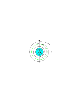
Figure 1: Phase Portrait for the noiseless system of (5.34).

Applying Proposition 4.1 and Theorem 3.1, we obtain that

$$\mu^{\varepsilon}\xlongrightarrow{w}\frac{1}{2\pi}\int_{0}^{2\pi}\delta_{\Psi_{t}\big{(}(2,0)\big{)}}(\cdot)dt\ {\rm as}\ \varepsilon\rightarrow 0.$$

Suppose that $C^{2}$ function $f$ in (5.34) is replaced by

$$f(s)\begin{cases}<0,\quad&s\in[0,1),\\ \equiv 0,\quad&s\in[1,4],\\ <0,\quad&s>4.\end{cases}$$

Then it follows from Proposition 5.4 that the annulus region $D_{1}:=\{(x_{1},x_{2}):1\leq r\leq 2\}$ is is an equivalent class, which is asymptotically orbitally stable from the exterior and asymptotically orbitally unstable from the interior. Besides, the origin $O$ is an attractor and $B(\Psi)=D_{1}\cup\{O\}$ (see Figure 2).

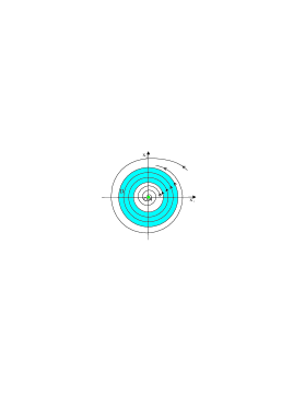
Figure 2: Phase Portrait for the noiseless system of (5.34).

Applying Proposition 4.1 and Theorem 3.2, we get that

$$\mu^{\varepsilon}\xlongrightarrow{w}\delta_{O}(\cdot)\ {\rm as}\ \varepsilon\rightarrow 0.$$

Example 5.6.

Consider two dimensional $C^{2}$ SDEs possessing infinite equivalent classes.

$$\left\{\begin{aligned} dx_{1}=&\Big{(}-x_{2}+x_{1}\big{(}1-x_{1}^{2}-x_{2}^{2}\big{)}^{5}\sin^{2}\big{(}1-x_{1}^{2}-x_{2}^{2}\big{)}^{-1}\Big{)}dt+\varepsilon\sigma_{1}(x_{1},x_{2})dw_{t}^{1}\\ dx_{2}=&\Big{(}x_{1}+x_{2}\big{(}1-x_{1}^{2}-x_{2}^{2}\big{)}^{5}\sin^{2}\big{(}1-x_{1}^{2}-x_{2}^{2}\big{)}^{-1}\Big{)}dt+\varepsilon\sigma_{2}(x_{1},x_{2})dw_{t}^{2}.\end{aligned}\right.$$ (5.35)

Proposition 5.7.

For (5.35), we have

$$\mu^{\varepsilon}\xlongrightarrow{w}\frac{1}{2\pi}\int_{0}^{2\pi}\delta_{\Psi_{t}\big{(}(1,0)\big{)}}(\cdot)dt\ {\rm as}\ \varepsilon\rightarrow 0.$$ (5.36)

The same result holds if the function $\big{(}1-x_{1}^{2}-x_{2}^{2}\big{)}^{5}\sin^{2}\big{(}1-x_{1}^{2}-x_{2}^{2}\big{)}^{-1}$ in (5.35) is replaced by a $C^{2}$ function $f$ with the following properties

$$f(s)=\begin{cases}f^{-}(s)\geq 0,\quad&s\in[0,1),\\ 0,\quad&s=1,\\ f^{+}(s)\leq 0,\quad&s>1\end{cases}$$

where

$$f^{-}(s)\begin{cases}\equiv 0,\quad&s\in I:=\bigcup_{n=1}^{\infty}[1-\frac{1}{(2n-1)\pi},1-\frac{1}{2n\pi}],\\ >0,\quad&s\in[0,1)\backslash I;\end{cases}$$

and

$$f^{+}(s)\begin{cases}\equiv 0,\quad&s\in J:=\bigcup_{n=1}^{\infty}[1+\frac{1}{2n\pi},1+\frac{1}{(2n-1)\pi}],\\ <0,\quad&(1,+\infty)\backslash J.\end{cases}$$

Proof.

Global dynamics of the corresponding determined system of (5.35) is analyzed as follows. The origin $O(0,0)$ is a repeller. The unit circle $S$ is a closed orbit, which is accumulated by a series of semistable limit cycles:

$$\Gamma_{n}:r=\sqrt{1-\frac{1}{n\pi}},\ n=\pm 1,\pm 2,\pm 3,\cdots.$$

The Birkhoff center $B(\Psi)=\{O\}\bigcup_{n=-\infty}^{n=+\infty}\Gamma_{n}$ with $\Gamma_{0}=S$. The global phase portraits are sketched in Figure 3.

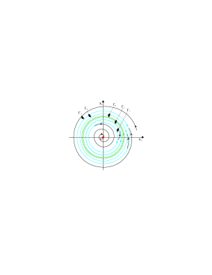
Figure 3: Phase Portrait for the noiseless system of (5.35).

Theorem 3.1 applies to the repeller origin, we know that there is no concentration on the origin $O$. Let $R_{n}$ denote the annulus surrounded by $\Gamma_{n}$ and $\Gamma_{-n}$ for any positive integer $n$. Then $R_{n}$ is an attractor. Utilizing Theorem 3.2 to semistable limit cycles $\{\Gamma_{m}:\ m=\pm 1,\pm 2,\pm 3,\cdots,\pm(n-1)\}$ and the attractor $R_{n}$, we conclude that there is no concentration on semistable limit cycles $\{\Gamma_{m}:\ m=\pm 1,\pm 2,\pm 3,\cdots,\pm(n-1)\}$. Since $n$ is arbitrary, we get (5.36).

Moreover, let the $C^{2}$ function $f$ satisfies the given properties and define the annuli

$$\mathcal{A}_{-n}:=\left\{\sqrt{1-\big{(}(2n-1)\pi\big{)}^{-1}}\leq r\leq\sqrt{1-\big{(}2n\pi\big{)}^{-1}}\right\},$$

$$\mathcal{A}_{n}:=\left\{\sqrt{1+\big{(}2n\pi\big{)}^{-1}}\leq r\leq\sqrt{1+\big{(}(2n-1)\pi\big{)}^{-1}}\right\},\ {\rm and}$$

$$\mathcal{R}_{n}:=\left\{\sqrt{1-\big{(}(2n-1)\pi\big{)}^{-1}}\leq r\leq\sqrt{1+\big{(}(2n-1)\pi\big{)}^{-1}}\right\}$$

for $n=1,2,\cdots$. It follows that $B(\Psi)=\{O\}\bigcup_{n=-\infty}^{n=+\infty}\mathcal{A}_{n}$ with $\mathcal{A}_{0}=S$. The global phase portraits are sketched in Figure 4.

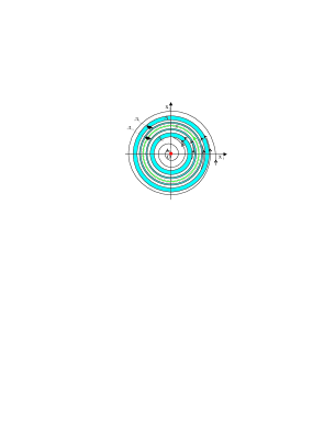
Figure 4: Phase Portrait for the noiseless system of (5.35).

Then by Proposition 5.4, $\mathcal{A}_{-n}$ and $\mathcal{A}_{n}$ are equivalent classes for each $n$. Replacing by $\Gamma_{n}$, $\Gamma_{-n}$ and $R_{n}$ by $\mathcal{A}_{n}$, $\mathcal{A}_{-n}$ and $\mathcal{R}_{n}$, respectively, we obtain (5.36) in the same manner. ∎

Example 5.8.

Let $H(x_{1},x_{2}):=\frac{x_{2}^{2}}{2}+\frac{x_{1}^{4}}{4}-\frac{x_{1}^{2}}{2}\in[-\frac{1}{4},+\infty)$. Consider two dimensional nondegenerate SDEs:

$$dx=[\mathcal{H}(H)-F(H)\nabla H]dt+\varepsilon\sigma(x)dw_{t}$$ (5.37)

where $C^{1}$ function $F$ is taken

$$F_{i}(s)=\begin{cases}(-1)^{i}|s|^{3},\quad&s\in[-\frac{1}{4},0),\\ s^{5}\sin^{2}\frac{\pi}{s},\quad&s\in[0,1],\\ >0,\quad&s\in(1,2),\\ 1,\quad&s\in[2,+\infty),\\ \end{cases}$$

for $i=1,2$, or

$$F_{j}(s)=\begin{cases}(-1)^{j}|s|^{3},\quad&s\in[-\frac{1}{4},0),\\ G(s),\\ \end{cases}$$

for $j=3,4$. Here $G:[0,+\infty)\rightarrow[0,1]$ is a $C^{\infty}$ function satisfying that $G(0)=0$ and there exist a sequence of intervals $I_{n}=[a_{n},b_{n}]\subset(0,1),n=1,2,3,\cdots$ with $I_{n+1}\subset I_{n}$, $\lim_{n\rightarrow\infty}b_{n}=0$ and $b_{1}=1$ such that $G(s)=0$ for any $s\in I=\bigcup_{n=1}^{\infty}I_{n}$ and $G(s)>0$ for any $s\in(0,+\infty)\backslash I$. Note that such a $G$ can be constructed by cut-off functions.

For these systems, we have the following conclusions.

Proposition 5.9.

For $i=1,3$, we have

$$\mu^{\varepsilon}\xlongrightarrow{w}\delta_{O}(\cdot)\ {\rm as}\ \varepsilon\rightarrow 0;$$ (5.38)

and for $i=2,4$, we have

$$\mu^{\varepsilon}\xlongrightarrow{w}\lambda_{1}\delta_{(1,0)}(\cdot)+\lambda_{2}\delta_{(-1,0)}(\cdot)\ {\rm as}\ \varepsilon\rightarrow 0$$ (5.39)

with $\lambda_{1}+\lambda_{2}=1$.

Proof.

For $i=1$, by definition of solution, $H^{-1}\big{(}n^{-1}\big{)}$ is a limit cycle of (5.31) for $n=1,2,3,\cdots$, which is asymptotically orbitally stable from the exterior and asymptotically orbitally unstable from the interior. These limit cycles accumulate on the homoclinic cycle, a figure-eight curve. Using $H$ as a Liapunov function, we can prove that any limit set of $\Psi$ lies on the zero set of $F(H)|\nabla H|^{2}$ (see Figure 5).

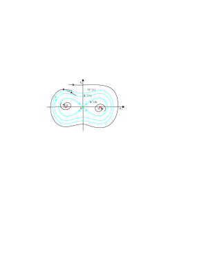
Figure 5: Phase Portrait for the noiseless system of (5.37) as $i=1$.

Thus $B(\Psi)=\bigcup_{n=1}^{+\infty}H^{-1}\big{(}n^{-1}\big{)}\bigcup H^{-1}(0)\bigcup\{(\pm 1,0)\}$.

Let $\mu^{\varepsilon}_{k}\xlongrightarrow{w}\mu$ as $\varepsilon_{k}\rightarrow 0$. Using $H+\frac{1}{4}$ as a Liapunov function, we can verify that $(\pm 1,0)$ is a repeller. Theorem 3.1 implies that there is no concentration of $\mu$ on the equilibria $(\pm 1,0)$. Again using the Liapunov method, we can prove that $H^{-1}\big{(}[-4^{-1},n^{-1}]\big{)}$ is an attractor for each $n$. Utilizing Theorem 3.2 to semistable limit cycles $\{H^{-1}\big{(}m^{-1}\big{)}:\ m=1,2,3,\cdots,n-1\}$ and the attractor $H^{-1}\big{(}[-4^{-1},n^{-1}]\big{)}$, we conclude that there is no concentration of $\mu$ on semistable limit cycles $\{H^{-1}\big{(}m^{-1}\big{)}:\ m=1,2,3,\cdots,n-1\}$. Since $n$ is arbitrary, we obtain that ${\rm supp}(\mu)\subset H^{-1}(0)$. Since $H^{-1}(0)$ consists of two homoclinic orbits connecting the origin $O$, it follows from the invariance of $\mu$ with respect to $\Psi$ that $\mu$ must be $\delta_{O}(\cdot)$. This proves (5.38).

For $i=3$, the annular region $H^{-1}\big{(}[a_{n},b_{n}]\big{)}$ is full of nontrivial periodic orbits of (5.31) for $n=1,2,3,\cdots$, which is asymptotically orbitally stable from the exterior and asymptotically orbitally unstable from the interior. These annular regions accumulate on the homoclinic cycle. Similarly, $B(\Psi)=\bigcup_{n=1}^{+\infty}H^{-1}\big{(}[a_{n},b_{n}]\big{)}\bigcup H^{-1}(0)\bigcup\{(\pm 1,0)\}$.

Let $\mu^{\varepsilon}_{k}\xlongrightarrow{w}\mu$ as $\varepsilon_{k}\rightarrow 0$. In the same manner we can prove that there is no concentration of $\mu$ on the equilibria $(\pm 1,0)$ and that $H^{-1}\big{(}[-4^{-1},b_{n}]\big{)}$ is an attractor for each $n$. By Proposition 5.4, the annular region $H^{-1}\big{(}[a_{n},b_{n}]\big{)}$ is an equivalent class for each $n$. Applying Theorem 3.2 to the annular regions $\{H^{-1}\big{(}[a_{m},b_{m}]\big{)}:\ m=1,2,3,\cdots,n-1\}$ and the attractor $H^{-1}\big{(}[-4^{-1},b_{n}]\big{)}$, we conclude that there is no concentration of $\mu$ on the annular regions $\{H^{-1}\big{(}[a_{m},b_{m}]\big{)}:\ m=1,2,3,\cdots,n-1\}$. Since $n$ is arbitrary, we obtain that ${\rm supp}(\mu)\subset H^{-1}(0)$ and (5.38) holds.

Suppose that $i=2,4$. Then the same procedure proves that there is no concentration of $\mu$ on both $H^{-1}\big{(}n^{-1}\big{)}$ and $H^{-1}\big{(}[a_{n},b_{n}]\big{)}$ for each $n$. Again using $H+\frac{1}{4}$ as a Liapunov function, we can verify that $(\pm 1,0)$ are attractors for both cases. Since every trajectory of $\Psi$ in the interior of $H^{-1}(0)$ other than $(\pm 1,0)$ converges to $H^{-1}(0)$ as $t\rightarrow-\infty$ and to $(\pm 1,0)$ as $t\rightarrow+\infty$ (see Figure 6).

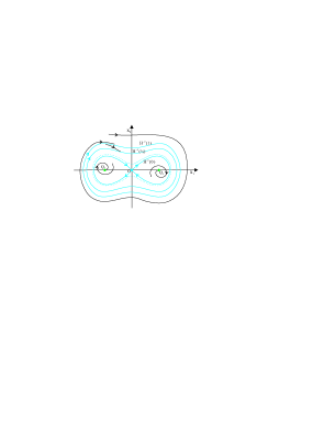
Figure 6: Phase Portrait for the noiseless system of (5.37) as $i=2$.

Applying Theorem 3.2 to $H^{-1}(0)$ and $(\pm 1,0)$, we get that $\mu\big{(}H^{-1}(0)\big{)}=0$. Finally, ${\rm supp}(\mu)=\{(\pm 1,0)\}$, which proves (5.39). ∎

Examples 5.6 and 5.8 show that there is no concentration on semistable limit cycles. Actually, this result holds for any planar systems by Theorem3.2. However, the following two examples illustrates limit measure can be supported on saddle-node (semistable equilibrium). The essential reason is that there is a cycle connecting it.

Example 5.10.

Consider two dimensional SDEs:

$$\left\{\begin{aligned} dx_{1}=&\big{[}x_{1}(1-x_{1}^{2}-x_{2}^{2})-x_{2}(1+x_{1})\big{]}dt+\varepsilon\sigma_{1}(x_{1},x_{2})dw_{t}^{1}\\ dx_{2}=&\big{[}x_{1}(1+x_{1})+x_{2}(1-x_{1}^{2}-x_{2}^{2})\big{]}dt+\varepsilon\sigma_{2}(x_{1},x_{2})dw_{t}^{2}.\end{aligned}\right.$$ (5.40)

The unperturbed system has equilibria $O(0,0)$ and $Q(-1,0)$, which make up the Birkhoff center $B(\Psi)$. $O$ is a repeller and $Q$ is a saddle-node which is connected by a homoclinic orbit on the unit circle, see Figure 7.

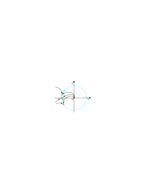
Figure 7: Phase Portrait for the noiseless system of (5.40).

By Theorem 3.1, there is no concentration on the origin $O$. Thus

$$\mu^{\varepsilon}\xlongrightarrow{w}\delta_{Q}(\cdot)\ {\rm as}\ \varepsilon\rightarrow 0.$$

Example 5.11.

Consider two dimensional SDEs:

$$\left\{\begin{aligned} dx_{1}=&\big{[}x_{1}\big{(}x_{1}^{2}+x_{2}^{2}\big{)}\big{(}1-x_{1}^{2}-x_{2}^{2}\big{)}-2x_{2}^{3}\big{]}dt+\varepsilon\sigma_{1}(x_{1},x_{2})dw_{t}^{1}\\ dx_{2}=&\big{[}x_{2}\big{(}x_{1}^{2}+x_{2}^{2}\big{)}\big{(}1-x_{1}^{2}-x_{2}^{2}\big{)}+2x_{1}x_{2}^{2}\big{]}dt+\varepsilon\sigma_{2}(x_{1},x_{2})dw_{t}^{2}.\end{aligned}\right.$$ (5.41)

The corresponding determined system has equilibria $O(0,0)$ and $(\pm 1,0)$, which comprise the Birkhoff center $B(\Psi)$. $O$ is a repeller and $(\pm 1,0)$ are saddle-nodes which are connected by two entire orbits on the unit circle, see Figure 8.

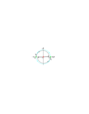
Figure 8: Phase Portrait for the noiseless system of (5.41).

By Theorem 3.1, there is no concentration on the origin $O$. Thus (5.39) holds.

Example 5.12.

Consider two dimensional determined system:

$$\left\{\begin{aligned} \frac{dx_{1}}{dt}=&x_{1}\left(x_{1}^{2}+x_{2}^{2}\right)\left(1-x_{1}^{2}-x_{2}^{2}\right)-x_{1}x_{2}\left(\sqrt{x_{1}^{2}+x_{2}^{2}}-x_{1}\right)\\ \frac{dx_{2}}{dt}=&x_{2}\left(x_{1}^{2}+x_{2}^{2}\right)\left(1-x_{1}^{2}-x_{2}^{2}\right)+x_{1}^{2}\left(\sqrt{x_{1}^{2}+x_{2}^{2}}-x_{1}\right).\end{aligned}\right.$$ (5.42)

The system (5.42) has equilibria $A(1,0)$, $B(0,1)$, $C(0,-1)$ and $O(0,0)$, $B$ is a stable node, $C$ is a saddle, $A$ is a saddle-node and $O$ is a repeller, $S^{1}$ is invariant and attracts all points except the origin $O$, see Figure 9.

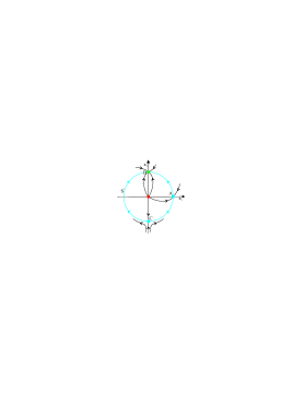
Figure 9: Phase Portrait for the system (5.42).

When the flow is restricted on $S^{1}$, it is topologically equivalent to that given by Kifer [22, Remark 5.4, p.90-91]. However, he chose a perturbation such that its limit measure is supported at the saddle-node $A$. But when (5.42) is perturbed by any nondegenerate while noise, its limit measure will sit on the stable node $B$ by Theorems 3.1 and 3.2, which is different from Kifer’s.

Example 5.13.

Consider the stochastic perturbation of the variational equation of the forced van der Pol oscillator:

$$\left\{\begin{aligned} du=&\big{[}u-\sigma v-u\big{(}u^{2}+v^{2}\big{)}\big{]}dt+\varepsilon\sigma_{1}(u,v)dw_{t}^{1}\\ dv=&\big{[}\sigma u+v-v\big{(}u^{2}+v^{2}\big{)}-\gamma\big{]}dt+\varepsilon\sigma_{2}(u,v)dw_{t}^{2}.\end{aligned}\right.$$ (5.43)

The corresponding determined system of (5.43) is the well-known variational equation of the forced van der Pol oscillator. In a neighborhood of the parameters $(\sigma,\gamma)=(\frac{1}{2},\frac{1}{2})$, Guchenheimer and Holmes [13, p.70-74] completely summarized the saddle-node bifurcations and Hopf bifurcations and drew $23$ phase portrait diagrams of the corresponding determined system in Figure 2.1.3 of [13, p.72].

Combing Theorems 3.1 and 3.2 with Figure 2.1.3 of [13, p.72], we conclude the following.

Proposition 5.14.

(i) There are $8$ diagrams having sources on which there is no concentration by Theorem 3.1;

(ii) there are $7$ diagrams having saddles on which there is no concentration by Theorem 3.2 (because there exist entire orbits connecting them to sinks or stable limit cycles);

(iii) there are $5$ diagrams having saddle-nodes on which there is no concentration by Theorem 3.2 (because there exist entire orbits connecting them to sinks or stable limit cycles);

(iv) there is one diagram having a codimension $2$ equilibrium on which there is no concentration by Theorem 3.2 (because there exists a entire orbit connecting it to a sink);

(v) there are $2$ diagrams having degenerate equilibria with a homoclinic orbit, which were sketched in the second line from bottom of [13, Figure 2.1.3, p.72], limit measure may be supported on them as in the Example 5.11.

Example 5.15.

Consider three dimensional SDEs:

$$dX^{\varepsilon}_{t}=b(X^{\varepsilon}_{t})dt+\varepsilon\sigma(X^{\varepsilon}_{t})dw_{t}$$ (5.44)

where $\sigma(X)$ is nondegenerate, $\sigma(-X)=\sigma(X)$ and $b(-X)=-b(X)$ for any $X\in\mathbb{R}^{3}$, $b(X)=b(x_{1},x_{2},x_{3})$ is a cooperative and irreducible vector field given by

$$\dot{X}=b(x_{1},x_{2},x_{3})=\left(-x_{1}+\frac{x_{3}}{1+|x_{3}|},x_{1}-x_{2},x_{2}-\frac{1}{2}x_{3}\right)^{*}.$$ (5.45)

The equilibria set of (5.45) is $O(0,0,0)$, $P_{\pm}=\pm(1,1,1)$, $O$ is a saddle and $P_{\pm}$ are asymptotically stable. There is a connecting orbit from $O$ to $P_{+}(P_{-})$. It follows from [34] that every trajectory of (5.45) tends to an equilibrium, see Figure 10.

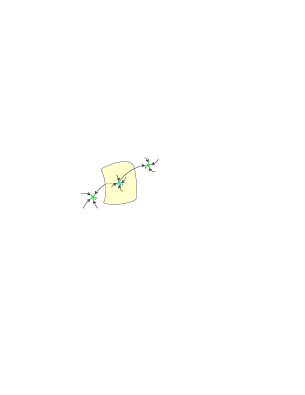
Figure 10: Phase Portrait for the vector field (5.45).

By symmetry of $b,\sigma$, the normalized solution $p^{\varepsilon}$ of the Fokker–Planck equation corresponding to (5.44) satisfies $p^{\varepsilon}(-X)=p^{\varepsilon}(X)$ for any $X\in\mathbb{R}^{3}$. Suppose that $\mu^{\varepsilon}$ is the stationary measure of (5.44). Then $p^{\varepsilon}$ is its density function. Let $\mu^{\varepsilon}\xlongrightarrow{w}\mu$ as $\varepsilon\rightarrow 0$. Then by Theorem 3.2, $\mu(O)=0$. It follows from the symmetry of $p^{\varepsilon}$ that as $\varepsilon\rightarrow 0$,

$$\mu^{\varepsilon}\xlongrightarrow{w}\frac{1}{2}\delta_{P_{-}}+\frac{1}{2}\delta_{P_{+}}.$$

Example 5.16.

Let $H=\frac{x_{1}^{4}}{4}-\frac{x_{1}^{2}}{2}+\frac{x_{2}^{2}}{2}$, $\mathcal{H}(H)=(x_{2},-(x_{1}^{3}-x_{1}))^{*}$, $\nabla H=((x_{1}^{3}-x_{1}),x_{2})^{*}$ and $b(X)=\mathcal{H}(H)-(H+\frac{1}{8})\nabla H$. Consider two dimensional SDEs:

$$dX^{\varepsilon}_{t}=b(X^{\varepsilon}_{t})dt+\varepsilon\sigma(X^{\varepsilon}_{t})dw_{t}$$ (5.46)

where $\sigma(X)$ is nondegenerate, $\sigma(-X)=\sigma(X)$ for any $X\in\mathbb{R}^{2}$. It is easy to see $b(-X)=-b(X)$ for any $X\in\mathbb{R}^{2}$. The corresponding perturbed system of (5.46) is

$$\dot{X}=b(X).$$ (5.47)

The equilibria set of (5.47) is $O(0,0)$, $P_{\pm}=(\pm 1,0)$, $O$ is a saddle without any homoclinic orbit and $P_{\pm}$ are repellers. Besides, $H+\frac{1}{8}=0$ consists of two limit cycles $\Gamma_{+}$ and $\Gamma_{-}$, which are attractors, $B(\Psi)=\Gamma_{\pm}\cup\{O,P_{\pm}\}$, see Figure 11.

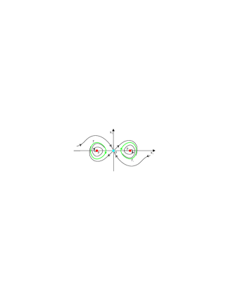
Figure 11: Phase Portrait for the noiseless system of (5.46).

By symmetry of $b,\sigma$, the normalized solution $p^{\varepsilon}$ of the Fokker–Planck equation corresponding to (5.46) satisfies $p^{\varepsilon}(-X)=p^{\varepsilon}(X)$ for any $X\in\mathbb{R}^{2}$. Suppose that $\mu^{\varepsilon}$ is the stationary measure of (5.46). Then $p^{\varepsilon}$ is its density function. Let $\mu^{\varepsilon}\xlongrightarrow{w}\mu$ as $\varepsilon\rightarrow 0$. Then by Theorems 3.1 and 3.2, $\mu(P_{\pm})=\mu(O)=0$. It follows from the symmetry of $p^{\varepsilon}$ that

$$\mu^{\varepsilon}\xlongrightarrow{w}\frac{1}{2}\left\{\frac{1}{T}\int_{0}^{T}\delta_{\Psi_{t}\big{(}(\sqrt{2},0)\big{)}}(\cdot)dt+\frac{1}{T}\int_{0}^{T}\delta_{\Psi_{t}\big{(}(-\sqrt{2},0)\big{)}}(\cdot)dt\right\}\ {\rm as}\ \varepsilon\rightarrow 0.$$

The last example shows that Theorem 3.1 is not valid if ${\bf\big{(}P_{\mathcal{R}}\big{)}}$ is violated.

Example 5.17.

Consider stochastic differential equations

$$\left\{\begin{array}[]{ll}\mathrm{d}x=[y-x(x^{2}+y^{2}-1)(x^{2}+y^{2}-2)]\mathrm{d}t+\varepsilon\mathrm{d}w^{1}_{t},\\ \mathrm{d}y=[-x-y(x^{2}+y^{2}-1)(x^{2}+y^{2}-2)]\mathrm{d}t+\varepsilon\mathrm{d}w^{2}_{t}.\end{array}\right.$$ (5.48)

The phase portrait for the unperturbed system are shown in Figure 12 below.

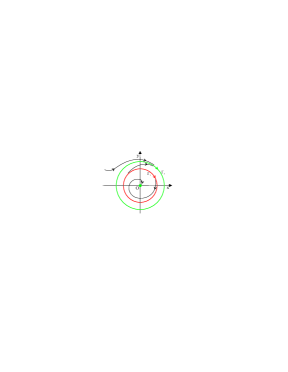
Figure 12: Phase Portrait for the noiseless system of (5.48).

Here $O=(0,0)$ is a stable focus, $\Gamma_{1}=\{(x,y)\in\mathbb{R}^{2}:x^{2}+y^{2}=1\}$ is an unstable limit cycle and $\Gamma_{2}=\{(x,y)\in\mathbb{R}^{2}:x^{2}+y^{2}=2\}$ is a stable limit cycle. Set $\mathcal{R}=\{(x,y)\in\mathbb{R}^{2}:x^{2}+y^{2}\leq 1\}$. Then $\mathcal{R}$ is a repeller for the unperturbed system. Using the method in [3], we can verify that the unique invariant probability density for (5.48) is

$$p^{\varepsilon}(x,y)=C(\varepsilon)\exp\big{(}-2\varepsilon^{-2}U(x,y)\big{)},$$

where $U(x,y)=(x^{2}+y^{2})^{3}/6-3(x^{2}+y^{2})^{2}/4+x^{2}+y^{2}$ and $C(\varepsilon)=\left(\int_{\mathbb{R}^{2}}\exp\big{(}-2\varepsilon^{-2}U(x,y)\big{)}\mathrm{d}x\mathrm{d}y\right)^{-1}<+\infty$. Since $U(O)=0<\frac{1}{3}=U(x,y)$ for $(x,y)\in\Gamma_{2}$, by Laplace’s method, $\mu^{\varepsilon}\xlongrightarrow{w}\delta_{O}$ as $\varepsilon\rightarrow 0$. This implies that the limit measure is concentrated on the repeller $\mathcal{R}$.

6 Appendix

In this section, we first prove Proposition 2.3 under ${\bf(0_{w})}$ and dissipativity condition of (1.2). The central objective of this appendix is to prove Theorem 3.1 and Theorem 4.3 under FWULDP. The next proposition can be deduced easily from the compactness assumption in ${\bf(0_{w})}$.

Proposition 6.1.

Let ${\bf(0_{w})}$ hold. If $F\subset{\bf C}_{T}$ is closed with $\cup_{t\in[0,T]}F^{t}:=\cup_{t\in[0,T]}\{\varphi(t):\varphi\in F\}$ being bounded, then there is a $\psi\in F$ such that

$$S_{T}(\psi)=\inf_{\varphi\in F}S_{T}(\varphi)=:S_{T}(F).$$

Proposition 6.2.

Suppose that (1.2) is dissipative. Then for any bounded set $A$, there is a positively invariant compact set $K\supset A$.

Proof.

Since $\Psi$ is dissipative, it has a global attractor $\mathcal{A}$ whose basin is $\mathbb{R}^{r}$. Then it follows from Wilson [41, Theorem 3.2] that $\mathcal{A}$ has a $C^{\infty}$ Liapunov function $V:\mathbb{R}^{r}\rightarrow\mathbb{R}_{+}$ satisfying

$$V(\mathcal{A})=0,\ V(x)\wedge\langle-b(x),\nabla V(x)\rangle>0,\ x\in\mathbb{R}^{r}\setminus\mathcal{A},\ {\rm and}\lim_{|x|\rightarrow+\infty}V(x)=+\infty.$$

For any $\delta>0$, $V^{-1}([0,\delta])$ is a positively invariant compact set. By the compactness of $\overline{A}$ and $\lim_{|x|\rightarrow+\infty}V(x)=+\infty$, there exists an integer $m$ such that $\overline{A}\subset V^{-1}([0,m])=:K$, which is positively invariant and compact. ∎

Proof of Proposition 2.3. We shall prove the proposition by contradiction. Suppose that $\{\varphi_{n}\}$ is a sequence of functions in $F$ satisfying $\lim_{n\rightarrow\infty}S_{T}(\varphi_{n})=0$. Then by Proposition 6.2 we may choose a positively invariant compact set $K_{1}:=V^{-1}([0,m])\supset F^{0}$. According to the proof of Proposition 6.2, $K_{2}:=V^{-1}([0,(m+1)])$ satisfies ${\rm Int}K_{2}\supset K_{1}$. Now for every $\varphi_{n}$, define $\phi_{n}$ to be $\varphi_{n}$ if $\varphi_{n}([0,T])\subset{\rm Int}K_{2}$. Otherwise, set $T_{*}^{n}=T_{*}(\varphi_{n}):=\inf\{t\in[0,T]:\varphi_{n}(t)\in\partial K_{2}\}$. Let $\phi_{n}$ be the same as $\varphi_{n}$ for $t\in[0,T_{*}^{n}]$ and extend it by the solution of system (1.2) for $t\in[T_{*}^{n},T]$. We emphasize that in the second case, $\phi_{n}$ can not be a solution of system (1.2) since $K_{1}$ is positively invariant with respect to $\Psi$ and $\phi_{n}(0)=\varphi_{n}(0)\in K_{1}$. We also have $\phi_{n}([0,T])\subset K_{2}$ and $\lim_{n\rightarrow\infty}S_{T}(\phi_{n})=0$. This means that after dropping finite terms, we may assume $\{\phi_{n}\}\subset\{\varphi\in{\bf C}_{T}:\varphi(t)\in K_{2},t\in[0,T],S_{T}(\varphi)\leq 1\}=:\mathcal{F}$. Recall that $\mathcal{F}$ is compact in $\mathbf{C}_{T}$ by ${(\bf 0_{w})}$. So we may assume again there is a $\phi_{*}\in\mathcal{F}$ such that $\lim_{n\rightarrow\infty}\phi_{n}=\phi_{*}$ with $\phi_{*}(0)\in K_{1}$. Indeed, $\phi_{*}$ can not be a solution of system (1.2). Otherwise for sufficiently large $n$, we have $\phi_{n}$ close enough to $\phi_{*}$ so that $\phi_{n}([0,T])\subset{\rm Int}K_{2}$. However, from the construction of $\phi_{n}$ we know that this means $\phi_{n}=\varphi_{n}$. As a result, $\phi_{*}\in F$ by the closedness of $F$, which contradicts the hypothesis of this proposition. Finally, from the lower semi-continuity of $S_{T}$ and Remark 1, we conclude that $\liminf_{n\rightarrow\infty}S_{T}(\phi_{n})\geq S_{T}(\phi_{*})>0$, a contradiction.

We now proceed to prove Theorem 3.1 under FWULDP.

Proof of Theorem 3.1 Under FWULDP. Choose $\delta>0$ such that $(\mathcal{R})_{\delta}$ is a fundamental neighborhood of $\mathcal{R}$. By Lemma 4.1, there exists $\delta_{1},\ \delta^{*}_{2}\in(0,\delta),\ \delta_{1}>\delta^{*}_{2}$ and $s_{0}>0$ such that $V(\partial(\mathcal{R})_{\delta_{1}},\partial(\mathcal{R})_{\delta^{*}_{2}})\geq s_{0}$. Set $\delta_{2}=\delta^{*}_{2}/2$. Applying Proposition 2.1 to $(\mathcal{R})_{\delta}$ and $\overline{(\mathcal{R})_{\delta_{1}}}\backslash(\mathcal{R})_{\delta_{2}}$, we have $T_{0}=\inf\big{\{}u\geq 0:\Psi_{t}\big{(}\overline{(\mathcal{R})_{\delta_{1}}}\backslash(\mathcal{R})_{\delta_{2}}\big{)}\subset((\mathcal{R})_{\delta})^{c},t\geq u\big{\}}<+\infty$. Let $F_{0}=\{\varphi\in{\bf C}_{T_{0}}:\varphi(0)\in\overline{(\mathcal{R})_{\delta_{1}}}\backslash(\mathcal{R})_{\delta_{2}},\varphi(T_{0})\in\overline{(\mathcal{R})_{\delta_{1}}}\}$ be a closed subset of ${\bf C}_{T_{0}}$. Then $F_{0}^{0}$ is bounded and $F_{0}$ does not contain any solution of system (1.2) by the definition of $T_{0}$. Then by Hypothesis 2.2, we have $s_{1}=S_{T_{0}}(F_{0})>0$.

We now follow the line of proof for Theorem 3.1 under DZULDP to prove the same result under FWULDP. The central tasks are to prove that (4.17), (4.18) and (4.19). The same procedure proves (4.20).

For any $y\in\partial(\mathcal{R})_{\delta_{1}}$, let $F_{1,y}=\{\varphi\in{\bf C}_{T}^{y}:\varphi(t)\in\partial(\mathcal{R})_{\delta_{2}}\>\textrm{for some}\ t\in[0,T]\}$ where $T$ is the same in the proof of Theorem 3.1 under DZULDP. For any $\tilde{\varphi}\in\{\varphi\in\mathbf{C}^{y}_{T}:\rho_{T}(\varphi,F_{1,y})<\delta^{*}_{2}-\delta_{2}\}$, there exists $\hat{\varphi}\in F_{1,y},\hat{t}\in[0,T]$ such that $\tilde{\varphi}(\hat{t})\in B(\hat{\varphi}(\hat{t}),\delta^{*}_{2}-\delta_{2})\subset(\mathcal{R})_{\delta^{*}_{2}}$. From the continuity of $\tilde{\varphi}$, we know that there is some $\tilde{t}=\tilde{t}(\tilde{\varphi})\in[0,T]$ such that $\tilde{\varphi}(\tilde{t})\in\partial(\mathcal{R})_{\delta^{*}_{2}}$. By the definition of $V(\partial(\mathcal{R})_{\delta_{1}},\partial(\mathcal{R})_{\delta^{*}_{2}})$ and Lemma 4.1, we have

$$\inf_{y\in\partial(\mathcal{R})_{\delta_{1}}}S_{T}^{y}\big{(}\{\varphi\in\mathbf{C}^{y}_{T}:\rho_{T}(\varphi,F_{1,y})<\delta^{*}_{2}-\delta_{2}\}\big{)}\geq V(\partial(\mathcal{R})_{\delta_{1}},\partial(\mathcal{R})_{\delta^{*}_{2}})\geq s_{0}.$$

This proves that

$$\mathbb{F}_{T}^{y}(0.9s_{0})\cap\{\varphi\in\mathbf{C}^{y}_{T}:\rho_{T}(\varphi,F_{1,y})<\delta^{*}_{2}-\delta_{2}\}=\emptyset$$

and

$$F_{1,y}\subset\{\varphi\in\mathbf{C}^{y}_{T}:\rho_{T}(\varphi,\mathbb{F}_{T}^{y}(0.9s_{0}))\geq\delta^{*}_{2}-\delta_{2}\}$$

which means that $\{X^{\varepsilon}\in F_{1,y}\}\subset\{X^{\varepsilon}(0)=y,\rho_{T}(X^{\varepsilon},\mathbb{F}_{T}^{y}(0.9s_{0}))\geq\delta^{*}_{2}-\delta_{2}\},\forall y\in\partial(\mathcal{R})_{\delta_{1}}.$ By (2.6) of ${\bf(II_{u})}$, there exists $\varepsilon_{1}>0$ such that for any $\varepsilon\in(0,\varepsilon_{1})$ and $y\in\partial(\mathcal{R})_{\delta_{1}}$, we get

$$\mathbb{P}_{y}(\tau\leq T)=\mathbb{P}_{y}(X^{\varepsilon}\in F_{1,y}) \leq\mathbb{P}_{y}\{\rho_{T}(X^{\varepsilon},\mathbb{F}_{T}^{y}(0.9s_{0}))\geq\delta^{*}_{2}-\delta_{2}\}$$

$$\leq\exp\{-\varepsilon^{-2}(0.9s_{0}-0.1s_{0})\}\leq\exp\{-0.8s_{0}/\varepsilon^{2}\}.$$ (6.49)

Therefore, by (4.20) and (6), for any $\varepsilon\in(0,\varepsilon_{1})$,

$$\sup_{z\in\big{(}\overline{(\mathcal{R})_{\delta_{1}}}\big{)}^{c}}\mathbb{P}_{z}(X^{\varepsilon}_{T}\in(\mathcal{R})_{\delta_{2}})\leq\sup_{y\in\partial(\mathcal{R})_{\delta_{1}}}\mathbb{P}_{y}(\tau\leq T)\leq\exp\{-0.8s_{0}/\varepsilon^{2}\}.$$

Thus, the inequality (4.17) follows.

For any $z\in\overline{(\mathcal{R})_{\delta_{1}}}\backslash(\mathcal{R})_{\delta_{2}}$, let $F_{2,z}=\big{\{}\varphi\in{\bf C}_{T}^{z}:\varphi(T)\in\overline{(\mathcal{R})_{\delta_{2}}}\big{\}}$. We claim that

$$S_{T}\big{(}\{\varphi\in\mathbf{C}^{z}_{T}:\rho_{T}(\varphi,F_{2,z})<\delta^{*}_{2}-\delta_{2}\}\big{)}\geq s_{0}\wedge s_{1}.$$ (6.50)

Indeed, let $\tilde{\varphi}$ be any element in $\{\varphi\in\mathbf{C}^{z}_{T}:\rho_{T}(\varphi,F_{2,z})<\delta^{*}_{2}-\delta_{2}\}$. Recall the definition of $F_{2,z}$, we conclude that $\tilde{\varphi}(T)\in\overline{(\mathcal{R})_{\delta^{*}_{2}}}$. If $S_{T}(\tilde{\varphi})<s_{1}$, then by the definition of $s_{1}$, we have $\tilde{\varphi}(T_{0})\notin\overline{(\mathcal{R})_{\delta_{1}}}$. Thanks to the continuity of $\tilde{\varphi}$ and $\tilde{\varphi}(T)\in\overline{(\mathcal{R})_{\delta^{*}_{2}}}$, there exist $t_{1},t_{2}\in(T_{0},T],t_{1}<t_{2}$ such that $\tilde{\varphi}(t_{1})\in\partial(\mathcal{R})_{\delta_{1}},\tilde{\varphi}(t_{2})\in\partial(\mathcal{R})_{\delta^{*}_{2}}$. Therefore, $S_{T}(\tilde{\varphi})\geq S_{t_{1}t_{2}}(\tilde{\varphi})\geq V(\partial(\mathcal{R})_{\delta_{1}},\partial(\mathcal{R})_{\delta^{*}_{2}})\geq s_{0}\geq s_{0}\wedge s_{1}$. This proves the claim. As a result, $\{X^{\varepsilon}\in F_{2,z}\}\subset\{X^{\varepsilon}(0)=z,\rho_{T}(X^{\varepsilon},\mathbb{F}_{T}^{z}(0.9(s_{0}\wedge s_{1})))\geq\delta^{*}_{2}-\delta_{2}\},\forall z\in\overline{(\mathcal{R})_{\delta_{1}}}\backslash(\mathcal{R})_{\delta_{2}}.$ By (2.6) of ${\bf(II_{u})}$, there exists $\varepsilon_{2}>0$ such that for any $\varepsilon\in(0,\varepsilon_{2})$ and $z\in\overline{(\mathcal{R})_{\delta_{1}}}\backslash(\mathcal{R})_{\delta_{2}}$, we have

$$\mathbb{P}_{z}(X^{\varepsilon}_{T}\in(\mathcal{R})_{\delta_{2}})\leq\mathbb{P}_{z}(X^{\varepsilon}\in F_{2,z})\leq\mathbb{P}_{z}\{\rho_{T}(X^{\varepsilon},\mathbb{F}_{T}^{z}(0.9(s_{0}\wedge s_{1})))\geq\delta^{*}_{2}-\delta_{2}\}\leq\exp\{-0.8(s_{0}\wedge s_{1})/\varepsilon^{2}\}.$$

Therefore the inequality (4.18) follows immediately.

The proof of (4.19) remains unchanged, as one may check below. Let $C=\{\varphi\in{\bf C}_{T}:\varphi(T)\notin(\mathcal{R})_{\delta_{2}}\},G=\{\varphi\in{\bf C}_{T}:\rho_{T}(\varphi,\psi^{x})<\delta_{*},x\in\overline{(\mathcal{R})_{\delta_{2}}}\}$, where $\delta_{*}=\delta-\delta_{2}$. Then $G$ is an open set in ${\bf C}_{T}$ and $G\subset C$ by (4.16). Furthermore, $\sup_{z\in\overline{(\mathcal{R})_{\delta_{2}}}}S_{T}^{z}(G)\leq\sup_{z\in\overline{(\mathcal{R})_{\delta_{2}}}}S_{T}(\psi^{z})\leq 0.1(s_{0}\wedge s_{1})$ by (4.15). By ${\bf(I_{u})}$, there exists $\varepsilon_{3}>0$ such that for any $\varepsilon\in(0,\varepsilon_{3})$ and $z\in\overline{(\mathcal{R})_{\delta_{2}}}$, we have

$$\mathbb{P}_{z}(X^{\varepsilon}_{T}\notin(\mathcal{R})_{\delta_{2}})= \mathbb{P}_{z}(X^{\varepsilon}\in C)$$

$$\geq \mathbb{P}_{z}(X^{\varepsilon}\in G)$$

$$\geq \exp\big{\{}-\big{(}\sup_{z\in\overline{(\mathcal{R})_{\delta_{2}}}}S_{T}(\psi^{z})+0.1(s_{0}\wedge s_{1})\big{)}/\varepsilon^{2}\big{\}}$$

$$\geq \exp\{-0.2(s_{0}\wedge s_{1})/\varepsilon^{2}\}.$$

where we have used ${\bf(I_{u})}$ in the second inequality $\geq$. From the above obtained inequality, we get that for any $\varepsilon\in(0,\varepsilon_{3})$ and $z\in\overline{(\mathcal{R})_{\delta_{2}}}$,

$$\mathbb{P}_{z}(X^{\varepsilon}_{T}\in(\mathcal{R})_{\delta_{2}})= 1-\mathbb{P}_{z}(X^{\varepsilon}_{T}\notin(\mathcal{R})_{\delta_{2}})$$

$$\leq 1-\exp\{-0.2(s_{0}\wedge s_{1})/\varepsilon^{2}\}.$$

So (4.19) follows easily from the above fact. This completes the proof.

Here is the proof of Theorem 4.3 with FWULDP.

Proof of Theorem 4.3 Under FWULDP. Let $\delta^{\prime}\in(0,{\rm dist}\left(y,\mathcal{A}\right)/2)$ such that $(\mathcal{A})_{\delta^{\prime}}$ is a fundamental neighborhood of $\mathcal{A}$. By Lemma 4.2, there exist $\delta_{1}>\delta^{*}_{1}>\delta_{2}>\delta_{3},\delta_{1},\delta^{*}_{1},\delta_{2},\delta_{3}\in(0,\delta^{\prime})$ and $s_{0}>0$ such that $V\left(\partial(\mathcal{A})_{\delta_{2}},\partial(\mathcal{A})_{\delta^{*}_{1}}\right)\geq s_{0}$. Since $\mathcal{A}$ is an attractor, we obtain $T_{0}:=\inf\big{\{}u\geq 0:\Psi_{t}\big{(}\overline{(\mathcal{A})_{\delta_{1}}}\big{)}\subset(\mathcal{A})_{\delta_{3}},t\geq u\big{\}}<+\infty$. The set $F_{0}=\{\varphi\in{\bf C}_{T_{0}}:\varphi(0)\in\overline{(\mathcal{A})_{\delta_{1}}},\varphi(T_{0})\in((\mathcal{A})_{\delta_{2}})^{c}\}$ is a closed subset of ${\bf C}_{T_{0}}$. $F_{0}^{0}$ is bounded and $F_{0}$ does not contain any solution of system (1.2). Thus, by Hypothesis 2.2, $s_{1}:=S_{T_{0}}(F_{0})>0$. Let $\delta=\delta_{2}\wedge\frac{s_{0}\wedge s_{1}}{10L}$, where $L=L_{\bar{B}_{\delta^{\prime}}(y)\cup\overline{(\mathcal{A})_{\delta^{\prime}}}}$ is a constant as Lemma 2.1. Since $V(y,\mathcal{A})=0$, there exist $T_{1}>0$ and $\tilde{\varphi}\in{\bf C}_{T_{1}}$ with $\tilde{\varphi}(0)=y$ and $\tilde{\varphi}(T_{1})\in\mathcal{A}$ such that $S_{T_{1}}(\tilde{\varphi})<0.2(s_{0}\wedge s_{1})$.

As in the proof of Theorem 4.3 Under DZULDP, we only have prove (4.27) and (4.28). Here we replace $0.9$ in (4.28) by $0.8$ and $\kappa$ in (4.23) by $0.4(s_{0}\wedge s_{1})$.

To prove (4.27), let $G^{z}=\{\varphi\in{\bf C}^{z}_{T}:\rho_{T}(\varphi,\psi^{z})<\delta_{1}\}$ for every $z\in\bar{B}_{\delta}(y)$. Fix $z\in\bar{B}_{\delta}(y)$. Recall $\psi^{z}(T)\in\mathcal{A}$, we get $\{X^{\varepsilon}_{0}=z,X^{\varepsilon}_{T}\in(\mathcal{A})_{\delta_{1}}\}\supset\{X^{\varepsilon}_{0}=z,X^{\varepsilon}\in G^{z}\}$. By ${\bf(I_{u})}$, there exists $\varepsilon_{1}>0$ such that for any $\varepsilon\in(0,\varepsilon_{1}),z\in\bar{B}_{\delta}(y)$ we have

$$\mathbb{P}_{z}\big{(}X^{\varepsilon}_{T}\in(\mathcal{A})_{\delta_{1}}\big{)}\geq\mathbb{P}_{z}\big{(}X^{\varepsilon}\in G^{z}\big{)}\geq\exp\big{\{}-\big{(}0.3(s_{0}\wedge s_{1})+0.1(s_{0}\wedge s_{1})\big{)}/\varepsilon^{2}\big{\}}=\exp\{-0.4(s_{0}\wedge s_{1})/\varepsilon^{2}\}.$$ (6.51)

Hence (4.27) follows from (6.51).

For any $z\in\overline{(\mathcal{A})_{\delta_{1}}}$, let $F_{z}=\{\varphi\in\mathbf{C}^{z}_{T}:\varphi(T)\notin(\mathcal{A})_{\delta_{1}}\}$. Next we show that $\inf_{z\in\overline{(\mathcal{A})_{\delta_{1}}}}S^{z}_{T}(\{\varphi\in\mathbf{C}^{z}_{T}:\rho_{T}(\varphi,F_{z})<\delta_{1}-\delta^{*}_{1}\})\geq s_{0}\wedge s_{1}$. In fact, fix $\tilde{z}\in\overline{(\mathcal{A})_{\delta_{1}}}$, let $\tilde{\varphi}\in\{\varphi\in\mathbf{C}^{\tilde{z}}_{T}:\rho_{T}(\varphi,F_{\tilde{z}})<\delta_{1}-\delta^{*}_{1}\}$. Because of the definition of $F_{\tilde{z}}$, we know that $\tilde{\varphi}(T)\notin(\mathcal{A})_{\delta^{*}_{1}}$. Either $S_{T}^{\tilde{z}}(\tilde{\varphi})\geq s_{1}$ or $S_{T}^{\tilde{z}}(\tilde{\varphi})<s_{1}$. Let us consider the later. Then $S_{T_{0}}^{\tilde{z}}(\tilde{\varphi})<s_{1}$. So $\tilde{\varphi}(T_{0})\in(\mathcal{A})_{\delta_{2}}$ from the definition of $s_{1}$. Note that $\tilde{\varphi}(T)\notin(\mathcal{A})_{\delta^{*}_{1}}$ and $\overline{(\mathcal{A})_{\delta_{2}}}\subset(\mathcal{A})_{\delta^{*}_{1}}$. Then by the continuity of $\tilde{\varphi}$, there exist $t_{1},t_{2}\in(T_{0},T],t_{1}>t_{2}$ such that $\tilde{\varphi}(t_{1})\in\partial(\mathcal{A})_{\delta^{*}_{1}},\tilde{\varphi}(t_{2})\in\partial(\mathcal{A})_{\delta_{2}}$. Thus $S_{T}^{\tilde{z}}(\tilde{\varphi})\geq S_{t_{2}t_{1}}^{\tilde{z}}(\tilde{\varphi})\geq V(\partial(\mathcal{A})_{\delta_{2}},\partial(\mathcal{A})_{\delta^{*}_{1}})\geq s_{0}$. Therefore $\inf_{z\in\overline{(\mathcal{A})_{\delta_{1}}}}S^{z}_{T}(\{\varphi\in\mathbf{C}^{z}_{T}:\rho_{T}(\varphi,F_{z})<\delta_{1}-\delta^{*}_{1}\})\geq s_{0}\wedge s_{1}$. As a result, $\{X^{\varepsilon}\in F_{z}\}\subset\{X^{\varepsilon}(0)=z,\rho_{T}(X^{\varepsilon},\mathbb{F}_{T}^{z}(0.9(s_{0}\wedge s_{1})))\geq\delta_{1}-\delta^{*}_{1}\},\forall z\in\overline{(\mathcal{A})_{\delta_{1}}}.$ Finally, by (2.6) of ${\bf(II_{u})}$, there exists $\varepsilon_{2}>0$ such that for any $\varepsilon\in(0,\varepsilon_{2}),z\in\overline{(\mathcal{A})_{\delta_{1}}}$ we have

$$\mathbb{P}_{z}\big{(}X^{\varepsilon}_{T}\notin(\mathcal{A})_{\delta_{1}}\big{)}=\mathbb{P}_{z}\big{(}X^{\varepsilon}\in F_{z}\big{)}\leq\mathbb{P}_{z}\{\rho_{T}(X^{\varepsilon},\mathbb{F}_{T}^{z}(0.9(s_{0}\wedge s_{1})))\geq\delta_{1}-\delta^{*}_{1}\}\leq\exp\{-0.8(s_{0}\wedge s_{1})/\varepsilon^{2}\}.$$

This implies

$$\int_{(\mathcal{A})_{\delta_{1}}}\mu^{\varepsilon}(dz)\mathbb{P}_{z}\big{(}X^{\varepsilon}_{T}\in(\mathcal{A})_{\delta_{1}}\big{)}= \int_{(\mathcal{A})_{\delta_{1}}}\mu^{\varepsilon}(dz)\big{(}1-\mathbb{P}_{z}\big{(}X^{\varepsilon}_{T}\notin(\mathcal{A})_{\delta_{1}}\big{)}\big{)}$$

$$= \mu^{\varepsilon}((\mathcal{A})_{\delta_{1}})-\int_{(\mathcal{A})_{\delta_{1}}}\mu^{\varepsilon}(dz)\mathbb{P}_{z}\big{(}X^{\varepsilon}_{T}\notin(\mathcal{A})_{\delta_{1}}\big{)}$$

$$\geq \mu^{\varepsilon}((\mathcal{A})_{\delta_{1}})-\mu^{\varepsilon}((\mathcal{A})_{\delta_{1}})\exp\{-0.8(s_{0}\wedge s_{1})/\varepsilon^{2}\}$$

for any $\varepsilon\in(0,\varepsilon_{2})$, i.e., the inequality (4.28) follows.

Acknowledgements This work is supported by the National Natural Science Foundation of China (Nos. 12171321, 12001373, 11771295, 11931004).

References

[1]
Michel Benaïm.
Recursive algorithms, urn processes and chaining number of chain
recurrent sets.
Ergodic Theory Dynam. Systems, 18(1):53–87, 1998.
[2]
Michel Benaïm and Morris W. Hirsch.
Dynamics of Morse-Smale urn processes.
Ergodic Theory Dynam. Systems, 15(6):1005–1030, 1995.
[3]
L. Chen, J. Jiang, and T. Xu.
On exact concentration of limit measures of quasipotential systems by
laplace’s method.
In Preprint, 2021.
[4]
Lifeng Chen, Zhao Dong, and Jifa Jiang.
A criterion on a repeller being a null set of any limit measure for
stochastic differential equations.
Sci. China Math., 64(2):221–238, 2021.
[5]
Lifeng Chen, Zhao Dong, and Jifa Jiang.
Stochastic stability of two-dimensional systems (in chinese).
Sci. Sin. Math., 51(11):1717–1730, 2021.
[6]
Lifeng Chen, Zhao Dong, Jifa Jiang, and Jianliang Zhai.
On limiting behavior of stationary measures for stochastic evolution
systems with small noise intensity.
Sci. China Math., 63(8):1463–1504, 2020.
[7]
Xinfu Chen, Carey Caginalp, Jianghao Hao, and Yajing Zhang.
Effects of white noise in multistable dynamics.
Discrete Contin. Dyn. Syst. Ser. B, 18(7):1805–1825, 2013.
[8]
Amir Dembo and Ofer Zeitouni.
Large Deviations Techniques and Applications, volume 38 of Stochastic Modelling and Applied Probability.
Springer-Verlag, Berlin, 2010.
Corrected reprint of the second (1998) edition.
[9]
Jin Feng and Thomas G. Kurtz.
Large Deviations for Stochastic Processes, volume 131 of Mathematical Surveys and Monographs.
American Mathematical Society, Providence, RI, 2006.
[10]
Lirui Feng, Yi Wang, and Jianhong Wu.
Generic behavior of flows strongly monotone with respect to high-rank
cones.
J. Differential Equations, 275:858–881, 2021.
[11]
Mark I. Freidlin and Alexander D. Wentzell.
Random Perturbations of Dynamical Systems, volume 260 of Grundlehren der mathematischen Wissenschaften [Fundamental Principles of
Mathematical Sciences].
Springer, Heidelberg, third edition, 2012.
Translated from the 1979 Russian original by Joseph Szücs.
[12]
Shaobo Gan and Lan Wen.
Nonsingular star flows satisfy Axiom A and the no-cycle
condition.
Invent. Math., 164(2):279–315, 2006.
[13]
John Guckenheimer and Philip Holmes.
Nonlinear Oscillations, Dynamical Systems, and Bifurcations of
Vector Fields, volume 42 of Applied Mathematical Sciences.
Springer-Verlag, New York, 1990.
Revised and corrected reprint of the 1983 original.
[14]
Philip Hartman.
Ordinary Differential Equations, volume 38 of Classics in
Applied Mathematics.
Society for Industrial and Applied Mathematics (SIAM), Philadelphia,
PA, 2002.
Corrected reprint of the second (1982) edition [Birkhäuser,
Boston, MA; MR0658490 (83e:34002)], With a foreword by Peter Bates.
[15]
Shuhei Hayashi.
Connecting invariant manifolds and the solution of the
stability and -stability conjectures for flows.
Ann. of Math. (2), 145(1):81–137, 1997.
[16]
Morris W. Hirsch.
Systems of differential equations that are competitive or
cooperative. IV. Structural stability in three-dimensional systems.
SIAM J. Math. Anal., 21(5):1225–1234, 1990.
[17]
Wen Huang, Min Ji, Zhenxin Liu, and Yingfei Yi.
Stochastic stability of measures in gradient systems.
Phys. D, 314:9–17, 2016.
[18]
Wen Huang, Min Ji, Zhenxin Liu, and Yingfei Yi.
Concentration and limit behaviors of stationary measures.
Phys. D, 369:1–17, 2018.
[19]
Chii-Ruey Hwang.
Laplace’s method revisited: weak convergence of probability measures.
Ann. Probab., 8(6):1177–1182, 1980.
[20]
Min Ji, Zhongwei Shen, and Yingfei Yi.
Quantitative concentration of stationary measures.
Phys. D, 399:73–85, 2019.
[21]
R. Z. Khasminskii.
The averaging principle for parabolic and elliptic differential
equations and Markov processes with small diffusion.
Teor. Verojatnost. i Primenen., 8:3–25, 1963.
[22]
Yuri Kifer.
Random Perturbations of Dynamical Systems, volume 16 of Progress in Probability and Statistics.
Birkhäuser Boston, Inc., Boston, MA, 1988.
[23]
Richard C. Kraaij, Frank Redig, and Rik Versendaal.
Classical large deviation theorems on complete Riemannian
manifolds.
Stochastic Process. Appl., 129(11):4294–4334, 2019.
[24]
John Mallet-Paret and George R. Sell.
The Poincaré-Bendixson theorem for monotone cyclic feedback
systems with delay.
J. Differential Equations, 125(2):441–489, 1996.
[25]
John Mallet-Paret and Hal L. Smith.
The Poincaré-Bendixson theorem for monotone cyclic feedback
systems.
J. Dynam. Differential Equations, 2(4):367–421, 1990.
[26]
J. Palis.
On Morse-Smale dynamical systems.
Topology, 8:385–404, 1968.
[27]
J. Palis and W. de Melo.
Geometric Theory of Dynamical Systems.
Springer-Verlag, New York-Berlin, 1982.
An introduction, Translated from the Portuguese by A. K. Manning.
[28]
J. Palis and S. Smale.
Structural stability theorems.
In Global Analysis (Proc. Sympos. Pure Math., Vol.
XIV, Berkeley, Calif., 1968), pages 223–231. Amer. Math. Soc.,
Providence, R.I., 1970.
[29]
Charles Pugh and Michael Shub.
The -stability theorem for flows.
Invent. Math., 11:150–158, 1970.
[30]
Clark Robinson.
Structural stability of vector fields.
Ann. of Math. (2), 99:154–175, 1974.
[31]
David Ruelle.
Small random perturbations of dynamical systems and the definition of
attractors.
Comm. Math. Phys., 82(1):137–151, 1981/82.
[32]
Michael Salins.
Equivalences and counterexamples between several definitions of the
uniform large deviations principle.
Probab. Surv., 16:99–142, 2019.
[33]
Luis A. Sanchez.
Cones of rank 2 and the Poincaré-Bendixson property for a new
class of monotone systems.
J. Differential Equations, 246(5):1978–1990, 2009.
[34]
James F. Selgrade.
Asymptotic behavior of solutions to single loop positive feedback
systems.
J. Differential Equations, 38(1):80–103, 1980.
[35]
Ya. G. Sinaĭ.
Kolmogorov’s work on ergodic theory.
Ann. Probab., 17(3):833–839, 1989.
[37]
Hal L. Smith.
Periodic orbits of competitive and cooperative systems.
J. Differential Equations, 65(3):361–373, 1986.
[38]
Jian Wang, Hao Yang, Jiangliang Zhai, and Tusheng Zhang.
Large deviation principles for sdes under locally weak monotonicity
conditions.
arXiv:2110.06444v1, 2021.
[39]
Lan Wen.
Differentiable Dynamical Systems, volume 173 of Graduate
Studies in Mathematics.
American Mathematical Society, Providence, RI, 2016.
An introduction to structural stability and hyperbolicity.
[40]
A. D. Wentzell and M. I. Freidlin.
Small random perturbations of dynamical systems.
Uspehi Mat. Nauk, 25(1 (151)):3–55, 1970.
[41]
F. Wesley Wilson, Jr.
Smoothing derivatives of functions and applications.
Trans. Amer. Math. Soc., 139:413–428, 1969.