Properties of the Non-Autonomous Lattice Sine-Gordon Equation

Properties of the Non-Autonomous
Lattice Sine-Gordon Equation:
Consistency around a Broken Cube Property

Nobutaka NAKAZONO

N. Nakazono

Institute of Engineering, Tokyo University of Agriculture and Technology,
2-24-16 Nakacho Koganei, Tokyo 184-8588, Japan nakazono@go.tuat.ac.jp https://researchmap.jp/nakazono/

Received February 03, 2022, in final form April 14, 2022; Published online April 20, 2022

The lattice sine-Gordon equation is an integrable partial difference equation on ${\mathbb{Z}}^{2}$, which approaches the sine-Gordon equation in a continuum limit. In this paper, we show that the non-autonomous lattice sine-Gordon equation has the consistency around a broken cube property as well as its autonomous version. Moreover, we construct two new Lax pairs of the non-autonomous case by using the consistency property.

lattice sine-Gordon equation; Lax pair; integrable systems; partial difference equations

37K10; 39A14; 39A45

1 Introduction

The sine-Gordon equation:

$$\phi_{tt}-\phi_{xx}+\sin{\phi}=0,$$ (1.1)

where $\phi=\phi(t,x)\in\mathbb{C}$ and $(t,x)\in\mathbb{C}^{2}$, is well known as a motion equation of a row of pendulums hang from a rod and are coupled by torsion springs. This equation is also known as a famous example of integrable systems. In 1992, the following autonomous difference equation was found [3, 20]:

$$\dfrac{u_{l+1,m+1}}{u_{l,m}}=\left(\dfrac{\gamma-u_{l+1,m}}{1-\gamma u_{l+1,m}}\right)\left(\dfrac{1-\gamma u_{l,m+1}}{\gamma-u_{l,m+1}}\right),$$ (1.2)

where $u_{l,m}\in\mathbb{C}$, $(l,m)\in\mathbb{Z}^{2}$ and $\gamma\in\mathbb{C}$, which is a discrete analogue of equation (1.1) and therefore called lattice sine-Gordon (lsG) equation. Note that it is not only equation (1.2) that is named lattice/discrete sine-Gordon equation. Moreover, in 2018, the following non-autonomous version of the lsG equation was found [11]:

$$\dfrac{u_{l+1,m+1}}{u_{l,m}}=\left(\dfrac{p_{l+1}-q_{m}u_{l+1,m}}{q_{m}-p_{l+1}u_{l+1,m}}\right)\left(\dfrac{q_{m+1}-p_{l}u_{l,m+1}}{p_{l}-q_{m+1}u_{l,m+1}}\right),$$ (1.3)

where $p_{l},q_{m}\in\mathbb{C}$ are respectively arbitrary functions of $l$ and $m$.

A Lax pair is known as one of the most famous and important objects in the theory of integrable systems, which implies the integrability of differential/difference equations. A Lax pair of equation (1.2) is already known [3, 8, 9, 20], but that of equation (1.3) has not yet been reported.

In this paper, we focus on equation (1.3) and give its Lax pairs by using the consistency around a broken cube (CABC) property. (See Appendix A for the definition of CABC property). The motivation for the discovery of the Lax pairs of equation (1.3) is as follows:

• the autonomous lsG equation (1.2) has the CABC property [9];

• by using the CABC property, a Lax pair of equation (1.2) was constructed in [9].

From the facts above, we can expect that the non-autonomous lsG equation (1.3) also has the CABC property and by using it a Lax pair of equation (1.3), as well as equation (1.2), can be constructed. This prediction is correct, and these results are summarized in Section 1.1.

1.1 Main results

In this subsection, we present the main results of this paper.

Firstly, in Section 2, we shall give proofs of the following theorem.

Theorem 1.1.

Equation (1.3) has the CABC property.

See Appendix A for the definition of CABC property. Using the CABC property, we obtain the following theorems.

Theorem 1.2.

The following system for the two-vector $\Phi_{l,m}$:

$$\Phi_{l+1,m}=L_{l,m}\Phi_{l,m},\qquad\Phi_{l,m+1}=M_{l,m}\Phi_{l,m},$$

with

$$L_{l,m}=\begin{pmatrix}p_{l}p_{l+1}\left(\dfrac{p_{l}-q_{m}u_{l,m}}{q_{m}-p_{l}u_{l,m}}\right)u_{l+1,m}-{p_{l}}^{2}&\kappa+{p_{l}}^{2}\vspace{1mm}\\ p_{1}p_{l+1}\left(\dfrac{p_{l}-q_{m}u_{l,m}}{q_{m}-p_{l}u_{l,m}}\right)u_{l+1,m}&0\end{pmatrix},$$

$$M_{l,m}=\begin{pmatrix}\dfrac{{p_{l}}^{2}-{q_{m}}^{2}}{q_{m}-p_{l}u_{l,m}}&\dfrac{\kappa+{p_{l}}^{2}}{p_{l}u_{l,m}}\vspace{1mm}\\ p_{1}\left(\dfrac{p_{l}-q_{m}u_{l,m}}{q_{m}-p_{l}u_{l,m}}\right)&\dfrac{p_{l}}{u_{l,m}}-q_{m}\end{pmatrix},$$

where $\kappa\in\mathbb{C}$ is a spectral parameter, is a Lax pair of equation (1.3), that is, the compatibility condition

$$L_{l,m+1}M_{l,m}=M_{l+1,m}L_{l,m}$$

gives equation (1.3).

The proof of Theorem 1.2 is given in Section 2.1.

Theorem 1.3.

The following system for the two-vector $\Psi_{l,m}$:

$$\Psi_{l+1,m}={\mathcal{L}}_{l,m}\Psi_{l,m},\qquad\Psi_{l,m+1}={\mathcal{M}}_{l,m}\Psi_{l,m},$$

with

$${\mathcal{L}}_{l,m}=\begin{pmatrix}0&1\\ \kappa\left(\dfrac{p_{l}-q_{m}u_{l,m}}{q_{m}-p_{l}u_{l,m}}\right)u_{l+1,m}&0\end{pmatrix},\qquad{\mathcal{M}}_{l,m}=\begin{pmatrix}0&\dfrac{1}{u_{l,m}}\\ \kappa\left(\dfrac{p_{l}-q_{m}u_{l,m}}{q_{m}-p_{l}u_{l,m}}\right)&0\end{pmatrix},$$

where $\kappa\in\mathbb{C}$ is a spectral parameter, is a Lax pair of equation (1.3), that is, the compatibility condition

$${\mathcal{L}}_{l,m+1}{\mathcal{M}}_{l,m}={\mathcal{M}}_{l+1,m}{\mathcal{L}}_{l,m}$$

gives equation (1.3).

The proof of Theorem 1.3 is given in Section 2.2.

1.2 Notation and terminology

For conciseness in the remainder of the paper, we adopt the following notation for an arbitrary function $x_{l,m}$:

$$x=x_{l,m},\qquad\overline{x}=x_{l+1,m},\qquad\widetilde{x}=x_{l,m+1},\qquad\widetilde{\overline{x}}=x_{l+1,m+1},$$ (1.4)

and extend the notation to other iterates of $x$ as needed.

We write each lattice equation as the vanishing condition of a polynomial of four variables. For example, the lsG equation (1.3) is given by $Q\big{(}u,\overline{u},\widetilde{u},\widetilde{\overline{u}}\big{)}=0$, where

$$Q\big{(}u,\overline{u},\widetilde{u},\widetilde{\overline{u}}\big{)}=\widetilde{\overline{u}}(q_{m}-p_{l+1}\overline{u})\big{(}p_{l}-q_{m+1}\widetilde{u}\big{)}-u(p_{l+1}-q_{m}\overline{u})\big{(}q_{m+1}-p_{l}\widetilde{u}\big{)}.$$

(Where convenient, we also use lattice equations in their equivalent rational forms.) Note that, for conciseness, we omit the dependence of the polynomial $Q$ on parameters. We assume that any parameters in the polynomial take generic values and that the corresponding polynomial is irreducible.

Because of the association with a quadrilateral of $\mathbb{Z}^{2}$, a lattice equation relating four vertex values is called a quad-equation. By a small abuse of terminology, we will also refer to the corresponding function, whose vanishing condition gives the lattice equation, as a quad-equation. Moreover, if the polynomial defining a quad-equation is quadratic in each variable, we especially refer to it as a multi-quadratic quad-equation.

1.3 Outline of the paper

This paper is organized as follows. In Section 2, showing the lattice structures of equation (1.3) in two ways, we give the proofs of Theorems 1.1–1.3. Some concluding remarks are given in Section 3. Moreover, in Appendix A, we give the definition of consistency around a broken cube property.

2 Lattice structures of the lsG equation (1.3)

In this section, showing two types of lattice structures of equation (1.3) we give the proofs of Theorems 1.1–1.3. See Appendix A for the definition of CABC and tetrahedron properties.

2.1 CABC property of equation (1.3): I

We here start by defining the system of P$\Delta$Es:

$${\mathsf{A}}\bigl{(}u,\overline{u},\widetilde{u},\widetilde{\overline{u}}\bigl{)}=\dfrac{~{}\widetilde{\overline{u}}~{}}{u}-\left(\dfrac{p_{l+1}-q_{m}\overline{u}}{q_{m}-p_{l+1}\overline{u}}\right)\left(\dfrac{q_{m+1}-p_{l}\widetilde{u}}{p_{l}-q_{m+1}\widetilde{u}}\right)=0,$$ (2.1a)

$${\mathsf{S}}\big{(}u,\overline{u},\widetilde{v},\widetilde{\overline{v}}\big{)}=\dfrac{1}{~{}\widetilde{v}~{}}-\dfrac{{p_{l}}^{2}}{\kappa+{p_{l}}^{2}}+\dfrac{p_{l}p_{l+1}u(p_{l+1}-q_{m}\overline{u})(1-\widetilde{\overline{v}})}{(\kappa+{p_{l}}^{2})(q_{m}-p_{l+1}\overline{u})}=0,$$ (2.1b)

$${\mathsf{B}}\big{(}u,v,\widetilde{v}\big{)}=\widetilde{v}-\dfrac{(\kappa+{p_{l}}^{2})(q_{m}-p_{l}u)+p_{l}({p_{l}}^{2}-{q_{m}}^{2})uv}{p_{l}(p_{l}-q_{m}u)(q_{m}-p_{l}u+p_{l}uv)}=0,$$ (2.1c)

$${\mathsf{C}}\big{(}u,\overline{u},v,\overline{v}\big{)}=\overline{v}-1-\dfrac{(q_{m}-p_{l}u)(\kappa+{p_{l}}^{2}-{p_{l}}^{2}v)}{p_{l}p_{l+1}(p_{l}-q_{m}u)\overline{u}v}=0,$$ (2.1d)

where we have used the terminology given in equation (1.4) for $u_{l,m}$ and $v_{l,m}$. Note that equation (2.1a) is exactly equivalent to equation (1.3).

It is straightforward to confirm that the system (2.1) has the CABC and tetrahedron properties. The tetrahedron equations ${\mathsf{K}}_{1}={\mathsf{K}}_{1}\big{(}u,\overline{u},v,\widetilde{\overline{v}}\big{)}$ and ${\mathsf{K}}_{2}={\mathsf{K}}_{2}\big{(}u,\overline{u},\overline{v},\widetilde{v}\big{)}$ are given by

$${\mathsf{K}}_{1}=\dfrac{p_{l+1}\big{(}\widetilde{\overline{v}}-1\big{)}(p_{l+1}-q_{m}\overline{u})}{q_{m}-p_{l+1}\overline{u}}-\dfrac{p_{l}\big{(}\kappa+{q_{m}}^{2}\big{)}(p_{l}-q_{m}u)v}{\big{(}\kappa+{p_{l}}^{2}\big{)}(q_{m}-p_{l}u)+p_{l}\big{(}{p_{l}}^{2}-{q_{m}}^{2}\big{)}uv}+q_{m}=0,$$

$${\mathsf{K}}_{2}=\dfrac{\kappa+{p_{l}}^{2}}{p_{l}\widetilde{v}}-\dfrac{\big{(}\kappa+{q_{m}}^{2}\big{)}u}{q_{m}-p_{l+1}\overline{u}+p_{l+1}\overline{u}\,\overline{v}}-p_{l}+q_{m}u=0.$$

Therefore, Theorem 1.1 holds.

Moreover, from the system (2.1) we obtain the following equation given only by the variable $v_{l,m}$:

$$\big{(}{p_{l+1}}^{2}(1-\overline{v})\big{(}1-\widetilde{\overline{v}}\big{)}v-{p_{l}}^{2}(1-v)(1-\widetilde{v})\widetilde{\overline{v}}\big{)}\big{(}{p_{l}}^{2}(1-v)(1-\widetilde{v})\overline{v}-{p_{l+1}}^{2}(1-\overline{v})\big{(}1-\widetilde{\overline{v}}\big{)}\widetilde{v}\big{)}$$

$$\quad{}-{q_{m}}^{2}\big{(}\kappa+{p_{l}}^{2}+{p_{l+1}}^{2}\big{)}\big{(}v\overline{v}-\widetilde{v}\,\widetilde{\overline{v}}\big{)}^{2}-{q_{m}}^{2}\big{(}{p_{l}}^{2}-{p_{l+1}}^{2}\big{)}\big{(}\overline{v}\,\widetilde{v}-v\widetilde{\overline{v}}\big{)}\big{(}v\overline{v}-\widetilde{v}\,\widetilde{\overline{v}}\big{)}$$

$$\quad{}+\kappa^{2}\big{(}v-\widetilde{\overline{v}}\big{)}(\overline{v}-\widetilde{v})+\kappa{p_{l}}^{2}(1-v)(1-\widetilde{v})\big{(}v\overline{v}-2\overline{v}\,\widetilde{\overline{v}}+\widetilde{v}\,\widetilde{\overline{v}}\big{)}$$

$$\quad{}+\kappa{p_{l+1}}^{2}(1-\overline{v})\big{(}1-\widetilde{\overline{v}}\big{)}\big{(}v\overline{v}-2v\widetilde{v}+\widetilde{v}\,\widetilde{\overline{v}}\big{)}+\kappa{q_{m}}^{2}\big{(}v+\overline{v}-\widetilde{v}-\widetilde{\overline{v}}\big{)}\big{(}v\overline{v}-\widetilde{v}\,\widetilde{\overline{v}}\big{)}$$

$$\quad{}+{q_{m}}^{2}{p_{l}}^{2}(1+v\widetilde{v})\big{(}\overline{v}-\widetilde{\overline{v}}\big{)}\big{(}v\overline{v}-\widetilde{v}\,\widetilde{\overline{v}}\big{)}+{q_{m}}^{2}{p_{l+1}}^{2}\big{(}1+\overline{v}\,\widetilde{\overline{v}}\big{)}(v-\widetilde{v})\big{(}v\overline{v}-\widetilde{v}\,\widetilde{\overline{v}}\big{)}=0,$$ (2.2)

which is assigned on the top face of each broken cube (see Figure 1). See the proof of Theorem 2 in [9] for details on how to derive a difference equation given only by the variable $v_{l,m}$ from a system of P$\Delta$Es which has the CABC property. Note that the system of equations (2.1b)–(2.1d) can also be regarded as a Bäcklund transformation from equation (2.1a) to equation (2.2).

Remark 2.1.

The system (39) in [9], which implies the CABC property of equation (1.2), can be obtained from the system (2.1) with the following specialization and transformation:

$$p_{l}=\gamma,\qquad q_{m}=1,\qquad(u_{l,m},v_{l,m})\mapsto\big{(}u_{l,m},\gamma^{-1}v_{l,m}\big{)}.$$

Next, we construct the Lax pair in Theorem 1.2 through a method that parallels the well-known method for constructing a Lax pair using the consistency around a cube (CAC) property [4, 13, 21]. Substituting

$$v_{l,m}=\dfrac{F_{l,m}}{G_{l,m}},$$

into the equations (2.1c) and (2.1d) and separating the numerators and denominators of the resulting equations, we obtain the following linear systems:

$$F_{l+1,m}=\delta^{(1)}_{l,m}\left(\left(p_{l}p_{l+1}\left(\dfrac{p_{l}-q_{m}u}{q_{m}-p_{l}u}\right)\overline{u}-{p_{l}}^{2}\right)F_{l,m}+\big{(}\kappa+{p_{l}}^{2}\big{)}G_{l,m}\right),$$ (2.3a)

$$G_{l+1,m}=\delta^{(1)}_{l,m}p_{1}p_{l+1}\left(\dfrac{p_{l}-q_{m}u}{q_{m}-p_{l}u}\right)\overline{u}F_{l,m},$$ (2.3b)

$$F_{l,m+1}=\delta^{(2)}_{l,m}\left(\dfrac{{p_{l}}^{2}-{q_{m}}^{2}}{q_{m}-p_{l}u}F_{l,m}+\dfrac{\kappa+{p_{l}}^{2}}{p_{l}u}G_{l,m}\right),$$ (2.3c)

$$G_{l,m+1}=\delta^{(2)}_{l,m}\left(p_{1}\left(\dfrac{p_{l}-q_{m}u}{q_{m}-p_{l}u}\right)F_{l,m}+\left(\dfrac{p_{l}}{u}-q_{m}\right)G_{l,m}\right),$$ (2.3d)

where $\delta^{(1)}_{l,m}$ and $\delta^{(2)}_{l,m}$ are arbitrary decoupling factors. Then, letting

$$\Phi_{l,m}=\begin{pmatrix}F_{l,m}\\ G_{l,m}\end{pmatrix},$$

and taking

$$\delta^{(1)}_{l,m}=1,\qquad\delta^{(2)}_{l,m}=1,$$

from the equations (2.3) we obtain the Lax pair in Theorem 1.2.

2.2 CABC property of equation (1.3): II

In this subsection, we show another system of P$\Delta$Es which also gives the CABC property of equation (1.3). The process for demonstrating the result is exactly the same as that in Section 2.1 and so, for conciseness, we omit detailed arguments.

The system of P$\Delta$Es

$${\mathsf{A}}\bigl{(}u,\overline{u},\widetilde{u},\widetilde{\overline{u}}\bigl{)}=\dfrac{~{}\widetilde{\overline{u}}~{}}{u}-\left(\dfrac{p_{l+1}-q_{m}\overline{u}}{q_{m}-p_{l+1}\overline{u}}\right)\left(\dfrac{q_{m+1}-p_{l}\widetilde{u}}{p_{l}-q_{m+1}\widetilde{u}}\right)=0,$$ (2.4a)

$${\mathsf{S}}\big{(}u,\overline{u},\widetilde{v},\widetilde{\overline{v}}\big{)}=\dfrac{1}{~{}\widetilde{v}~{}}-\dfrac{\kappa(p_{l+1}-q_{m}\overline{u})u\widetilde{\overline{v}}}{q_{m}-p_{l+1}\overline{u}}=0,$$ (2.4b)

$${\mathsf{B}}\big{(}u,v,\widetilde{v}\big{)}=\widetilde{v}-\dfrac{q_{m}-p_{l}u}{\kappa(p_{l}-q_{m}u)uv}=0,$$ (2.4c)

$${\mathsf{C}}\big{(}u,\overline{u},v,\overline{v}\big{)}=\overline{v}-\dfrac{q_{m}-p_{l}u}{\kappa(p_{l}-q_{m}u)\overline{u}v}=0,$$ (2.4d)

where equation (2.4a) is exactly equivalent to equation (1.3), has the CABC and tetrahedron properties. The tetrahedron equations are given by

$${\mathsf{K}}_{1}=\dfrac{~{}\widetilde{\overline{v}}~{}}{v}-\dfrac{(q_{m}-p_{l+1}\overline{u})(p_{l}-q_{m}u)}{(p_{l+1}-q_{m}\overline{u})(q_{m}-p_{l}u)}=0,$$

$${\mathsf{K}}_{2}=\dfrac{\overline{u}}{u}-\dfrac{\widetilde{v}}{\overline{v}}=0,$$

and the equation represented only by the variable $v_{l,m}$ is given by

$$v\overline{v}+\widetilde{v}\widetilde{\overline{v}}-\dfrac{p_{l}(1+\kappa v\widetilde{v})\overline{v}\,\widetilde{\overline{v}}}{p_{l+1}\big{(}1+\kappa\overline{v}\,\widetilde{\overline{v}}\big{)}}-\dfrac{p_{l+1}\big{(}1+\kappa\overline{v}\,\widetilde{\overline{v}}\big{)}v\widetilde{v}}{p_{l}(1+\kappa v\widetilde{v})}-\dfrac{\kappa{q_{m}}^{2}\big{(}v\overline{v}-\widetilde{v}\,\widetilde{\overline{v}}\big{)}^{2}}{p_{l}p_{l+1}(1+\kappa v\widetilde{v})\big{(}1+\kappa\overline{v}\,\widetilde{\overline{v}}\big{)}}=0.$$

Therefore, the system (2.4) gives another proof of Theorem 1.1.

Moreover, the Lax pair in Theorem 1.3 can be obtained by using the system (2.4) in the same way as in Section 2.1.

3 Concluding remarks

In this paper, we have shown the CABC property of the non-autonomous lattice sine-Gordon equation (1.3). Moreover, using the CABC property we have constructed two Lax pairs for equation (1.3).

Equation (1.3) has properties similar to those of the Hirota’s dKdV equation [7, 10, 19]:

$$u_{l+1,m+1}-u_{l,m}=\dfrac{q_{m+1}-p_{l}}{u_{l,m+1}}-\dfrac{q_{m}-p_{l+1}}{u_{l+1,m}},$$ (3.1)

according to our recent series of studies. The common properties are, for example, that they have the CABC property shown in [9] and in this paper, and that they are not included in the list of equations, which have the CAC property, in [1, 2, 5, 6]. Also, in a recent paper by the author [12], it was found that equation (3.1) has a special solution called the discrete Painlevé transcendent solution. In fact, equation (1.3) also has a special solution of the same type. This result will be reported in a forthcoming publication. It is expected that there are many more equations besides the equations (1.3) and (3.1) that have these common properties. We plan to derive equations with such properties in a future project.

Appendix A Consistency around a broken cube property

In this appendix, we recall the definition of consistency around a broken cube (CABC) property. We refer the reader to [9] for detailed information about this property.

We assign the following eight variables:

$$u_{0},u_{1},u_{2},u_{12},v_{0},v_{1},v_{2},v_{12}\in\mathbb{C},$$

to vertexes of the cube as shown in Figure 1. In contrast to the usual procedure assumed for proving the consistency around a cube (CAC) property [1, 2, 5, 6, 14, 15, 16, 17, 18], we do not assign a quad-equation to each face of the cube. Instead, we describe a system of equations on the cube, which may (i) vary with each face; (ii) become a triangular equation, i.e., those relating only three vertex values, on certain faces; and, (iii) involves vertices of a quadrilateral given by an interior diagonal slice of the cube.

Three of the quad-equations occur on the bottom, front and back faces of the cube, while the fourth one occurs in the interior of the cube as a diagonal slice. Each triangular domain occurs as a half of the left or right face of the cube. See Figure 1. We will refer to this configuration as a broken cube.

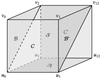
Figure 1: A cube with three quadrilateral faces labelled by ${\mathcal{A}}$, ${\mathcal{C}}$ and ${\mathcal{C}}^{\prime}$, an interior diagonal quadrilateral labelled by ${\mathcal{S}}$ and triangular domains labelled as ${\mathcal{B}}$ and ${\mathcal{B}}^{\prime}$. Note that primes denote domains on parallel faces.

Correspondingly, we define polynomials of 4 variables $\mathcal{A},\mathcal{S},\mathcal{C},\mathcal{C}^{\prime}\colon\mathbb{C}^{4}\to\mathbb{C}$ and those of 3 variables $\mathcal{B},\mathcal{B}^{\prime}\colon\mathbb{C}^{3}\to\mathbb{C}$, such that $\mathcal{B}$ and $\mathcal{B}^{\prime}$ written as functions of $(x,y,z)$ satisfy

1. $\deg_{x}{\mathcal{B}}\geq 1$, $\deg_{y}{\mathcal{B}}=\deg_{z}{\mathcal{B}}=1$;

2. the equation ${\mathcal{B}}=0$ can be solved for $y$ and $z$, and each solution is a rational function of the other two arguments.

With the labelling of vertices given in Figure 1, we denote the system of six corresponding equations by

$${\mathcal{A}}(u_{0},u_{1},u_{2},u_{12})=0,\qquad {\mathcal{S}}(u_{0},u_{1},v_{2},v_{12})=0,$$ (A.1a)

$${\mathcal{B}}(u_{0},v_{0},v_{2})=0,\qquad {\mathcal{B}}^{\prime}(u_{1},v_{1},v_{12})=0,$$ (A.1b)

$${\mathcal{C}}(u_{0},u_{1},v_{0},v_{1})=0,\qquad {\mathcal{C}}^{\prime}(u_{2},u_{12},v_{2},v_{12})=0.$$ (A.1c)

The following definition describes how consistency holds for this system of equations.

Definition A.1 (CABC property).

Let $\{u_{0},u_{1},u_{2},v_{0}\}$ be given initial values. Using equations (A.1), we can express the variable $v_{12}$ as a rational function in terms of the initial values in 3 ways. When the 3 results for $v_{12}$ are equal, the system of equations (A.1) is said to be consistent around a broken cube or to have the consistency around a broken cube (CABC) property. In this case, we refer to the configuration of quadrilaterals and triangular domains associated with the polynomials $\mathcal{A}$, $\mathcal{S}$, $\mathcal{C}$, $\mathcal{C}^{\prime}$, $\mathcal{B}$, $\mathcal{B}^{\prime}$ as a CABC cube.

Other equations arise from interrelationships between the above equations on the broken cube. For example, an equation arises on the top face, parallel to $\mathcal{A}$. It is also useful to note equations that relate three vertices on a face to a vertex on the opposite face. The following definition of such equations uses terminology analogous to existing ones in the literature on the CAC property.

Definition A.2 (tetrahedron property).

A CABC cube is said to have a tetrahedron property, if there exist quad-equations ${\mathcal{K}}_{1}$ and ${\mathcal{K}}_{2}$ satisfying

$${\mathcal{K}}_{1}(u_{0},u_{1},v_{0},v_{12})=0,\qquad{\mathcal{K}}_{2}(u_{0},u_{1},v_{1},v_{2})=0.$$

In this case, each of the equations ${\mathcal{K}}_{1}=0$ and ${\mathcal{K}}_{2}=0$ is referred to as a tetrahedron equation.

By interpreting each vertex value as an iterate of a function in an appropriate way, we can interpret the above equations as P$\Delta$Es. In particular, we use the terminology given in equation (1.4) for $u_{l,m}$ and $v_{l,m}$ to give the following definition of P$\Delta$Es.

Definition A.3 (CABC and tetrahedron properties for a system of P$\Delta$Es).

Define the P$\Delta$Es

$${\mathsf{A}}\bigl{(}u,\overline{u},\widetilde{u},\widetilde{\overline{u}}\bigl{)}=0,\qquad{\mathsf{S}}\big{(}u,\overline{u},\widetilde{v},\widetilde{\overline{v}}\big{)}=0,\qquad{\mathsf{B}}\big{(}u,v,\widetilde{v}\big{)}=0,\qquad{\mathsf{C}}\big{(}u,\overline{u},v,\overline{v}\big{)}=0,$$ (A.2)

which give the following equations around each elementary cubic cell in $\mathbb{Z}^{3}$:

$$\mathcal{A}={\mathsf{A}}\bigl{(}u,\overline{u},\widetilde{u},\widetilde{\overline{u}}\bigl{)}=0,\qquad \mathcal{S}={\mathsf{S}}\big{(}u,\overline{u},\widetilde{v},\widetilde{\overline{v}}\big{)}=0,$$ (A.3a)

$${\mathcal{B}}={\mathsf{B}}\big{(}u,v,\widetilde{v}\big{)}=0,\qquad {\mathcal{B}}^{\prime}={\mathsf{B}}\big{(}\overline{u},\overline{v},\widetilde{\overline{v}}\big{)}=0,$$ (A.3b)

$${\mathcal{C}}={\mathsf{C}}\big{(}u,\overline{u},v,\overline{v}\big{)}=0,\qquad {\mathcal{C}}^{\prime}={\mathsf{C}}\big{(}\widetilde{u},\widetilde{\overline{u}},\widetilde{v},\widetilde{\overline{v}}\big{)}=0.$$ (A.3c)

Then, the system (A.2) is said to have the CABC property if Definition A.1 holds for the equations (A.3). We also transfer the definition of tetrahedron properties to P$\Delta$Es corresponding to $\mathcal{K}_{j}$, $j=1,2$, in the obvious way. Moreover, the P$\Delta$E

$${\mathsf{A}}\bigl{(}u,\overline{u},\widetilde{u},\widetilde{\overline{u}}\bigl{)}=0$$

will be described as having the CABC property, if the system (A.2) has the CABC property.

Remark A.4.

Note that equations (A.2) are not necessarily autonomous. They may contain parameters that evolve with $(l,m)$.

Acknowledgment

This research was supported by a JSPS KAKENHI Grant Number JP19K14559.

References

• [1] Adler V.E., Bobenko A.I., Suris Yu.B., Classification of integrable equations on quad-graphs. The consistency approach, Comm. Math. Phys. 233 (2003), 513–543, arXiv:nlin.SI/0202024.
• [2] Adler V.E., Bobenko A.I., Suris Yu.B., Discrete nonlinear hyperbolic equations: classification of integrable cases, Funct. Anal. Appl. 43 (2009), 3–17, arXiv:0705.1663.
• [3] Bobenko A., Kutz N., Pinkall U., The discrete quantum pendulum, Phys. Lett. A 177 (1993), 399–404.
• [4] Bobenko A.I., Suris Yu.B., Integrable systems on quad-graphs, Int. Math. Res. Not. 2002 (2002), 573–611, arXiv:nlin.SI/0110004.
• [5] Boll R., Classification of 3D consistent quad-equations, J. Nonlinear Math. Phys. 18 (2011), 337–365, arXiv:1009.4007.
• [6] Boll R., Corrigendum: Classification of 3D consistent quad-equations, J. Nonlinear Math. Phys. 19 (2012), 1292001, 3 pages.
• [7] Capel H.W., Nijhoff F.W., Papageorgiou V.G., Complete integrability of Lagrangian mappings and lattices of KdV type, Phys. Lett. A 155 (1991), 377–387.
• [8] Hietarinta J., Joshi N., Nijhoff F.W., Discrete systems and integrability, Cambridge Texts in Applied Mathematics, Cambridge University Press, Cambridge, 2016.
• [9] Joshi N., Nakazono N., On the three-dimensional consistency of Hirota’s discrete Korteweg–de Vries equation, Stud Appl. Math. 147 (2021), 1409–1424, arXiv:2102.00684.
• [10] Kajiwara K., Ohta Y., Bilinearization and Casorati determinant solution to the non-autonomous discrete KdV equation, J. Phys. Soc. Japan 77 (2008), 054004, 9 pages, arXiv:0802.0757.
• [11] Kassotakis P., Nieszporski M., Difference systems in bond and face variables and non-potential versions of discrete integrable systems, J. Phys. A: Math. Theor. 51 (2018), 385203, 21 pages, arXiv:1710.11111.
• [12] Nakazono N., Discrete Painlevé transcendent solutions to the multiplicative type discrete KdV equations, J. Math. Phys., to appear, arXiv:2104.11433.
• [13] Nijhoff F.W., Lax pair for the Adler (lattice Krichever–Novikov) system, Phys. Lett. A 297 (2002), 49–58, arXiv:nlin.SI/0110027.
• [14] Nijhoff F.W., Capel H.W., Wiersma G.L., Quispel G.R.W., Bäcklund transformations and three-dimensional lattice equations, Phys. Lett. A 105 (1984), 267–272.
• [15] Nijhoff F.W., Quispel G.R.W., Capel H.W., Direct linearization of nonlinear difference-difference equations, Phys. Lett. A 97 (1983), 125–128.
• [16] Nijhoff F.W., Walker A.J., The discrete and continuous Painlevé VI hierarchy and the Garnier systems, Glasg. Math. J. 43A (2001), 109–123, arXiv:nlin.SI/0001054.
• [17] Nimmo J.J.C., Schief W.K., An integrable discretization of a $(2+1)$-dimensional sine-Gordon equation, Stud. Appl. Math. 100 (1998), 295–309.
• [18] Quispel G.R.W., Nijhoff F.W., Capel H.W., van der Linden J., Linear integral equations and nonlinear difference-difference equations, Phys. A 125 (1984), 344–380.
• [19] Tremblay S., Grammaticos B., Ramani A., Integrable lattice equations and their growth properties, Phys. Lett. A 278 (2001), 319–324, arXiv:0709.3095.
• [20] Volkov A.Yu., Faddeev L.D., Quantum inverse scattering method on a spacetime lattice, Theoret. and Math. Phys. 92 (1992), 837–842.
• [21] Walker A., Similarity reductions and integrable lattice equations, Ph.D. Thesis, University of Leeds, 2001.
\LastPageEnding