Semantic Code Classification for Automated Machine Learning

Abstract

A range of applications for automatic machine learning need the generation process to be controllable. In this work, we propose a way to control the output via a sequence of simple actions, that are called semantic code classes. Finally, we present a semantic code classification task and discuss methods for solving this problem on the Natural Language to Machine Learning (NL2ML) dataset.

1 Introduction

Code generation has the potential to be useful in a range of applications, although there is a variety of limitations (Chen et al. (2021)). Despite the recent success in this area with Codex models (Chen et al. (2021)), controlled code generation remains challenging (Xu et al. (2021); Hu et al. (2017)). Code generation models usually receive a code prompt (Feng et al. (2020); Chen et al. (2021) or a description of a task in natural language (Clement et al. (2020)), but the output is not controlled.

Automatic machine learning (AutoML) is a specialized area of code generation. Controlled generation of machine learning (ML) code is crucial for AutoML applications because code requirements for the same task may vary drastically in practice. Some applications focus more on interpretability; others might be satisfied with uninterpretable models that perform well.

Many machine learning programs follow a specific sequence of steps. Such sequence is called an ML pipeline. Every machine learning program may be roughly split into code snippets, such that each snippet is responsible for a single small action. These small actions are called semantic code classes.

A sequence of semantic classes can control the generation process and provide a generative model with additional information about the requested pipeline. Such a sequence serves as a guide and indicates the most important steps.

Training a model to recognize a sequence of semantic actions requires a labeled dataset. The labeling task is highly specific and requires a lot of manual labor, hence it might be beneficial to train an additional model for labeling.

In this work, we present the semantic code classification task and compare the results of various models. Such representation allows to better understand the structure of the ML code and the contents of each step of possible pipelines.

2 Dataset

Natural Language to Machine Learning (NL2ML) corpus is a collection of code blocks from Kaggle competition notebooks. It includes 101 071 different notebooks comprising 2 587 074 cells (or code block), which participants submitted to 266 Kaggle competitions. 4 748 of those code blocks have passed through manual assessment of its semantics. Each block is attributed to an upper-level category, which corresponds to a coarse meaning, and a second-level category, representing the finer semantic of that block. Publication of the corpus, along with the detailed description of the annotation process, is delayed due to legal considerations with Kaggle.

The upper level categories attribute the general kind of code block. One block can belong to a single category. Here is the list of possible values: Hypothesis, Environment, Data extraction, Exploratory data analysis, Data transform, Model train, Model evaluation, Model interpretation, Hyperparameter tuning, Visualization. The lower-level category represents a more specific type, for example, upper-level class Data transform contains such items as create dataframe, remove duplicates, correct missing values, feature engineering, filter and others.

The dataset is very unbalanced (appendix 1). Some simple classes (show table) are overrepresented because data contains many similar examples. At the same time, many classes (load data from zip, remove duplicates) are represented by less than 10 examples. Another difficulty is that data is heavily skewed because a large portion of the snippets came from the same competition; hence the snippets in the same class tend to be similar in general.

3 Code classification

This section describes methods we used to classify code blocks into the lower level semantic classes. The details about metric computation are provided in the section 4. For all models except neural networks we provide metrics with error bars that measure randomness in training the model.

The source code is available online.

3.1 Baseline solution: SVM

Support vector machines classifier (Boser et al. ) with linear kernel was used as baseline solution because the method does not require a large amount of samples. The multiclass support is handled according to a one-vs-one scheme (Chang & Lin (2011)). Baseline F1-score is 0.676 $\pm$ 0.029.

The F1-score is defined by the following formula:

$$F_{1}=2\frac{precision\cdot recall}{precision+recall}$$

Due to the imbalance in the data, the F1-score was chosen as the target metric.

3.2 Preprocessing

All the code blocks were modified according to PEP8 using a standard Python utility, autopep8, to eliminate the problems with code-style differences.

Comments have been removed from the code. Despite the fact that they can contain a lot of information about the block’s semantic type, their presence, as a rule, slightly degrades the quality of predictions. This is most likely because the content of the comments can be both useful and confusing. The text may contain information unrelated to the code block or unnecessary code that does not affect the semantic type.

For tokenization, the Byte-pair encoding method was used (Sennrich et al. (2015)). The tokenizer was trained using unlabeled data. The size of the dictionary used is 30,000 tokens; during the training, the BPE-Dropout regularization technique was used (Provilkov et al. (2019)).

This tokenization has proven to be quite helpful for many models. The names of entities in the program code can consist of several words, written together or through an underscore "_". Splitting by the spaces cannot distinguish different words included in the names of entities, and breaking into n-grams may not be flexible since words in names can have different lengths. The BPE method was optimal because it can extract information about the donkeys that are often found in the names of entities.

Term frequency-inverse document frequency (TF-IDF) (Zhang et al. (2011)) was used as features for models. These statistics show the importance of the token in the document, given the context of the corpus.

3.3 Naive Bayesian Classifier and NB-SVM

The Naive Bayesian Classifier (NB) (Raschka (2014)) is a probabilistic model based on Bayes’ theorem. NB Classifier is a common pre-neural network method for classifying text data. As a rule, it is assumed that the data has either a multinomial distribution or a Bernoulli distribution.

Since the dataset is unbalanced, estimates for the parameters of the multinomial distribution may be unstable, which negatively affects the quality of predictions. To combat this problem, a complementary NB was proposed in Rennie et al. (2003).

The model with the Bernoulli distribution showed the best result among naive Bayesian classifiers. This is because this model works best with short texts (Mccallum & Nigam (2001)). Short texts predominate in the training dataset.

Metrics for NB classifier are in rows Multinomial NB, Complementary NB, Bernoulli NB of table 2.

NB classifier and SVM are often used as basic solutions in text classification problems. NB tends to perform better on shorter passages, while SVM works best on longer texts. The article Wang & Manning (2012) discusses the composition of an NB classifier and SVM, Naive Bayes - Support Vector Machine (NBSVM), which combines the advantages of both methods. The paper also states that binarization of NB features or using bigrams should improve results, but in our case it’s the opposite. Metrics for NBSVM classifier are in rows NBSVM, NBSVM (binarization), NBSVM birams of table 2.

3.4 Neural networks

Neural networks are an important class of machine learning algorithms. It is due to neural networks that the quality of text data processing has been improved. Unfortunately, many advanced neural network architectures require a lot of training data. There was not too much data in this case, but it was possible to obtain relatively good results.

There is not enough data to train vector representations, so frozen pretrained CodeBERT (Feng et al. (2020)) was used. CodeBERT has several drawbacks that are worth noting. Firstly, the important thing is that this model uses its own tokenizer. The tokens used do not quite match the machine learning code as they were derived from more general code, which means that machine learning-specific tokens may be too rare to enter the dictionary. Secondly, CodeBERT was trained on the program code not only in Python3 but also in several other languages: JavaScript, Java, PHP, Ruby, Go. Due to this, the connection of tokens with machine learning is becoming even less.

Another important point when training a neural network is the loss function, on which the success of the model depends a lot. The standard loss function in a classification problem is cross-entropy. Conventional cross-entropy is unstable to unbalanced data; the situation can be improved by adding weights for examples from different classes. Since there are a lot of classes, a vast number of hyperparameters appear, which is a big drawback since neural networks take a long time to learn.

For unbalanced data, there are alternative loss functions:

1. Soft-F1. This loss function directly optimizes the target metric in the task at hand, which is a significant advantage.

   The critical drawback of this loss function is that it requires a sizeable mini-batch size. If the batch size is too small, rare classes will often not be included in the batch, hence the precision and the recall are equal to 1, which is the optimal value for these metrics. If there are many such rare classes, the loss function will be extremely close to the optimum, leading to the fact that learning does not occur. In the dataset, quite a few classes contain less than 10 objects, which means that large batch size is required.

2. Focal Loss. This loss function comes from computer vision (Lin et al. (2017)). The main idea is to adaptively reduce the weight of objects for which the model determines the class correctly and confidently. Due to this, it is possible to learn patterns even in rare classes.

The following architectures were used:

1. Recurrent neural network (RNN). GRU and LSTM were tried as a recurrent layer; the result is approximately the same. The recurrent network is bidirectional, since this configuration usually gives the best result, allowing more context for the tokens. Row RNN in results table (2).

   The token sequence is fed into the inputs of the recurrent layer. The output goes through a dense layer, GELU activation, dropout, and outputs probabilities through dense layer and Softmax.

   Layer sizes are optimized with random search. The model with the best score uses a single LSTM layer with hidden state size of 180 and a hidden fully connected layer of size 269. The scheme is in appendix 2.

2. RNN with additive attention (Bahdanau et al. (2014)). The model differs from the usual RNN in only one layer: the attention layer added after the recurrent layer.

   The sizes of all layers were optimized using random search. The best model uses a single LSTM layer with hidden state size of 100. After attention, there is a hidden fully connected layer of size 135. The scheme of the model can be found in appendix 3.

   A layer of attention helps to identify the most important values in a sequence, which leads to a dramatic improvement in the result. Row RNN+Attention in results table (2).

3.5 Augmentation

Since the marked-up data is insufficient, augmentation was used. However, it is necessary that the code remains compilable and belongs to the same semantic type after modifications.

Many code blocks contain similar variable names (eg. "df", "train", "test"). They do not always provide additional information about the block type, but due to the frequency they are used by the classifier. Therefore, augmentation was applied, which masks some fraction of the variables in the block. the augmentation does not change the semantic of the block, as the names of user-defined variables can be almost anything. The variables in code were found using AST trees and replaced by masks, each variable in a block with a different one.

The augmentation was used with SVM and Attention RNN. Results are in rows SVM+Augmentation, RNN+Attention+Augmentation in table (2). The results have not improved enough(the value is within error bars), so we do not use augmentations in other experiments.

3.6 Hierarchy

The structure by which the code snippets are classified is a two-level graph: the first is the general class of action, the second is what exactly is done in the block. Therefore, it was decided to implement this structure as a two-level classifier, where the upper vertex is predicted first, and then the lower by a separate classifier, already trained on specific objects belonging to the child vertices.

The advantage of considering the upper classes separately is that in contrast to the original dataset, each class is represented by at least several dozen objects. At the same time, most of the very small original classes go into such a classification together with other small classes. Thus, the determination of their upper class is a more realistic task. If we correctly guessed the upper class, then small objects are likely to have no large competitors. However, if the class was identified incorrectly in the first step, the subsequent classification is guaranteed to be inaccurate.

SVM was chosen as the lower classifier since the model demonstrated the best results in previous experiments, while the upper classifiers were

1. RNN containing a bidirectional LSTM, the vector representations were taken from the frozen pre-trained CodeBERT (Feng et al. (2020)).

2. SVM

In table 1 the metrics of the upper level classification are presented. SVM achieved sufficient results. The overall results of hierarchy classifier are in 2 - rows RNN + SVM Hierarchy, SVM + SVM Hierarchy - this method allowed to significantly improve metrics.

Table 1: Upper level prediction results.

	Metrics
Model	F1-score	Accuracy
RNN	0.759	0.773
SVM	0.937	0.938

3.7 Semi-supervised, pseudo labels

Since the amount of labeled data is extremely small, it was decided to experiment with semi-supervised models that allow to use unlabeled data (Xie et al. (2019)).

First, we trained a classic SVM model on the marked-up dataset. It’s predictions on unlabeled data were used as pseudo labels. Then another SVM model with separately selected hyperparameters was trained on pseudo-labeled data and a part of marked-up data. It was tested on the rest of the labeled data.

We tested this approach using 20%, 40%, and 100% of unlabeled data. The results are in rows Pseudo labels 20%, Pseudo labels 40%, Pseudo labels 100% in table (2).

4 Results

We evaluated models on marked-up code snippets of the NL2ML dataset. Several approaches demonstrated some improvements in metrics from the baseline solution. All of the resulting models are compared in the table (2) by F1-score and accuracy. The best results are achieved by hierarchy and pseudo-labels models. The first one utilizes the knowledge of the classes structure, and the second one uses a great amount of unlabeled data.

The target metrics were computed on a test dataset that contains 20 % of all labeled data. For each model, we optimized hyperparameters with random search. For neural networks, we used a validation set that contains 20 % of labeled data. For other methods, we used cross-validation with 10 folds.

Table 2: Summary table of all the models and their results

	Metrics
Model	F1-score	Accuracy
SVM+Linear (Baseline)	0.676 $\pm$ 0.029	0.678 $\pm$ 0.031
SVM + Poly	0.620 $\pm$ 0.033	0.627 $\pm$ 0.030
SVM + RBF	0.672 $\pm$ 0.031	0.676 $\pm$ 0.031
Multinomial NB	0.561 $\pm$ 0.031	0.583 $\pm$ 0.031
Complementary NB	0.576 $\pm$ 0.024	0.587 $\pm$ 0.023
Bernoulli NB	0.609 $\pm$ 0.021	0.623 $\pm$ 0.026
NBSVM	0.694 $\pm$ 0.013	0.704 $\pm$ 0.015
NBSVM (binarization)	0.684 $\pm$ 0.016	0.694 $\pm$ 0.015
NBSVM (bigrams)	0.689 $\pm$ 0.14	0.697 $\pm$ 0.14
RNN	0.541	0.556
RNN + Attention	0.639	0.648
SVM + Augmentation	0.686 $\pm$ 0.031	0.696 $\pm$ 0.029
RNN + Attention + Augmentation	0.638	0.652
RNN + SVM Hierarchy	0.291	0.282
SVM+SVM Hierarchy	0.741	0.744
Pseudo labels 20 %	0.713 $\pm$ 0.014	0.724 $\pm$ 0.014
Pseudo labels 40 %	0.727 $\pm$ 0.016	0.738 $\pm$ 0.014
Pseudo labels 100 %	0.755 $\pm$ 0.03	0.764 $\pm$ 0.028

5 Conclusion

This paper compares methods for semantic classification of code snippets from NL2ML corpus, a large-scale dataset of data science-specific code harvested from Kaggle, the largest platform for data science competitions. The dataset includes only 4 748 manually labeled snippets.

We provided detailed qualitative and quantitative comparisons of the used classification methods. The final proposed model demonstrated better results than the baseline SVM solution, which has an F1-score of 0.67. The method with the best F1-score of 0.755 is an SVM trained on pseudo-labels.

The proposed method allows to automatically markup a program code corpus with better accuracy and performance, as well as effectively assess the quality of data science code in Python. We also genuinely hope that this work can contribute to the development of the next generation of robust AutoML systems, as semantic classification provides an interlingua that can be used for translating between natural and programming languages.

Appendix A Distribution of snippets by semantic types

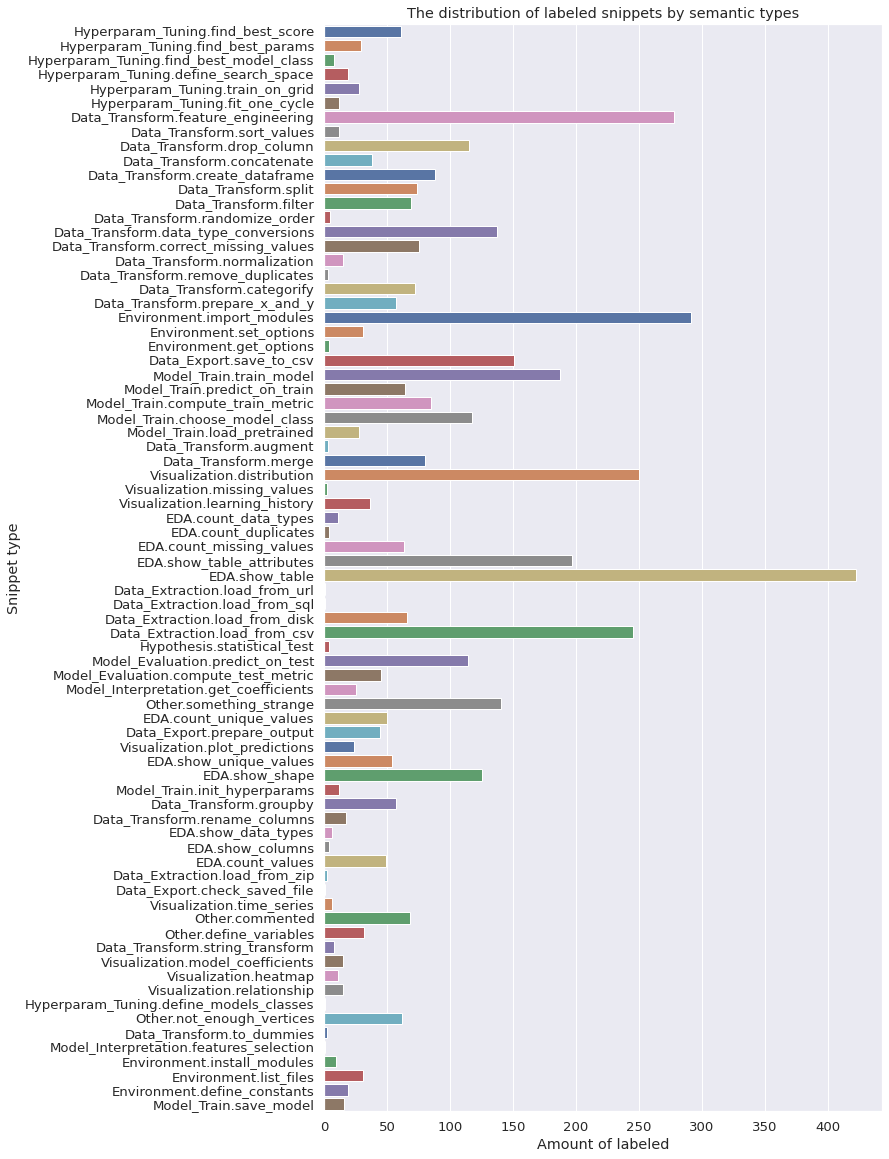
Figure 1: The distribution of labeled snippets by semantic types.

Appendix B Architectures of neural nets

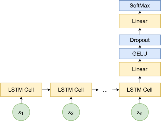
Figure 2: Architecture of recurrent neural network

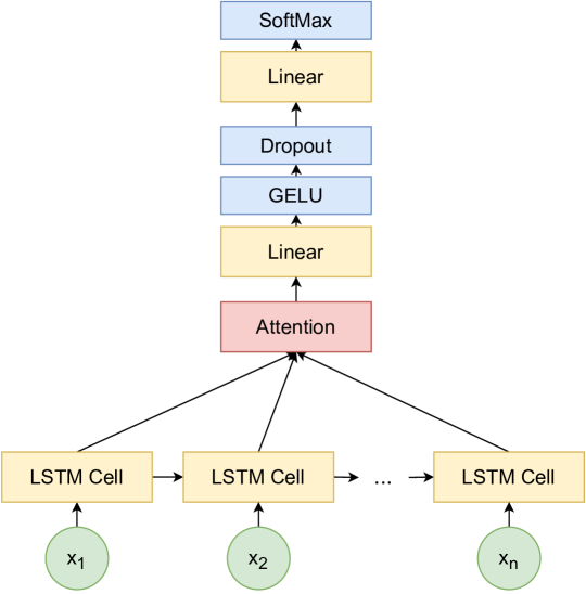
Figure 3: Architecture of recurrent neural network with attention

Appendix C Code snippets

Table 3: Examples of code snippets from NL2ML dataset

Semantic class	Example
⬇ train_df.drop("Date", inplace=True, axis=1) test_df.drop("Date", inplace=True, axis=1)
⬇ from sklearn import linear_model reg_CC = linear_model.Lasso(alpha=0.1) reg_Fat = linear_model.Lasso(alpha=0.1)
⬇ parameters = {’lstm_nodes’: [14,16,20], ’nb_epoch’: [50], ’batch_size’: [32], ’optimizer’: [’adam’]}
⬇ fig = plt.figure() fig.suptitle("Algorithm␣Comparison") ax = fig.add_subplot(111) plt.boxplot(results) ax.set_xticklabels(names) plt.show()
⬇ scaler = MinMaxScaler() df[’revenue’] = scaler.fit_transform( df[[’revenue’]] )
⬇ rfr = RandomForestRegressor( n_estimators=200, max_depth=5, max_features=0.5, random_state=449, n_jobs=-1 ) rfr.fit(x_train, y_train)

Appendix D Selected hyperparameters for each model

Table 4: Hyperparameters for models without hierarchy and first level of hierarchical models

Model	Hyperparameter	Type	Value
SVM+Linear (Baseline)	C	numeric	37.17
	min_df for TF-IDF	integer	2
	max_df for TF-IDF	numeric	0.31
SVM + Poly	C	numeric	1.43
	Degree of poly kernel	integer	3
	min_df for TF-IDF	integer	6
	max_df for TF-IDF	numeric	0.30
SVM + RBF	C	numeric	8.71
	min_df for TF-IDF	integer	7
	max_df for TF-IDF	numeric	0.39
Multinomial NB	Alpha	numeric	0.01
	min_df for TF-IDF	integer	2
	max_df for TF-IDF	numeric	0.57
Complementary NB	Alpha	numeric	0.29
	min_df for TF-IDF	integer	2
	max_df for TF-IDF	numeric	0.30
Bernoulli NB	Alpha	numeric	0.01
	min_df for TF-IDF	integer	5
	max_df for TF-IDF	numeric	0.30
NBSVM	C for SVM	numeric	0.50
	Kernel type	categorical	Linear
	Alpha for Naive Bayes	numerical	4.22
	min_df for TF-IDF	integer	1
	max_df for TF-IDF	numeric	0.94
NBSVM (binarization)	C for SVM	numeric	0.10
	Kernel type	categorical	Linear
	Alpha for Naive Bayes	numerical	0.28
	min_df for TF-IDF	integer	3
	max_df for TF-IDF	numeric	0.94
NBSVM (bigrams)	C for SVM	numeric	0.10
	Kernel type	categorical	Linear
	Alpha for Naive Bayes	numerical	2.51
	min_df for TF-IDF	integer	2
	max_df for TF-IDF	numeric	0.95
RNN	RNN cell type	categorical	LSTM
	Size of hidden state	integer	180
	Size of linear layer	integer	269
RNN + Attention	RNN cell type	categorical	LSTM
	Size of hidden state	integer	100
	Size of linear layer	integer	135
SVM + Augmentation	C	numeric	5.82
	Kernel type	categorical	Linear
	min_df for TF-IDF	integer	2
	max_df for TF-IDF	numeric	0.30
	Percent of masked variables	numeric	0.93
RNN + Attention + Augmentation	RNN cell type	categorical	LSTM
	Size of hidden state	integer	169
	Size of linear layer	integer	255
	Percent of masked variables	numeric	99.7%
SVM+SVM Hierarchy (1st level)	C	numeric	149.65
	Kernel type	categorical	Poly
	Degree of poly kernel	integer	2
RNN+SVM Hierarchy (1st level)	RNN cell type	categorical	LSTM
	Size of hidden state	integer	143
	Size of linear layer	integer	185
Pseudo labels 20 %	C	numeric	98.37
	Kernel type	categorical	linear
	min_df for TF-IDF	integer	3
	max_df for TF-IDF	numeric	0.53
Pseudo labels 40 %	C	numeric	121.59
	Kernel type	categorical	linear
	min_df for TF-IDF	integer	3
	max_df for TF-IDF	numeric	0.41
Pseudo labels 100%	C	numeric	145.56
	Kernel type	categorical	linear
	min_df for TF-IDF	integer	2
	max_df for TF-IDF	numeric	0.26

Table 5: Hyperparameters for SVM+SVM Hierarchy (2nd level). Separate parameters for each upper level class. If upper level class is not present in this table, then it has one subclass and hence does not require a second level classificator.

Upper level class	Hyperparameter	Type	Value
Data Extraction	C	numeric	135.49
	Kernel type	categorical	Linear
	min_df for TF-IDF	integer	50
	max_df for TF-IDF	numeric	0.89
EDA	C	numeric	4.70
	Kernel type	categorical	Linear
	min_df for TF-IDF	integer	4
	max_df for TF-IDF	numeric	0.61
Environment	C	numeric	232.06
	Kernel type	categorical	Linear
	min_df for TF-IDF	integer	6
	max_df for TF-IDF	numeric	0.81
Model_Train	C	numeric	9.63
	Kernel type	categorical	RBF
	min_df for TF-IDF	integer	17
	max_df for TF-IDF	numeric	0.47
Data_Transform	C	numeric	298.83
	Kernel type	categorical	Linear
	min_df for TF-IDF	integer	2
	max_df for TF-IDF	numeric	0.20
Model_Evaluation	C	numeric	0.84
	Kernel type	categorical	Poly
	Degree of poly kernel	integer	3
	min_df for TF-IDF	integer	16
	max_df for TF-IDF	numeric	0.50
Data_Export	C	numeric	5.35
	Kernel type	categorical	RBF
	min_df for TF-IDF	integer	23
	max_df for TF-IDF	numeric	0.83
Hyperparam_Tuning	C	numeric	20.03
	Kernel type	categorical	RBF
	min_df for TF-IDF	integer	6
	max_df for TF-IDF	numeric	0.26
Visualization	C	numeric	865.58
	Kernel type	categorical	Linear
	min_df for TF-IDF	integer	2
	max_df for TF-IDF	numeric	0.66

Table 6: Hyperparameters for RNN+SVM Hierarchy (2nd level). Separate parameters for each upper level class. If upper level class is not present in this table, then it has one subclass and hence does not require a second level classificator.

Upper level class	Hyperparameter	Type	Value
Data Extraction	C	numeric	7.66
	Kernel type	categorical	RBF
	min_df for TF-IDF	integer	17
	max_df for TF-IDF	numeric	0.88
EDA	C	numeric	1.71
	Kernel type	categorical	Linear
	min_df for TF-IDF	integer	6
	max_df for TF-IDF	numeric	0.32
Environment	C	numeric	462.65
	Kernel type	categorical	RBF
	min_df for TF-IDF	integer	16
	max_df for TF-IDF	numeric	0.87
Model_Train	C	numeric	4.58
	Kernel type	categorical	Linear
	min_df for TF-IDF	integer	1
	max_df for TF-IDF	numeric	0.90
Data_Transform	C	numeric	204.62
	Kernel type	categorical	Linear
	min_df for TF-IDF	integer	2
	max_df for TF-IDF	numeric	0.45
Model_Evaluation	C	numeric	2.03
	Kernel type	categorical	Linear
	min_df for TF-IDF	integer	3
	max_df for TF-IDF	numeric	0.63
Data_Export	C	numeric	26.49
	Kernel type	categorical	Poly
	Degree of poly kernel	numeric	2
	min_df for TF-IDF	integer	23
	max_df for TF-IDF	numeric	0.93
Hyperparam_Tuning	C	numeric	14.58
	Kernel type	categorical	Linear
	min_df for TF-IDF	integer	10
	max_df for TF-IDF	numeric	0.65
Visualization	C	numeric	2.48
	Kernel type	categorical	Linear
	min_df for TF-IDF	integer	2
	max_df for TF-IDF	numeric	0.21

References

- Bahdanau et al. (2014) Dzmitry Bahdanau, Kyunghyun Cho, and Yoshua Bengio. Neural machine translation by jointly learning to align and translate. arXiv preprint arXiv:1409.0473, 2014.
- (2) Bernhard E Boser, Isabelle M Guyon, and Vladimir N Vapnik. A training algorithm for optimal margin classifiers. In Proceedings of the 5th Annual ACM Workshop on Computational Learning Theory, pp. 144–152.
- Chang & Lin (2011) Chih-Chung Chang and Chih-Jen Lin. Libsvm: a library for support vector machines. ACM transactions on intelligent systems and technology (TIST), 2(3):1–27, 2011.
- Chen et al. (2021) Mark Chen, Jerry Tworek, Heewoo Jun, Qiming Yuan, Henrique Ponde de Oliveira Pinto, Jared Kaplan, Harrison Edwards, Yuri Burda, Nicholas Joseph, Greg Brockman, Alex Ray, Raul Puri, Gretchen Krueger, Michael Petrov, Heidy Khlaaf, Girish Sastry, Pamela Mishkin, Brooke Chan, Scott Gray, Nick Ryder, Mikhail Pavlov, Alethea Power, Lukasz Kaiser, Mohammad Bavarian, Clemens Winter, Philippe Tillet, Felipe Petroski Such, Dave Cummings, Matthias Plappert, Fotios Chantzis, Elizabeth Barnes, Ariel Herbert-Voss, William Hebgen Guss, Alex Nichol, Alex Paino, Nikolas Tezak, Jie Tang, Igor Babuschkin, Suchir Balaji, Shantanu Jain, William Saunders, Christopher Hesse, Andrew N. Carr, Jan Leike, Joshua Achiam, Vedant Misra, Evan Morikawa, Alec Radford, Matthew Knight, Miles Brundage, Mira Murati, Katie Mayer, Peter Welinder, Bob McGrew, Dario Amodei, Sam McCandlish, Ilya Sutskever, and Wojciech Zaremba. Evaluating large language models trained on code. CoRR, abs/2107.03374, 2021. URL https://arxiv.org/abs/2107.03374.
- Clement et al. (2020) Colin B. Clement, Dawn Drain, Jonathan Timcheck, Alexey Svyatkovskiy, and Neel Sundaresan. Pymt5: multi-mode translation of natural language and python code with transformers. CoRR, abs/2010.03150, 2020. URL https://arxiv.org/abs/2010.03150.
- Feng et al. (2020) Zhangyin Feng, Daya Guo, Duyu Tang, Nan Duan, Xiaocheng Feng, Ming Gong, Linjun Shou, Bing Qin, Ting Liu, Daxin Jiang, and Ming Zhou. Codebert: A pre-trained model for programming and natural languages. CoRR, abs/2002.08155, 2020. URL https://arxiv.org/abs/2002.08155.
- Hu et al. (2017) Zhiting Hu, Zichao Yang, Xiaodan Liang, Ruslan Salakhutdinov, and Eric P. Xing. Controllable text generation. CoRR, abs/1703.00955, 2017. URL http://arxiv.org/abs/1703.00955.
- Lin et al. (2017) Tsung-Yi Lin, Priya Goyal, Ross B. Girshick, Kaiming He, and Piotr Dollár. Focal loss for dense object detection. CoRR, abs/1708.02002, 2017. URL http://arxiv.org/abs/1708.02002.
- Mccallum & Nigam (2001) Andrew Mccallum and Kamal Nigam. A comparison of event models for naive bayes text classification. Work Learn Text Categ, 752, 05 2001.
- Provilkov et al. (2019) Ivan Provilkov, Dmitrii Emelianenko, and Elena Voita. Bpe-dropout: Simple and effective subword regularization. CoRR, abs/1910.13267, 2019. URL http://arxiv.org/abs/1910.13267.
- Raschka (2014) Sebastian Raschka. Naive bayes and text classification I - introduction and theory. CoRR, abs/1410.5329, 2014. URL http://arxiv.org/abs/1410.5329.
- Rennie et al. (2003) Jason D. M. Rennie, Lawrence Shih, Jaime Teevan, and David R. Karger. Tackling the poor assumptions of naive bayes text classifiers. In Proceedings of the Twentieth International Conference on International Conference on Machine Learning, ICML’03, pp. 616–623. AAAI Press, 2003. ISBN 1577351894.
- Sennrich et al. (2015) Rico Sennrich, Barry Haddow, and Alexandra Birch. Neural machine translation of rare words with subword units. CoRR, abs/1508.07909, 2015. URL http://arxiv.org/abs/1508.07909.
- Wang & Manning (2012) Sida Wang and Christopher Manning. Baselines and bigrams: Simple, good sentiment and topic classification. In Proceedings of the 50th Annual Meeting of the Association for Computational Linguistics (Volume 2: Short Papers), pp. 90–94, Jeju Island, Korea, July 2012. Association for Computational Linguistics. URL https://aclanthology.org/P12-2018.
- Xie et al. (2019) Qizhe Xie, Eduard H. Hovy, Minh-Thang Luong, and Quoc V. Le. Self-training with noisy student improves imagenet classification. CoRR, abs/1911.04252, 2019. URL http://arxiv.org/abs/1911.04252.
- Xu et al. (2021) Frank F. Xu, Bogdan Vasilescu, and Graham Neubig. In-ide code generation from natural language: Promise and challenges. CoRR, abs/2101.11149, 2021. URL https://arxiv.org/abs/2101.11149.
- Zhang et al. (2011) Wen Zhang, Taketoshi Yoshida, and Xijin Tang. A comparative study of tf*idf, lsi and multi-words for text classification. Expert Systems with Applications, 38(3):2758–2765, 2011. ISSN 0957-4174. doi: https://doi.org/10.1016/j.eswa.2010.08.066. URL https://www.sciencedirect.com/science/article/pii/S0957417410008626.