Wigner - Weyl calculus in description of non - dissipative transport phenomena

Abstract

Application of Wigner - Weyl calculus to the investigation of non - dissipative transport phenomena is reviewed. We focus on the quantum Hall effect, Chiral Magnetic effect, and Chiral separation effect, and discuss the role of interactions, inhomogeneity, and deviations from equilibrium.

I Introduction

Wigner-Weyl calculus originates from the works of H. Groenewold [1] and J. Moyal [2]. It replaces the ordinary quantum mechanics by the quantum mechanics written using Weyl symbols of operators that are functions on phase space. The ideas realized in Wigner - Weyl calculus were proposed earlier by H. Weyl [3] and E. Wigner [4] themselves. In this formalism Weyl symbols are used instead of the the operators of physical quantities. The product of two operators is replaced by the Moyal product of two functions [5, 6]. This calculus has been applied to the solution of quantum mechanical problems [7, 8]. The most well - known problem of this type is the unharmonic oscillator. Within the quantum field theory the Wigner-Weyl formalism was applied to several problems of high energy physics theory and to condensed matter physics [9, 10, 11, 12, 13, 14, 15]. For the applications to QCD see [16, 17]. There were also numerous applications of this calculus to quantum kinetic theory [18, 19].

It is worth mentioning that it is not easy to extend Wigner-Weyl calculus to lattice models, although the attempts to built such a formalism started long time ago [20, 15, 21], see also [22, 23, 24, 25]. The so - called approximate version of the lattice Wigner-Weyl calculus has been proposed in the participation of the present author [26]. This calculus is approximate because its application is limited to the systems with weak inhomogeneity, which means, in particular, that the external magnetic field strength should be much smaller than $10000$ Tesla. In practise this requirement is always fulfilled in real solid state systems and in the lattice regularized relativistic quantum field theory. It appears that within this formalism one may express through the topological invariants the response of various nondissipative currents to external field strength [27, 28, 29, 30, 31, 32, 33].

The topological invariants considered in [27, 28, 29, 30, 31, 32, 33] are composed of the Green funcitons. The invariants of this kind were considered much more earlier. The simplest ones are responsible for the stability of the Fermi surface in the $3+1$ D systems:

$$N_{1}=\mathop{\rm tr}\nolimits\oint_{C}\frac{1}{2\pi\mathrm{i}}G(p_{0},{\bm{p}})dG^{-1}(p_{0},{\bm{p}}).$$ (1)

Here $C$ is an arbitrary contour, which encloses the Fermi surface [34] within momentum space. The topological stability of Fermi points is protected by [35, 34]

$$N_{3}=\frac{1}{24\pi^{2}}\epsilon_{\mu\nu\rho\lambda}\mathop{\rm tr}\nolimits\int_{S}dS^{\mu}G\partial^{\nu}G^{-1}G\partial^{\rho}G^{-1}G\partial^{\lambda}G^{-1}.$$ (2)

Here $S$ is the surface that surrounds the Fermi points.

The first topological expression for the Hall conductivity was given through the TKNN invariant [36]. This invariant has been defined for the systems in the presence of constant external magnetic field, and for the description of intrinsic anomalous quantum Hall effect in homogeneous systems [37, 38, 39, 40, 41]. Strictly speaking, the TKNN invariant may be applied only to the systems with constant magnetic field or homogeneous quantum Hall insulators. In the presence of interactions the TKNN invariant is not defined.

In the absence of interactions the TKNN invariant for the intrinsic QHE (existing without external magnetic field) may be re - written through the momentum space Green’s function [42, 43] (see also Chapter 21.2.1 in [34]). For the $2+1$D fermions the Hall conductivity is given by

$$\sigma_{H}=\frac{\cal N}{2\pi},$$

where

$${\cal N}=\frac{\epsilon_{ijk}}{\,3!\,4\pi^{2}}\,\int d^{3}p\mathop{{\rm Tr}}\nolimits\left[{G}(p)\frac{\partial{G}^{-1}(p)}{\partial p_{i}}\frac{\partial{G}(p)}{\partial p_{j}}\frac{\partial{G}^{-1}(p)}{\partial p_{k}}\right].$$ (3)

In the presence of interactions this expression remains valid, if the non-interacting two-point Green’s function has been substituted by the Green’s function with the interaction corrections [44, 45, 46]. The original TKNN invariant cannot be extended in a similar way to the interacting systems in principle.

In the present paper we review the recent works by the group working in Ariel University on the topological description of non - dissipative transport in non - homogeneous systems. We summarize here the results reported earlier in a series of papers (see [26, 47, 48, 49, 50, 51, 52, 53] and references therein). We used Wigner - Weyl formalism and start from the extension of Eq. (3) to the systems with weak inhomogeneity. In particular, such an inhomogeneity may be caused by disorder (in case of the solid state systems), or non - uniform external fields. It appears that the QHE conductivity remains topological even in this case. Moreover, we consider the perturbative corrections due to interactions. We will see that the QHE conductance remains robust to these corrections.

Another non - dissipative transport effect that will be considered in the present paper is the chiral magnetic effect (CME) [54, 55, 56, 57, 58]. It is widely believed that it does not appear in true equilibrium [59, 60, 61, 62, 63, 64, 65, 66]. It might appear out of equilibrium in a steady state with the chiral imbalance due to external electric field and external magnetic field [67]. Experimental detection of this effect was reported through the study of magnetoresistance in Dirac and Weyl semimetals [68]. In the absence of external electric field the chiral magnetic effect was predicted for the non - equilibrium systems with dependence on time in chiral chemical potential [69]. In the present paper we concern the setup of equilibrium CME in the presence of inhomogeneity, finite temperature and interactions. We will see that under these circumstances the CME still does not exist in equilibrium.

The chiral separation effect (CSE) was proposed in [70]. This is the appearance of an axial current in the direction of external magnetic field. In the chiral limit the axial current is proportional to the external magnetic field $B^{k}$ and the ordinary chemical potential $\mu$ counted from the Fermi point:

$${\bf J}_{5}=\frac{1}{2\pi^{2}}\mu{\bf B}$$ (4)

It was proposed to observe this effect in experiment during the heavy ion collisions [71, 72, 56, 73]. The quark - gluon plasma [74, 75, 76, 77, 78, 79, 80, 81, 82, 83, 84], presumably, appears within the fireballs resulted from the collisions of two heavy ions. Quarks in this state of matter are massless (if their current mass is neglected). Therefore, we deal with the chiral fermions. External magnetic field exists because the motion of ions creates electric currents. The non - central collisions produce strong magnetic field orthogonal to the trajectories of colliding ions. The CSE gives axial current within the fireball, which may be detected after the decay of the fireball indirectly through the distribution of outgoing particles. Relation between the CSE and the chiral anomaly has been discussed, for example, in [85]. The detailed consideration of the CSE may be found, for example, in [86, 62, 87]. Interaction corrections to CSE have been considered, for example, in [88]. The CSE was considered mostly for the homogeneous systems, while in any real experiments we deal with the inhomogeneous systems. Here we will concentrate on this situation and describe the CSE for the nonhomogeneous systems.

In order to extend our consideration to the systems out of equilibrium we use Keldysh formalism [89, 90, 91, 92, 93, 94, 95]. The finite temperature equilibrium quantum statistical mechanics [96, 97, 98, 99] and the real time QFT represent the limiting cases of Keldysh QFT. The functional integral formalism [100] as well as the operator formalism [101, 102] are used in Keldysh technique as well as in the equilibrium theory. The perturbation theory of Keldysh formalism is technically similar to the one of the conventional QFT [89, 101]. Schwinger-Dyson equations being applied to Keldysh technique [103, 104, 105, 94] provide the natural framework for the calculation of transport properties [106, 107, 108, 90, 91, 92, 101, 109, 110, 111, 102]. Keldysh formalism has been applied to QCD [112]. A version of Wigner-Weyl calculus similar to the one of equilibrium theory [53, 26] has been developed within the Keldysh formalism [113, 114, 115, 116, 117]. The gradient expansion together with the Schwwinger - Dyson equations here allows to calculate fermion propagator. In [118, 119] the development of this technique was given that allows to deal with the non - homogeneous systems. In the present paper we will discuss the further development of this line of research, and consider the application of Wigner - Weyl calculus to the non - dissipative transport phenomena for the systems out of equilibrium using an example of QHE.

The paper is organized as follows. In Sect. II we recall the basic notions of Wigner-Weyl calculus within the inhomogeneous theory at zero temperature. We follow here the approach of [26]. In Sect. III we consider the QHE at zero temperature [26] and equilibrium CME at finite temperature [51]. In Sect. IV we consider chiral separation effect and review results of [50]. In Sect. V we discuss loop corrections to the QHE conductivity of the two - dimensional non - homogeneous systems. We summarize here the results reported in [47] and [49]. In Sect. VI we briefly summarize the results of [52] on the QHE out of equilibrium. In Sect. VII we end with the conclusions.

II Wigner - Weyl calculus in equilibrium inhomogeneous theory.

II.1 Approximate Wigner - Weyl calculus

Here we closely follow [26]. We consider the lattice model with the partition function in momentum space at very small temperatures [120]

$$Z = \int D\bar{\psi}D\psi\,{\rm exp}\Big{(}\int_{\cal M}\frac{d^{D}{p}_{1}}{\sqrt{|{\cal M}|}}\int_{\cal M}\frac{d^{D}{p}_{2}}{\sqrt{|{\cal M}|}}\bar{\psi}^{T}({p}_{1}){\cal Q}(p_{1},p_{2})\psi({p}_{2})\Big{)},$$ (5)

Here $D$ is dimension of space - time. It is equal to $3$ if we are considering the two - dimensional systems, and $4$ if we are considering the three dimensional ones. Notice that we discretize imaginary time in the same way as spatial coordinates. For the condensed matter systems the lattice spacing in imaginary time direction is to be set to zero at the end of calculations, while the lattice spacing in spatial direction remains equal to the real distance between the adjacent lattice sites. For the lattice regularized relativistic quantum field theory the common lattice spacing is to be send to zero considering the continuum limit. By $|{\cal M}|$ we denote volume of $D$ - dimensional momentum space $\cal M$. Both $p_{1}$ and $p_{2}$ are $D$ - momenta. Here matrix elements of lattice Dirac operator $\hat{Q}$ are denoted by

$$\langle p_{1}|\hat{Q}|p_{2}\rangle={\cal Q}(p_{1},p_{2})$$

We use the units, in which both $\hbar$ and $c$ are equal to unity. Elementary charge of electron $e$ is included to the definition of electric and magnetic fields.

Wigner transformation of Green function ${\cal G}(p_{1},p_{2})=\langle p_{1}|\hat{G}|p_{2}\rangle$ that is the Weyl symbol of operator $\hat{G}$ is given by

$${G}_{W}(x,p)\equiv\int_{\cal M}dqe^{ixq}{\cal G}({p+q/2},{p-q/2})$$ (6)

Weyl symbol of operator $\hat{Q}$ is:

$${Q}_{W}(x,p)\equiv\int_{\cal M}dqe^{ixq}{\cal Q}({p+q/2},{p-q/2})$$

We assume here that the inhomogeneity is weak, i.e. variations of external fields (including disorder potential) at the distance of the order of lattice spacing may be neglected. In this situation matrix element $Q(p_{1},p_{2})$ remains nonzero only when $|p_{1}-p_{2}|$ is much smaller than the size of momentum space. Under these conditions Wigner transformed Green function and Weyl symbol of Dirac operator satisfy Groenewold equation

$${G}_{W}(x,p)\star Q_{W}(x,p)=1$$ (7)

Here the Moyal product is introduced

$$\star\equiv e^{\frac{i}{2}\left(\overleftarrow{\partial}_{x}\overrightarrow{\partial_{p}}-\overleftarrow{\partial_{p}}\overrightarrow{\partial}_{x}\right)}$$ (8)

Notice that the Moyal product is associative. Therefore, we remove brackets inside our expressions. Also we are using the following properties of Moyal product:

$$\int d^{D}xd^{D}p{\rm Tr}A_{W}\star B_{W}=\int d^{D}xd^{D}p{\rm Tr}A_{W}B_{W}$$

External electromagnetic field gives rise to magnetic field ${\bf{B}}({\bf{x}})=\nabla\times{\bf{A}}({\bf{x}})$ and electric field ${\bf E}({\bf x})=-\nabla\phi({\bf x})$. In our Euclidean space $A_{D+1}=-i\phi$, while spatial components $A_{k}=A^{k}$ with $k=1,...,D-1$. $Q$ depends on the combination $\pi=p-A(x)$: $Q_{W}(p,x)=Q(p-A(x),x)$. Here $Q(p,x)$ is Weyl symbol of operator $\hat{Q}$ in the absence of external electromagnetic field $A$. In the following we will be writing sometimes $Q_{W}(p-A(x),x)$.

II.2 Linear response of Green function to external electric/magnetic field

The Dirac operator may be written as

$$Q_{W}(p,x)\approx Q_{W}^{(0)}(p,x)+\delta Q_{W}(p,x)$$

where $\delta Q_{W}=-{\partial_{p}}_{k}Q^{(0)}(p,x)A_{k}$ while $Q^{(0)}$ is Dirac operator with $A=0$. The Green function may be represented as

$$G_{W}(p,x)\approx G_{W}^{(0)}(p,x)+\delta G_{W}(p,x).$$

The Groenewold equation reads

$$\left(Q_{W}^{(0)}(p,x)+\delta Q_{W}(p,x)\right)\star\left(G_{W}^{(0)}(p,x)+\delta G_{W}(p,x)\right)$$

$$= Q^{(0)}_{W}\star G^{(0)}_{W}+Q^{(0)}_{W}\star\delta G_{W}+\delta Q_{W}\star G^{(0)}_{W}=1,$$

with $Q^{(0)}_{W}\star G^{(0)}_{W}=1$. We denote the field strength by $F_{ij}=\partial_{i}A_{j}-\partial_{j}A_{i}$. Hence

$$\delta G_{W} = G^{(1)}_{W(k)}A_{k}+G^{(2)}_{W(ij)}F_{ij}$$

$$= \left[G^{(0)}_{W}\star{\partial_{p}}_{k}Q^{(0)}_{W}(p,x)\star G^{(0)}_{W}\right]A_{k}+\frac{i}{2}\left[G^{(0)}_{W}\star{\partial_{p}}_{i}Q^{(0)}_{W}(p,x)\star G^{(0)}_{W}\star{\partial_{p}}_{j}Q^{(0)}_{W}(p,x)\star G^{(0)}_{W}\right]F_{ij}.$$

Thus we have

$$G_{W}(p,x)\approx G^{(0)}_{W}(p,x)+G^{(1)}_{W(k)}A_{k}+G^{(2)}_{W(ij)}F_{ij}$$

where

$$G^{(1)}_{W(k)}=G^{(0)}_{W}\star{\partial_{p}}_{k}Q^{(0)}_{W}(p,x)\star G^{(0)}_{W}$$

$$G^{(2)}_{W(ij)}=\frac{\mathrm{i}}{2}\left[G^{(0)}_{W}\star{\partial_{p}}_{i}Q^{(0)}_{W}(p,x)\star G^{(0)}_{W}\star{\partial_{p}}_{j}Q^{(0)}_{W}(p,x)\star G^{(0)}_{W}\right]$$

III Equilibrium CME and QHE

III.1 Zero temperature

Electric current may be expressed as

$$j_{k}(x)=\frac{\delta\rm lnZ}{\delta A_{k}(x)}=-\frac{1}{2}\int_{\mathcal{M}}\frac{d^{D}p}{(2\pi)^{D}}\rm tr\left[G_{W}(p,x){\partial_{p}}_{k}Q_{W}(p,x)\right]+c.c$$

By $J$ we denote the electric current integrated over the whole (Euclidean) space - time. Integration over imaginary time automatically gives factor $1/T$, where $T$ is temperature that is assumed to be small.

$$J_{k}=\int dxj_{k}(x)=-\frac{1}{2}\int d^{D}x\int_{\mathcal{M}}\frac{d^{D}p}{(2\pi)^{D}}\rm tr\left[G_{W}(p,x){\partial_{p}}_{k}Q_{W}(p,x)\right]+c.c.$$

Here and below we replace the sum over the lattice sites by an integral. This is possible because we assume weak inhomogeneity of the considered systems. We represent ${\partial_{p}}_{k}Q_{W}(p,x)={\partial_{p}}_{k}Q^{(0)}_{W}(p,x)-\left({\partial_{p}}_{k}{\partial_{p}}_{j}Q^{(0)}_{W}(p,x)\right)A_{j}.$ Therefore,

$$G_{W}(x,p){\partial_{p}}_{k}Q_{W}(p,x)=\left(G^{(0)}_{W}(p,x)+G^{(1)}_{W(l)}A_{l}+G^{(2)}_{W(mn)}F_{mn}\right)\left({\partial_{p}}_{k}Q^{(0)}_{W}(p,x)-\left({\partial_{p}}_{i}{\partial_{p}}_{j}Q^{(0)}_{W}(p,x)\right)A_{j}\right).$$

Current density is given by

$$j_{i}(x) = -\int_{\mathcal{M}}\frac{d^{D}p}{(2\pi)^{D}}\rm Tr\Large[G^{(0)}_{W}{\partial_{p}}_{i}Q^{(0)}_{W}-{\partial_{p}}_{k}\left(G^{(0)}_{W}{\partial_{p}}_{i}Q^{(0)}_{W}\right)A_{k}$$ (10)

$$- \frac{i}{2}\left[G^{(0)}_{W}\star{\partial_{p}}_{m}Q^{(0)}_{W}(p,x)\star G^{(0)}_{W}\star{\partial_{p}}_{n}Q^{(0)}_{W}(p,x)\star G^{(0)}_{W}\right]{\partial_{p}}_{i}Q^{(0)}_{W}F_{mn}\Large].$$

We represent

$$j_{i}(x)=j_{i}^{(0)}(x)+j_{i(k)}^{(1)}(x)A_{k}(x)+j_{i(mn)}^{(2)}(x)F_{mn}(x)$$

with

$$j_{i}^{(0)}(x)=-\int_{\mathcal{M}}\frac{d^{D}p}{(2\pi)^{D}}\rm Tr\left[G^{(0)}_{W}{\partial_{p}}_{i}Q^{(0)}_{W}\right]~{}~{}\text{and}~{}~{}j_{i(k)}^{(1)}(x)=\int_{\mathcal{M}}\frac{d^{D}p}{(2\pi)^{D}}\rm Tr\left[{\partial_{p}}_{k}\left(G^{(0)}_{W}{\partial_{p}}_{i}Q^{(0)}_{W}\right)\right].$$

$j_{i(k)}^{(1)}(x)=0$ as an integral of total derivative. We arrive at

$$j_{i(mn)}^{(2)}(x)=-\frac{i}{2}\int_{\mathcal{M}}\frac{d^{D}p}{(2\pi)^{D}}\rm Tr\left[\left[G^{(0)}_{W}\star{\partial_{p}}_{m}Q^{(0)}_{W}(p,x)\star G^{(0)}_{W}\star{\partial_{p}}_{n}Q^{(0)}_{W}(p,x)\star G^{(0)}_{W}\right]{\partial_{p}}_{i}Q^{(0)}_{W}\right].$$

The term in the average current that is linear in the field strength $F_{mn}$ is

$$\bar{J}_{i}^{(2)} = \frac{J_{i}^{(2)}}{V^{(D)}}\equiv\frac{F_{mn}}{V^{(D)}}\int d^{D}xj^{(2)}_{i(mn)}(x)=\frac{TF_{mn}}{V}\int dxj^{(2)}_{i(mn)}(x)$$

$$= \frac{-iF_{mn}}{2V}\int d^{D}x\int_{\mathcal{M}}\frac{d^{D}p}{(2\pi)^{D}}\rm Tr\left[\left[G^{(0)}_{W}\star{\partial_{p}}_{m}Q^{(0)}_{W}(p,x)\star G^{(0)}_{W}\star{\partial_{p}}_{n}Q^{(0)}_{W}(p,x)\star G^{(0)}_{W}\right]{\partial_{p}}_{i}Q^{(0)}_{W}\right],$$

Here $V^{(D)}$ is volume of Euclidean space-time while $V$ is spatial volume, $T$ is temperature that tends to zero. For $D=4$ we obtain expression for the average current [26]

$$\bar{J}^{k}=\frac{1}{4\pi^{2}}\epsilon^{ijkl}\mathcal{M}_{l}F_{ij}$$

where

$$\mathcal{M}_{l}=\frac{-iT\epsilon_{ijkl}}{3!V8\pi^{2}}\int d^{D}x\int_{\mathcal{M}}{d^{D}p}\rm Tr\left[\left[G^{(0)}_{W}\star{\partial_{p}}_{i}Q^{(0)}_{W}(p,x)\star G^{(0)}_{W}\star{\partial_{p}}_{j}Q^{(0)}_{W}(p,x)\star G^{(0)}_{W}\right]{\partial_{p}}_{k}Q^{(0)}_{W}\right]$$

In this expression the star may be inserted:

$$\mathcal{M}_{l}=\frac{-iT\epsilon_{ijkl}}{3!V8\pi^{2}}\int d^{D}x\int_{\mathcal{M}}{d^{D}p}\rm Tr\left[G^{(0)}_{W}\star{\partial_{p}}_{i}Q^{(0)}_{W}(p,x)\star G^{(0)}_{W}\star{\partial_{p}}_{j}Q^{(0)}_{W}(p,x)\star G^{(0)}_{W}\star{\partial_{p}}_{k}Q^{(0)}_{W}\right]$$

The last expression is topological invariant if there is no singularity inside the integral. If we consider the magnetic field only, it is calculated through the field tensor $F_{ij}=\epsilon_{ijk}B_{k}$. Notice, that we define the field strength in Euclidean space - time, and assume that $A^{k}=A_{k}$. Therefore, from ${\bf B}={\rm rot}\,{\bf A}$ it follows $B_{k}=\epsilon_{kij}\partial_{i}A^{j}$. The absence of Chiral Magnetic Effect in equilibrium non - homogeneous system follows from the fact that in the presence of finite chiral chemical potential the system remains gapped. This property remains valid, at least, as long as the inhomogeneity is sufficiently weak. As a result the topological nature of quantity $M_{4}$ means that its response to the variation of chiral chemical potential is vanishing, This means the vanishing of the so - called CME conductivity. This result has been obtained in [51], and it extends the result of [120] to the non - homogeneous systems .

The similar consideration gives for the case of the two - dimensional system (D=3):

$$\bar{J}^{k}=\frac{1}{4\pi}\epsilon^{ijk}\mathcal{M}F_{ij}$$

where

$$\mathcal{M}=-\frac{iT\epsilon_{ijk}}{3!V4\pi^{2}}\int d^{D}x\int_{\mathcal{M}}{d^{D}p}\rm Tr\left[G^{(0)}_{W}\star{\partial_{p}}_{i}Q^{(0)}_{W}(p,x)\star G^{(0)}_{W}\star{\partial_{p}}_{j}Q^{(0)}_{W}(p,x)\star G^{(0)}_{W}\star{\partial_{p}}_{k}Q^{(0)}_{W}\right]$$

The last expression is the topological invariant again.

If we consider the external electric field $E_{k}$ originated from electromagnetic potential $A_{k}$, then the nonzero components of Euclidean field strength $F_{ij}$ are given by $F_{Dk}=\partial_{D}A_{k}-\partial_{k}A_{D}=-iE_{k}$. Then we arrive at

$$\bar{J}^{k}=\frac{1}{2\pi}\epsilon^{kj}\mathcal{N}E_{j}$$ (12)

where

$$\mathcal{N}=\frac{T\epsilon_{ijk}}{3!V4\pi^{2}}\int d^{D}x\int_{\mathcal{M}}{d^{D}p}\rm Tr\left[G^{(0)}_{W}\star{\partial_{p}}_{i}Q^{(0)}_{W}(p,x)\star G^{(0)}_{W}\star{\partial_{p}}_{j}Q^{(0)}_{W}(p,x)\star G^{(0)}_{W}\star{\partial_{p}}_{k}Q^{(0)}_{W}\right]$$ (13)

This is the topological expression for the QHE conductivity of non - homogeneous system. It has been proposed for the first time in [26].

III.2 Theory at nonzero temperature. Chiral magnetic conductivity.

At finite temperature the above expression for the partition function is to be modified. It receives the form

$$Z = \int D\bar{\psi}D\psi\,{\rm exp}\Big{(}2\pi T\sum_{p_{1}^{4}=p_{2}^{4}=\omega}\int\frac{d^{D-1}{p}_{1}}{\sqrt{|{\cal M}|}}\int\frac{d^{D-1}{p}_{2}}{\sqrt{|{\cal M}|}}\bar{\psi}^{T}({p}_{1}){\cal Q}(p_{1},p_{2})\psi({p}_{2})\Big{)},$$ (14)

Here $\sum_{\omega}$ is the sum over Matsubara frequencies $\omega=2\pi T(n+1/2)$, $n\in Z$, $0\leq n<N$, while $N=1/T$ is the number of lattice sites in the fourth direction. Temperature $T$ in this expression is measured in the lattice units. Integral $\int\frac{d^{D-1}{p}_{1}}{\sqrt{|{\cal M}|}}$ is over the Brillouin zone $\cal B$. Here ${\cal M}=2\pi|{\cal B}|$, where $|{\cal B}|$ is volume of the Brillouin zone.

For $D=4$ the same steps as above lead us to the following expression for the response of electric current to spatial components of external field srength

$$\bar{J}^{k}=\frac{1}{4\pi^{2}}\epsilon^{ijk4}\mathcal{M}_{4}F_{ij}.$$

with

$$\mathcal{M}_{4}=2\pi T\sum\limits_{\omega}\mathcal{N}_{4}(\omega)$$

and

$$\mathcal{N}_{4}(\omega)=\frac{-i\epsilon_{ijk4}}{3!V8\pi^{2}}\int d^{D-1}x\int_{\mathcal{B}}{d^{D-1}p}\rm Tr\left[G^{(0)}_{W}\star{\partial_{p}}_{i}Q^{(0)}_{W}(p,x)\star G^{(0)}_{W}\star{\partial_{p}}_{j}Q^{(0)}_{W}(p,x)\star G^{(0)}_{W}\star{\partial_{p}}_{k}Q^{(0)}_{W}\right].$$ (15)

Notice that both $Q_{W}$ and $G_{W}$ do not depend on $\tau$. As a result the Moyal product does not contain derivatives with respect to $\omega$ and $\tau$. For any value of Matsubara frequency $\omega$ the expression for $\mathcal{N}_{4}(\omega)$ is topological invariant. Finite temperature provides that there is no singularity inside the corresponding integral over momenta. As a result the response of $\mathcal{M}_{4}$ to variation of any parameter is zero. Taking the chiral chemical potential at such a parameter, we come to the absence of chiral magnetic effect at finite temperature for the non - homogeneous systems, at least, if the inhomogeneity is sufficiently weak.

IV Axial current and chiral separation effect

IV.1 Axial current

Here we consider the chiral separation effect, which is the appearance of axial current in the $4D$ fermionic systems with finite chemical potential and external magnetic field. Here we follow [50]. We assume that the magnetic field is uniform. At the same time the system itself contains weak inhomogeneity. The Dirac operator $\hat{Q}$ is a $4\times 4$ matrix with spinor indices. The axial current may be defined as

$$j^{5}_{k}(x)=-\int_{\mathcal{M}}\frac{d^{D}p}{|\mathcal{M}|}\mathop{\rm tr}\nolimits\left[\gamma^{5}G_{W}(x,p)\partial_{p_{k}}Q_{W}(x,p)\right]$$ (16)

Now we can repeat all steps considered above for electric current, and obtain the response of axial current to external field strength:

$$j_{k}^{5}(x) =-\frac{i}{2}\int_{\mathcal{M}}\frac{d^{D}p}{|\mathcal{M}|}\mathop{\rm tr}\nolimits\Bigl{[}\gamma^{5}\Big{[}G_{W}^{(0)}\star\left(\partial_{p_{i}}Q_{W}^{(0)}\right)$$ (17)

$$\star G_{W}^{(0)}\star\left(\partial_{p_{j}}Q_{W}^{(0)}\right)\star G_{W}^{(0)}\Big{]}\partial_{p_{k}}Q_{W}^{(0)}\Bigr{]}F_{ij}$$

The axial current averaged over the system volume is given by

$$\bar{J}_{k}^{5}=-\frac{i}{2}\frac{1}{\beta{\bf V}}\int d^{D}x\int_{\mathcal{M}}\frac{d^{D}p}{(2\pi)^{D}}\mathop{\rm tr}\nolimits\Bigl{[}\gamma^{5}\Bigl{[}G_{W}^{(0)}\star\left(\partial_{p_{i}}Q_{W}^{(0)}\right)$$ (18)

$$\star G_{W}^{(0)}\star\left(\partial_{p_{j}}Q_{W}^{(0)}\right)\star G_{W}^{(0)}\Bigr{]}\partial_{p_{k}}Q_{W}^{(0)}\Bigr{]}F_{ij}$$

We regularize the theory by finite (but small) temperature with Matsubara frequencies $p_{4}=\omega_{n}=\frac{2\pi\left(n+\frac{1}{2}\right)}{\beta}$. As above, inverse temperature $\beta=1/T$ is taken in lattice units: $N_{t}\equiv\frac{1}{T}$. $\omega_{n}$ never equals to zero, and, therefore, even for the system of gapless fermions the propagator does not have poles in momentum space. Introducing the chemical potential $\omega_{n}\rightarrow\omega_{n}-i\mu$ we obtain the following response to magnetic field and chemical potential

$$\bar{J}_{k}^{5}=-\frac{1}{{2\bf V}\beta}\sum_{n=0}^{{N_{t}}-1}\int d^{3}x\int_{\mathcal{B}}\frac{d^{3}p}{(2\pi)^{3}}\partial_{\omega_{n}}\mathop{\rm tr}\nolimits\Bigg{[}\gamma^{5}\Big{[}G_{W}^{(0)}\star\left(\partial_{p_{i}}Q_{W}^{(0)}\right)\star G_{W}^{(0)}\star\left(\partial_{p_{j}}Q_{W}^{(0)}\right)\star G_{W}^{(0)}\Big{]}\partial_{p_{k}}Q_{W}^{(0)}\Bigg{]}F_{ij}\mu$$ (19)

Here $|\mathcal{B}|$ is volume of the three - dimensional Brillouin zone. We suppose that the external field strength corresponds to a constant magnetic field $B$: $F_{ij}=\epsilon_{ijk}B_{k}$. Then

$$\bar{J}_{k}^{5}(x)=\mathcal{\sigma}_{ijk}\epsilon_{ijk^{\prime}}B_{k^{\prime}}\mu$$

For the wide range of systems $\epsilon_{ijk}\sigma_{ijk^{\prime}}=\delta^{kk^{\prime}}\sigma_{CSE}$ with a scalar CSE conductivity.

IV.2 Topological expression for the CSE conductivity

We represent expression for the CSE conductivity as

$$\mathcal{\sigma}_{ijk}= -\sum_{n=0}^{{N_{t}}-1}\partial_{\omega_{n}}\mathcal{\sigma}_{ijk}^{(3)}$$ (20)

where

$$\mathcal{\sigma}_{ijk}^{(3)} =\frac{1}{{2\bf V}}\int d^{3}x\int_{\mathcal{B}}\frac{d^{3}p}{(2\pi)^{3}}\mathop{\rm tr}\nolimits\Bigg{[}\gamma^{5}\Big{[}G_{W}^{(0)}\star\left(\partial_{p_{[i}}Q_{W}^{(0)}\right)\star G_{W}^{(0)}\star\left(\partial_{p_{j]}}Q_{W}^{(0)}\right)\star G_{W}^{(0)}\Big{]}\partial_{p_{k}}Q_{W}^{(0)}\Bigg{]}$$ (21)

Now we consider the limit of small temperature $T\rightarrow 0$, $N_{t}\rightarrow\infty$, which means $\frac{\pi}{N_{t}}=\epsilon\rightarrow 0$. As a result we replace the sum by an integral, but the point $\omega=0$ is excluded from this integral because it contains singularity for the system with gapless fermions:

$$\sum_{n=0}^{{N_{t}}-1}\hskip 28.45274pt\rightarrow\hskip 28.45274pt\frac{\beta}{2\pi}\int_{0+\epsilon}^{2\pi-\epsilon}d\omega$$ (22)

We obtain

$$\mathcal{\sigma}_{ijk}=\lim_{\epsilon\rightarrow 0}\left[\mathcal{\sigma}_{ijk}^{(3)}(0+\epsilon)+\left(-\mathcal{\sigma}_{ijk}^{(3)}(0-\epsilon)\right)\right]$$ (23)

with

$${\sigma}_{ijk}^{(3)}(\omega=0\pm\epsilon)= \frac{1}{{2\bf V}}\int_{\mathcal{B}}\frac{d^{3}p}{(2\pi)^{4}}\int d^{3}x\mathop{\rm tr}\nolimits\Bigg{[}\gamma^{5}\Big{[}G_{W}^{(0)}\star\left(\partial_{p_{[i}}Q_{W}^{(0)}\right)\star G_{W}^{(0)}\star\left(\partial_{p_{j]}}Q_{W}^{(0)}\right)\star G_{W}^{(0)}\Big{]}\partial_{p_{k}}Q_{W}^{(0)}\Bigg{]}\Bigg{|}_{\omega=0\pm\epsilon}$$ (24)

We discuss the static case, when both $G$ and $Q$ do not depend on (imaginary) time. In this case all possible singularities of the above expressions may be situated only at $\omega=0$. The above expressions avoid these singularities because of nonzero $\epsilon$. Notice, that for the homogeneous systems the position of singularity coincides with Fermi surfaces. Weak inhomogeneity modifies the position of the singularities only slightly.

In Eq. (23) the two integrals cancel each other everywhere in the Brillouin zone except for the small vicinities of the singularities of the function standing inside the integral of Eq. (24). As a result we restrict integrations in Eq. (24) to those small regions of the Brillouin zone. In this region we assume the presence of precise chiral symmetry, i.e. in these regions $\gamma^{5}$ commutes or anti - commutes with the Green function. The sum of the integrals in Eq. (23) is a topological invariant. Therefore, we are able to deform the two pieces of the surface above/below the singularity in such a way that the resulting $3D$ closed hypersurface surrounds the singularities. As a result instead of the two pieces of the infinitely close planes for any $x$ we integrate over the hypersurface $\Sigma_{3}(x)$ surrounding the positions of the singularities, and

$$\sigma_{ijk}=\epsilon_{ijk}\sigma_{CSE}/2,\quad\sigma_{CSE}=\frac{\mathcal{N}}{2\pi^{2}}$$ (25)

with

$$\mathcal{N} = \frac{1}{48\pi^{2}{\bf V}}\int d^{3}x\int_{\Sigma_{3}(x)}\mathop{\rm tr}\nolimits\Bigg{[}\gamma^{5}G_{W}^{(0)}\star dQ_{W}^{(0)}\star G_{W}^{(0)}\wedge\star dQ_{W}^{(0)}\star G_{W}^{(0)}\star\wedge dQ_{W}^{(0)}\Bigg{]}$$ (26)

The last expression is topological invariant if $\gamma^{5}$ commutes or anti - commutes with $Q_{W}$ and $G_{W}$ in the vicinity of $\Sigma_{3}(x)$ for any $x$. The obtained result means that the CSE conductivity is a topological quantity for the nonhomogeneous systems provided that the system is chiral, i.e. commutator/anti - commutator of matrix $\gamma_{5}$ with $Q_{W}$ may be neglected in a vicinity of the singularities of expression standing under the integral over momentum for any $x$. If such a system is obtained by a smooth modification of the uniform system with massless Dirac fermioms, the value of $\cal N$ is equal to the number of the species of these Dirac fermions. In the other words, $\cal N$ counts the number of the chiral Dirac fermions in the given system.

V (The absence of) loop corrections to the QHE conductivity

V.1 Setup of the Gedankenexperiment. $2+1$ D tight - binding model in the presence of interactions.

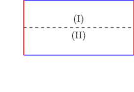
Figure 1: The two-dimensional fermion system is located on the torus. The opposite edges are glued together. The torus is divided into the two pieces with opposite directions of external electric field.

In this section we consider interaction corrections to Hall conductivity of the two dimensional systems. We follow closely discussion of [47]. We deal with the $2+1$ D tight-binding model with the interactions between electrons. The system is assumed to be placed at the surface of torus. In the other words, the periodic boundary conditions are assumed (see Fig.1 ). The x - axis is along the circle that is placed inside the torus, while the y-axis is along the circle winding along the first circle. We suppose that $y\in(-L,L]$,and $L$ is assumed very large.

We divide the cylinder into the two pieces (Fig.1 ): (I) For $y\in[0,L]$ the coupling constant $\alpha\neq 0$, and there are interactions between electrons; (II) For $y\in(-L,0)$ the value of coupling constant $\alpha^{\prime}$ is close to zero $\alpha^{\prime}\to 0$, and the inter - electron interactions are turned off.

Magnetic field is orthogonal to the surface of the torus. Its value, however, may vary in space. Notice, that strictly speaking this setup is not realistic. It requires the presence of magnetic monopoles inside the torus. However, this does not affect the logic of our gedankenexperiment. We also assume that there may be the inhomogeneous electric potential of impurities, and the other sources of inhomogeneoity. We impose also the following constraint. The dependence of external fields (that cause the mentioned inhomogeneity) in the piece (II) of the torus repeats its dependence on coordinates inside the part (I).

We represent potential $A_{\mu}$ as the sum: $A_{\mu}=A^{(m)}_{\mu}+A^{(e)}_{\mu}$. Here $A^{(m)}_{\mu}$ is gives rise to magnetic field and to potential of impurities. $A^{(e)}_{\mu}$ corresponds to the external electric field. External electric field is weak, and uniform within each of the two mentioned above reasons. In region (I) for $y\in[0,L]$ the electric field is directed along the y-axis. Inside (II) for $y\in[-L,0]$ electric field has opposite direction. We represent the action (in Euclidean space - time) as follows

$$S = \int d\tau\sum_{{\bf x,x^{\prime}}}\Big{[}\bar{\psi}_{\bf x^{\prime}}\Big{(}i(i\partial_{\tau}-A_{3}(i\tau,{\bf x}))\delta_{\bf x,x^{\prime}}-i{\cal H}_{\bf x,x^{\prime}}\Big{)}\psi_{\bf x}{-}$$ (27)

$$\alpha\bar{\psi}(\tau,{\bf x})\psi(\tau,{\bf x})\theta(y)V({\bf x-x^{\prime}})\theta(y^{\prime})\bar{\psi}(\tau,{\bf x^{\prime}})\psi(\tau,{\bf x^{\prime}})\Big{]}$$

Matrix ${\cal H}_{\bf x,x^{\prime}}$ represents the one - particle Hamiltonian in the absence of interactions. $V$ is the interaction potential. We assume the instantaneous interactions. But the case when delay is present does not give anything new. For the particular case of Coulomb interactions it receives the form $V({\bf x})=1/|{\bf x}|=1/\sqrt{x_{1}^{2}+x_{2}^{2}}$, for ${\bf x}\not={\bf 0}$.

Inside region (I) sufficiently far from the boundary with region (II) the momentum space action may be written in the form:

$$S=\int dp\bar{\psi}_{p}\hat{Q}(p,i\partial_{p})\psi_{p}{-}\alpha\int dpdqdk\bar{\psi}_{p+q}\psi_{p}\tilde{V}({\bf q})\bar{\psi}_{k}\psi_{q+k},$$

where $\hat{Q}(p,i\partial_{p})$ is Dirac operator of the given non - homogeneous system [63], while $\tilde{V}({\bf q})$ is the Fourier transform of the interaction potential. Fermion propagator with interaction corrections may be calculated as follows:

$$G_{\alpha}(x,y) = G_{0}(x,y)+\int G_{0}(x,z_{1})\Sigma(z_{1},z_{2})G_{0}(z_{2},y)dz_{1}dz_{2}+$$ (28)

$$\int G_{0}(x,z_{1})\Sigma(z_{1},z_{2})G_{0}(z_{2},z_{3})\Sigma(z_{3},z_{4})G_{0}(z_{4},y)dz_{1}dz_{2}dz_{3}dz_{4}+...$$

with $\Sigma(z_{1},z_{2})={-}\alpha G_{0}(z_{1},z_{2})\theta(y_{1})V({\bf z}_{1}-{\bf z}_{2})\theta(y_{2})+O(\alpha^{2})$, $z_{i}=({\bf z}_{i},\tau_{i})$, and $\bf z_{i}=(x_{i},y_{i})$. Next we apply Wigner transformation:

$$G_{\alpha,W}(R,p)=G_{0,W}(R,p)+G_{0,W}(R,p)\star\Sigma_{W}(R,p)\star G_{0,W}(R,p)+...,$$ (29)

In this expression $G_{0,W}(R,p)$ is solution of Groenewold equation $Q_{0,W}(R,p)\star G_{0,W}(R,p)=1$. $\Sigma_{W}$ is the Wigner transformed self - energy $\Sigma$.

V.2 Electric current expressed through the Green function with interaction corrections

Let us expand $G_{\alpha,W}(R,p)$ in powers of $\alpha$: $G_{\alpha,W}={\cal G}_{0}+\alpha{\cal G}_{1}+\alpha^{2}{\cal G}_{2}+...$ We also expand average electric current in powers of $\alpha$:

$$\bar{J}^{k}(\alpha) = {-}\int\frac{d^{2}R}{V}\int_{p}TrG_{\alpha,W}(R,p)\star\frac{\partial}{\partial p_{k}}Q_{0,W}(R,p)$$ (30)

$$= {-}\int\frac{d^{2}R}{V}\int_{p}Tr\sum_{n=0}^{\infty}G_{0,W}(\star\Sigma_{W}\star G_{0,W})^{n}\star\frac{\partial}{\partial p_{k}}Q_{0,W}(R,p)$$

Here we denote by $R$ the spatial components of coordinates. The dependence on imaginary time $\tau$ is absent in our expressions. Therefore, variable $x=(R,\tau)$ is reduced to $R$. Besides, we denote

$$\int_{p}=\int\frac{d^{3}p}{(2\pi)^{3}}$$

Correspondingly, $\Sigma_{W}=\alpha\Sigma_{1,W}+\alpha^{2}\Sigma_{2,W}+...$ and $\bar{J}^{\mu}=\bar{J}^{\mu}_{0}+\alpha\bar{J}^{\mu}_{1}+\alpha^{2}\bar{J}^{\mu}_{2}+...$, where

$$\bar{J}^{k}_{0}=\int\frac{d^{2}R}{V}\int_{p}TrG_{0,W}\star\frac{\partial}{\partial p_{k}}Q_{0,W}$$

Let us define the following quantity that is obtained when in the expression for the average current $\partial_{p_{k}}Q_{0}$ is replaced by the renormalized velocity:

$$\tilde{J}^{k}(\alpha)={-}\int\frac{d^{2}R}{V}\int_{p}TrG_{\alpha,W}(R,p)\star\frac{\partial}{\partial p_{k}}Q_{\alpha,W}(R,p).$$ (31)

Here $G_{\alpha,W}(R,p)$ satisfies equation

$$G_{\alpha,W}(R,p)\star Q_{\alpha,W}(R,p)=1$$ (32)

Since Eq. (31) is a topological invariant, its value cannot be changed, at least perturbatively, if $\alpha$ is increased smoothly from zero until the given value. Therefore, we have

$$\tilde{J}_{k}(\alpha)=\bar{J}_{k}(0)$$

and

$$\bar{J}_{k}(\alpha)-\tilde{J}_{k}(\alpha)=\bar{J}_{k}(\alpha)-\bar{J}_{k}(0)$$

We come to the conclusion that $\tilde{J}_{k}(\alpha)=\bar{J}_{k}(\alpha)$ (i.e. the electric current may be calculated using renormalized velocity $\frac{\partial}{\partial p_{k}}Q_{\alpha,W}(R,p)$) if there are no perturbative corrections to the total electric current. It appears that those corrections are indeed absent.

V.3 Non - renormalization of Hall conductance by interactions

V.3.1 First order

Electric current without interactions may be calculated as

$$\bar{J}^{k}_{0}={-}\int\frac{d^{2}R}{V}\int_{p}TrG_{0,W}(R,p)\star\frac{\partial}{\partial p_{k}}Q_{0,W}(R,p)$$

In [47] the proof is given that this expression does not receive corrections from interactions. In the first order we obtain:

$$\bar{J}^{k}_{1} = {+}\int\frac{d^{2}R}{V}\int_{p,q}Tr\Big{(}G_{0,W}(R,p-q)D_{W}(R,q)\Big{)}\frac{\partial}{\partial p_{k}}G_{0,W}(R,p)$$ (33)

where $D_{W}$ is Wigner transform of

$$D(z_{1},z_{2}) = {-}\alpha\theta(y_{1})V({\bf z}_{1}-{\bf z}_{2})\theta(y_{2}),$$ (34)

Using integration by parts we arrive at $\bar{J}_{1}^{k}=-\bar{J}^{k}_{1}$, which results in $\bar{J}_{1}^{k}=0$.

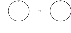
Figure 2: Example of ”Progenitor” and the corresponding self-energy diagram. This is the case of the first order correction to electric current, when there is only one progenitor diagram.

V.3.2 Second order

The second order contribution to electric current reads

$$\bar{J}^{k}_{2}={+}\int\frac{d^{2}R}{V}\int_{p}Tr\Sigma_{2,W}\star\partial_{p_{k}}G_{0,W}{+}\int\frac{d^{2}R}{V}\int_{p}Tr\Sigma_{1,W}\star G_{0,W}\star\Sigma_{1,W}\star\partial_{p_{k}}G_{0,W}$$

which in rainbow approximation is given by

$$\bar{J}^{k}_{2}\approx$$

$${+}\int\frac{d^{2}R}{V}\int_{p,k,q}\,Tr\Big{[}G_{0,W}(R,p-k)\star G_{0,W}(R,p-k-q)D_{W}(R,q)\star G_{0,W}(R,p-k)\Big{]}D_{W}(R,k)\star\partial_{p_{k}}G_{0,W}(R,p)$$

$${+}\int\frac{d^{2}R}{V}\int_{p,k,q}\,TrG_{0,W}(R,p-q)D_{W}(R,q)\star G_{0,W}(R,p)\star G_{0,W}(R,p-k)D_{W}(R,k)\star\partial_{p_{k}}G_{0,W}(R,p)$$

One can represent this result as

$$I^{k}_{2} \approx {+}\int\frac{d^{2}R}{V}\int_{p,k,q}\,Tr\Big{[}G_{0,W}(R,p-k)\star G_{0,W}(R,p-k-q)D_{W}(R,q)\star G_{0,W}(R,p-k)\Big{]}\star$$

$$\quad\quad D_{W}(R,k)\partial_{p_{k}}G_{0,W}(R,p)$$

$${+}\int\frac{d^{2}R}{V}\int_{{p,k,q}}\,TrG_{0,W}(R,p-q)D_{W}(R,q)\star G_{0,W}(R,p)\star G_{0,W}(R,p-k)D_{W}(R,k)\star\partial_{p_{k}}G_{0,W}(R,p)$$

$$= {+}\frac{1}{2}\int\frac{d^{2}R}{V}\int_{p,k,q}\,\partial_{p_{k}}\,Tr\Big{[}G_{0,W}(R,p-k)\star G_{0,W}(R,p-k-q)D_{W}(R,q)\star G_{0,W}(R,p-k)\Big{]}\star$$

$$\quad\quad D_{W}(R,k)G_{0,W}(R,p),$$

Since the last expression is the integral of total derivative, it is equal to zero. We encounter here the situation, when the diagram for the electric current is obtained from the vacuum diagram via insertion of the derivative inside the integral. The latter vacuum diagram is called ”progenitor”. The progenitor also exists in the more simple first order approximation considered above, and it is represented on the left - hand side of Fig. 2, while the corresponding contribution to electric current is represented on the right hand side of the same figure.

The two loop diagrams give

$$I^{k(cross)}_{2} = {+}\int\frac{d^{2}R}{V}\int_{p,k,q}\,Tr\Big{[}G_{0,W}(R,p-k)\circ_{2}\star G_{0,W}(R,p-k-q)\star\ _{1}\circ G_{0,W}(R,p-q)\star\partial_{p_{k}}G_{0,W}(R,p)\Big{]}$$

$$D_{W(1)}(R,k)D_{W(2)}(R,q)$$

$$= {+}\frac{1}{4}\int\frac{d^{2}R}{V}\int_{p,k,q}\partial_{p_{k}}\,Tr\Big{[}G_{0,W}(R,p-k)\circ_{2}\star G_{0,W}(R,p-k-q)\star\ _{1}\circ G_{0,W}(R,p-q)\star G_{0,W}(R,p)\Big{]}$$

$$D_{W(1)}(R,k)D_{W(2)}(R,q)$$

The last expression also vanishes. In this expression we use the following notations. Operator $\star=e^{i\overleftarrow{\partial}_{R}\overrightarrow{\partial}_{p}/2-i\overleftarrow{\partial}_{p}\overrightarrow{\partial}_{R}/2}$ acts only on $G$ and does not act on $D$, while $\circ_{i}=e^{-i\overleftarrow{\partial}_{p}\overrightarrow{\partial}_{R}/2}$ contains derivatives with respect to $p$ and $R$. The derivatives with the right arrow act on $D_{W(i)}$, while the derivatives with the left arrow act on the fermion propagator standing left to this symbol. In operator ${}_{i}\circ=e^{i\overleftarrow{\partial}_{R}\overrightarrow{\partial}_{p}/2}$ the derivatives with the right arrow act on the expression following this symbol while the derivatives with the left arrow act on $D_{W(i)}$. Notice that $D_{W(i)}$ does not contain $p$. Therefore, operator $\circ$ does not affect $G$.

This way we prove that all second order contributions to electric current vanish. The consideration of the radiative corrections of arbitrary order is, in principle, similar, but more involved. The complete proof that those contributions vanish is given in [49].

VI Application of Wigner - Weyl calculus to the QHE in non - homogeneous systems out of equilibrium

In [52] the approach of [113, 114, 115, 116, 117] to the incorporation of Wigner - Weyl calculus to Keldysh technique has been developed further. Here we briefly summarize the obtained results. Keldysh Green function is matrix

$$\hat{G}(t,x|t^{\prime},x^{\prime})=-i\left(\begin{array}[]{cc}\langle T\Phi(t,x)\Phi^{+}(t^{\prime},x^{\prime})\rangle&-\langle\Phi^{+}(t^{\prime},x^{\prime})\Phi(t,x)\rangle\\ \langle\Phi(t,x)\Phi^{+}(t^{\prime},x^{\prime})\rangle&\langle\tilde{T}\Phi(t,x)\Phi^{+}(t^{\prime},x^{\prime})\rangle\end{array}\right).$$ (38)

In this expression the Heisenberg fermionic field operator $\Phi$ is a function of both spatial coordinates $x$ and time $t$. Symbol $T$ means the time ordering while $\tilde{T}$ is the anti - time ordering. By $\langle...\rangle$ the average with respect to the initial state is denoted.

By large latin letters we denote the $D$ dimensional space - time vectors. Operator $\bf G$ corresponding to the above introduced Green function is given by: $\hat{G}(X_{1},X_{2})=\langle X_{1}|\hat{\bf G}|X_{2}\rangle$. $\bf Q$ is an operator inverse to $\bf G$.

Matrix elements $A(X_{1},X_{2})=\langle X_{1}|\hat{A}|X_{2}\rangle$ of any operator $\hat{A}$ give rise to the Weyl symbol of $\hat{A}$:

$$A_{W}(X|P)=\int d^{D}Y\,e^{\mathrm{i}Y^{\mu}P_{\mu}}A(X+Y/2,X-Y/2),\quad\mu=0,1,...,D-1$$ (39)

Weyl symbols of $\hat{G}$ and $\hat{Q}$ obey the Groenewold equation $Q\star G=1$ with the Moyal product

$$\left(A\star B\right)_{W}(X|P)=A_{W}(X|P)\,e^{{-}\mathrm{i}(\overleftarrow{\partial}_{X^{\mu}}\overrightarrow{\partial}_{P_{\mu}}-\overleftarrow{\partial}_{P_{\mu}}\overrightarrow{\partial}_{X^{\mu}})/2}B_{W}(X|P).$$ (40)

Application of this technique to the QHE of two - dimensional systems allows to obtain following results [52]:

The DC conductivity of the two - dimensional non - interacting systems is given by

$$\sigma^{ij}={\frac{1}{4}}\int\frac{d^{{3}}P}{(2\pi)^{{3}}}\mathop{\rm tr}\nolimits\left(\gamma^{<}\partial_{P_{i}}\hat{Q}_{W}\left[\hat{G}_{W}\star\partial_{{P_{[0}}}\hat{Q}_{W}\star\partial_{{P_{j]}}}\hat{G}_{W}\right]\right)+{\rm c.c.}$$ (41)

Here trace is taken over Keldysh components as well as over the internal indices, and

$$\gamma^{<}=\left(\begin{array}[]{cc}0&0\\ 1&0\end{array}\right).$$

It was shown that the above expression for the conductivity averaged over the system area is reduced to the topological formula Eqs. (12), (13). The intermediate expression through the real - time Green functions obtained in our derivation reproduces the one of [118].

Interaction corrections to the QHE conductivity were calculated, and it was shown that already in the one loop order those corrections do not vanish in case of equilibrium at finite temperature, and also out of equilibrium.

VII Conclusions

To conclude, in this paper we review the results obtained by the group working in Ariel University. We summarize here the results reported previously in a series of papers [26, 47, 48, 49, 50, 51, 52, 53] (see also references therein to the other papers of the group). In these works the non - dissipative transport phenomena have been investigated using the technique of Wigner - Weyl calculus. The obtained results concern the chiral magnetic effect (CME), the chiral separation effect (CSE) and the quantum Hall effect (QHE). The considered systems are essentially non - homogeneous. This is why the use of the Wigner - Weyl calculus for obtaining the topological expressions seems to us inevitable.

Below we summarize the main obtained results

1. The approximate Wigner-Weyl calculus for the lattice models has been developed. It allows to deal with the systems in the presence of weak inhomogeneity. Weakness of inhomogeneity means that physical quantities almost do not vary at the distance of the order of the lattice spacing. Within this calculus we develop Wigner - Weyl field theory in equilibrium [26, 48], and its extension to quantum kinetic theory [52]. In this theory currents and conductivities are expressed through the Wigner transformed fermion propagators and Weyl symbols of operators.

2. It is shown that the CME conductivity is absent in true equilibrium both at zero and at finite temperatures [52]. Weak inhomogeneity cannot affect this conclusion. Inter - electron interactions also do not affect this conclusion, at least, in one - loop order. Notice that we did not consider here the zero frequency limit of non - equilibrium CME conductivity. The latter limit is to be the subject of a separate study and it might be different from the case of the true equilibrium, when the system is not subject to the time dependent chiral chemical potential.

3. We have shown that the radiative corrections to the QHE conductivity in the two - dimensional systems are absent. We have shown this first in the first and the second orders of perturbation theory [47], and later extended this proof to the third order and to the higher orders of perturbation theory [49]. Besides, we demonstrate that the QHE conductivity in the presence of interactions may be calculated using the same expression as the QHE conductivity of the non - interacting systems, in which the Green function is replaced by the complete interacting one.

4. The CSE is considered for the non - homogeneous systems with chiral fermions [50]. We assume that in these systems the effective low energy theory obeys chiral symmetry. On the language of Green functions it is expressed as follows: matrix $\gamma^{5}$ commutes or anti - commutes with the Wigner transformed Green function, and with the Weyl symbol of lattice Dirac operator (the latter is inverse to the Green function). This requirement is imposed on piece of phase space with any values of coordinates, but for the region of momenta that belongs to a vicinity of the Fermi surface. For such systems the CSE conductivity is given by the integral over coordinates $x$ and for each value of $x$ over the $3D$ hypersurface surrounding the analogue of the Fermi surface. The latter is understood as the points in momentum space, where expression standing in the mentioned integral has poles.

5. In the framework of Keldysh theory we consider the QHE conductivity and derive its useful representation through the Wigner transformed Keldysh propagators [52]. As it should, this representation is reduced to the topological one of [26] when the system approaches equilibrium with vanishing temperature. At the same time out of equilibrium and in thermal equilibrium with finite temperature the QHE conductivity is not robust to the smooth modification of the system. Besides, our consideration of interaction corrections demonstrates that the radiative corrections to the QHE conductivity do not vanish out of equilibrium as well as in thermal equilibrium with finite temperature.

The results reviewed in the present paper have been obtained in collaboration with C.Banerjee, I.Fialkovsky, M.Lewkowicz, M.Suleymanov, X.Wu, C.X.Zhang. The author is grateful to all former and present members of the group for this collaboration and for the important contributions to the obtained results. Besides, the author kindly acknowledges numerous discussions with G.E. Volovik and Z.V.Khaidukov.

References

- Groenewold [1946] H. J. Groenewold, On the Principles of elementary quantum mechanics, Physica 12, 405 (1946).
- Moyal [1949] J. E. Moyal, Quantum mechanics as a statistical theory, in Proceedings of the Philosophical Society, 45 (1949) pp. 99–124.
- Weyl [1927] H. Weyl, Quantenmechanik und Gruppentheorie, Zeitschrift fur Physik 46, 1 (1927).
- Wigner [1932] E. P. Wigner, On the quantum correction for thermodynamic equilibrium, Phys. Rev 40, 749 (1932).
- Ali and Englis [2005] S. T. Ali and M. Englis, Quantization Methods: A Guide for Physicists and Analysts, Rev. Math. Phys. 17, 391 (2005).
- Berezin and Shubin [1972] F. A. Berezin and M. A. Shubin, in: Colloquia Mathematica Societatis Janos Bolyai (North-Holland Amsterdam), , 21 (1972).
- Curtright and Zachos [2012] T. L. Curtright and C. K. Zachos, Quantum Mechanics in Phase Space, Asia Pacific Physics Newsletter 1, 37 (2012), arXiv:1104.5269 .
- Zachos et al. [2005] C. Zachos, D. Fairlie, and T. Curtright, Quantum Mechanics in Phase Space (World Scientific, Singapore, 2005).
- Cohen [1966] L. Cohen, Generalized phase-space distribution functions, Journal of Mathematical Physics 7, 781 (1966).
- Agarwal and Wolf [1970] G. S. Agarwal and E. Wolf, Calculus for functions of noncommuting operators and general phase-space methods in quantum mechanics. i. mapping theorems and ordering of functions of noncommuting operators, Phys. Rev. D 2, 2161 (1970).
- G. [1963] E. C. G., Sudarshan Equivalence of Semiclassical and Quantum Mechanical Descriptions of Statistical Light Beams, Phys. Rev. Lett. 10, 277 (1963).
- Glauber [1963] R. J. Glauber, Coherent and Incoherent States of the Radiation Field, Phys. Rev 131, 2766 (1963).
- Husimi [1940] K. Husimi, Some formal properties of the density matrix, in Proc. Phys. Math. Soc. Jpn. 22 (1940) pp. 264–314.
- Cahill and J. [1969] K. E. Cahill and R. J., Glauber ordered expansions in boson amplitude operators, Phys. Rev. 177, 1882 (1969).
- Buot [2009] F. A. Buot, Nonequilibrium Quantum Transport Physics in Nanosystems (World Scientific, 2009).
- Lorce and Pasquini [2011] C. Lorce and B. Pasquini, Quark Wigner distributions and orbital angular momentum, Phys.Rev. D 84, 014015 (2011), arXiv:1106.0139 .
- Elze et al. [1986] H. T. Elze, M. Gyulassy, and D. Vasak, Transport equations for the QCD Quark Wigner Operator, Nucl. Phys. B 706, 276 (1986).
- Hebenstreit et al. [2010] F. Hebenstreit, R. Alkofer, and H. Gies, Schwinger pair production in space and time-dependent electric fields: relating the Wigner formalism to quantum kinetic theory, Phys. Rev. D 82, 105026 (2010), arXiv:1007.1099 .
- Calzetta et al. [1988] E. Calzetta, S. Habib, and B. L. Hu, Quantum Kinetic Field Theory in curved space-time: covariant Wigner function and Liouville-Vlasov equation, Phys. Rev. D 37, 2901 (1988).
- Buot [1974] F. A. Buot, Method for calculating in solid-state theory, Phys.Rev. B 10, 3700 (1974).
- Buot [2013] F. A. Buot, Quantum Superfield Theory and Lattice Weyl Transform in Nonequilibrium Quantum Transport Physics, Quantum Matter 2, 247 (2013).
- Wootters [1987] W. K. Wootters, A wigner-function formulation of finite-state quantum mechanics, Annals of Physics 176, 1 (1987).
- Leonhardt [1995] U. Leonhardt, Quantum-state tomography and discrete wigner function, Phys. Rev. Lett. 74, 4101 (1995).
- Kasperkovitz and Peev [1994] P. Kasperkovitz and M. Peev, Wigner-weyl formalisms for toroidal geometries, Annals of Physics 230, 21 (1994).
- Ligabò [2016] M. Ligabò, Torus as phase space: Weyl quantization, dequantization, and wigner formalism, Journal of Mathematical Physics 57, 082110 (2016).
- Zubkov and Wu [2019] M. A. Zubkov and X. Wu, Topological invariant in terms of the Green functions for the Quantum Hall Effect in the presence of varying magnetic field (2019), arXiv:arXiv:1901.06661 [cond-mat.mes-hall] .
- Zubkov and Khaidukov [2017] M. A. Zubkov and Z. V. Khaidukov, Topology of the momentum space, Wigner transformations, and a chiral anomaly in lattice models, JETP Lett. 106, 166 (2017), [Pisma Zh. Eksp. Teor. Fiz. 106 no.3, 166].
- Chernodub and Zubkov [2017] M. N. Chernodub and M. A. Zubkov, Scale magnetic effect in Quantum Electrodynamics and the Wigner-Weyl formalism, Phys. Rev. D 96, 056006 (2017), arXiv:1703.06516 .
- Khaidukov and Zubkov [2017] Z. V. Khaidukov and M. A. Zubkov, Chiral Separation Effect in lattice regularization, Phys. Rev. D 95, 074502 (2017), arXiv:1701.03368 .
- Zubkov [2018] M. A. Zubkov, Momentum space topology of QCD, Annals Phys 393, 264 (2018), arXiv:1610.08041 .
- Zubkov [2016a] M. A. Zubkov, Absence of equilibrium chiral magnetic effect, Phys. Rev. D 93, 105036 (2016a), arXiv:1605.08724 .
- Zubkov [2016b] M. A. Zubkov, Wigner transformation, momentum space topology, and anomalous transport, Annals Phys 373, 298 (2016b), arXiv:1603.03665 .
- Chernodub [2016] M. N. Chernodub, Anomalous transport due to the conformal anomaly, Phys. Rev. Lett 117, 141601 (2016), arXiv:1603.07993 .
- Volovik [2003] G. E. Volovik, The Universe in a Helium Droplet (Clarendon Press, Oxford, 2003).
- Matsuyama [1987] T. Matsuyama, Quantization of Conductivity Induced by Topological Structure of Energy Momentum Space in Generalized QED in Three-dimensions, Prog. Theor. Phys 77, 711 (1987).
- Thouless et al. [1982] D. J. Thouless, M. Kohmoto, M. P. Nightingale, and M. den Nijs, Quantized Hall Conductance in a Two-Dimensional Periodic Potential, Phys. Rev. Lett. 49, 405 (1982).
- Avron et al. [1983] J. E. Avron, R. Seiler, and B. Simon, Homotopy and quantization in condensed matter physics, Phys. Rev. Lett. 51, 51 (1983).
- Fradkin [1991] E. Fradkin, Field Theories of Condensed Matter Physics (Addison Wesley Publishing Company, 1991).
- Tong [2016] D. Tong, Lectures on the quantum hall effect (2016), arXiv:1606.06687 [hep-th] .
- Hatsugai [1997] Y. Hatsugai, Topological aspects of the quantum Hall effect, J. Phys. Condens. Matter 9, 2507 (1997).
- Qi et al. [2008] X.-L. Qi, T. L. Hughes, and S.-C. Zhang, Topological field theory of time-reversal invariant insulators, Phys. Rev. B 78, 195424 (2008).
- Ishikawa and Matsuyama [1986] K. Ishikawa and T. Matsuyama, Magnetic field induced multi component QED in three-dimensions and quantum Hall effect, Z. Phys. C 33, 41 (1986).
- Volovik [1988] G. E. Volovik, An analog of the quantum Hall effect in a superfluid 3He film, JETP 67, 9 (1988), zhETF, Vol. 94, No. 3(9), 123.
- Coleman and Hill [1985] S. Coleman and B. Hill, Phys. Lett. B 159, 184 (1985).
- Lee [1986] T. Lee, Phys. Lett. B 171, 247 (1986).
- Zhang and Zubkov [2019a] C. X. Zhang and M. A. Zubkov, Influence of interactions on the anomalous quantum Hall effect (2019a), arXiv:arXiv:1902.06545 [cond-mat.mes-hall] .
- Zhang and Zubkov [2019b] C. X. Zhang and M. A. Zubkov, Hall conductivity as the topological invariant in phase space in the presence of interactions and non-uniform magnetic field, JETP letters (2019b), arXiv:arXiv:1908.04138 .
- Fialkovsky et al. [2020] I. V. Fialkovsky, M. Suleymanov, X. Wu, C. X. Zhang, and M. A. Zubkov, Hall conductivity as topological invariant in phase space, Physica Scripta 95, 064003 (2020).
- Zhang and Zubkov [2021] C. X. Zhang and M. A. Zubkov, Influence of interactions on integer quantum hall effect (2021), arXiv:2011.04030 [cond-mat.mes-hall] .
- Suleymanov and Zubkov [2020] M. Suleymanov and M. Zubkov, Chiral separation effect in nonhomogeneous systems, Physical Review D 102, 10.1103/physrevd.102.076019 (2020).
- Banerjee et al. [2021a] C. Banerjee, M. Lewkowicz, and M. A. Zubkov, Equilibrium chiral magnetic effect: Spatial inhomogeneity, finite temperature, interactions, Physics Letters B 819, 136457 (2021a).
- Banerjee et al. [2021b] C. Banerjee, I. V. Fialkovsky, M. Lewkowicz, et al., Wigner-weyl calculus in keldysh technique, J Comput Electron 20, 2255 (2021b).
- Zhang and Zubkov [2019c] C. X. Zhang and M. A. Zubkov, Feynman Rules in terms of the Wigner transformed Green’s functions, preprint ([hep-ph]. Phys.Lett.B (2020), 2019) arXiv:1911.11074 .
- Vilenkin [1980] A. Vilenkin, Phys, Rev. D 22, 3080 (1980).
- [55] .
- Kharzeev [2014] D. E. Kharzeev, The chiral magnetic effect and anomaly-induced transport, Prog. Part 75, 10.1016/j.ppnp.2014.01.002 (2014), arXiv:1312.3348 .
- Kharzeev and Warringa [2009] D. E. Kharzeev and H. J. Warringa, Chiral magnetic conductivity, Phys. Rev 80, 10.1103/PhysRevD.80.034028 (2009), arXiv:0907.5007 .
- [58] D. T. Son and N. Yamamoto, ”berry curvature, triangle anomalies, and chiral magnetic effect in fermi liquids”, Phys.Rev.Lett. 109, 18160, arXiv:1203.2697 .
- [59] S. N. Valgushev, M. Puhr, and P. V. Buividovich, Chiral Magnetic Effect in finite-size samples of parity-breaking Weyl semimetals ([cond-mat.str-el]) arXiv:1512.01405 .
- Buividovich et al. [2015] P. V. Buividovich, M. Puhr, and S. N. Valgushev, Chiral magnetic conductivity in an interacting lattice model of parity-breaking weyl semimetal, Phys. Rev 92, 10.1103/PhysRevB.92.205122 (2015), arXiv:1505.04582 .
- Buividovich [2014a] P. V. Buividovich, Spontaneous chiral symmetry breaking and the chiral magnetic effect for interacting dirac fermions with chiral imbalance, Phys. Rev 90, 10.1103/PhysRevD.90.125025 (2014a), arXiv:1408.4573 .
- Buividovich [2014b] P. V. Buividovich, Anomalous transport with overlap fermions, Nucl. Phys 925, 10.1016/j.nuclphysa.2014.02.022 (2014b), arXiv:1312.1843 .
- Zubkov [2016c] M. A. Zubkov, “wigner transformation, momentum space topology, and anomalous transport,”, Annals Phys 373 (2016c), arXiv:1603.03665 .
- Zubkov [2016d] M. A. Zubkov, “absence of equilibrium chiral magnetic effect,”, Phys. Rev 93 (2016d), arXiv:1605.08724 .
- Vazifeh and Franz [2013] M. M. Vazifeh and M. Franz, Phys, Rev. Lett. 111, 027201 (2013).
- Yamamoto [2015] N. Yamamoto, Phys, Rev. D 92, 085011 (2015).
- Nielsen and Ninomiya [1983] H. B. Nielsen and M. Ninomiya, Adler-bell-jackiw anomaly and weyl fermions in crystal, Phys. Lett. B 130, 389 (1983).
- [68] Q. Li, D. E. Kharzeev, C. Zhang, Y. Huang, I. Pletikosic, A. V. Fedorov, R. D. Zhong, J. A. Schneeloch, G. D. Gu, and T. Valla, arXiv:1412.6543 .
- Wu and and [2017] Y. Wu and D. H. and, and h. c, Ren, Phys 96, 10.1103/PhysRevD.96.096015 (2017), arXiv:1601.06520 .
- [70] M. A. Metlitski and A. R. Zhitnitsky, Anomalous axion interactions and topological currents in dense matter, Phys. Rev. D 72, 045011.
- [71] D. E. Kharzeev, J. Liao, S. A. Voloshin, and G. Wang, Chiral Magnetic Effect in High-Energy Nuclear Collisions — A Status Report ([hep-ph]) arXiv:1511.04050 .
- Kharzeev [2009] D. E. Kharzeev, Chern-simons current and local parity violation in hot qcd matter, Nucl. Phys 830, 10.1016/j.nuclphysa.2009.10.049 (2009), arXiv:0908.0314 .
- Csernai et al. [2016] L. P. Csernai, V. K. Magas, and D. J. Wang, Flow vorticity in peripheral high energy heavy ion collisions, Phys. Rev 87 (2016), arXiv:1302.5310 .
- Fukushima and Hatsuda [2011] K. Fukushima and T. Hatsuda, The phase diagram of dense qcd, Rept. Prog. Phys 74, 10.1088/0034-4885/74/1/014001 (2011), arXiv:1005.4814 .
- Smilga [1997] A. V. Smilga, “physics of thermal qcd,” phys, Rept. 291, 1 (1997), arXiv:hep-ph/9612347 .
- [76] K. Rajagopal and F. Wilczek, “The condensed matter physics of QCD (”) arXiv:hep-ph/0011333 .
- Rischke [2004] D. H. Rischke, “the quark-gluon plasma in equilibrium,” prog, Part 52, 197 (2004), arXiv:nucl-th/0305030 .
- Alford et al. [2008] M. G. Alford, A. Schmitt, K. Rajagopal, and T. Schafer, “color superconductivity in dense quark matter,” rev, Mod. Phys 80, 1455 (2008), arXiv:0709.4635 .
- [79] R. S. Hayano and T. Hatsuda, “hadron properties in the nuclear medium,” [nucl-ex]. [17] h, Satz, “The states of matter in QCD,” arXiv:0 903, 2778, arXiv:0812.1702 .
- [80] M. Huang, “qcd phase diagram at high temperature and density,” [hep-ph]. [19] a, Schmitt, “Dense matter in compact stars - A pedagogical introduction,” arXiv: 1001, 3294, arXiv:1001.3216 .
- Andersen et al. [2016] J. O. Andersen, W. R. Naylor, and A. Tranberg, Phase diagram of qcd in a magnetic field: A review, Rev. Mod 88 (2016), arXiv:1411.7176 .
- Fukushima and Sasaki [2013] K. Fukushima and C. Sasaki, The phase diagram of nuclear and quark matter at high baryon density, Prog. Part 72 (2013), arXiv:1301.6377 .
- Miransky and Shovkovy [2015] V. A. Miransky and I. A. Shovkovy, Quantum field theory in a magnetic field: From quantum chromodynamics to graphene and dirac semimetals, Phys. Rept. 576 (2015), arXiv:1503.00732 .
- Zhitnitsky [2013] A. R. Zhitnitsky, Qcd as a topologically ordered system, Annals Phys 336 (2013), arXiv:1301.7072 .
- Zyuzin and Burkov [2012] A. A. Zyuzin and A. A. Burkov, Topological response in Weyl semimetals and the chiral anomaly, Phys. Rev. B 86, 115133 (2012), arXiv:1206.1868 .
- Gorbar et al. [2015] E. V. Gorbar, V. A. Miransky, I. A. Shovkovy, and P. O. Sukhachov, Chiral separation and chiral magnetic effects in a slab: The role of boundaries, Phys. Rev 92, 10.1103/PhysRevB.92.245440 (2015), arXiv:1509.06769 .
- [87] Z. V. Khaidukov and M. A. Zubkov, Chiral separation effect in lattice regularization, Phys. Rev. D 2017, 10.1103/PhysRevD.95.074502.
- [88] E. V. Gorbar et al., “Radiative Corrections to Chiral Separation Effect in QED.” Physical Review D 88.2 (2013): n. pag (Crossref. Web).
- Keldysh and Eksp [1965] L. V. Keldysh and Z. Eksp, Teor, Fiz. 47 (1965).
- Bonitz [2000] M. Bonitz, ed., Progress in Nonequilibrium Green’s Functions (World Scientific, Singapore, 2000).
- Bonitz and Semkat [2003] M. Bonitz and D. Semkat, eds., Progress in Nonequilibrium Green’s Functions II (World Scientific, Singapore, 2003).
- Bonitz and Filinov [2006] M. Bonitz and A. Filinov, eds., Progress in Nonequilibrium Green’s Functions III (Conference Series 35, Journal of Physics, 2006).
- Kadanoff and Baym [1962] L. P. Kadanoff and G. Baym, Quantum Statistical Mechanics (Benjamin, New York, 1962).
- Baym [1962] G. Baym, Phys, Rev. 127, 1391 (1962).
- [95] J. Schwinger and J. Math, Phys. 2 (1961), 407.
- Matsubara [1955] T. Matsubara, Prog, Theor. Phys 14, 351 (1955).
- Bloch and de Donimicis [1959] C. Bloch and C. de Donimicis, Nucl, Phys. 10, 509 (1959).
- Gaudin [1960] M. Gaudin, Nucl, Phys. 15, 89 (1960).
- Abrikosov et al. [1963] A. A. Abrikosov, L. P. Gor’kov, and I. E. Dzyaloshinski, Methods of Quantum Field Theory in Statistical Physics (Prentice-Hall, Englewood Cliffs, N.J, 1963).
- Kamenev [2011] A. Kamenev, Field theory of non-equilibrium systems, by alex kamenev, cambridge, uk: Cambridge university press, 2011 (2011).
- Langreth [1976] D. C. Langreth, in, in Linear and Nonlinear Electron Transport in Solids (J. T. Devreese and V. E. van Doren (Plenum Press, New York p. 3, 1976).
- Rammer [2007] J. Rammer, Quantum Field Theory of Nonequilibrium States (Cambridge University Press, Cambridge, 2007).
- Landau and Eksp [1957] L. D. Landau and Z. Eksp, Teor, Fiz. 30 (1957).
- Luttinger and Ward [1960] J. M. Luttinger and J. C. Ward, Phys, Rev. 118, 1417 (1960).
- Luttinger [1960] J. M. Luttinger, Phys, Rev. 119, 1153 (1960).
- Caroli et al. [1971] C. Caroli, R. Combescot, P. Nozières, and J. o. P. D. Saint-James, C: Solid st, Phys. 4, 916 (1971).
- Aronov and Gurevich [1975] A. G. Aronov and V. L. Gurevich, Fiz, Tverd. Tela 16 (1975).
- Larkin and Ovchinnikov [1975] A. I. Larkin and Y. B. Ovchinnikov, Zh, Eksp. Teor. Fiz. 68 (1975).
- [109] P. Danielewicz, Ann. of phys. 152 (1984), 239.
- Chou et al. [1985] K. C. Chou, Z. B. Su, B. L. Hao, and L. Yu, Phys, Rep. 118, 1 (1985).
- Rammer and Smith [1986] J. Rammer and H. Smith, Rev, Mod. Phys 58, 323 (1986).
- Iancu et al. [2001] E. Iancu, A. Leonidov, and L. D. McLerran, Nucl, Phys.A 692, 583 (2001).
- [113] A. Shitade, Anomalous Thermal Hall Effect in a Disordered Weyl Ferromagnet. Journal of the Physical Society of Japan 86.5 (2017): 054601 (Crossref. Web).
- Onoda et al. [2006a] S. Onoda, N. Sugimoto, and N. Nagaosa, Prog, Theor.Phys. 116, 61 (2006a).
- Onoda et al. [2006b] S. Onoda, N. Sugimoto, and N. Nagaosa, Phys, Rev. Lett. 97, 2 (2006b).
- Sugimoto et al. [2007] N. Sugimoto, S. Onoda, and N. Nagaosa, Prog, Theor.Phys. 117, 415 (2007).
- Onoda et al. [2008] S. Onoda, N. Sugimoto, and N. Nagaosa, Phys, Rev. B 77, 3 (2008).
- Lux et al. [a] F. R. Lux, F. Freimuth, S. Blegel, and Y. Mokrousov, Chiral hall effect in noncollinear magnets from a cyclic cohomology approach, Physical Review Letters 124, 096602 (a).
- Lux et al. [b] F. R. Lux, P. Prass, S. Blgel, and Y. Mokrousov, Effective seiberg-witten gauge theory of noncollinear magnetism, arxiv, arXiv:2005.12629 (b), preprint.
- Zubkov [2016e] M. A. Zubkov, Phys, Rev.D 93, 10 (2016e).