Gap Minimization for Knowledge Sharing and Transfer

Abstract

Learning from multiple related tasks by knowledge sharing and transfer has become increasingly relevant over the last two decades. In order to successfully transfer information from one task to another, it is critical to understand the similarities and differences between the domains. In this paper, we introduce the notion of performance gap, an intuitive and novel measure of the distance between learning tasks. Unlike existing measures which are used as tools to bound the difference of expected risks between tasks (e.g., $\mathcal{H}$-divergence or discrepancy distance), we theoretically show that the performance gap can be viewed as a data- and algorithm-dependent regularizer, which controls the model complexity and leads to finer guarantees. More importantly, it also provides new insights and motivates a novel principle for designing strategies for knowledge sharing and transfer: gap minimization. We instantiate this principle with two algorithms: 1. $\operatorname{\mathsf{gapBoost}}$, a novel and principled boosting algorithm that explicitly minimizes the performance gap between source and target domains for transfer learning; and 2. $\operatorname{\mathsf{gapMTNN}}$, a representation learning algorithm that reformulates gap minimization as semantic conditional matching for multitask learning. Our extensive evaluation on both transfer learning and multitask learning benchmark data sets shows that our methods outperform existing baselines.

Keywords: Performance Gap, Transfer Learning, Multitask Learning, Regularization, Algorithmic Stability

1 Introduction

Transfer and multitask learning have been extensively studied over the last two decades (Pan and Yang, 2010; Weiss et al., 2016). In both learning paradigms, the underlying assumption is that there is common knowledge that can be transferred or shared across different tasks. This sharing of knowledge can lead to a better generalization performance than learning each task individually. In particular, transfer learning improves the learning performance on a target domain by leveraging knowledge from different (but related) source domains, while multitask learning simultaneously learns multiple related tasks to improve the overall performance. However, not all tasks are equally related, and therefore sharing some information may be more beneficial than sharing other. In this work, we investigate how to quantify the similarity between tasks in a manner that is conducive to better knowledge-sharing algorithms. While the two paradigms of transfer and multitask learning are conceptually intertwined, they have typically been studied separately. From the theoretical aspect, most existing results on transfer learning primarily focus on domain adaptation (Ganin et al., 2016), where no label information is available in the target domain. As a result, the benefits of transfer learning when target labels are available have remained elusive, and existing generalization bounds require additional assumptions for domain adaptation to succeed, which cannot be accurately estimated due to the lack of labeled examples in the target domain (e.g., the labeling function is $\lambda$-close to the hypothesis class (Ben-David et al., 2007, 2010)). Similarly, for multitask learning, most existing methods and theoretical results only consider aligning marginal distributions to learn task-invariant feature representations (Maurer et al., 2016; Luo et al., 2017a) or task relations (Zhang and Yeung, 2012; Bingel and Søgaard, 2017; Shui et al., 2019; Zhou et al., 2021c), without taking advantage of label information of the tasks. Consequently, the features can lack discriminative power for supervised learning even if their marginal distributions have been properly matched.

In this paper, the fundamental question we address is: when label information is available, how can we leverage it to measure the distance between tasks and to motivate concrete algorithms that share and transfer knowledge between the tasks? To this end, we develop a unified theoretical framework for transfer learning and multitask learning by introducing the notion of performance gap, an intuitive and novel measure of the divergence between different learning tasks. Intuitively, if the learning tasks are similar to each other, the model trained on one task should also perform well on the other tasks, and vice versa. We formalize this intuition by showing that the transfer and multitask learning model complexities (and consequently their generalization errors) can be upper-bounded in terms of the performance gap. Our formulation eventually leads to gap minimization, a general principle that is applicable to a large variety of forms of knowledge sharing and transfer, and provides a deeper understanding of this problem and new insight into how to leverage the labeled data instances. Gap minimization is, to the best of our knowledge, the first unified principle that accommodates both transfer and multitask learning with the presence of labeled data. On the other hand, the specific form that gap minimization takes depends on the underlying transfer or multitask learning approach, and therefore the performance gap can be viewed as a data- and algorithm-dependent regularizer, which leads to finer and more informative generalization bounds. On the algorithmic side, the gap minimization principle also motivates new strategies for knowledge sharing and transfer.

Our analysis is based on algorithmic stability (Bousquet and Elisseeff, 2002). Most existing theoretical justifications for transfer and multitask learning in the literature based on algorithmic stability have examined the convergence rate of the stability coefficient under the assumption that the model complexity (and hence the loss function) of an algorithm is upper-bounded by a fixed constant. However, as we demonstrate in this work, the model complexity itself can be viewed as a function of the performance gap, which lends a new perspective on transfer and multitask learning algorithms. In particular, we show in a diversity of settings that a small performance gap equates to a small model complexity. This provides mathematical evidence for the intuition that if two tasks are similar to each other, transfer or multitask learning across these two tasks can successfully improve model performance. Usefully, in many cases, this performance gap is modulated by algorithm parameters (e.g., instance weights or representational parameters) and can therefore be minimized. In some settings, our analysis does not reveal immediate gap minimization strategies; in such cases, our analysis still provides theoretical insights that reveal when knowledge sharing and transfer can successfully improve performance.

We instantiate the principle of gap minimization with three algorithms: $\operatorname{\mathsf{gapBoost}}$ for transfer learning in classification problems, $\operatorname{\mathsf{gapBoostR}}$ for transfer learning in regression problems, and $\operatorname{\mathsf{gapMTNN}}$ for deep multitask learning. $\operatorname{\mathsf{gapBoost}}$ and $\operatorname{\mathsf{gapBoostR}}$ are based on four rules derived from our generalization bounds that explicitly minimize the performance gap between source and target domains. As boosting algorithms, they offer out-of-the-box usability and readily accommodate any base algorithm for transfer learning. To make gap minimization feasible in a deep learning setting, we create $\operatorname{\mathsf{gapMTNN}}$ by reformulating the gap minimization problem as semantic conditional matching. In addition, we also derive a theoretical analysis on representation learning based on the notion of conditional Wasserstein distance (Arjovsky et al., 2017; Shui et al., 2021), which justifies our algorithm and motivates practical guidelines in the deep learning regime.

The remainder of this paper is organized as follows. Section 2 provides a brief overview of related work. Section 3 presents the preliminaries and notions used for our analysis. Our main theoretical results are presented in Section 4, followed by $\operatorname{\mathsf{gapBoost}}$ and $\operatorname{\mathsf{gapMTNN}}$ described in Section 5. The experimental results are reported in Section 6. Section 7 presents our conclusions and avenues for future work.

An earlier version of some of the results in this paper appeared in the International Conference on Artificial Intelligence and Statistics (Wang et al., 2019b) and in Advances in Neural Information Processing Systems (Wang et al., 2019a). This submission substantially extends those results, containing: (1) extension of prior theoretical results to other transfer and multitask learning scenarios in Sections 4.1.2, 4.1.3, 4.2.1, and 4.2.3; (2) $\operatorname{\mathsf{gapBoostR}}$, a novel transfer boosting algorithm for regression problems in Section 5.1; (3) $\operatorname{\mathsf{gapMTNN}}$, a novel multitask representation learning algorithm in Section 5.2; and (4) additional experiments on transfer regression multitask learning problems in Sections 6.1.1 and 6.2. More importantly, in addition to the theoretical results and algorithms developed for two specific learning scenarios in our previous works, this paper presents a comprehensive and unified framework for both transfer and multitask learning based on the notion of performance gap, which opens up avenues for future work.

2 Related Work

A large number of theoretical analyses on transfer learning and multitask learning have been developed. Thus, we briefly review the most related work.

2.1 Transfer learning

Most results in transfer learning have been obtained for the domain adaptation setting, where label information in the target domain is generally not available (Pan and Yang, 2010; Wilson and Cook, 2020). To deal with the lack of label information in the target domain, multiple works have used the $\mathcal{H}$-divergence to measure the distance between two domains in terms of the data distribution in the feature space for binary classification (Ben-David et al., 2007; Blitzer et al., 2008; Ben-David et al., 2010). This theory was later extended to the general loss function by introducing the discrepancy distance (Mansour et al., 2009), Wasserstein distance (Redko et al., 2017), and Jensen-Shannon divergence (Shui et al., 2022b).

For transfer learning based on instance weighting, the concept of distributional stability was introduced by (Cortes et al., 2008) to analyze the generalization gap between the perfect weighting scheme and the kernel mean matching (KMM) (Huang et al., 2007). Other works in this setting studied a transfer learning algorithm that minimizes a convex combination of the empirical risks of the source and target domains (Blitzer et al., 2008; Ben-David et al., 2010). In the context of representation learning, theoretical results focus on learning transferable representations (Liang et al., 2020). For instance, (Zhang et al., 2019) proposed a domain adaptation margin theory based on the hypothesis-induced discrepancy. The importance of task diversity was studied by (Tripuraneni et al., 2020), who obtained statistical guarantees for transfer learning by studying the impact of representation learning for transfer learning. Another approach adopted a Bayesian perspective of causal theory induction and used these theories to transfer knowledge between different environments (Edmonds et al., 2020). In addition, it has been revealed that the function of the source domain data can be interpreted as a regularization matrix which benefits the learning process of the target domain task (Liu et al., 2017c). However, as the proof schema in this latter work does not exploit the label information in the source domain, the generalization bound does not verify the benefits of source data. On the other hand, the fundamental limits of unsupervised domain adaptation have been investigated, showing that there is no guarantee for successful domain adaptation if label information is not available (Zhao et al., 2019).

When target label information is available, several transfer learning algorithms with theoretical justifications have been proposed. A boosting approach was proposed to reweight the data from different domains (Dai et al., 2007; Wang and Pineau, 2015). While the effectiveness of the algorithm has been empirically verified, the theoretical analysis based on VC-dimension did not demonstrate the benefit of transferred knowledge. Other work proved the benefits of sparse coding by showing that by embedding the knowledge from the source domains into a low-dimensional dictionary, the resulting model had smaller Rademacher complexity (Maurer et al., 2013). In the setting of hypothesis transfer, analysis of the algorithmic stability has shown that good prior knowledge learned from source domains guarantees not only good generalization, but also fast recovery of the performance of the best hypothesis in the class (Kuzborskij and Orabona, 2013, 2017). More recent work has focused on the setting where limited target labels are available. For example, (Mansour et al., 2021) developed a novel meta-learning theory when learning limited target labels in the presence of multiple sources. Another approach for semi-supervised domain adaptation used entropy minimization (Saito et al., 2019). A novel, theoretically justified method for semi-supervised domain adaptation has recently been proposed for using min-max to align the marginal and conditional distributions between source and target domains (Li et al., 2021). (Acuna et al., 2020) obtained a generalization bound based on the $f$-divergences of different distributions. Other recent work studied minimax lower bounds to characterize the fundamental limits of transfer learning in the context of regression (Kalan et al., 2020).

2.2 Multitask learning

There have also been extensive theoretical studies on multitask learning. For example, by utilizing the notations of VC-dimension and covering number, the generalization bound of multitask learning has been investigated under the assumption that the tasks share some common hypothesis space (Baxter, 2000). Later, improved bounds were presented under the assumption that the tasks are related in a way such that they share a common linear operator which is chosen to preprocess data (Maurer, 2006), or the linear model parameters lie in a low-dimensional subspace (Maurer et al., 2013, 2016). The latter work was also extended to eigenvalue decomposition (Wang et al., 2016) and nonlinear model by gradient boosting (Wang and Pineau, 2016). More recently, algorithm-dependent bounds have also been analyzed, based on the notation of algorithmic stability (Zhang, 2015; Liu et al., 2017b). Moreover, it has also been proved that the algorithmic stability method has the potential to derive tighter generalization upper bounds than the approaches based on the VC-dimension and Rademacher complexity (Liu et al., 2017b). Other work used random matrix theory to analyze the performance of the multitask least-square SVM algorithm (Tiomoko et al., 2020). (Zhang et al., 2020) studied generalization bounds from the perspective of vector-valued function learning, specifically analyzing under what conditions multitask learning can perform better than single-task learning.

In the context of representation learning, (Chen et al., 2018) proposed a method to balance the joint training of multiple tasks to ensure that all tasks are trained at approximately the same rate. (Shui et al., 2019) explored a generalization bound that combines task similarity together with representation learning under an adversarial training scheme (Ben-David et al., 2010; Shen et al., 2018). In the setting of deep multitask learning theory, (Wu et al., 2020) showed that whether or not tasks’ data are well-aligned can significantly affect the performance of multitask learning. A task grouping method was proposed to determine which tasks should and should not be learned together in multitask learning (Standley et al., 2020). This method is theoretically efficient when the number of tasks is large. Another theoretical analysis was presented on the conflicting gradients (Yu et al., 2020b). The authors also presented a method to mitigate this challenge in multitask learning. The regret bound was studied for online multitask learning in a non-stationary environment (Herbster et al., 2020).

One drawback of theoretical results in both transfer and multitask learning is that they either do not explicitly exploit the distribution distance between tasks or only consider marginal distribution alignment, which does not take the label information into consideration. As a result, they usually require additional assumptions to ensure the algorithms succeed (e.g., the combined error across tasks is small (Ben-David et al., 2010)), which may not hold in practice. In contrast to existing theoretical results that rely on the distribution distance defined over the input or feature space (e.g., $\mathcal{H}$-divergence or Wasserstein distance), our analysis takes advantage of label information by relating performance gap with model complexity and provides a unified framework that encompasses a variety of transfer and multitask learning algorithms.

3 Preliminaries

In this section, we first introduce the notation and problem settings for transfer learning and multitask learning. Then, we define several notions that are later used as tools for our analysis.

3.1 Problem Settings

Let $z=(x,y)\in\mathcal{X}\times\mathcal{Y}$ be a training example drawn from some unknown distribution $\mathcal{D}$, where $x$ is the data point, and $y$ is its label, with $\mathcal{Y}=\{-1,1\}$ for binary classification and $\mathcal{Y}\subseteq\mathbb{R}$ for regression. A hypothesis is a function $h\in\mathcal{H}$ that maps $\mathcal{X}$ to the set $\mathcal{Y}^{\prime}$ (sometimes different from $\mathcal{Y}$), where $\mathcal{H}$ is a hypothesis class. For some convex, non-negative loss function $\ell:\mathcal{Y}^{\prime}\times\mathcal{Y}\mapsto\mathbb{R}_{+}$, we denote by $\ell(h(x),y)$ the loss of hypothesis $h$ at point $z=(x,y)$. Let ${S}=\{z_{i}=(x_{i},y_{i})\}_{i=1}^{N}$ be a set of $N$ training examples drawn independently from $\mathcal{D}$. The empirical loss of $h$ on ${S}$ and its generalization loss over $\mathcal{D}$ are defined, respectively, as $\mathcal{L}_{S}(h)=\frac{1}{N}\sum_{i=1}^{N}\ell(h(x_{i}),y_{i})$, and $\mathcal{L}_{\mathcal{D}}(h)=\mathbb{E}_{z\sim\mathcal{D}}[\ell(h(x),y)]$. We consider the linear function class in a Euclidean space, where the hypothesis $h\in\mathcal{H}$ has the form of $h(x)=\langle h,x\rangle$, but our analysis is also applicable to a reproducing kernel Hilbert space. We also assume that $\|x\|_{2}\leq R,\forall x\in\mathcal{X}$ for some $R\in\mathbb{R}_{+}$, and the loss function is $\rho$-Lipschitz continuous for some $\rho\in\mathbb{R}_{+}$.

In the setting of transfer learning, we have a training sample $S=\{{S}_{\mathcal{T}},{S}_{\mathcal{S}}\}$ of size $N=N_{\mathcal{T}}+N_{\mathcal{S}}$ composed of ${S}_{\mathcal{T}}=\{z^{\mathcal{T}}_{i}=(x^{\mathcal{T}}_{i},y^{\mathcal{T}}_{i})\}_{i=1}^{N_{\mathcal{T}}}$ drawn from a target distribution $\mathcal{D}_{\mathcal{T}}$ and ${S}_{\mathcal{S}}=\{z^{\mathcal{S}}_{i}=(x^{\mathcal{S}}_{i},y^{\mathcal{S}}_{i})\}_{i=1}^{N_{\mathcal{S}}}$ drawn from a source distribution $\mathcal{D}_{\mathcal{S}}$. The objective of transfer learning is to improve the generalization performance in the target domain by leveraging knowledge from the source domain. In the setting of multitask learning, we denote by $S=\{S_{k}\}_{k=1}^{K}$ the $K$ related tasks, where $S_{k}=\{z_{i}^{k}=(x_{i}^{k},y_{i}^{k})\}_{i=1}^{N_{k}}$ is the $k$-th task drown from a distribution $\mathcal{D}_{k}$. For simplicity, we assume that $N_{k}=N,\forall k=1,\dots,K$. The objective of multitask learning is to improve the generalization performance of all $k$ tasks by sharing knowledge across them. Note that, in contrast to multitask learning in the computer vision (Sermanet et al., 2013; Misra et al., 2016; Cordts et al., 2016; Doersch and Zisserman, 2017; Yu et al., 2020a) or multi-label learning (Zhang and Zhou, 2013; Gibaja and Ventura, 2015; Sener and Koltun, 2018; Liu et al., 2021) settings, where the learning paradigm of each task can be different (e.g., classification, regression, detection, and localization) or each instance has multiple labels, we study the setting where the tasks share the same label space $\mathcal{Y}$, but each task $k$ is sampled from a different (yet related) distribution $\mathcal{D}_{k}$ (Zhang, 2015; Maurer et al., 2016; Liu et al., 2017b; Wang et al., 2019b; Zhang et al., 2020).

3.2 Definitions

Our main analysis tool is the notion of uniform stability (Bousquet and Elisseeff, 2002; Mohri et al., 2018), as introduced below.

Definition 1 (Uniform stability)

Let $h_{{S}}\in\mathcal{H}$ be the hypothesis returned by a learning algorithm $\mathcal{A}$ when trained on sample $S$. An algorithm $\mathcal{A}$ has $\beta$-uniform stability, with $\beta\geq 0$, if the following holds:

$$\sup_{z\sim\mathcal{D}}\left|\ell(h_{S}(x),y)-\ell(h_{S^{i}}(x),y)\right|\leq\beta\qquad\forall{S},{S}^{i}\enspace,$$

where ${S}^{i}$ is the training sample ${S}$ with the $i$-th example $z_{i}$ replaced by an i.i.d. example $z_{i}^{\prime}$. The smallest such $\beta$ satisfying the inequality is called the stability coefficient of $\mathcal{A}$.

Our analysis assumes that the loss function is $\rho$-Lipschitz continuous, as defined below.

Definition 2 ($\rho$-Lipschitz continuity)

A loss function $\ell(h(x),y)$ is $\rho$-Lipschitz continuous with respect to the hypothesis class $\mathcal{H}$ for some $\rho\in\mathbb{R}_{+}$, if, for any two hypotheses $h,h^{\prime}\in\mathcal{H}$ and for any $(x,y)\in\mathcal{X}\times\mathcal{Y}$, we have:

$$\left|\ell(h(x),y)-\ell(h^{\prime}(x),y)\right|\leq\rho\left|h(x)-h^{\prime}(x)\right|\enspace.$$

We use the notion of $\mathcal{Y}$-discrepancy (Mohri and Medina, 2012) to bound the difference of expected risks between two tasks.

Definition 3 ($\mathcal{Y}$-Discrepancy)

Let $\mathcal{H}$ be a hypothesis class mapping $\mathcal{X}$ to $\mathcal{Y}$ and let $\ell:\mathcal{Y}\times\mathcal{Y}\mapsto\mathbb{R}_{+}$ define a loss function over $\mathcal{Y}$. The $\mathcal{Y}$-discrepancy distance between two distributions $\mathcal{D}_{1}$ and $\mathcal{D}_{2}$ over $\mathcal{X}\times\mathcal{Y}$ is defined as:

$$\operatorname{dist}_{\mathcal{Y}}(\mathcal{D}_{1},\mathcal{D}_{2})=\sup_{h\in\mathcal{H}}\left|\mathcal{L}_{\mathcal{D}_{1}}(h)-\mathcal{L}_{\mathcal{D}_{2}}(h)\right|\enspace.$$

Remark 4

While $\operatorname{dist}_{\mathcal{Y}}(\hat{\mathcal{D}}_{1},\hat{\mathcal{D}}_{2})$ is defined taking into account the label information in the target domain, estimating its empirical counterpart $\operatorname{dist}_{\mathcal{Y}}(S_{1},S_{2})$ is still elusive (Wang et al., 2019a). Therefore, the notion of $\mathcal{Y}$-Discrepancy has limited practical use to motivate concrete transfer and multitask learning algorithms.

4 Main Results

In this section, we provide the generalization bounds for a batch of representative transfer and multitask learning algorithms. We define an algorithm-dependent notion of performance gap for each algorithm, based on a straightforward intuition: if two domains are similar, the model trained on one domain should also perform well on the other. In contrast to existing theoretical tools which bound the difference of expected risks between two different distributions, our analysis reveals that each performance gap can be viewed as a data- and algorithm-dependent regularizer, which can lead to finer performance guarantees and motivate new strategies for transfer and multitask learning.

Specifically, we study the instance weighting, feature representation, and hypothesis transfer approaches to transfer learning; and the tasking weighting, parameter sharing, and task covariance approaches to multitask learning. Note that these approaches are not isolated, but are intertwined with each other in various ways. As examples, parameter sharing is equivalent to the task covariance approach with an appropriately chosen task covariance matrix (Zhang and Yeung, 2010), and task weighting can be integrated with representation learning for transfer learning (Shui et al., 2021) and multitask learning (Shui et al., 2019; Zhou et al., 2021a).

4.1 Transfer Learning

4.1.1 Instance Weighting

We first investigate the instance weighting approach for transfer learning, where the objective is to correct the difference between the domains by weighting the instances, which has been widely adopted in the literature. Specifically, we analyze the following objective function:

$$\min_{h\in\mathcal{H}}\mathcal{L}_{S}^{\Gamma}(h)+\lambda\mathcal{R}(h)\enspace,$$ (1)

where $\mathcal{L}_{S}^{\Gamma}(h)=\mathcal{L}_{S_{\mathcal{T}}}^{\Gamma^{\mathcal{T}}}(h)+\mathcal{L}_{S_{\mathcal{S}}}^{\Gamma^{\mathcal{S}}}(h)$ is the weighted empirical loss over the source and target domains, $\mathcal{R}(h)$ is a regularization function to control the model complexity of $h$, and $\lambda$ is a regularization parameter. The domain-specific weighted losses are given by $\mathcal{L}_{S_{\mathcal{T}}}^{\Gamma^{\mathcal{T}}}(h)=\sum_{i=1}^{N_{\mathcal{T}}}\gamma_{i}^{\mathcal{T}}\ell(h(x^{\mathcal{T}}_{i}),y_{i}^{\mathcal{T}})$ and $\mathcal{L}_{S_{\mathcal{S}}}^{\Gamma^{\mathcal{S}}}(h)=\sum_{i=1}^{N_{\mathcal{S}}}\gamma_{i}^{\mathcal{S}}\ell(h(x^{\mathcal{S}}_{i}),y_{i}^{\mathcal{S}})$. The instance weights ${\Gamma=[\Gamma^{\mathcal{T}};\Gamma^{\mathcal{S}}]}$, with ${\Gamma^{\mathcal{T}}=[\gamma_{1}^{\mathcal{T}},\dots,\gamma_{N_{\mathcal{T}}}^{\mathcal{T}}]^{\top}\in\mathbb{R}_{+}^{N_{\mathcal{T}}}}$ and ${\Gamma^{\mathcal{S}}=[\gamma_{1}^{\mathcal{S}},\dots,\gamma_{N_{\mathcal{S}}}^{\mathcal{S}}]^{\top}\in\mathbb{R}_{+}^{N_{\mathcal{S}}}}$, are such that the overall weight sums to one: $\sum_{i=1}^{N_{\mathcal{T}}}\gamma_{i}^{\mathcal{T}}+\sum_{i=1}^{N_{\mathcal{S}}}\gamma_{i}^{\mathcal{S}}=1$. As we consider the linear function class, the hypothesis $h$ has the form of an inner product $h(x)=\langle h,x\rangle$, and we study the regularization function $\mathcal{R}(h)=\|h\|_{2}^{2}$ throughout this paper unless otherwise specified.

A special case of (1) is to minimize a convex combination of the empirical losses of the source and target domains (Blitzer et al., 2008; Ben-David et al., 2010; Liu et al., 2017c):

$$\min_{h\in\mathcal{H}}\gamma\mathcal{L}_{S_{\mathcal{T}}}(h)+(1-\gamma)\mathcal{L}_{S_{\mathcal{S}}}(h)+\lambda\mathcal{R}(h)\enspace,$$

where $\gamma\in[0,1]$ is a weight parameter that controls the trade-off between target and source domains. Note that we only investigate instance transfer from a single source domain, but the extension to multi-source transfer is straightforward (Yao and Doretto, 2010; Eaton and desJardins, 2011; Sun et al., 2011).

There are a variety of weighting schemes developed in the literature. The instance weights can either be learned in a pre-processing step, such as kernel mean matching (KMM; (Huang et al., 2007; Gretton et al., 2007; Cortes et al., 2008; Pan et al., 2011)) or direct density ratio estimation (Sugiyama and Kawanabe, 2012), or incorporated into learning algorithms, such as boosting (Dai et al., 2007; Pardoe and Stone, 2010; Yao and Doretto, 2010; Eaton and desJardins, 2011) or probability alignment (Sun et al., 2011).

For instance transfer, we define the notion of performance gap as follows.

Definition 5 (Performance gap for instance transfer)

Let ${\mathcal{V}_{\mathcal{S}}(h)=\mathcal{L}^{\Gamma^{\mathcal{S}}}_{S_{\mathcal{S}}}(h)+\eta\lambda\mathcal{R}(h)}$ and ${\mathcal{V}_{\mathcal{T}}(h)=\mathcal{L}^{\Gamma^{\mathcal{T}}}_{S_{\mathcal{T}}}(h)+\eta\lambda\mathcal{R}(h)}$ be the objective functions in the source and target domains, where $\eta\in[0,\frac{1}{2})$. Let their minimizers, respectively, be $h_{\mathcal{S}}$ and $h_{\mathcal{T}}$. The performance gap for instance transfer is defined as:

$$\nabla=\nabla_{\mathcal{T}}+\nabla_{\mathcal{S}}\enspace,$$

where $\nabla_{\mathcal{S}}=\mathcal{V}_{\mathcal{S}}(h_{\mathcal{T}})-\mathcal{V}_{\mathcal{S}}(h_{\mathcal{S}})$ and $\nabla_{\mathcal{T}}=\mathcal{V}_{\mathcal{T}}(h_{\mathcal{S}})-\mathcal{V}_{\mathcal{T}}(h_{\mathcal{T}})$.

The following theorem bounds the difference between $\mathcal{L}_{\mathcal{D}_{\mathcal{T}}}$ and $\mathcal{L}_{S}^{\Gamma}$, which provides general principles to follow when designing an instance weighting scheme for transfer learning.

Theorem 6

Let $h^{*}$ be the optimal solution of the instance weighting transfer learning problem (1). Then, for any $\delta\in(0,1)$, with probability at least $1-\delta$, we have:

$$\mathcal{L}_{\mathcal{D}_{\mathcal{T}}}(h^{*}) \leq\mathcal{L}_{S}^{\Gamma}(h^{*})+\|\Gamma^{\mathcal{S}}\|_{1}\operatorname{dist}_{\mathcal{Y}}(\mathcal{D}_{\mathcal{T}},\mathcal{D}_{\mathcal{S}})+\beta+(\Delta+\beta+\|\Gamma\|_{\infty}B(\Gamma))\sqrt{\frac{N\log\frac{1}{\delta}}{2}}\enspace,$$

where $B(\Gamma)$ is the upper bound of the loss function $\ell$, such that $\ell(h(x),y)\leq B(\Gamma)$. $\beta=\max\{\beta_{1}^{\mathcal{T}},\dots,\beta_{N_{\mathcal{T}}}^{\mathcal{T}},\beta_{1}^{\mathcal{S}},\dots,\beta_{N_{\mathcal{S}}}^{\mathcal{S}}\}$ and $\Delta=\sum_{i=1}^{N_{\mathcal{T}}}\gamma_{i}^{\mathcal{T}}\beta_{i}^{\mathcal{T}}+\sum_{i=1}^{N_{\mathcal{S}}}\gamma_{i}^{\mathcal{S}}\beta_{i}^{\mathcal{S}}$, with the weight-dependent stability coefficients upper bounded by:

$$\beta_{i}^{\mathcal{T}}\leq\frac{\gamma_{i}^{\mathcal{T}}\rho^{2}R^{2}}{\lambda},\text{ and }\beta_{i}^{\mathcal{S}}\leq\frac{\gamma_{i}^{\mathcal{S}}\rho^{2}R^{2}}{\lambda}\enspace.$$

Remark 7

Substituting $\beta_{i}^{\mathcal{T}}$ and $\beta_{i}^{\mathcal{S}}$ into $\beta$ and $\Delta$, we can reformulate the upper bound as:

$$\mathcal{L}_{\mathcal{D}_{\mathcal{T}}}(h^{*}) \leq\mathcal{L}_{S}^{\Gamma}(h^{*})+\|\Gamma^{\mathcal{S}}\|_{1}\operatorname{dist}_{\mathcal{Y}}(\mathcal{D}_{\mathcal{T}},\mathcal{D}_{\mathcal{S}})+\frac{||\Gamma||_{\infty}\rho^{2}R^{2}}{\lambda}$$

$$+\left(\frac{(||\Gamma||_{\infty}+\|\Gamma\|_{2}^{2})\rho^{2}R^{2}}{\lambda}+\|\Gamma\|_{\infty}B(\Gamma)\right)\sqrt{\frac{N\log\frac{1}{\delta}}{2}}\enspace.$$ (2)

Then, it can be observed that if $\gamma_{i}=\frac{1}{N},\forall i\in\{1,\ldots,N\}$, we recover the standard stability bound from (7), which suggests assigning equal weights to all instances to achieve a fast convergence rate, due to $\|\Gamma\|_{\infty}$ and $\|\Gamma\|_{2}$. In particular, if $\|\Gamma\|_{\infty}$ (and hence $\|\Gamma\|_{2}^{2}$) is $\mathcal{O}(\frac{1}{N})$, (7) leads to a convergence rate of $\mathcal{O}(\frac{1}{\sqrt{N}})$. In the setting of transfer learning, it is usually the case that $N_{\mathcal{T}}\ll N_{\mathcal{S}}$. Consequently, we may have $\|\Gamma\|_{\infty}\ll\frac{1}{N_{\mathcal{T}}}$, which implies that transfer learning has a faster convergence rate than single-task learning. On the other hand, as we will show in Lemma 8 and Corollary 9, the loss bound $B$ is also a function of $\Gamma$, which suggests a new criterion for instance weighting.

Lemma 8

Let $h^{*}$ be the optimal solution of the instance weighting transfer learning problem (1). Then, we have:

$$\|h^{*}\|_{2}\leq\sqrt{\frac{\nabla}{2\lambda(1-2\eta)}+\frac{\|h_{\mathcal{S}}\|_{2}^{2}+\|h_{\mathcal{T}}\|_{2}^{2}}{2}}\enspace.$$ (3)

By bounding the model complexity, we obtain various upper bounds for different loss functions.

Corollary 9

The hinge loss function of the learning algorithm (1) can be upper bounded by:

$$B(\Gamma)\leq 1+R\sqrt{\frac{\nabla}{2\lambda(1-2\eta)}+\frac{\|h_{\mathcal{S}}\|_{2}^{2}+\|h_{\mathcal{T}}\|_{2}^{2}}{2}}\enspace.$$

For regression, if the response variable is bounded by ${|y|\leq Y}$, the $\ell_{q}$ loss of (1) can be bounded by:

$$B(\Gamma)\leq\left(Y+R\sqrt{\frac{\nabla}{2\lambda(1-2\eta)}+\frac{\|h_{\mathcal{S}}\|_{2}^{2}+\|h_{\mathcal{T}}\|_{2}^{2}}{2}}\right)^{q}\enspace.$$

Remark 10

Lemma 8 shows that, given fixed weights, the model complexity (and hence the upper bound of a loss function) is related to the intrinsic complexity of the learning problems in source and target domains (measured by $||h_{\mathcal{S}}||_{2}^{2}+||h_{\mathcal{T}}||_{2}^{2}$) and the performance gap between them (measured by $\nabla$). Intuitively, if two domains are similar, $\nabla$ should be small, and vice versa. In other words, Lemma 8 reveals that transfer learning (1) can succeed when the hypotheses trained on their own domains also work well on the other domains, which leads to a lower training loss and a faster convergence to the best hypothesis in the class in terms of sample complexity. If we assume $B$ to be constant as previous work has done (and not dependent on $\Gamma$ as we show in Corollary 9), then we would wrongly conclude that the optimal weighting scheme should only focus on the trade-off between assigning balanced weights to data points (i.e., treat source and target domains equally), as suggested by $\|\Gamma\|_{2}$ and $\|\Gamma\|_{\infty}$, and assigning more weight to the target domain sample than to the source domain sample, as suggested by $\|\Gamma^{\mathcal{S}}\|_{1}$. However, Lemma 8 reveals that, even though this leads to a smaller stability coefficient, its convergence rate may still be slow if the performance gap is high, due to the higher model complexity. In other words, a good weighting scheme should also take minimizing the performance gap into account.

In contrast to previous analyses, which usually require additional assumptions to characterize the difference between the source domains and the target domain – e.g., $\lambda$-closeness between a labeling function and hypothesis class (Ben-David et al., 2007, 2010), or boundedness of the difference between the conditional distributions of the source domain and the target domain (Wang and Schneider, 2015) – our analysis takes advantage of the label information in the target domain and does not make any assumption on the relatedness between the domains, as such property has already been characterized by the performance gap, which can be estimated from the training instances.

4.1.2 Feature Representation

Feature representation is another important approach to transfer learning, which aims to minimize the domain divergence by learning a domain-invariant feature representation. Specifically, we consider a predictor $(h\circ\Phi)(x)=h(\Phi(x))$, where $\Phi:\mathcal{X}\rightarrow\mathcal{Z}$ is a feature representation function, and $h$ is a linear hypothesis defined over $\mathcal{Z}$ such that $h(z)=\langle h,z\rangle,\forall z\in\mathcal{Z}$. For any fixed representation function $\Phi$, we analyze how it can affect the complexity of $h$ by studying the following objective function:

$$\min_{h\in\mathcal{H}}\mathcal{L}_{S}^{\Phi}(h)+\lambda\mathcal{R}(h)\enspace,$$ (4)

where $\mathcal{L}_{S}^{\Phi}(h)=\mathcal{L}_{S_{\mathcal{T}}}^{\Phi}(h)+\mathcal{L}_{S_{\mathcal{S}}}^{\Phi}(h)$ is the combined empirical loss, and the empirical target and source losses are respectively given by $\mathcal{L}_{S_{\mathcal{T}}}^{\Phi}(h)=\frac{1}{N}\sum_{i=1}^{N_{\mathcal{T}}}\ell(h(\Phi(x_{i}^{\mathcal{T}})),y_{i}^{\mathcal{T}})$ and $\mathcal{L}_{S_{\mathcal{S}}}^{\Phi}(h)=\frac{1}{N}\sum_{i=1}^{N_{\mathcal{S}}}\ell(h(\Phi(x_{i}^{\mathcal{S}})),y_{i}^{\mathcal{S}})$.

For feature representation, the performance gap can be defined in a similar way as for instance weighting.

Definition 11 (Performance gap for feature transfer)

Let ${\mathcal{V}_{\mathcal{S}}(h)=\mathcal{L}^{\Phi}_{S_{\mathcal{S}}}(h)+\eta\lambda\mathcal{R}(h)}$ and ${\mathcal{V}_{\mathcal{T}}(h)=\mathcal{L}^{\Phi}_{S_{\mathcal{T}}}(h)+\eta\lambda\mathcal{R}(h)}$, respectively, be the objective functions in the source and target domains, where $\eta\in[0,\frac{1}{2})$, and let their minimizers, respectively, be $h_{\mathcal{S}}$ and $h_{\mathcal{T}}$. The performance gap for feature representation transfer is defined as:

$$\nabla=\nabla_{\mathcal{T}}+\nabla_{\mathcal{S}}\enspace,$$

where $\nabla_{\mathcal{S}}=\mathcal{V}_{\mathcal{S}}(h_{\mathcal{T}})-\mathcal{V}_{\mathcal{S}}(h_{\mathcal{S}})$ and $\nabla_{\mathcal{T}}=\mathcal{V}_{\mathcal{T}}(h_{\mathcal{S}})-\mathcal{V}_{\mathcal{T}}(h_{\mathcal{T}})$.

Theorem 12

Let $h^{*}$ be the optimal solution of the transfer learning problem (4). Then, for any $\delta\in(0,1)$, with probability at least $1-\delta$, we have:

$$\mathcal{L}_{\mathcal{D}_{\mathcal{T}}}(h^{*}) \leq\mathcal{L}_{S}^{\Phi}(h^{*})+\frac{N_{\mathcal{S}}}{N}\operatorname{dist}_{\mathcal{Y}}(\mathcal{D}_{\mathcal{T}}^{\Phi},\mathcal{D}_{\mathcal{S}}^{\Phi})+\frac{\rho^{2}R^{2}}{\lambda N}+\left(\frac{2\rho^{2}R^{2}}{\lambda}+{B(\Phi)}\right)\sqrt{\frac{\log\frac{1}{\delta}}{2N}}\enspace,$$

where $\operatorname{dist}_{\mathcal{Y}}(\mathcal{D}_{\mathcal{T}}^{\Phi},\mathcal{D}_{\mathcal{S}}^{\Phi})$ is the $\mathcal{Y}$-discrepancy between two domains defined over $\mathcal{Z}\times\mathcal{Y}$ induced by $\Phi$.

Similarly, $B(\Phi)$ and hence $||h^{*}||_{2}$ can be upper bounded in the same way as in Lemma 8.

Lemma 13

Let $h^{*}$ be the optimal solution of the feature representation transfer learning problem (4), $h_{\mathcal{T}}$, $h_{\mathcal{S}}$, and $\nabla$ be defined as in Definition 11. Then, $\|h^{*}\|_{2}$ can be upper bounded by (3) as in Lemma 8.

Note that, unlike in Theorem 6, where the $\mathcal{Y}$-discrepancy is a constant independent of the algorithm, here it is defined over the learned feature representation $\Phi$, and can therefore be optimized. However, estimating $\operatorname{dist}_{\mathcal{Y}}(\mathcal{D}_{\mathcal{T}}^{\Phi},\mathcal{D}_{\mathcal{S}}^{\Phi})$ from finite samples is challenging in practice. In (Wang et al., 2019a), it has been shown that in a binary classification problem, the $\mathcal{Y}$-discrepancy can be upper bounded from a finite sample by constructing a classification problem, where the positive target examples and negative source examples are positively labeled, and the negative target examples and positive source examples are negatively labeled. However, how to extend this notion to the more general multiclass classification problem remains elusive. Moreover, it has been shown recently that aligning two distributions by minimizing the $\mathcal{Y}$-discrepancy can be problematic when dealing with multiple tasks (Mansour et al., 2021). Therefore, in most existing works, the feature representation is learned by minimizing $\operatorname{dist}(\mathcal{D}_{\mathcal{T}}^{\Phi},\mathcal{D}_{\mathcal{S}}^{\Phi})$ and its variants (Ganin et al., 2016; Redko et al., 2017), defined as follows.

Definition 14 (Discrepancy)

Let $\mathcal{H}$ be a hypothesis class mapping $\mathcal{X}$ to $\mathcal{Y}$ and let $\ell:\mathcal{Y}\times\mathcal{Y}\rightarrow\mathbb{R}_{+}$ define a loss function over $\mathcal{Y}$. The discrepancy distance between two distributions $\mathcal{D}_{1}$ and $\mathcal{D}_{2}$ over $\mathcal{X}$ is defined by:

$$\operatorname{dist}(\mathcal{D}_{1},\mathcal{D}_{2})=\sup_{h,h^{\prime}\in\mathcal{H}}\left|\mathcal{L}_{\mathcal{D}_{1}}(h,h^{\prime})-\mathcal{L}_{\mathcal{D}_{2}}(h,h^{\prime})\right|\enspace,$$

where we have slightly abused our notation without creating confusion by making $\mathcal{L}_{\mathcal{D}}(h,h^{\prime})=\mathbb{E}_{x\sim\mathcal{D}}\left[\ell(h(x),h^{\prime}(x))\right]$.

If there exists an underlying labeling function $f$ (i.e., a deterministic scenario) in the hypothesis class $\mathcal{H}$ ($f\in\mathcal{H}$), then $\operatorname{dist}_{\mathcal{Y}}(\mathcal{D}_{1},\mathcal{D}_{2})$ can be bounded by $\operatorname{dist}(\mathcal{D}_{1},\mathcal{D}_{2})$ (Mohri and Medina, 2012).

Remark 15

While $\operatorname{dist}(\mathcal{D}_{1},\mathcal{D}_{2})$ can be accurately and efficiently estimated from finite samples by adversarial training (Ben-David et al., 2010; Ganin et al., 2016), it is only defined over the marginal distribution of input features and therefore does not leverage label information. In other words, neither the discrepancy nor the $\mathcal{Y}$-discrepancy can motivate concrete and efficient algorithms that leverage the label information for knowledge transfer in general. Gap minimization indicates a new principle to leverage the label information in the target domain, which is complementary to existing transfer learning strategies. Specifically, in addition to learning an invariant feature space across source and target domains (e.g., adversarially), a good representation should also minimize the performance gap between the domains.

4.1.3 Hypothesis Transfer

In hypothesis transfer, we consider the setting where we are given a training sample $S_{\mathcal{T}}$ from the target domain and multiple hypotheses $\{h_{k}\}_{k=1}^{K}$ learned from $K$ source domains as in (Kuzborskij and Orabona, 2013, 2017). Let $\Xi=[\xi_{1},\dots,\xi_{K}]^{\top}$ be fixed weights of the source hypotheses. Then, the objective function of hypothesis transfer is given by:

$$\min_{h\in\mathcal{H}}\mathcal{L}_{S_{\mathcal{T}}}(h)+\lambda\mathcal{R}^{\Xi}(h)\enspace,$$ (5)

where $R^{\Xi}(h)=||h-\langle H,\Xi\rangle||_{2}^{2}$, $H=[h_{1},\dots,h_{K}]^{\top}$ is the ensemble of $K$ hypotheses.

For hypothesis transfer, the performance gap can be defined as follows.

Definition 16 (Performance gap for hypothesis transfer)

Let $h_{\mathcal{T}}$ be the minimizer of $\mathcal{L}_{S_{\mathcal{T}}}(h)$, the empirical loss in the target domain. The performance gap of hypothesis transfer is defined as:

$$\nabla=\mathcal{L}_{S_{\mathcal{T}}}(\langle H,\Xi\rangle)-\mathcal{L}_{S_{\mathcal{T}}}(h_{\mathcal{T}})\enspace.$$

Theorem 17

Let $h^{*}$ be the optimal solution of the transfer learning problem (5). Then, for any $\delta\in(0,1)$, with probability at least $1-\delta$, we have:

$$\mathcal{L}_{\mathcal{D}_{\mathcal{T}}}(h^{*}) \leq\mathcal{L}_{S_{\mathcal{T}}}(h^{*})+\frac{\rho^{2}R^{2}}{\lambda N_{\mathcal{T}}}+\left(\frac{2\rho^{2}R^{2}}{\lambda}+{B(\Xi)}\right)\sqrt{\frac{\log\frac{1}{\delta}}{2N_{\mathcal{T}}}}\enspace.$$

Remark 18

As no source sample is available, the convergence rate of $\beta$ has the order of $\mathcal{O}(\frac{1}{N_{\mathcal{T}}})$, which has been shown in (Perrot and Habrard, 2015). It has been proved that a fast convergence rate can be achieved under certain conditions (Kuzborskij and Orabona, 2013, 2017), but the analysis therein is restricted to linear regression. More importantly, their theoretical results do not motivate any approach to leveraging the knowledge of multiple source hypotheses. In contrast, the following Lemma indicates a finer bound on the model complexity of $h^{*}$ and suggests a principled scheme combining source hypotheses.

Lemma 19

Let $h^{*}$ be the optimal solution of the hypothesis transfer learning problem (5). Then, we have:

$$||h^{*}||_{2}\leq\sqrt{\frac{\nabla}{\lambda}}+||\langle H,\Xi\rangle||_{2}\enspace.$$ (6)

Remark 20

Lemma 19 indicates that in order to regularize the target hypothesis, one should assign the weights of source hypotheses in a way such that it can approach towards the target optimal solution as much as possible. When the number of tasks is smaller than the input feature dimension, it can be viewed as a low-dimensional embedding of the target solution into the space spanned by source hypotheses (Maurer et al., 2013, 2014).

4.2 Multitask Learning

4.2.1 Task Weighting

The first multitask learning approach we investigate is task weighting (Shui et al., 2019), where the objective function of the $j$-th task is:

$$\min_{h\in\mathcal{H}}\mathcal{L}_{S}^{\Gamma^{j}}(h)+\lambda\mathcal{R}(h)\enspace,$$ (7)

where $\mathcal{L}_{S_{k}}(h)=\frac{1}{N}\sum_{i=1}^{N}\ell(h(x^{k}_{i}),y^{k}_{i})$, and $\mathcal{L}_{S}^{\Gamma^{j}}(h)=\sum_{k=1}^{K}\gamma_{k}^{j}\mathcal{L}_{S_{k}}(h)$. $\Gamma^{j}=[\gamma^{j}_{1},\dots,\gamma^{j}_{K}]^{\top}\in\Upsilon^{K}=\{\gamma^{j}_{k}\geq 0,\sum_{k=1}^{K}\gamma^{j}_{k}=1\}$ are the task relation coefficients for the $j$-th task. Note that $\Gamma^{j}$ is task-dependent, and we do not force $\gamma^{j}_{i}=\gamma^{i}_{j}$. In other words, (7) can capture asymmetric task relationships.

For the task weighting approach to multitask learning, the performance gap is defined as follows.

Definition 21 (Performance gap for task weighting)

Let $\mathcal{V}_{k}(h)=\mathcal{L}_{S_{k}}(h)+\eta\lambda\mathcal{R}(h)$ be the loss function of the $k$-th task, where $\eta\in[0,1)$, and let $\bar{h}_{k}$ be its minimizer. For any given simplex $\Gamma^{j}\in\Upsilon^{K}$. The performance gap of task weighting with respect to the $j$-th task is defined as:

$$\nabla_{j}=\sum_{k\neq j}\gamma_{k}^{j}\left[\mathcal{V}_{k}(\bar{h}_{j})-\mathcal{V}_{k}(\bar{h}_{k})\right]\enspace.$$

Note that the performance gap of the $j$-th task is defined in terms of the losses over the other tasks $k\neq j$.

Theorem 22

Let $h_{j}^{*}$ be the optimal solution of the task weighting multitask learning problem (7). Then, for any $\delta\in(0,1)$, with probability at least $1-\delta$, we have:

$$\mathcal{L}_{\mathcal{D}_{j}}(h_{j}^{*})\leq\mathcal{L}_{S}^{\Gamma^{j}}(h_{j}^{*})+\sum_{k\neq j}\gamma_{k}^{j}\text{dist}_{\mathcal{Y}}(\mathcal{D}_{j},\mathcal{D}_{k})+\frac{\rho^{2}R^{2}||{\Gamma}^{j}||_{\infty}}{\lambda N}$$

$$+\left(\frac{(||{\Gamma}^{j}||_{\infty}+||\Gamma^{j}||_{2}^{2})\rho^{2}R^{2}}{\lambda N}+\frac{||{\Gamma}^{j}||_{\infty}}{N}B(\Gamma^{j})\right)\sqrt{\frac{KN\log\frac{1}{\delta}}{2}}\enspace.$$

Remark 23

By leveraging the instances from other tasks, the weighted multitask learning problem (7) may achieve a fast convergence rate of $\mathcal{O}(\frac{1}{\sqrt{KN}})$ when $\gamma^{j}_{k}=\frac{1}{K}$. On the other hand, Theorem 22 suggests that $\mathcal{L}_{S}^{\Gamma^{j}}(h_{j}^{*})$ and $\text{dist}_{\mathcal{Y}}(\mathcal{D}_{j},\mathcal{D}_{k})$ should also be taken into consideration in order to minimize the upper bound in Theorem 22. Specifically, $\Gamma^{j}$ is chosen by balancing the trade-off between $\mathcal{L}_{S}^{\Gamma^{j}}(h)$, $\sum_{k\neq j}\gamma_{k}^{j}\text{dist}_{\mathcal{Y}}(\mathcal{D}_{j},\mathcal{D}_{k})$, $||{\Gamma}^{j}||_{\infty}$, and $||\Gamma^{j}||_{2}^{2}$. Intuitively, the task coefficients $\{\gamma_{k}^{j}\}_{k=1}^{K}$ should capture the relatedness between tasks. Therefore, one should assign a small value to $\gamma_{k}^{j}$ if $\mathcal{L}_{S_{k}}(h_{j}^{*})$ and $\text{dist}_{\mathcal{Y}}(\mathcal{D}_{j},\mathcal{D}_{k})$ are large. (Shui et al., 2019) replace $\text{dist}_{\mathcal{Y}}(\mathcal{D}_{j},\mathcal{D}_{k})$ by $\text{dist}(\mathcal{D}_{j},\mathcal{D}_{k})$ for computing $\gamma_{k}^{j}$, and therefore the label information is ignored when measuring the distance between tasks. As complementary to this approach, the following Lemma suggests an additional criterion for learning $\Gamma^{j}$.

Lemma 24

Let $h^{*}_{j}$ be the optimal solution of the task weighting multitask learning problem (7). Then, we have:

$$||h^{*}_{j}||_{2}\leq\sqrt{\frac{\nabla_{j}}{\lambda(1-\eta)}+||\bar{h}_{j}||_{2}^{2}}\enspace.$$ (8)

Remark 25

Similar to Lemma 8, Lemma 24 indicates that merely balancing the trade-off between assigning balanced weights to tasks and assigning more weight to the $j$-th task can still be insufficient to achieve a high generalization performance due to the performance gap. Intuitively, Lemma 24 implies another principle that one should also assign more weight to the tasks over which $\bar{h}_{j}$ performs well (i.e., $\mathcal{V}_{k}(\bar{h}_{j})$ is small).

Integrating with Representation Learning The task weighting approach can also be integrated with representation learning for multitask learning (Shui et al., 2019). Specifically, the objective function becomes:

$$\min_{h\in\mathcal{H}}\mathcal{L}_{S}^{\Gamma^{j},\Phi}(h)+\lambda\mathcal{R}(h)\enspace,$$ (9)

where $\mathcal{L}^{\Phi}_{S_{k}}(h)=\frac{1}{N}\sum_{i=1}^{N}\ell(h(\Phi(x_{i}^{k})),y_{i}^{k})$, $\mathcal{L}_{S}^{\Gamma^{j},\Phi}(h)=\sum_{k=1}^{K}\gamma_{k}^{j}\mathcal{L}^{\Phi}_{S_{k}}(h)$. Also, let $\mathcal{V}_{k}^{\Phi}(h)=\mathcal{L}^{\Phi}_{S_{k}}(h)+\eta\lambda\mathcal{R}(h)$ and $\nabla_{j}(\Phi,\Gamma^{j})=\sum_{k\neq j}\gamma_{k}^{j}\left[\mathcal{V}_{k}^{\Phi}(\bar{h}_{j})-\mathcal{V}_{k}^{\Phi}(\bar{h}_{k})\right]$, where $\bar{h}_{k}$ is the minimizer of $\mathcal{V}_{k}^{\Phi}(h)$. Note that given a fixed set of weights $\Gamma^{j}$, $\nabla_{j}$ is only a function of $\Phi$, not $h$. Then, we can obtain the generalization bound for task weighting multitask representation learning.

Corollary 26

Let $h_{j}^{*}$ be the optimal solution of the task weighting multitask learning problem (9). Then, for any $\delta\in(0,1)$, with probability at least $1-\delta$, we have

$$\mathcal{L}_{\mathcal{D}_{j}}(h_{j}^{*}) \leq\mathcal{L}_{S}^{\Gamma^{j},\Phi}(h_{j}^{*})+\sum_{k\neq j}\gamma_{k}^{j}\text{dist}_{\mathcal{Y}}(\mathcal{D}_{j}^{\Phi},\mathcal{D}_{k}^{\Phi})+\frac{\rho^{2}R^{2}||{\Gamma}^{j}||_{\infty}}{\lambda N}$$

$$+\left(\frac{(||{\Gamma}^{j}||_{\infty}+||\Gamma^{j}||_{2}^{2})\rho^{2}R^{2}}{\lambda N}+\frac{||{\Gamma}^{j}||_{\infty}}{N}B(\Phi,\Gamma^{j})\right)\sqrt{\frac{KN\log\frac{1}{\delta}}{2}}\enspace,$$

where $\operatorname{dist}_{\mathcal{Y}}(\mathcal{D}^{\Phi}_{j},\mathcal{D}^{\Phi}_{k})$ is the $\mathcal{Y}$-discrepancy between tasks $j$ and $k$ over $\mathcal{Z}\times\mathcal{Y}$ induced by $\Phi$. Besides, the model complexity can be bounded in the same way as in Eq. (8).

4.2.2 Parameter Sharing

Another widely used multitask learning approach is parameter sharing, where the objective function is:

$$\min_{\{h_{k}\}_{k=1}^{K}}\frac{1}{K}\sum_{k=1}^{K}\left[\mathcal{L}_{{S}_{k}}(h_{k})+\mathcal{R}_{k}(h_{k})\right]\enspace.$$

To exploit the commonalities and differences across the tasks, the parameter sharing approach assumes that for each task, the model parameter $h_{k}$ can be decomposed as $h_{k}=w_{0}+w_{k}$, where $w_{0}$ is a global parameter that is shared across tasks, and $w_{k}$ is a task-specific model parameter (Evgeniou and Pontil, 2004; Parameswaran and Weinberger, 2010; Liu et al., 2017b). To this end, we analyze the following multitask formulation:

$$\min_{\{w_{k}\}_{k=0}^{K}}\frac{1}{K}\sum_{k=1}^{K}\left[\mathcal{L}_{{S}_{k}}(w_{0}+w_{k})+\lambda_{0}||w_{0}||_{2}^{2}+\lambda||w_{k}||_{2}^{2}\right]\enspace,$$ (10)

where $\lambda_{0}$ and $\lambda$ are the regularization parameters to control the trade-off between the empirical loss and the model complexity. Furthermore, they also balance model diversity between the tasks. If $\lambda_{0}\rightarrow\infty$, (10) reduces to single-task approaches, which solve $T$ tasks individually, and if $\lambda\rightarrow\infty$, (10) reduces to pooling-task approaches, which simply treat all the tasks as a single one.

For the parameter sharing approach to multitask learning, the performance gap is defined as follows.

Definition 27 (Performance gap for parameter sharing)

For any task $k$, let $\mathcal{V}_{k}(h)=\mathcal{L}_{{S}_{k}}(h)+\bar{\lambda}||h||_{2}^{2}$ be the single-task loss, where $\bar{\lambda}=\frac{\lambda_{0}\lambda}{\lambda_{0}+\lambda}$, and let the pooling-task loss be $\mathcal{V}_{0}(h)=\frac{1}{K}\sum_{k=1}^{K}\left(\mathcal{L}_{{S}_{k}}(h)+\lambda_{0}||h||_{2}^{2}\right)$. Let $\bar{h}_{k}$ and $\bar{h}_{0}$, respectively, be the minimizers of $\mathcal{V}_{k}$ and $\mathcal{V}_{0}$. The performance gap for parameter sharing is defined as:

$$\nabla=K\mathcal{V}_{0}(\bar{h}_{0})-\sum_{k=1}^{K}\mathcal{V}_{k}(\bar{h}_{k})\enspace.$$

Theorem 28

Let $\{w_{k}^{*}\}_{k=0}^{K}$ be the optimal solution of the parameter sharing multitask learning problem (10) and let $h_{j}^{*}=w_{0}^{*}+w_{j}^{*},\forall j=1,\dots,K$. Then, for any task $j$ and any $\delta\in(0,1)$, with probability at least $1-\delta$, we have:

$$\mathcal{L}_{\mathcal{D}_{j}}(h_{j}^{*}) \leq\mathcal{L}_{S_{j}}(h_{j}^{*})+\beta+(2N\beta+B(\lambda_{0},\lambda))\sqrt{\frac{\log\frac{1}{\delta}}{2N}}\enspace,$$

and the stability coefficient $\beta$ can be upper bounded by:

$$\beta\leq\frac{\rho^{2}R^{2}}{\lambda_{0}KN}+\frac{\rho^{2}R^{2}}{\lambda N}\enspace.$$

Remark 29

Theorem 28 shows how the regularization parameters $\lambda_{0}$ and $\lambda$ control the stability coefficient $\beta_{j}$. In particular, $\beta_{j}$ achieves a fast convergence rate in $\mathcal{O}(\frac{1}{KN})$ as $\lambda\rightarrow\infty$, with the risk that the empirical loss can be high. $\lambda_{0}\rightarrow\infty$ leads to the single-task solution with the convergence rate in $\mathcal{O}(\frac{1}{N})$, and therefore there is no benefit of multitask learning. When $K=1$, we obtain the stability coefficient $\beta_{j}$ of single-task learning with the same regularization strength. If we further set $\lambda_{0}=\lambda$, we can show that the ratio between overall convergence rates of multitask and single-task learning is $\frac{K+1}{2K}\approx\frac{1}{2}$. In other words, Theorem 28 formalizes the intuition that the parameter sharing approach can be viewed as a trade-off between single-task and pooling-task learning. To obtain good generalization performances, one should the control balance between the model diversity and training loss across the tasks by tuning $\lambda_{0}$ and $\lambda$. Note that in order to make a fair comparison between the multitask and single-task learning methods, $\mathcal{L}_{\mathcal{D}_{j}}(h_{j}^{*})$ is upper bounded in terms of $\mathcal{L}_{S_{j}}(h_{j}^{*})$ rather than $\frac{1}{K}\sum_{k=1}^{K}\mathcal{L}_{S_{k}}(h_{k}^{*})$.

Lemma 30

Let $\{w_{k}^{*}\}_{k=0}^{K}$ be the optimal solution of the parameter sharing multitask learning problem (10) and let $h_{j}^{*}=w_{0}^{*}+w_{j}^{*},\forall j=1,\dots,K$. Then, we have:

$$||h^{*}_{j}||_{2}\leq\sqrt{\frac{\nabla}{\bar{\lambda}}+||\bar{h}_{j}||_{2}^{2}}\enspace.$$

Remark 31

Lemma 30 connects the model complexity of parameter sharing multitask learning (10) to the diversity between tasks, which is measured by the performance gap between pooling-task learning and single-task learning. It formalizes the intuition that the parameter sharing approach can work when tasks are similar to each other in a way such that pooling-task learning and single-task learning have similar learning performances.

4.2.3 Task Covariance

In addition to task weighting, another approach to capturing the task relationships is learning with a task covariance matrix. Specifically, the objective function is formulated as:

$$\min_{H}\frac{1}{K}\sum_{k=1}^{K}\mathcal{L}_{S_{k}}(h_{k})+\mathcal{R}(H)\enspace,$$ (11)

where $H=[h_{1},\dots,h_{K}]^{\top}$ is the ensemble of $K$ hypotheses, $\mathcal{R}(H)=\text{tr}(H^{\top}\Omega^{-1}H)$. $\text{tr}(\cdot)$ denotes the trace of a square matrix, and $\Omega\in\mathbb{S}^{K}_{+}$ is a positive definite matrix that captures the pairwise relationships between tasks. From a probabilistic perspective, the regularizer $\mathcal{R}(H)$ corresponds to a matrix normal prior over $H$, with $\Omega$ capturing the covariance between individual hypotheses (Zhang and Yeung, 2010; Zhang, 2015).

Remark 32

Let $M=I-\frac{J}{K}$, where $J$ is the all-one matrix. Then, it can be shown that (10) is a special case of (11) with $\Omega^{-1}=\pi_{1}I+\pi_{2}M$, where $\pi_{1}=\frac{\lambda_{0}\lambda}{K(\lambda_{0}+\lambda)}$ and $\pi_{2}=\frac{\lambda^{2}}{K(\lambda_{0}+\lambda)}$ (Evgeniou and Pontil, 2004).

For the task covariance approach to multitask learning, the performance gap is defined as follows.

Definition 33 (Performance gap for task covariance)

For any task $k$, let $\mathcal{V}_{k}(h)=\mathcal{L}_{S_{k}}(h)+{\frac{K}{\sigma_{\text{max}}}}||h||_{2}^{2}$ be the single-task loss, where $\sigma_{\text{max}}$ is the largest eigenvalue of $\Omega$, and $\mathcal{V}_{0}(h)=\frac{1}{K}\sum_{k=1}^{K}\mathcal{L}_{S_{k}}(h)+\omega||h||_{2}^{2}$ is the pooling-task loss, where $\omega$ be the sum of the elements of $\Omega^{-1}$. Let $\bar{h}_{k}$ and $\bar{h}_{0}$, respectively, be the minimizers of $\mathcal{V}_{k}$ and $\mathcal{V}_{0}$. The performance gap for task covariance is defined as:

$$\nabla=K\mathcal{V}_{0}(\bar{h}_{0})-\sum_{k=1}^{K}\mathcal{V}_{k}(\bar{h}_{k})\enspace.$$

Theorem 34

Let $H^{*}=[h^{*}_{1},\dots,h^{*}_{K}]^{\top}$ be the optimal solution of the task covariance multitask learning problem (11). Then, for any task $j$ and any $\delta\in(0,1)$, with probability at least $1-\delta$, we have:

$$\mathcal{L}_{\mathcal{D}_{j}}(h_{j}^{*})\leq\mathcal{L}_{S_{j}}(h_{j}^{*})+\beta+(2N\beta+B(\Omega))\sqrt{\frac{\log\frac{1}{\delta}}{2N}}\enspace,$$

and the stability coefficient $\beta$ can be upper bounded by:

$$\beta\leq\frac{\sigma_{\text{max}}\rho^{2}R^{2}}{KN}\enspace.$$

Remark 35

When $\Omega^{-1}=\frac{\lambda}{K}I$, where $I$ is the identity matrix, we have $\sigma_{\text{max}}=\frac{K}{\lambda}$, and therefore the stability coefficient $\beta$ is upper bounded by $\frac{\rho^{2}R^{2}}{\lambda N}$, which is consistent with the fact that (11) reduces to $K$ individual single-task problems: $\mathcal{L}_{S_{k}}(h_{k})+\lambda||h_{k}||_{2}^{2}$ with $\Omega^{-1}=\frac{\lambda}{K}I$. On the other hand, choosing $\Omega$ such that $\sigma_{\text{max}}<\frac{K}{\lambda}$ leads to a faster convergence rate of $\beta_{j}$, which indicates benefits of task covariance approach (11).

Lemma 36

Let $H^{*}=[h_{1}^{*},\dots,h_{K}^{*}]$ be the optimal solution of the task covariance multitask learning problem (11). Then, for any task $j$, we have:

$$||h^{*}_{j}||_{2}\leq\sqrt{\frac{\sigma_{\text{max}}\nabla}{K}+||\bar{h}_{j}||_{2}^{2}}\enspace.$$

Remark 37

Lemma 36 reveals that the model complexity of the task covariance approach (11) can be bounded in a similar fashion as in the parameter sharing approach (10). In addition, Theorem 34 and Lemma 36 also indicate that one should also regularize $\sigma_{\text{max}}$, which can be achieved by penalizing $\text{tr}(\Omega)$, or equivalently penalizing the trace norm of $H$ (Argyriou et al., 2007; Pong et al., 2010; Zhang and Yeung, 2010; Zhang, 2015).

5 Algorithmic Instantiations

We have now analyzed a variety of transfer and multitask learning approaches, and the theoretical results have consistently shown that in order to achieve good generalization performance, transfer and multitask learning algorithms should trade off empirical risk minimization and performance gap minimization. To this end, we frame the general framework of performance gap minimization for transfer and multitask learning as:

$$\min_{h,\Psi}\mathcal{L}_{S}(h,\Psi)+\lambda_{1}\nabla(\Psi)+\lambda_{2}r(h,\Psi)\enspace,$$ (12)

where $\Psi$ are the model parameters involved in gap minimization (e.g., instance weights, representation layers of a deep net, or a task covariance matrix between tasks). In Eq. (12), we have treated $\nabla$ as a data- and algorithm-dependent regularizer to guide the learning of $\Psi$, $r(h,\Psi)$ accommodates other regularization functions over $h$ and $\Psi$ – e.g., $\ell_{2}$-norm regularization or marginal discrepancy between tasks (Ben-David et al., 2010; Ganin et al., 2016; Zhou et al., 2021b, d; Shui et al., 2022c) – and $\lambda_{1},\lambda_{2}$ are the parameters that balance the trade-off between the loss function and the regularization functions. In practice, minimizing (12) leads to bilevel optimization problems, which are challenging to optimize and require high computational cost for large-scale problems (Bard, 2013; Franceschi et al., 2018). To see this, consider the instance weighting problem (1), which essentially boils down to two nested optimization problems: the inner objective is to find $h_{\mathcal{S}}$ and $h_{\mathcal{T}}$ by minimizing the source and target domain losses, and the outer objective is to minimize (12). To realize the principle of gap minimization sidestepping these optimization challenges, we present two algorithms, one for transfer learning and one for multitask learning.

5.1 $\boldsymbol{\operatorname{\mathsf{gapBoost}}}$ and $\boldsymbol{\operatorname{\mathsf{gapBoostR}}}$ for Transfer Learning

Our primary algorithmic goal in this paper is to derive a computationally efficient method that is flexible enough to accommodate arbitrary learning algorithms for knowledge sharing and transfer. To this end, we consider the instance weighting problem (1) as an instantiation of our framework (12), which aims to assign appropriate values to $\Gamma$ so that the solution leads to effective transfer. Instead of solving (1) by bilevel optimization, we follow four intuitively reasonable and principled rules motivated by Theorem 6:

• Minimize the weighted empirical loss over the source and target domains, as suggested by $\mathcal{L}^{\Gamma}_{S}$.

• Assign balanced weights to data points (i.e., treat the source and target domains equally), as suggested by $\|\Gamma\|_{2}$ and $\|\Gamma\|_{\infty}$.

• Assign more weight to the target domain sample than to the source domain sample, as suggested by $\|\Gamma^{\mathcal{S}}\|_{1}$.

• Assign the weights to the examples such that the performance gap $\nabla=\nabla_{\mathcal{S}}+\nabla_{\mathcal{T}}$ are small.

Algorithm 1 $\boldsymbol{\operatorname{\mathsf{gapBoost}}}$

Input: $S_{\mathcal{S}},S_{\mathcal{T}},K,\rho_{\mathcal{S}}\leq\rho_{\mathcal{T}}\leq 0,\gamma_{\text{max}}$, a learning algorithm $\mathcal{A}$

1:  Initialize $D^{\mathcal{S}}_{1}(i)=D^{\mathcal{T}}_{1}(i)=\frac{1}{N_{\mathcal{S}}+N_{\mathcal{T}}}$

2:  for $k=1,\dots,K$ do

3:     Call $\mathcal{A}$ to train a base learner $h_{k}$ using $S_{\mathcal{S}}\cup S_{\mathcal{T}}$ with distribution $D^{\mathcal{S}}_{k}\cup D^{\mathcal{T}}_{k}$

4:     Call $\mathcal{A}$ to train an auxiliary learner $h_{k}^{\mathcal{S}}$ over source domain using $S_{\mathcal{S}}$ with distribution $D^{\mathcal{S}}_{k}$

5:     Call $\mathcal{A}$ to train an auxiliary learner $h_{k}^{\mathcal{T}}$ over target domain using $S_{\mathcal{T}}$ with distribution $D^{\mathcal{T}}_{k}$

6:     ${\epsilon_{k}=\sum_{i=1}^{N_{\mathcal{S}}}D_{k}^{\mathcal{S}}(i)\mathbbm{1}_{h_{k}(x_{i}^{\mathcal{S}})\neq y_{i}^{\mathcal{S}}}+\sum_{i=1}^{N_{\mathcal{T}}}D_{k}^{\mathcal{T}}(i)\mathbbm{1}_{h_{k}(x_{i}^{\mathcal{T}})\neq y_{i}^{\mathcal{T}}}}$

7:     $\alpha_{k}=\log\frac{1-\epsilon_{k}}{\epsilon_{k}}$

8:     for $i=1,\dots,N_{\mathcal{S}}$ do

9:        $\beta_{i}^{\mathcal{S}}=\rho_{\mathcal{S}}\mathbbm{1}_{h_{k}^{\mathcal{S}}(x_{i}^{\mathcal{S}})\neq h_{k}^{\mathcal{T}}(x_{i}^{\mathcal{S}})}+\alpha_{k}\mathbbm{1}_{h_{k}(x_{i}^{\mathcal{S}})\neq y_{i}^{\mathcal{S}}}$

10:        $D^{\mathcal{S}}_{k+1}(i)=D^{\mathcal{S}}_{k}(i)\exp\left(\beta^{\mathcal{S}}_{i}\right)$

11:     end for

12:     for $i=1,\dots,N_{\mathcal{T}}$ do

13:        $\beta_{i}^{\mathcal{T}}=\rho_{\mathcal{T}}\mathbbm{1}_{h_{k}^{\mathcal{S}}(x_{i}^{\mathcal{T}})\neq h_{k}^{\mathcal{T}}(x_{i}^{\mathcal{T}})}+\alpha_{k}\mathbbm{1}_{h_{k}(x_{i}^{\mathcal{T}})\neq y_{i}^{\mathcal{T}}}$

14:        $D^{\mathcal{T}}_{k+1}(i)=D^{\mathcal{T}}_{k}(i)\exp\left(\beta^{\mathcal{T}}_{i}\right)$

15:     end for

16:     $Z_{k+1}=\sum_{i=1}^{N_{\mathcal{S}}}D_{k+1}^{\mathcal{S}}(i)+\sum_{i=1}^{N_{\mathcal{T}}}D_{k+1}^{\mathcal{T}}(i)$

17:     if any $D^{\mathcal{S}}_{k+1}(i),D^{\mathcal{T}}_{k+1}(i)>\gamma_{\text{max}}Z_{k+1}$ then

18:        $D^{\mathcal{S}}_{k+1}(i),D^{\mathcal{T}}_{k+1}(i)=\gamma_{\text{max}}Z_{k+1}$

19:     end if

20:     Normalize $D^{\mathcal{S}}_{k+1}$ and $D^{\mathcal{T}}_{k+1}$ such that $\sum_{i=1}^{N_{\mathcal{S}}}D_{k+1}^{\mathcal{S}}(i)+\sum_{i=1}^{N_{\mathcal{T}}}D_{k+1}^{\mathcal{T}}(i)=1$

21:  end for

Output: $f(x)=\text{sign}\left(\sum_{k=1}^{K}\alpha_{k}h_{k}(x)\right)$

Note that these rules are somewhat contradictory. Thus, when designing an instance weighting algorithm for transfer learning, one should properly balance the rules to obtain a good generalization performance in the target domain.

To this end, we propose $\operatorname{\mathsf{gapBoost}}$ in Algorithm 1, which exploits the rules explicitly. The algorithm trains a joint learner for source and target domains, as well as auxiliary source and target learners (lines 3–5). Then, it up-weights incorrectly labeled instances as per traditional boosting methods and down-weights instances for which the source and target learners disagree; the trade-off for the two schemes is controlled separately for source and target instances via hyper-parameters $\rho_{\mathcal{S}}$ and $\rho_{\mathcal{T}}$ (lines 6–15). Finally, the weights are clipped to a maximum value of $\gamma_{\text{max}}$ and normalized (lines 16–20). 1. $\operatorname{\mathsf{gapBoost}}$ follows Rule 1 by training the base learner $h_{k}$ at each iteration, which aims to minimize the weighted empirical loss over the source and target domains. 2. By tuning $\gamma_{\text{max}}$, it explicitly controls $\|\Gamma\|_{\infty}$ and implicitly controls $\|\Gamma\|_{2}$, as required by Rule 2. Additionally, as each base learner $h_{k}$ is trained with a different set of weights, the final classifier $f$ returned by $\operatorname{\mathsf{gapBoost}}$ is potentially trained over a balanced distribution. 3. Moreover, by setting $\rho_{\mathcal{T}}\geq\rho_{\mathcal{S}}$, $\operatorname{\mathsf{gapBoost}}$ penalizes instances from the source domain more than from the target domain, implicitly assigning more weight to the target domain sample than to the source domain sample, as suggested by Rule 3. 4. Finally, as $\rho_{\mathcal{S}},\rho_{\mathcal{T}}\leq 0$, the weight of any instance $x$ will decrease if the learners disagree (i.e., $h_{k}^{\mathcal{S}}(x)\neq h_{k}^{\mathcal{T}}(x)$). By doing so, $\operatorname{\mathsf{gapBoost}}$ follows Rule 4 by minimizing the gap $\nabla$. 5. The trade-off between the rules is balanced by the choice of the hyper-parameters $\rho_{\mathcal{T}}$, $\rho_{\mathcal{S}}$ and $\gamma_{\text{max}}$.

Table 1 compares $\operatorname{\mathsf{gapBoost}}$ various traditional boosting algorithms for transfer learning in terms of the instance weighting rules. Conventional AdaBoost (Freund and Schapire, 1997) treats source and target samples equally, and therefore does not reduce $\|\Gamma^{\mathcal{S}}\|_{1}$ or minimize the performance gap. On the other hand, TrAdaBoost (Dai et al., 2007) and TransferBoost (Eaton and desJardins, 2011), as described in Appendix B, explicitly exploit Rule 3 by assigning less weight to the source domain sample at each iteration. However, they do not control $\|\Gamma\|_{\infty}$ or $\|\Gamma\|_{2}$, so the weight of the target domain sample can be large after a few iterations. Most critically, none of the previous algorithms minimize the performance gap explicitly as we do, which can be crucial for transfer learning to succeed.

Table 1: Boosting algorithms for transfer learning.

	Rule 1	Rule 2	Rule 3	Rule 4
AdaBoost	✓	✓	✗	✗
TrAdaBoost	✓	✗	✓	✗
TransferBoost	✓	✗	✓	✗
$\operatorname{\mathsf{gapBoost}}$	✓	✓	✓	✓

The generalization performance of $\operatorname{\mathsf{gapBoost}}$ is upper-bounded by the following proposition.

Proposition 38

Let $f(x)=\sum_{k=1}^{K}\alpha_{k}h_{k}(x)$ be the ensemble of classifiers returned by $\operatorname{\mathsf{gapBoost}}$, with each base learner trained by solving (1). For simplicity, we assume that $\sum_{k=1}^{K}\alpha_{k}=1$. Then, for any $\delta\in(0,1)$, with probability at least $1-\delta$, we have:

$${\textstyle\mathcal{L}_{\mathcal{D}_{\mathcal{T}}}(f)\leq\mathcal{L}_{S_{\mathcal{T}}}(f)+\frac{2\rho^{2}R^{2}\gamma^{\mathcal{T}}_{\infty}}{\lambda}\sqrt{2\log\frac{4}{\delta}}+B(\Gamma)\sqrt{\frac{\log\frac{2}{\delta}}{2N_{\mathcal{T}}}}\enspace.}$$

where $\gamma_{\infty}^{\mathcal{T}}$ is the largest weight of the target sample over all boosting iterations.

Remark 39

We observe that if $\gamma_{\infty}^{\mathcal{T}}\gg\sqrt{\frac{1}{N_{\mathcal{T}}}}$, the bound will be dominated by the second term. Then, Proposition 38 suggests to set ${\gamma_{\text{max}}=\mathcal{O}(\frac{1}{\sqrt{N_{\mathcal{T}}}})}$ to achieve a fast convergence rate. On the other hand, as the loss function is convex, $B(\Gamma)$ can be upper bounded by $B(\Gamma)\leq\sum_{k=1}^{K}\alpha_{k}B(\Gamma_{k})$, where $\Gamma_{k}$ is the set of weights at the $k$-th boosting iteration. In other words, one should aim to minimize the performance gap for every boosting iteration to achieve a tighter bound.

Extending to Regression Problems Our principles can also be applied to boosting algorithms for regression (Pardoe and Stone, 2010; Wu et al., 2019). In this section, we explore AdaBoost.R2 (Drucker, 1997) that has been shown generally effective and propose $\operatorname{\mathsf{gapBoostR}}$ for regression problems in Algorithm 2. The high-level idea of $\operatorname{\mathsf{gapBoostR}}$ is the same as that of $\operatorname{\mathsf{gapBoost}}$. The main difference is that the error in regression problems can be arbitrarily large since the output is real-valued. Therefore, we adjust it in the range $[0,1]$ by dividing it by the largest error at each iteration, and the weight of an instance is updated according to the value of the corresponding error.

Algorithm 2 $\boldsymbol{\operatorname{\mathsf{gapBoostR}}}$

Input: $S_{\mathcal{S}},S_{\mathcal{T}},K,\rho_{\mathcal{S}}\leq\rho_{\mathcal{T}}\leq 0,\gamma_{\text{max}}$, a learning algorithm $\mathcal{A}$

1:  Initialize $D^{\mathcal{S}}_{1}(i)=D^{\mathcal{T}}_{1}(i)=\frac{1}{N_{\mathcal{S}}+N_{\mathcal{T}}}$ for all $i$

2:  for $k=1,\dots,K$ do

3:     Call $\mathcal{A}$ to train a base learner $h_{k}$ using $S_{\mathcal{S}}\cup S_{\mathcal{T}}$ with distribution $D^{\mathcal{S}}_{k}\cup D^{\mathcal{T}}_{k}$

4:     Call $\mathcal{A}$ to train an auxiliary learner $h_{k}^{\mathcal{S}}$ over source domain using $S_{\mathcal{S}}$ with distribution $D^{\mathcal{S}}_{k}$

5:     Call $\mathcal{A}$ to train an auxiliary learner $h_{k}^{\mathcal{T}}$ over target domain using $S_{\mathcal{T}}$ with distribution $D^{\mathcal{T}}_{k}$

6:     $E_{k}=\max\left\{\left\{\left|h_{k}(x_{i}^{\mathcal{S}})-y_{i}^{\mathcal{S}}\right|\right\}_{i=1}^{N_{\mathcal{S}}},\left\{\left|h_{k}(x_{i}^{\mathcal{T}})-y_{i}^{\mathcal{T}}\right|\right\}_{i=1}^{N_{\mathcal{T}}}\right\}$, $\epsilon_{k,i}^{\mathcal{S}}=\frac{\left|h_{k}(x_{i}^{\mathcal{S}})-y_{i}^{\mathcal{S}}\right|}{E_{k}}$ and $\epsilon_{k,i}^{\mathcal{T}}=\frac{\left|h_{k}(x_{i}^{\mathcal{T}})-y_{i}^{\mathcal{T}}\right|}{E_{k}}$

7:     ${\epsilon_{k}=\sum_{i=1}^{N_{\mathcal{S}}}D_{k}^{\mathcal{S}}(i)\epsilon_{k,i}^{\mathcal{S}}+\sum_{i=1}^{N_{\mathcal{T}}}D_{k}^{\mathcal{T}}(i)\epsilon_{k,i}^{\mathcal{T}}}$, $\alpha_{k}=\log\frac{1-\epsilon_{k}}{\epsilon_{k}}$

8:     $E_{k}^{\mathcal{S}}=\max\left\{\left|h_{k}^{\mathcal{S}}(x_{i}^{\mathcal{S}})-h_{k}^{\mathcal{T}}(x_{i}^{\mathcal{S}})\right|\right\}_{i=1}^{N_{\mathcal{S}}}$, $\kappa_{k,i}^{\mathcal{S}}=\frac{\left|h_{k}^{\mathcal{S}}(x_{i}^{\mathcal{S}})-h_{k}^{\mathcal{T}}(x_{i}^{\mathcal{S}})\right|}{E_{k}^{\mathcal{S}}}$

9:     $E_{k}^{\mathcal{T}}=\max\left\{\left|h_{k}^{\mathcal{S}}(x_{i}^{\mathcal{T}})-h_{k}^{\mathcal{T}}(x_{i}^{\mathcal{T}})\right|\right\}_{i=1}^{N_{\mathcal{T}}}$, $\kappa_{k,i}^{\mathcal{T}}=\frac{\left|h_{k}^{\mathcal{S}}(x_{i}^{\mathcal{T}})-h_{k}^{\mathcal{T}}(x_{i}^{\mathcal{T}})\right|}{E_{k}^{\mathcal{T}}}$

10:     for $i=1,\dots,N_{\mathcal{S}}$ do

11:        $\beta_{i}^{\mathcal{S}}=\rho_{\mathcal{S}}\kappa_{k,i}^{\mathcal{S}}+\alpha_{k}\epsilon_{k,i}^{\mathcal{S}}$, $D^{\mathcal{S}}_{k+1}(i)=D^{\mathcal{S}}_{k}(i)\exp\left(\beta^{\mathcal{S}}_{i}\right)$

12:     end for

13:     for $i=1,\dots,N_{\mathcal{T}}$ do

14:        $\beta_{i}^{\mathcal{T}}=\rho_{\mathcal{T}}\kappa_{k,i}^{\mathcal{T}}+\alpha_{k}\epsilon_{k,i}^{\mathcal{T}}$, $D^{\mathcal{T}}_{k+1}(i)=D^{\mathcal{T}}_{k}(i)\exp\left(\beta^{\mathcal{T}}_{i}\right)$

15:     end for

16:     $Z_{k+1}=\sum_{i=1}^{N_{\mathcal{S}}}D_{k+1}^{\mathcal{S}}(i)+\sum_{i=1}^{N_{\mathcal{T}}}D_{k+1}^{\mathcal{T}}(i)$

17:     if $D^{\mathcal{S}}_{k+1}(i),D^{\mathcal{T}}_{k+1}(i)>\gamma_{\text{max}}Z_{k+1}$ then

18:        $D^{\mathcal{S}}_{k+1}(i),D^{\mathcal{T}}_{k+1}(i)=\gamma_{\text{max}}Z_{k+1}$

19:     end if

20:     Normalize $D^{\mathcal{S}}_{k+1}$ and $D^{\mathcal{T}}_{k+1}$ such that $\sum_{i=1}^{N_{\mathcal{S}}}D_{k+1}^{\mathcal{S}}(i)+\sum_{i=1}^{N_{\mathcal{T}}}D_{k+1}^{\mathcal{T}}(i)=1$

21:  end for

22:  Normalize $\alpha_{k}$ such that $\sum_{k=1}^{K}\alpha_{k}=1$.

Output: $f(x)=\sum_{k=1}^{K}\alpha_{k}h_{k}(x)$

5.2 $\boldsymbol{\operatorname{\mathsf{gapMTNN}}}$ for Multitask Learning

In this section, we instantiate the principle of performance gap minimization with gap multitask neural network ($\operatorname{\mathsf{gapMTNN}}$), which jointly learns task relation coefficients and a feature representation for multitask learning. Specifically, we consider a widely used deep multitask learning architecture (Kumar and Daumé III, 2012; Maurer et al., 2014, 2016; Shui et al., 2019; Zhou et al., 2021a) that consists of a feature extractor $\Phi$ shared across tasks and task-specific classifiers $\{h_{1},\dots,h_{K}\}$. Then, the weighted empirical loss for the $j$-th task can be defined as:

$$\mathcal{L}_{S}^{j}(\Phi,h_{j},\Gamma^{j})=\sum_{k=1}^{K}\gamma_{k}^{j}\frac{1}{N}\sum_{i=1}^{N}\ell(h_{j}(\Phi(x_{i}^{k})),y_{i}^{k})\enspace.$$

In the view of Corollary 26 and Eq. (12), $\operatorname{\mathsf{gapMTNN}}$ aims to minimize the following regularized weighted empirical loss function:

$$\min_{\{h_{j}\}_{j=1}^{K},\Phi,\{\Gamma^{j}\}_{j=1}^{K}}\sum_{j=1}^{K}\mathcal{E}_{j}\enspace,\qquad{\text{s.t. }}\Gamma^{j}\in\Upsilon^{K},\forall j\enspace,$$ (13)

where:

$$\mathcal{E}_{j}=\mathcal{L}_{S}^{j}(\Phi,h_{j},\Gamma^{j})+\lambda_{1}\nabla_{j}(\Phi,\Gamma^{j})+\lambda_{2}r_{j}(\Phi,\Gamma^{j})+\lambda_{3}||\Gamma^{j}||_{2}^{2}\enspace,$$

and $r_{j}(\Phi,\Gamma^{j})=\sum_{k\neq j}\gamma_{k}^{j}\operatorname{dist}(\mathcal{D}_{j}^{\Phi},\mathcal{D}_{k}^{\Phi})$ measures the marginal discrepancy between task $j$ and the other tasks, which can be minimized by centroid alignment (Xie et al., 2018; Dou et al., 2019; Zhou et al., 2021a).

In order to minimize the gap term $\nabla_{j}$, we note that for the task weighting approach, if we ignore the regularization term in $\mathcal{V}_{j}^{\Phi}(h)$, performance gap minimization is equivalent to conditional distribution alignment. To see why, note that by definition, $\nabla_{j}=0$ (regardless of the loss function) when $\bar{h}_{j}=\bar{h}_{k}$ over $S_{k},\forall k\neq j$. On the other hand, since we can treat $\bar{h}_{j}(\Phi(x))$ as an empirical model of the conditional probability $\mathcal{D}_{j}^{\Phi}(y|x)$ over the representation space induced by $\Phi$ (e.g., using a softmax function), then $\nabla_{j}$ vanishes when $\mathcal{D}^{\Phi}_{j}(y|x)=\mathcal{D}^{\Phi}_{k}(y|x),\forall j\neq k$. In other words, $\nabla_{j}$ can be viewed as the overall disagreement between conditional probabilities of the $j$-th task and the other tasks. In consequence, we adopt centroid alignment to approach gap minimization due to its simplicity and effectiveness (Luo et al., 2017b; Snell et al., 2017). Specifically, let $S_{k}^{c}$ be the set of instances of the $k$-th task labeled with class $c$. Its centroid in the feature space is defined as $C_{k}^{c}=\frac{1}{|S_{k}^{c}|}\sum_{(x_{i}^{k},y_{i}^{k})\in S_{k}}\Phi(x_{i}^{k})$. Then, if all the classes are equally likely, the conditional probability can be formulated as (Snell et al., 2017):

$$p(y=c|\Phi(x),(x,y)\sim\mathcal{D}_{k})=\frac{\exp(-d(\Phi(x),C_{k}^{c}))}{\sum_{c^{\prime}}\exp(-d(\Phi(x),C_{k}^{c^{\prime}}))}\enspace,$$

where $d(\cdot,\cdot)$ is a distance measure function (e.g., the squared Euclidean distance). It can be observed that the conditional probability can be aligned if $C_{k}^{c}=C_{j}^{c},\forall j\neq k$. Therefore, gap minimization can be achieved by minimizing the distance of the centroids across the domains:

$$\nabla_{j}\approx\sum_{k\neq j}\gamma_{k}^{j}\sum_{c}\left|\left|C_{j}^{c}-C_{k}^{c}\right|\right|_{2}^{2}\enspace,$$

which can be solved by aligning moving average centroids (Xie et al., 2018).

On the other hand, the centroid can also be viewed as an approximation of semantic conditional distribution if the instances on the latent space follow a mixture of Gaussian distributions with an identical covariance matrix: $p(\Phi(x)|y=c,(x,y)\sim\mathcal{D}_{k})=\mathcal{N}(\mu_{k}^{c},\Sigma)$ (Shui et al., 2021), where $\mathcal{N}(\mu,\Sigma)$ is the Gaussian distribution with mean $\mu$ and covariance matrix $\Sigma$. Then, we develop the following proposition, which provides theoretical insights into representation learning for multitask learning.

Proposition 40

We assume the predictive loss is positive and $\rho$-Lipschitz. We also define a stochastic representation function $\Phi$ and we denote its conditional distribution as $\mathcal{D}(z|y)=\int_{x}\Phi(z|x)\mathcal{D}(x|y)$. We additionally assume the predictor $h$ is $\nu$-Lipschitz. Then, for any task $j$ the expected error in the multitask setting is upper-bounded by:

$$\mathcal{L}_{\mathcal{D}_{j}}(h_{j}^{*})\leq\mathcal{L}^{\Gamma^{j}}_{\mathcal{D}}(h_{j}^{*})+\frac{\nu\rho}{|\mathcal{Y}|}\sum_{k\neq j}\gamma^{j}_{k}\sum_{y}W_{1}(\mathcal{D}_{t}(z|y)\|\mathcal{D}_{k}(z|y))\enspace,$$

where $|\mathcal{Y}|$ is the number of classes, and $W_{1}(\cdot||\cdot)$ is the Wasserstein-1 distance with $\ell_{2}$ distance as the cost function.

Remark 41

It is worth mentioning that under proper assumptions, similar theoretical results could be derived through other divergences such as the Jensen-Shannon (JS) divergence or the Total Variation (TV) distance (Tachet des Combes et al., 2020). We present this result in terms of the Wasserstein distance because it captures distribution shift better than the JS or TV distances in cases where the distribution supports are not identical (Arjovsky et al., 2017).

Proposition 40 introduces a (probabilistic) representation function $\Phi(z|x)$. The resulting upper bound on the risk is related to two functions: the representation function and the prediction function. In contrast, conventional divergence-based theories operate directly on the input space $\mathcal{X}$ without considering the effect of the representation function $\Phi(z|x)$. Proposition 40 provides a principled result for understanding the role of the representation function in multitask learning.

The proposed $\operatorname{\mathsf{gapMTNN}}$ algorithm is described in Algorithm 3. The high-level protocol is to alternately optimize the neural network parameters $\Phi,\{h_{k}\}_{k=1}^{K}$ and the task relation coefficients $\{\Gamma^{k}\}_{k=1}^{K}$. Concretely, within one training epoch over the mini-batches, we fix $\{\Gamma^{k}\}_{k=1}^{K}$ and optimize the network parameters. Then, at each training epoch, we re-estimate $\{\Gamma^{k}\}_{k=1}^{K}$ via standard convex optimization. Note that the regularization term $||\Gamma^{j}||_{2}^{2}$ in $\mathcal{E}_{j}$ leads to a quadratic programming problem, which encourages a uniform task weighting scheme and prevents the relation coefficients from focusing only on $\gamma_{j}^{j}$. The regularization parameter $\lambda_{3}$ balances the trade-off between learning the single task and leveraging information from the other tasks.

Algorithm 3 $\boldsymbol{\operatorname{\mathsf{gapMTNN}}}$ (one epoch)

Input: $\{S_{k}\}_{k=1}^{K}$, initial task weights $\{\Gamma^{k}\}_{k=1}^{K}$, and a learning rate $\alpha$.

1:  $\triangleright$ DNN Parameter Training Stage (given $\{\Gamma^{k}\}_{k=1}^{K}$ ) $\triangleleft$

2:  for min-batch $\{(x^{k}_{i},y^{k}_{i})\}$ from task $\{S_{k}\}_{k=1}^{K}$ do

3:     Compute the feature centroids for each task on the current batch; use moving average to update the class centroids $\{C_{k}^{c}\}_{c,k=1}^{|\mathcal{Y}|,K}$.

4:     Update the network parameters $\Phi,\{h_{k}\}_{k=1}^{K}$ by

$$\Phi\leftarrow\Phi-\alpha\frac{\partial\sum_{k=1}^{K}\mathcal{L}_{S}^{k}+\lambda_{1}\nabla_{k}+\lambda_{2}r_{k}}{\partial\Phi}\text{ and }h_{k}\leftarrow h_{k}-\alpha\frac{\partial\mathcal{L}_{S}^{k}}{\partial h_{k}}$$

5:  end for

6:  $\triangleright$ Update $\{\Gamma^{k}\}_{k=1}^{K}$ by optimizing over Eq. (13) (given $\Phi$ and $\{h_{k}\}_{k=1}^{K}$) $\triangleleft$

Output: neural network parameters $\Phi,\{h_{k}\}_{k=1}^{K}$ and task relation coefficients $\{\Gamma^{k}\}_{k=1}^{K}$

6 Experiments

In this section, we evaluate the proposed algorithms on both transfer and multitask learning scenarios.

Table 2: Comparison of different methods on the 20 Newsgroups (top) and Office-Caltech (bottom) data sets in term of error rate (%). $\operatorname{\mathsf{gapBoost}}$ outperforms all baselines in the majority of transfer problems, and is competitive with the top performance in the remaining ones. Notably, the performance of $\operatorname{\mathsf{gapBoost}}$ is considerably better in all cases than the no-transfer baseline, $\text{AdaBoost}_{\mathcal{T}}$. Standard error is reported after the $\pm$.

	$\,\,\,\text{AdaBoost}_{\mathcal{T}}$	$\text{AdaBoost}_{\mathcal{T}\&\mathcal{S}}$	TrAdaBoost	TransferBoost	$\operatorname{\mathsf{gapBoost}}$
comp vs sci	$12.45_{\pm 0.47}$	$13.45_{\pm 0.48}$	$\,\,12.03_{\pm 0.41}$	$\,\,\,\,\,8.83_{\pm 0.37}$	$\,\,\,\,\bf 7.68_{\pm 0.25}$
rec vs sci	$10.99_{\pm 0.37}$	$11.79_{\pm 0.35}$	$\,\,10.03_{\pm 0.36}$	$\,\,\,\,\,7.93_{\pm 0.30}$	$\,\,\,\,\bf 7.39_{\pm 0.21}$
comp vs talk	$11.83_{\pm 0.42}$	$14.57_{\pm 0.47}$	$\,\,10.67_{\pm 0.37}$	$\,\,\,\,\bf 6.45_{\pm 0.25}$	$\,\,\,\,\,7.10_{\pm 0.27}$
comp vs rec	$15.80_{\pm 0.53}$	$17.50_{\pm 0.64}$	$\,\,14.86_{\pm 0.67}$	$\,\,12.11_{\pm 0.43}$	$\,\,\,\,\bf 9.81_{\pm 0.29}$
rec vs talk	$12.08_{\pm 0.36}$	$\,\,\,9.40_{\pm 0.31}$	$\,\,12.21_{\pm 0.40}$	$\,\,\,\,\,6.26_{\pm 0.30}$	$\,\,\,\,\bf 5.66_{\pm 0.21}$
sci vs talk	$11.74_{\pm 0.49}$	$10.52_{\pm 0.37}$	$\,\,10.13_{\pm 0.46}$	$\,\,\,\,\,6.45_{\pm 0.26}$	$\,\,\,\,\bf 5.92_{\pm 0.24}$
avg.	$12.48$	$12.87$	$11.66$	$8.00$	$\bf 7.26$
A $\rightarrow$ C	$43.87_{\pm 0.52}$	$27.76_{\pm 0.88}$	$\,\,37.57_{\pm 0.68}$	$\,\,27.86_{\pm 0.82}$	$\bf 27.06_{\pm 0.87}$
A $\rightarrow$ D	$32.65_{\pm 1.35}$	$28.33_{\pm 1.33}$	$\,\,34.93_{\pm 1.43}$	$\,\,28.96_{\pm 1.38}$	$\bf 25.08_{\pm 1.37}$
A $\rightarrow$ W	$37.23_{\pm 0.98}$	$26.94_{\pm 1.17}$	$\,\,31.03_{\pm 0.95}$	$\,\,26.95_{\pm 1.15}$	$\bf 24.34_{\pm 1.10}$
C $\rightarrow$ A	$39.92_{\pm 0.74}$	$20.32_{\pm 0.80}$	$\,\,29.13_{\pm 0.80}$	$\,\,19.68_{\pm 0.80}$	$\bf 19.13_{\pm 0.83}$
C $\rightarrow$ D	$27.88_{\pm 1.14}$	$25.69_{\pm 1.19}$	$\bf 19.84_{\pm 1.09}$	$\,\,23.44_{\pm 1.33}$	$\,\,21.03_{\pm 1.20}$
C $\rightarrow$ W	$30.25_{\pm 1.05}$	$24.50_{\pm 1.30}$	$\,\,22.86_{\pm 0.95}$	$\,\,23.41_{\pm 1.30}$	$\bf 21.55_{\pm 1.20}$
D $\rightarrow$ A	$44.30_{\pm 0.45}$	$40.86_{\pm 0.39}$	$\,\,45.33_{\pm 0.48}$	$\bf 40.50_{\pm 0.44}$	$\,\,40.66_{\pm 0.39}$
D $\rightarrow$ C	$44.00_{\pm 0.56}$	$40.09_{\pm 0.46}$	$\,\,43.72_{\pm 0.62}$	$\,\,40.35_{\pm 0.46}$	$\bf 40.00_{\pm 0.46}$
D $\rightarrow$ W	$50.63_{\pm 0.58}$	$49.64_{\pm 0.66}$	$\,\,49.95_{\pm 0.65}$	$\bf 49.63_{\pm 0.65}$	$\,\,50.24_{\pm 0.62}$
W $\rightarrow$ A	$42.91_{\pm 0.46}$	$37.22_{\pm 0.56}$	$\,\,44.24_{\pm 0.52}$	$\bf 37.02_{\pm 0.53}$	$\,\,37.04_{\pm 0.52}$
W $\rightarrow$ C	$44.12_{\pm 0.50}$	$37.93_{\pm 0.58}$	$\,\,44.78_{\pm 0.65}$	$\,\,37.79_{\pm 0.56}$	$\bf 37.48_{\pm 0.50}$
W $\rightarrow$ D	$40.63_{\pm 1.45}$	$45.52_{\pm 1.58}$	$\bf 40.00_{\pm 1.51}$	$\,\,44.88_{\pm 1.58}$	$\,\,41.74_{\pm 1.40}$
avg.	$39.86$	$33.73$	$36.95$	$33.37$	$\bf 32.11$

6.1 Transfer Learning

We evaluate $\operatorname{\mathsf{gapBoost}}$ on two benchmark data sets for classification. The first data set we consider is 20 Newsgroups, which contains approximately 20,000 documents, grouped by seven top categories and 20 subcategories. Each transfer learning task involved a top-level classification problem, while the source and target domains were chosen from different subcategories. The source and target data sets were in the same way as in (Dai et al., 2007), yielding 6 transfer learning problems. The second data set we use is Office-Caltech (Gong et al., 2012), which contains approximately 2,500 images from four distinct domains: Amazon (A), DSLR (D), Webcam (W), and Caltech (C), which enabled us to construct 12 transfer problems by alternately selecting each possible source-target pair. All four domains share the same 10 classes, so we constructed 5 binary classification tasks for each transfer problem and the averaged results are reported.

For $\operatorname{\mathsf{gapBoostR}}$, we evaluate it on five benchmark data sets: Concrete, Housing, AutoMPG, Diabetes, and Friedman. The first three data sets are from the UCI Machine Learning Repository, and the Diabetes data set is from (Efron et al., 2004). Following (Pardoe and Stone, 2010), for each data set, we identify a continuous feature that has a moderate degree of correlation (around 0.4) with the label. Then, we sort the instances by this feature, divide the set in thirds (low, medium, and high), and remove this feature from the resulting sets. We use one set as the target and the other two as sources, for a total of three experiments for each data set, and the averaged performances are reported. In the Friedman data set (Friedman, 1991), each instance consists of 10 features, with each component $x_{i}$ drawn independently from the uniform distribution $[0,1]$. The label for each instance is dependent on only the first five features:

$$y =a_{1}10\sin(\pi(b_{1}x_{1}+c_{1})(b_{2}x_{2}+c_{2}))+a_{2}20(b_{3}x_{3}+c_{3}-0.5)^{2}$$

$$+a_{3}10(b_{4}x_{4}+c_{4})+a_{4}5(b_{5}x_{5}+c_{5})+\mathcal{N}(0,1)\enspace,$$

where $a_{i}$, $b_{i}$, and $c_{i}$ are fixed parameters. To construct regression transfer problems, we follow (Pardoe and Stone, 2010) and set $a_{i}=b_{i}=1=c_{i}=1$ for the target domain, and draw each $a_{i}$ and $b_{i}$ from $\mathcal{N}(1,0.1)$ and each $c_{i}$ from $\mathcal{N}(1,0.05)$ for each source domain.

Table 3: Comparison of different methods on five regression benchmark data sets in term of RMS error. $\operatorname{\mathsf{gapBoostR}}$ consistently outperforms all the other baselines. Standard error is reported after the $\pm$.

	$\text{AdaBoost.R2}_{\mathcal{T}}$	$\text{AdaBoost.R2}_{\mathcal{T}\&\mathcal{S}}$	TrAdaBoost.R2	$\operatorname{\mathsf{gapBoostR}}$
Concrete	$12.06_{\pm 0.89}$	$\,\,\,9.91_{\pm 0.50}$	$10.25_{\pm 0.77}$	$\bf\,\,\,7.77_{\pm 0.38}$
Housing	$\,\,\,6.63_{\pm 0.82}$	$\,\,\,5.52_{\pm 0.35}$	$\,\,\,6.19_{\pm 0.71}$	$\bf\,\,\,4.15_{\pm 0.27}$
AutoMPG	$\,\,\,5.24_{\pm 0.35}$	$\,\,\,3.69_{\pm 0.17}$	$\,\,\,3.69_{\pm 0.14}$	$\bf\,\,\,3.25_{\pm 0.16}$
Diabetes	$76.32_{\pm 4.38}$	$74.08_{\pm 2.77}$	$67.89_{\pm 3.34}$	$\bf 59.01_{\pm 1.32}$
Friedman	$\,\,\,3.87_{\pm 0.29}$	$\,\,\,4.92_{\pm 0.16}$	$\,\,\,4.57_{\pm 0.11}$	$\bf\,\,\,2.91_{\pm 0.17}$
avg.	$20.82$	$19.62$	$18.52$	$\bf 15.42$

6.1.1 Performance Comparison

We evaluated $\operatorname{\mathsf{gapBoost}}$ against four baseline algorithms: $\text{AdaBoost}_{\mathcal{T}}$ trained only on target data, $\text{AdaBoost}_{\mathcal{T}\&\mathcal{S}}$ trained on both source and target data, TrAdaBoost, and TransferBoost. Logistic regression is used as the base learner for all methods, and the number of boosting iterations is set to 20. The hyper-parameters of $\operatorname{\mathsf{gapBoost}}$ were set as $\gamma_{\text{max}}=\frac{1}{\sqrt{N_{\mathcal{T}}}}$ as per Remark 39, $\rho_{\mathcal{T}}=0$, which corresponds to no punishment for the target data, and $\rho_{\mathcal{S}}=\log\frac{1}{2}$.

In both data sets we pre-processed the data using principal component analysis (PCA) to reduce the feature dimension to 100. For each data set, we used all source data and a small amount of target data (10% on 20 Newsgroups and 10 points on Office-Caltech) as training data, and used the rest of the target data for testing. We repeated all experiments over 20 different random train/test splits and the average results are presented in Table 2, showing that our method is capable of outperforming all the baselines in the majority of cases. In particular, $\operatorname{\mathsf{gapBoost}}$ consistently outperforms $\text{AdaBoost}_{\mathcal{T}}$, empirically indicating that it avoids negative transfer.

For regression tasks, we evaluated $\operatorname{\mathsf{gapBoostR}}$ against $\text{AdaBoost.R2}_{\mathcal{T}}$, $\text{AdaBoost.R2}_{\mathcal{T}\&\mathcal{S}}$, and TrAdaBoost.R2, an extension of TrAdaBoost to the regression scenario (Pardoe and Stone, 2010), as described in Appendix B. The results, reported in Table 3, demonstrate that $\operatorname{\mathsf{gapBoostR}}$ consistently outperforms all the other baselines for all the regression tasks.

6.1.2 Learning with different sizes of target sample

To further investigate the effectiveness of the gap minimization principle for transfer learning, we varied the fraction of target instances of the 20 Newsgroups data set used for training, from 0.01 to 0.8. Figure 1 shows full learning curves on three example tasks, as well as the average performance over all six tasks. The results reveal that $\operatorname{\mathsf{gapBoost}}$’s improvement over the baselines increases as the number of target instances grows, indicating that it is able to leverage target data more effectively than previous methods.

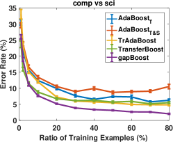
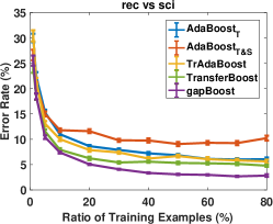
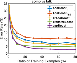
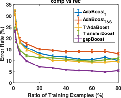
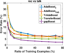
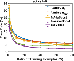
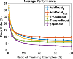
Figure 1: Test error rates (%) with different sizes of target sample on different tasks and on average across all tasks. $\operatorname{\mathsf{gapBoost}}$ consistently outperforms the baselines on all regimes of target sample size. Since $\operatorname{\mathsf{gapBoost}}$ more effectively leverages the target instances, its improvement over the baselines is more noticeable as the target sample size increases. Error bars represent standard error.

6.1.3 Parameter sensitivity

Next, we empirically evaluated our algorithms’ sensitivity to the choice of hyper-parameters. We first fixed $\rho_{\mathcal{T}}=0$ and varied $\exp(\rho_{\mathcal{S}})$ in the range of $[0.1,\dots,0.9]$. Figure 2 shows the results averaged over all transfer problems on the 20 Newsgroups data set, showing that as the size of the target sample increases, the influence of the hyper-parameter on performance decreases. In particular, we see that we are able to obtain a range of hyper-parameters for which our method outperforms all baselines in all sample size regimes.

6.1.4 Increase the weight of a target instance when auxiliary learners coincide

To further minimize the gap, we can modify the weight update rule for target data: $\beta^{\mathcal{T}}=\rho_{\mathcal{T}}\mathbbm{1}_{h_{k}^{\mathcal{S}}(x^{\mathcal{T}})=h_{k}^{\mathcal{T}}(x^{\mathcal{T}})}+\alpha_{k}\mathbbm{1}_{h_{k}(x^{\mathcal{T}})\neq y^{\mathcal{T}}}$ with $\rho_{\mathcal{T}}\geq 0$. We vary $\rho_{\mathcal{S}}$ and $\rho_{\mathcal{T}}$ together, and the results are shown in Figure 3. It can be observed that $\operatorname{\mathsf{gapBoost}}$ can achieve even better performance by focusing more on performance gap minimization (i.e., choosing large $\rho_{\mathcal{S}}$ and $\rho_{\mathcal{T}}$). As the target data increase, the results are less sensitive to the hyper-parameters.

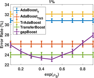
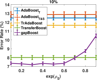
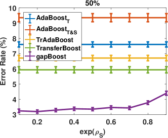
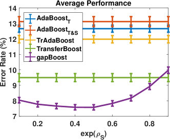
Figure 2: Test error rates (%) averaged across all tasks with respect to the values of the hyper-parameter $\rho_{\mathcal{S}}$ for varying sample sizes. The rightmost graphic shows results averaged over all sample sizes. $\operatorname{\mathsf{gapBoost}}$ becomes less sensitive to the choice of $\rho_{\mathcal{S}}$ as the target sample grows larger. In all cases, there is a range of $\rho_{\mathcal{S}}$ that outperforms all baselines. Error bars represent standard error.

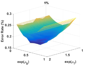
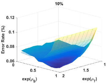
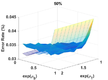
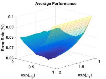
Figure 3: Test error rates ($\%$) with varying $\rho_{\mathcal{S}}$ and $\rho_{\mathcal{T}}$. The valley curves correspond to $\rho_{\mathcal{T}}=0$ (i.e., the purple curves in Figure 2). Hence, regions below the curve indicate better hyper-parameters.

6.2 Multitask Learning

Next, we examined $\operatorname{\mathsf{gapMTNN}}$ on four benchmark data sets: Digits (Shui et al., 2019), PACS (Li et al., 2017), Office-31 (Saenko et al., 2010), and Office-Home (Venkateswara et al., 2017). The Digits data set consists of tasks: MNIST, MNIST_M (M-M), and SVHN, with 10 digit classes in each task. The PACS data set consists of images from four tasks: Photo (P), Art painting (A), Cartoon (C), Sketch (S), with 7 different categories in each task. The Office-31 data set is a vision benchmark consisting of three different tasks: Amazon, Dslr and Webcam, with 31 classes in each task. Office-Home is a more challenging benchmark with four different tasks: Art (Ar.), Clipart (Cl.), Product (Pr.) and Real World (Rw.), each of which has 65 categories.

Table 4: Comparison of different methods on the Digits data set in terms of error rate (%). $\operatorname{\mathsf{gapMTNN}}$ outperforms all baselines in terms of average performance.

		Uniform	Weighted	Adv.H	Adv.W	Multi-Obj	AMTNN	$\operatorname{\mathsf{gapMTNN}}$
$3K$	MNIST	$6.07_{\pm 3.24}$	$10.69_{\pm 3.31}$	$9.90_{\pm 1.21}$	$3.21_{\pm 0.62}$	$\bf 2.48_{\pm 0.27}$	$3.13_{\pm 0.22}$	$3.23_{\pm 0.28}$
	SVHN	$42.73_{\pm 0.42}$	$29.78_{\pm 1.78}$	$29.18_{\pm 0.51}$	$30.50_{\pm 1.06}$	$45.22_{\pm 0.32}$	$22.86_{\pm 0.92}$	$\bf{19.62}_{\pm 0.42}$
	MNIST_M	$22.88_{\pm 2.58}$	$23.62_{\pm 3.05}$	$18.80_{\pm 1.33}$	$\bf 18.67_{\pm 0.71}$	$23.09_{\pm 0.53}$	$19.18_{\pm 1.54}$	$18.98_{\pm 0.51}$
	avg.	$23.89$	$21.36$	$19.29$	$17.46$	$23.60$	$15.07$	$\bf 13.94$
$5K$	MNIST	$3.75_{\pm 1.19}$	$8.20_{\pm 2.71}$	$8.13_{\pm 2.57}$	$2.52_{\pm 0.15}$	$\bf 1.78_{\pm 0.21}$	$2.28_{\pm 0.14}$	$2.54_{\pm 0.40}$
	SVHN	$31.97_{\pm 2.93}$	$26.40_{\pm 3.11}$	$26.40_{\pm 1.61}$	$27.37_{\pm 1.22}$	$38.84_{\pm 0.80}$	$21.60_{\pm 0.78}$	$\bf{17.47}_{\pm 0.47}$
	MNIST_M	$20.86_{\pm 3.12}$	$25.76_{\pm 0.88}$	$\bf 16.27_{\pm 1.37}$	$16.58_{\pm 0.41}$	$19.78_{\pm 0.74}$	$16.43_{\pm 1.13}$	$17.54_{\pm 1.91}$
	avg.	$18.86$	$20.12$	$16.93$	$15.49$	$20.13$	$13.44$	$\bf 12.52$
$8K$	MNIST	$2.26_{\pm 0.50}$	$7.66_{\pm 2.59}$	$5.07_{\pm 1.58}$	$1.89_{\pm 0.32}$	$\bf 1.50_{\pm 0.31}$	$1.90_{\pm 0.16}$	$3.04_{\pm 0.05}$
	SVHN	$28.63_{\pm 0.93}$	$25.88_{\pm 1.55}$	$20.86_{\pm 0.31}$	$24.56_{\pm 1.06}$	$30.06_{\pm 0.88}$	$19.79_{\pm 1.34}$	$\bf 15.90_{\pm 0.28}$
	MNIST_M	$16.32_{\pm 2.19}$	$23.12_{\pm 3.07}$	$\bf 14.84_{\pm 0.34}$	$15.70_{\pm 0.43}$	$17.21_{\pm 0.49}$	$16.92_{\pm 2.12}$	$15.46_{\pm 0.35}$
	avg.	$15.74$	$18.89$	$13.59$	$14.05$	$16.27$	$12.87$	$\bf 11.47$

Table 5: Comparison of different methods on the PACS data set in terms of error rate (%). $\operatorname{\mathsf{gapMTNN}}$ outperforms all baselines in most tasks.

		Uniform	Weighted	Adv.H	Adv.W	Multi-Obj	AMTNN	$\operatorname{\mathsf{gapMTNN}}$
$10\%$	A	$21.24_{\pm 1.14}$	$17.32_{\pm 1.08}$	$23.23_{\pm 1.64}$	$21.22_{\pm 1.09}$	$20.58_{\pm 1.81}$	$\mathbf{17.24_{\pm 0.38}}$	$19.37_{\pm 0.42}$
	C	$18.17_{\pm 1.42}$	$13.78_{\pm 0.57}$	$15.68_{\pm 0.42}$	$16.11_{\pm 1.22}$	$16.62_{\pm 1.31}$	$13.33_{\pm 0.38}$	$\mathbf{12.07_{\pm 0.41}}$
	P	$12.91_{\pm 0.37}$	$10.32_{\pm 1.12}$	$11.73_{\pm 0.62}$	$12.43_{\pm 1.38}$	$12.97_{\pm 0.48}$	$8.74_{\pm 0.91}$	$\mathbf{5.57_{\pm 0.51}}$
	S	$16.62_{\pm 0.62}$	$15.10_{\pm 0.71}$	$16.00_{\pm 0.61}$	$15.98_{\pm 0.88}$	$17.08_{\pm 1.05}$	$18.78_{\pm 0.81}$	$\mathbf{8.11_{\pm 0.52}}$
	avg.	$17.24$	$14.13$	$16.66$	$16.44$	$16.81$	$14.52$	$\bf 11.28$
$15\%$	A	$17.21_{\pm 0.82}$	$\mathbf{14.90_{\pm 0.89}}$	$17.36_{\pm 0.83}$	$16.42_{\pm 1.42}$	$17.25_{\pm 0.52}$	$14.90_{\pm 0.32}$	$16.55_{\pm 0.36}$
	C	$13.33_{\pm 0.87}$	$12.14_{\pm 0.72}$	$12.20_{\pm 0.67}$	$15.21_{\pm 0.52}$	$12.45_{\pm 0.44}$	$11.23_{\pm 0.33}$	$\mathbf{10.18_{\pm 0.56}}$
	P	$10.73_{\pm 0.72}$	$8.82_{\pm 1.04}$	$10.08_{\pm 0.67}$	$15.47_{\pm 0.72}$	$10.91_{\pm 0.64}$	$7.13_{\pm 0.44}$	$\mathbf{5.45_{\pm 0.43}}$
	S	$15.09_{\pm 0.67}$	$12.73_{\pm 0.72}$	$13.91_{\pm 0.43}$	$16.03_{\pm 0.56}$	$13.50_{\pm 0.52}$	$14.22_{\pm 0.51}$	$\mathbf{6.87_{\pm 0.42}}$
	avg.	$14.09$	$12.15$	$13.39$	$15.78$	$13.53$	$11.87$	$\bf 9.76$
$20\%$	A	$15.91_{\pm 0.89}$	$13.88_{\pm 0.56}$	$15.64_{\pm 0.70}$	$16.45_{\pm 0.47}$	$15.73_{\pm 0.88}$	$\mathbf{12.64_{\pm 0.22}}$	$13.67_{\pm 0.30}$
	C	$12.11_{\pm 0.82}$	$10.27_{\pm 0.42}$	$12.36_{\pm 0.33}$	$10.45_{\pm 0.73}$	$11.27_{\pm 0.40}$	$10.09_{\pm 0.56}$	$\mathbf{8.40_{\pm 0.43}}$
	P	$9.52_{\pm 0.61}$	$7.91_{\pm 1.23}$	$8.54_{\pm 0.42}$	$8.62_{\pm 0.45}$	$9.02_{\pm 0.33}$	$6.27_{\pm 0.39}$	$\mathbf{4.47_{\pm 0.44}}$
	S	$14.21_{\pm 1.21}$	$11.64_{\pm 0.89}$	$11.68_{\pm 0.41}$	$12.73_{\pm 0.56}$	$11.2_{\pm 0.73}$	$12.27_{\pm 0.12}$	$\mathbf{6.16_{\pm 0.44}}$
	avg.	$12.94$	$10.93$	$12.06$	$12.06$	$11.81$	$10.32$	$\bf 8.18$

Table 6: Comparison of different methods on the Office-31 data set in term of error rate (%). $\operatorname{\mathsf{gapMTNN}}$ outperforms all baselines in the majority of tasks.

		Uniform	Weighted	Adv.H	Adv.W	Multi-Obj	AMTNN	$\operatorname{\mathsf{gapMTNN}}$
$5\%$	Amazon	$38.73_{\pm 1.32}$	$36.69_{\pm 0.23}$	$34.21_{\pm 1.12}$	$33.50_{\pm 1.89}$	$\mathbf{31.13_{\pm 1.18}}$	$36.67_{\pm 0.60}$	$31.77_{\pm 1.67}$
	Dslr	$28.18_{\pm 2.12}$	$\bf 12.57_{\pm 2.33}$	$26.45_{\pm 0.78}$	$28.18_{\pm 1.09}$	$27.51_{\pm 1.44}$	$19.88_{\pm 1.56}$	${13.25}_{\pm 1.40}$
	Webcam	$27.88_{\pm 1.12}$	$15.09_{\pm 0.56}$	$28.64_{\pm 0.72}$	$30.08_{\pm 0.92}$	$27.73_{\pm 0.41}$	$14.64_{\pm 0.30}$	$\mathbf{14.18_{\pm 0.89}}$
	avg.	$31.60$	$21.45$	$29.77$	$30.59$	$28.79$	$23.73$	$\bf 19.73$
$10\%$	Amazon	$26.82_{\pm 0.51}$	$29.36_{\pm 1.21}$	$28.98_{\pm 0.89}$	$25.31_{\pm 1.13}$	$25.36_{\pm 0.89}$	$28.73_{\pm 1.20}$	$\mathbf{23.56_{\pm 0.63}}$
	Dslr	$19.36_{\pm 1.44}$	$7.91_{\pm 0.91}$	$15.91_{\pm 0.91}$	$14.09_{\pm 0.80}$	$13.18_{\pm 1.12}$	$\mathbf{7.21_{\pm 0.89}}$	${7.87}_{\pm 1.81}$
	Webcam	$17.89_{\pm 0.91}$	$11.60_{\pm 1.33}$	$10.56_{\pm 0.14}$	$14.31_{\pm 0.78}$	$13.08_{\pm 0.78}$	$10.41_{\pm 1.21}$	$\mathbf{8.16_{\pm 1.54}}$
	avg.	$21.36$	$16.29$	$18.48$	$17.90$	$17.21$	$15.45$	$\bf 13.20$
$20\%$	Amazon	$20.56_{\pm 0.84}$	$23.21_{\pm 0.93}$	$20.31_{\pm 0.53}$	$20.73_{\pm 0.56}$	$20.77_{\pm 0.78}$	$19.80_{\pm 0.91}$	$\mathbf{17.38_{\pm 0.89}}$
	Dslr	$8.82_{\pm 1.01}$	$\mathbf{3.40}_{\pm 0.71}$	$6.31_{\pm 0.67}$	$6.17_{\pm 0.44}$	$7.91_{\pm 0.63}$	$5.82_{\pm 1.22}$	$3.65_{\pm 0.81}$
	Webcam	$6.91_{\pm 0.82}$	$4.40_{\pm 0.52}$	$6.32_{\pm 0.64}$	$7.77_{\pm 0.90}$	$5.26_{\pm 0.56}$	$5.58_{\pm 0.89}$	$\bf{4.08_{\pm 0.72}}$
	avg.	$12.10$	$10.34$	$10.98$	$11.56$	$11.31$	$10.40$	$\bf 8.37$

Table 7: Comparison of different methods on the Office-Home data set in terms of error rate (%). $\operatorname{\mathsf{gapMTNN}}$ outperforms all baselines in most tasks.

		Uniform	Weighted	Adv.H	Adv.W	Multi-Obj	AMTNN	$\operatorname{\mathsf{gapMTNN}}$
5%	Ar.	$73.82_{\pm 0.31}$	$73.18_{\pm 1.56}$	$72.27_{\pm 1.44}$	$73.21_{\pm 0.82}$	$74.36_{\pm 1.50}$	$67.50_{\pm 1.33}$	$\bf 61.91_{\pm 0.35}$
	Cl.	$69.91_{\pm 0.22}$	$68.78_{\pm 1.83}$	$67.94_{\pm 1.45}$	$67.31_{\pm 0.45}$	$68.29_{\pm 1.71}$	$65.45_{\pm 0.90}$	$\bf 60.01_{\pm 1.02}$
	Pr.	$42.36_{\pm 0.13}$	$40.81_{\pm 0.43}$	$40.44_{\pm 0.73}$	$41.70_{\pm 0.89}$	$41.32_{\pm 1.32}$	$43.72_{\pm 0.78}$	$\bf 37.85_{\pm 0.82}$
	Rw.	$52.60_{\pm 1.11}$	$49.45_{\pm 1.22}$	$48.91_{\pm 0.93}$	$52.92_{\pm 0.37}$	$48.47_{\pm 0.89}$	$50.14_{\pm 1.75}$	$\bf 43.96_{\pm 0.27}$
	avg.	$59.67$	$58.06$	$57.39$	$58.79$	$58.11$	$56.70$	$\bf 50.93$
10%	Ar.	$64.18_{\pm 0.67}$	$61.81_{\pm 1.03}$	$61.03_{\pm 0.89}$	$61.50_{\pm 0.82}$	$65.38_{\pm 0.92}$	$58.89_{\pm 1.02}$	$\bf 55.67_{\pm 0.70}$
	Cl.	$56.73_{\pm 0.63}$	$54.68_{\pm 1.61}$	$54.21_{\pm 1.78}$	$55.64_{\pm 0.67}$	$56.66_{\pm 1.43}$	$52.45_{\pm 0.83}$	$\bf 48.50_{\pm 0.87}$
	Pr.	$32.86_{\pm 0.42}$	$30.88_{\pm 0.23}$	$30.61_{\pm 0.41}$	$32.44_{\pm 0.67}$	$33.85_{\pm 1.50}$	$31.61_{\pm 0.72}$	$\bf 28.76_{\pm 0.45}$
	Rw.	$43.18_{\pm 1.31}$	$41.67_{\pm 0.78}$	$41.20_{\pm 0.56}$	$40.46_{\pm 0.89}$	$43.19_{\pm 0.73}$	$41.10_{\pm 0.90}$	$\bf 37.82_{\pm 0.27}$
	avg.	$49.24$	$47.26$	$46.76$	$47.51$	$49.77$	$46.01$	$\bf 42.69$
20%	Ar.	$54.54_{\pm 0.82}$	$52.07_{\pm 0.12}$	$53.34_{\pm 0.51}$	$52.12_{\pm 0.49}$	$53.80_{\pm 0.82}$	$\bf 51.11_{\pm 0.50}$	$51.20_{\pm 1.03}$
	Cl.	$43.88_{\pm 0.61}$	$43.29_{\pm 0.89}$	$43.45_{\pm 1.13}$	$43.33_{\pm 0.56}$	$43.44_{\pm 0.50}$	${39.34}_{\pm 0.41}$	$\bf 39.15_{\pm 0.93}$
	Pr.	$25.62_{\pm 0.67}$	$24.36_{\pm 0.56}$	$24.38_{\pm 0.43}$	$24.59_{\pm 1.12}$	$25.74_{\pm 0.67}$	$24.64_{\pm 0.40}$	$\bf 23.45_{\pm 0.78}$
	Rw.	$37.41_{\pm 0.62}$	$35.20_{\pm 0.89}$	$34.88_{\pm 0.74}$	$34.30_{\pm 0.78}$	$37.24_{\pm 0.56}$	$35.31_{\pm 0.44}$	$\bf 33.38_{\pm 0.73}$
	avg.	$40.36$	$38.73$	$39.01$	$38.59$	$40.06$	$37.60$	$\bf 36.80$

Following the evaluation protocol in prior work (Long et al., 2015; Shui et al., 2019; Zhou et al., 2021a), we evaluated $\operatorname{\mathsf{gapMTNN}}$ against the baselines when only part of the data is available. For the Digits data set, we randomly select $3K$, $5K$ and $8K$ instances for training. For the SVHN data set, we resize the images to $28\times 28\times 1$; we do not apply any data augmentation on the Digits data set. A LeNet-5 (LeCun et al., 1998) model is implemented as the feature extractor and three 3-layer MLPs are deployed as task-specific classifiers, with the features from the classifier being of size $128$. For the experiments on PACS data set, we randomly selected $10\%$, $15\%$ and $20\%$ of the total training data for training. We adopted the pre-trained AlexNet model (PyTorch implementation; (Paszke et al., 2019)) as a feature extractor, removing the last fully-connected layers, yielding a feature dimension of size 4096. For the Office-31 and Office-Home data sets, we adopted the ResNet-18 model as a feature extractor by also removing the last fully-connected layers of the original implementations, yielding a feature dimension of size 512. We followed the evaluation protocol of (Zhou et al., 2021a) by choosing $5\%$, $10\%$ and $20\%$ of the data for training. We trained the networks using the Adam optimizer, with an initial learning rate of $2e-4$, decaying by $5\%$ every $5$ epochs, for a total of $120$ epochs. Additional details on the experimental implementation can be found in Appendix C.

6.2.1 Performance Comparison

We adopted the following algorithms as baselines:

• Uniform: Treating all the tasks equally without any task alignments for training the deep networks.

• Weighted: Adapted from (Murugesan et al., 2016), apply a weighted risk over all the tasks, where the weights are determined based on a probabilistic interpretation.

• Adv.H: Implementing the method of (Liu et al., 2017a) with the same loss function while training with $\mathcal{H}$-divergence as the adversarial objective.

• Adv.W: Implementing the method of (Liu et al., 2017a) with the same loss function while training with the Wasserstein distance based adversarial training method.

• Multi-Obj: Treating the multitask learning problem as a multi-objective problem (Sener and Koltun, 2018).

• AMTNN: A Wasserstein adversarial training method for estimating the task relations (Shui et al., 2019).

The results on Digits, PACS, Office-31, and Office-Home data sets are, respectively, reported in Tables 4 – 7. It can be observed that $\operatorname{\mathsf{gapMTNN}}$ outperforms the baselines in most cases. In particular, compared with AMTNN, which only aligns marginal distributions, $\operatorname{\mathsf{gapMTNN}}$ has a large margin of improvement especially when there are few labeled instances (e.g., 5% of the total instances), which confirms the effectiveness of our methods when dealing with limited data.

6.2.2 Visualizations of Task Relation Coefficients

In order to further verify the task weighting principles of $\operatorname{\mathsf{gapMTNN}}$, we visualize the task relation coefficients $\Gamma$ learned from the Digits data set, as shown in Figure 4. From the figure, we observe the following: (1) the task coefficients are non-uniform and asymmetric, which highlights the importance of properly choosing the coefficients for combining the tasks rather than simply treating them equally. (2) The coefficients between MNIST and MNIST_M are higher than the coefficients between SVHN and MNIST or MNIST_M, which is reasonable as SVHN is less related to the other tasks (Shui et al., 2019). (3) MNIST is assigned a higher weight to itself than the other tasks (see the diagonal entries of the matrices). This can be due to the fact that MNIST is a relatively easy task, and therefore can be learned well without leveraging the knowledge from other tasks too much. (4) From left to right, the values of diagonal entries of the matrices indicate that each task relies on the other tasks less as the number of training instances increases. This is also reasonable since once the sample size of each individual task becomes larger, the benefit of knowledge transfer and sharing is less significant for multitask learning.

Figure 4: Task relation coefficient matrices learned by $\operatorname{\mathsf{gapMTNN}}$ on the Digits data set with training set of $3K$, $5K$, and $8K$ instances, respectively

6.2.3 Running Time Comparison

To show the efficiency of the $\operatorname{\mathsf{gapMTNN}}$ method, we compared its training time against the baselines. Specifically, we evaluated multitask learning algorithms on the Digits ($8K$), PACS ($20\%$), Office-31 ($20\%$) and Office-Home ($20\%$) data sets, and report the relative time comparison of one training epoch in a relative percentage bar chart in Fig. 5. It can be observed that as $\operatorname{\mathsf{gapMTNN}}$ adopts the centroid alignment strategy, it achieves comparable efficiency with Multi-Obj, and is more efficient than the adversarial training based methods (e.g., Adv.H, Adv.W and AMTNN), especially on the Office-Home data set. Taking the results reported in Tables 4 – 7 into consideration, $\operatorname{\mathsf{gapMTNN}}$ can improve the performances on the benchmark data sets while reducing the time needed for training.

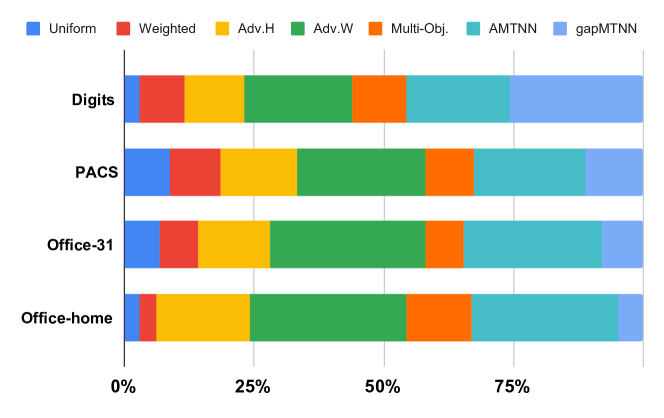
Figure 5: Time comparison on different data sets.

6.2.4 Ablation Studies

We conducted ablation studies on the Office-31 data set with 20% of the data to verify each component of $\operatorname{\mathsf{gapMTNN}}$. We compared the full version of $\operatorname{\mathsf{gapMTNN}}$ with the following ablated versions: (1) cls. only: train the model uniformly with only the classification objective. (2) w/o marginal alignment: we omit the marginal alignment objective and train the model with semantic matching and task relation optimization. (3) w/o semantic matching: we omit the semantic conditional distribution matching objective and train the model with marginal alignment objective with task relation optimization. (4) w/o cvx opt.: we omit task relation estimations and train the model with marginal alignment and semantic matching objectives. (5) w/o marginal $\&$ semantic: we remove both adversarial and semantic learning objectives. The results of the ablation studies are presented in Table 8, showing that distribution matching is crucial for the algorithm. Both marginal and conditional distribution matching improve learning performance.

Table 8: Ablation studies on Office-31 data set.

Method	Amazon	Dslr	WebCam	Avg.
Cls. only	$20.6_{\pm 0.8}$	$8.8_{\pm 1.0}$	$6.9_{\pm 0.8}$	$12.1$
w/o marginal	$18.9_{\pm 0.2}$	$3.5_{\pm 0.1}$	$3.9_{\pm 0.2}$	$8.8$
w/o sem. matching	$18.8_{\pm 1.1}$	$3.4_{\pm 0.7}$	$4.8_{\pm 0.4}$	$9.0$
w/o cvx opt.	$18.2_{\pm 0.3}$	$4.7_{\pm 0.9}$	$3.8_{\pm 0.5}$	$8.9$
w/o marginal $\&$ sem. matching	$20.2_{\pm 0.5}$	$3.9_{\pm 0.3}$	$4.6_{\pm 0.3}$	$9.6$
Full method	$17.4_{\pm 0.9}$	$3.7_{\pm 0.8}$	$4.1\pm 0.7$	$8.4$

7 Conclusion

In this paper, we propose the notion of performance gap to measure the discrepancy between the tasks with labeled instances. We relate this notion with the model complexity and show that it can be viewed as a data- and algorithm-dependent regularizer, which eventually leads to gap minimization, a general principle that is applicable to both transfer learning and multitask learning. We propose $\operatorname{\mathsf{gapBoost}}$, $\operatorname{\mathsf{gapBoostR}}$, and $\operatorname{\mathsf{gapMTNN}}$ as three algorithmic instantiations that exploit the gap minimization principle. The empirical evaluation justifies the effectiveness of our algorithms.

The principle of performance gap minimization opens up several avenues for knowledge sharing and transfer. For example, it could be used to analyze strategies for other knowledge sharing and transfer scenarios such as domain generalization, multi-label learning, lifelong learning, or even knowledge transfer across different learning paradigms (e.g., between classification and regression). It could also be adopted for fair learning (Shui et al., 2022a, d). On the theoretical side, future directions could include extending the notion of performance gap to unlabeled data for domain adaptation, and to non-stationary environments. We plan to explore these questions in future work.

Appendix A Proof of Theoretical Results

A.1 Instance Weighting

In order to prove Theorem 6, we need some auxiliary results.

Lemma 42

Let $\mathcal{L}^{\Gamma}_{\mathcal{D}}=\mathcal{L}_{\mathcal{D}_{1}}^{\Gamma^{1}}+\mathcal{L}_{\mathcal{D}_{2}}^{\Gamma^{2}}$. Then, for any $h\in\mathcal{H}$, we have

$$\mathcal{L}_{\mathcal{D}_{1}}(h)\leq\mathcal{L}_{\mathcal{D}}^{\Gamma}+\|\Gamma^{2}\|_{1}\operatorname{dist}_{\mathcal{Y}}(\mathcal{D}_{1},\mathcal{D}_{2})\enspace.$$

Proof 

$$\mathcal{L}_{\mathcal{D}_{1}}(h)-\mathcal{L}_{\mathcal{D}}^{\Gamma}(h) \leq\left|\mathcal{L}_{\mathcal{D}_{1}}(h)-\mathcal{L}_{\mathcal{D}_{1}}^{\Gamma^{1}}(h)-\mathcal{L}_{\mathcal{D}_{2}}^{\Gamma^{2}}(h)\right|$$

$$=\left|\mathcal{L}_{\mathcal{D}_{1}}(h)-(1-\gamma_{2})\mathcal{L}_{\mathcal{D}_{1}}(h)-\gamma_{2}\mathcal{L}_{\mathcal{D}_{2}}(h)\right|$$ linearity of expectation

$$=\|\Gamma^{2}\|_{1}\left|\mathcal{L}_{\mathcal{D}_{1}}(h)-\mathcal{L}_{\mathcal{D}_{2}}(h)\right|$$

$$\leq\|\Gamma^{2}\|_{1}\operatorname{dist}_{\mathcal{Y}}(\mathcal{D}_{1},\mathcal{D}_{2}) \mathcal{Y}$$ definition of -discrepancy distance

 

Definition 43 (Weight dependent uniform stability)

Let $h_{{S}}\in\mathcal{H}$ be the hypothesis returned by a learning algorithm $\mathcal{A}$ when trained on sample $S$ weighted by $\Gamma$. An algorithm $\mathcal{A}$ has weight dependent uniform stability, with $\beta_{i}\geq 0$, if the following holds:

$$\sup_{z\sim\mathcal{D}}\left|\ell(h_{S}(x),y)-\ell(h_{S^{i}}(x),y)\right|\leq\beta_{i}\enspace,\qquad\forall{S},{S}^{i}$$

where ${S}^{i}$ is the training sample ${S}$ with the $i$-th example $z_{i}$ replaced by an i.i.d. example $z_{i}^{\prime}$.

We bound the generalization error for weight dependent stable algorithms.

Lemma 44

Assume that the loss function is upper bounded by $B\geq 0$. Let $S$ be a training sample of $N$ i.i.d. points drawn from some distribution $\mathcal{D}$, weighted by $\Gamma$, and let $h_{S}$ be the hypothesis returned by a weight dependent stable learning algorithm $\mathcal{A}$. Then, for any $\delta\in(0,1)$, with probability at least $1-\delta$, the following holds:

$$\mathcal{L}_{\mathcal{D}}^{\Gamma}(h_{S})\leq\mathcal{L}_{S}^{\Gamma}(h_{S})+\beta+(\Delta+\beta+\|\Gamma\|_{\infty}B)\sqrt{\frac{N\log\frac{1}{\delta}}{2}}\enspace,$$

where $\beta=\max\{\beta_{i}\}_{i=1}^{N}$, $\Delta=\sum_{i=1}^{N}\gamma_{i}\beta_{i}$ and $\|\Gamma\|_{\infty}=\max\{\gamma_{i}\}_{i=1}^{N}$.

Proof  Let $\Phi^{\Gamma}(S)=\mathcal{L}_{\mathcal{D}}^{\Gamma}(h_{S})-\mathcal{L}_{S}^{\Gamma}(h_{S})$. Then, by the definition of $\Phi^{\Gamma}$, we have

$$|\Phi(S)-\Phi(S^{i})|\leq|\mathcal{L}_{\mathcal{D}}^{\Gamma}(h_{S})-\mathcal{L}_{\mathcal{D}}^{\Gamma}(h_{S^{i}})|+|\mathcal{L}_{S}^{\Gamma}(h_{S})+\mathcal{L}_{S^{i}}^{\Gamma}(h_{S^{i}})|\enspace.$$

By the stability of the algorithm, we have

$$|\mathcal{L}_{\mathcal{D}}^{\Gamma}(h_{S})-\mathcal{L}_{\mathcal{D}}^{\Gamma}(h_{S^{i}})|=|\mathbb{E}_{z\sim\mathcal{D}}[\ell_{z}(h_{S})]-\mathbb{E}_{z\sim\mathcal{D}}[\ell_{z}(h_{S^{i}})]|\leq\beta\enspace,$$

where $\beta=\max\{\beta_{i}\}_{i=1}^{N}$. In addition, we also have

$$|\mathcal{L}_{S}^{\Gamma}(h_{S})-\mathcal{L}_{S^{i}}^{\Gamma}(h_{S^{i}})| =\left|\sum_{j\neq i}\gamma_{j}(\ell_{z_{j}}(h_{S})-\ell_{z_{j}}(h_{S^{i}}))+\gamma_{i}(\ell_{z_{i}}(h_{S})-\ell_{z_{i}^{\prime}}(h_{S^{i}}))\right|$$

$$\leq\left|\sum_{j\neq i}\gamma_{j}\left|\ell_{z_{j}}(h_{S})-\ell_{z_{j}}(h_{S^{i}})\right|+\gamma_{i}\left|\ell_{z_{i}}(h_{S})-\ell_{z_{i}^{\prime}}(h_{S^{i}})\right|\right|$$

$$\leq\sum_{j\neq i}\gamma_{j}\beta_{j}+\gamma_{i}B$$

$$\leq\Delta+\|\Gamma\|_{\infty}B$$

Consequently, $\Phi^{\Gamma}$ satisfies $|\Phi^{\Gamma}(S)-\Phi^{\Gamma}(S^{i})|\leq\sum_{i=1}^{N}\gamma_{i}\beta_{i}+\beta+\|\Gamma\|_{\infty}B$. By applying McDiarmid’s inequality, we have

$$\text{Pr}\left[\Phi(S)\geq\epsilon+\mathbb{E}[\Phi(S)]\right]\leq\exp\left(\frac{-2\epsilon^{2}}{N\left(\Delta+\beta+\|\Gamma\|_{\infty}B\right)^{2}}\right)\enspace.$$ (14)

By setting $\delta=\exp\left(\frac{-2\epsilon^{2}}{N\left(\Delta+\beta+\|\Gamma\|_{\infty}B\right)^{2}}\right)$, we obtain $\epsilon=\left(\Delta+\beta+\|\Gamma\|_{\infty}B\right)\sqrt{\frac{N\log\frac{1}{\delta}}{2}}$. Plugging $\epsilon$ back to (14) and rearranging terms, with probability $1-\delta$, we have

$$\Phi(S)\leq\mathbb{E}[\Phi(S)]+\left(\Delta+\beta+\|\Gamma\|_{\infty}B\right)\sqrt{\frac{N\log\frac{1}{\delta}}{2}}\enspace.$$ (15)

By the linearity of expectation, we have $\mathbb{E}[\Phi(S)]=\mathbb{E}_{S\sim\mathcal{D}^{N}}[\mathcal{L}^{\Gamma}_{\mathcal{D}}(h_{S})]-\mathbb{E}_{S\sim\mathcal{D}^{N}}[\mathcal{L}_{S}^{\Gamma}(h_{S})]$. By the definition of the generalization error, we have

$$\mathbb{E}_{S\sim\mathcal{D}^{N}}[\mathcal{L}^{\Gamma}_{\mathcal{D}}(h_{S})]=\mathbb{E}_{S,z\sim\mathcal{D}^{N+1}}[\ell_{z}(h_{S})]\enspace.$$

On the other hand, by the linearity of expectation, we have

$$\mathbb{E}_{S\sim\mathcal{D}^{N}}[\mathcal{L}_{S}^{\Gamma}(h_{S})]=\mathbb{E}_{S\sim\mathcal{D}^{N}}\left[\sum_{i=1}^{N}\gamma_{i}\ell_{z_{i}}(h_{S})\right]=\mathbb{E}_{S,z\sim\mathcal{D}^{N+1}}\left[\ell_{z}(h_{S^{\prime}})\right]\enspace,$$

where $S^{\prime}$ is a sample of $N$ data points containing $z$ drawn from the data set $\{S,z\}$. Therefore, we have

$$\mathbb{E}[\Phi(S)] \leq\left|\mathbb{E}_{S,z\sim\mathcal{D}^{N+1}}[\ell_{z}(h_{S})]-\mathbb{E}_{S,z\sim\mathcal{D}^{N+1}}\left[\ell_{z}(h_{S^{\prime}})\right]\right|$$

$$\leq\mathbb{E}_{S,z\sim\mathcal{D}^{N+1}}\left[\left|\ell_{z}(h_{S})-\ell_{z}(h_{S^{\prime}})\right|\right]$$ Jensen’s inequality

$$\leq\beta$$

Replacing $\mathbb{E}[\Phi(S)]$ by $\beta$ in Eq. (15) completes the proof.  

Lemma 45 shows that the instance weighting algorithm has weight dependent stability.

Lemma 45

The instance weighting transfer learning algorithm with a $\rho$-Lipschitz continuous loss function and the regularizer $\mathcal{R}(h)=\|h\|_{2}^{2}$ has weight dependent uniform stability, with

$$\beta_{i}\leq\frac{\gamma_{i}\rho^{2}R^{2}}{\lambda}\enspace.$$

Proof  Let $\mathcal{V}_{S}(h)=\mathcal{L}^{\Gamma}_{S}(h)+\lambda\mathcal{R}(h)$. By the definition of Bregman divergence, we have

$$d_{\mathcal{V}_{{S}^{i}}}\big{(}{h}_{{S}},{h}_{{S}^{i}}\big{)}+d_{\mathcal{V}_{{S}}}\big{(}{h}_{{S}^{i}},{h}_{{S}}\big{)} =\mathcal{L}^{\Gamma}_{{S}^{i}}\big{(}{h}_{{S}}\big{)}-\mathcal{L}^{\Gamma}_{{S}^{i}}\big{(}{h}_{{S}^{i}}\big{)}+\mathcal{L}^{\Gamma}_{{S}}\big{(}{h}_{{S}^{i}}\big{)}-\mathcal{L}^{\Gamma}_{{S}}\big{(}{h}_{{S}}\big{)}$$

$$=\gamma_{i}\left(\ell(\langle{h}_{{S}},x_{i}^{\prime}\rangle,y_{i}^{\prime})-\ell(\langle{h}_{{S}^{i}},x_{i}^{\prime}\rangle,y_{i}^{\prime})+\ell(\langle{h}_{{S}^{i}},x_{i}\rangle,y_{i})-\ell(\langle{h}_{{S}},{x_{i}}\rangle,{y_{i}})\right)$$

$$\leq\gamma_{i}\left(\rho\left|\langle{h}_{{S}}-{h}_{{S}^{i}},x_{i}^{\prime}\rangle\right|+\rho\left|\langle{h}_{{S}}-{h}_{{S}^{i}},x_{i}\rangle\right|\right)$$

$$\leq 2\gamma_{i}\rho R\left|\left|{h}_{{S}}-{h}_{{S}^{i}}\right|\right|_{2}$$

where $h_{{S}}$ and $h_{{S}^{i}}$ are, respectively, the optimal solutions of $\mathcal{V}_{S}$ and $\mathcal{V}_{{S}^{i}}$. The first equality holds because of the first-order optimality condition (Boyd and Vandenberghe, 2004) of $\mathcal{V}_{S}$ and $\mathcal{V}_{{S}^{i}}$, and the last two inequalities are, respectively, due to the Lipschitz continuity of loss function $\ell$ and the Cauchy-Schwarz inequality.

Since $d_{\lambda\mathcal{R}}({h}_{{S}},{h}_{{S}^{i}})=d_{\lambda\mathcal{R}}({h}_{{S}^{i}},{h}_{{S}})=\lambda\|{h}_{{S}}-{h}_{{S}^{i}}\|_{2}^{2}$, by the non-negative and additive properties of Bregman divergence, we have

$$\lambda\|{h}_{{S}}-{h}_{{S}^{i}}\|_{2}^{2}\leq\gamma_{i}\rho R\left|\left|{h}_{{S}}-{h}_{{S}^{i}}\right|\right|_{2}\enspace,$$

which gives

$$\|{h}_{{S}}-{h}_{{S}^{i}}\|_{2}\leq\frac{\gamma_{i}\rho R}{\lambda}\enspace.$$

Consequently, by the Lipschitz continuity of $\ell$ and the Cauchy-Schwarz inequality, we have

$$\beta_{i}\leq\frac{\gamma_{i}\rho^{2}R^{2}}{\lambda}\enspace.$$

 

Proof [Proof of Theorem 6] Combining Lemmas 42, 44 and Lemma 45, we immediately obtain Theorem 6  

Proof [Proof of Lemma 8] By the definition of $h_{\mathcal{T}}$, $h_{\mathcal{S}}$, and $h^{*}$, we have

$$\mathcal{V}_{\mathcal{S}}(h_{\mathcal{S}})\leq\mathcal{V}_{\mathcal{S}}(h^{*}),\quad\text{and}\quad\mathcal{V}_{\mathcal{T}}(h_{\mathcal{T}})\leq\mathcal{V}_{\mathcal{T}}(h^{*})\enspace,$$

which gives

$$\mathcal{V}_{\mathcal{S}}(h_{\mathcal{S}})+\mathcal{V}_{\mathcal{T}}(h_{\mathcal{T}})\leq\mathcal{V}(h^{*})+(2\eta-1)\lambda\mathcal{R}(h^{*})\enspace.$$ (16)

On the other hand, we also have

$$\mathcal{V}(h^{*})\leq\mathcal{V}(h_{\mathcal{S}})\enspace,$$ (17)

and

$$\mathcal{V}(h^{*})\leq\mathcal{V}(h_{\mathcal{T}})\enspace.$$ (18)

From (16) and (17), we have

$$\lambda(1-2\eta)\mathcal{R}(h^{*}) \leq\mathcal{V}(h^{*})-\mathcal{V}_{\mathcal{S}}(h_{\mathcal{S}})-\mathcal{V}_{\mathcal{T}}(h_{\mathcal{T}})$$ (19)

$$\leq\mathcal{V}(h_{\mathcal{S}})-\mathcal{V}_{\mathcal{S}}(h_{\mathcal{S}})-\mathcal{V}_{\mathcal{T}}(h_{\mathcal{T}})$$

$$=\nabla_{\mathcal{T}}+\lambda(1-\eta)\mathcal{R}(h_{\mathcal{S}})-\eta\lambda\mathcal{R}(h_{\mathcal{T}})$$

Similarly, from (16) and (18), we also have

$$\lambda(1-2\eta)\mathcal{R}(h^{*})\leq\nabla_{\mathcal{S}}+\lambda(1-\eta)\mathcal{R}(h_{\mathcal{T}})-\eta\lambda\mathcal{R}(h_{\mathcal{S}})$$ (20)

Combining (19) and (20) gives

$$\mathcal{R}(h^{*})\leq\frac{\nabla}{2\lambda(1-2\eta)}+\frac{1}{2}\left(\mathcal{R}(h_{\mathcal{S}})+\mathcal{R}(h_{\mathcal{T}})\right)\enspace.$$

Substituting $\mathcal{R}(h)=\|h\|_{2}^{2}$ concludes the proof.  

A.2 Feature Representation

Proof [Proof of Theorem 12] Following a similar proof for Theorem 6, we can first show that

$$\mathcal{L}_{\mathcal{D}_{\mathcal{T}}}(h\circ\Phi)-\mathcal{L}_{\mathcal{D}}(h\circ\Phi)\leq\frac{N_{\mathcal{S}}}{N}|\mathcal{L}_{\mathcal{D}_{\mathcal{T}}}(h\circ\Phi)-\mathcal{L}_{\mathcal{D}_{\mathcal{S}}}(h\circ\Phi)|\leq\frac{N_{\mathcal{S}}}{N}\text{dist}_{\mathcal{Y}}(\mathcal{D}_{{\mathcal{T}}}^{\Phi},\mathcal{D}_{{\mathcal{S}}}^{\Phi})\enspace.$$ (21)

Similarly, we also have

$$\mathcal{L}_{\mathcal{D}}(h_{S}\circ\Phi)\leq\mathcal{L}_{S}(h_{S}\circ\Phi)+\beta+(2N\beta+B)\sqrt{\frac{\log(\frac{1}{\delta})}{2N}}\enspace,$$ (22)

and

$$\beta\leq\frac{\rho^{2}R^{2}}{\lambda N}\enspace.$$ (23)

Combining (21), (22) and (23), we immediately obtain Theorem 12.  

A.3 Hypothesis Transfer

Proof [Proof of Theorem 17] The proof of Theorem 17 follows readily from Theorem 14.2 and Proposition 14.4 in (Mohri et al., 2018), and therefore is omitted here.  

Proof [Proof of Lemma 19] Let $\mathcal{V}(h)=\mathcal{L}_{S_{\mathcal{T}}}(h)+\lambda||h-\langle H,\Xi\rangle||_{2}^{2}$. By the definition of $h^{*}$, we have

$$\mathcal{V}(h^{*})\leq\mathcal{V}({\langle H,\Xi\rangle}) \Rightarrow\mathcal{L}_{S_{\mathcal{T}}}(h^{*})+\lambda||h^{*}-\langle H,\Xi\rangle||_{2}^{2}\leq\mathcal{L}_{S_{\mathcal{T}}}(\langle H,\Xi\rangle)$$

$$\Rightarrow||h^{*}-\langle H,\Xi\rangle||_{2}\leq\sqrt{\frac{\mathcal{L}_{S_{\mathcal{T}}}(\langle H,\Xi\rangle)-\mathcal{L}_{S_{\mathcal{T}}}(h^{*})}{\lambda}}$$

$$\Rightarrow||h^{*}||_{2}\leq\sqrt{\frac{\mathcal{L}_{S_{\mathcal{T}}}(\langle H,\Xi\rangle)-\mathcal{L}_{S_{\mathcal{T}}}(h^{*})}{\lambda}}+||\langle H,\Xi\rangle||_{2}$$

$$\Rightarrow||h^{*}||_{2}\leq\sqrt{\frac{\mathcal{L}_{S_{\mathcal{T}}}(\langle H,\Xi\rangle)-\mathcal{L}_{S_{\mathcal{T}}}(h_{\mathcal{T}})}{\lambda}}+||\langle H,\Xi\rangle||_{2}$$

 

A.4 Task Weighting

Proof [Proof of Theorem 22] The proof of Theorem 22 follows a similar line as in Theorem 6.

Let $\mathcal{L}_{\mathcal{D}}^{\Gamma^{j}}(h)=\sum_{k=1}^{K}\gamma_{k}^{j}\mathcal{L}_{\mathcal{D}_{k}}(h)$. Then, we have

$$\mathcal{L}_{\mathcal{D}_{j}}(h)-\mathcal{L}_{\mathcal{D}}^{\Gamma^{j}}(h) =\sum_{k=1}^{K}\gamma_{k}^{j}\mathcal{L}_{\mathcal{D}_{j}}(h)-\sum_{k=1}^{K}\gamma_{k}^{j}\mathcal{L}_{\mathcal{D}_{k}}(h)$$ (24)

$$\leq\sum_{k\neq j}\gamma_{k}^{j}\left|\mathcal{L}_{\mathcal{D}_{j}}(h)-\mathcal{L}_{\mathcal{D}_{k}}(h)\right|$$

$$\leq\sum_{k\neq j}\gamma_{k}^{j}\operatorname{dist}_{\mathcal{Y}}(\mathcal{D}_{j},\mathcal{D}_{k})$$

On the other hand, let $h_{S}$ be the hypothesis returned by the task weighting multitask learning approach. Then, by Lemma 44, we also have

$$\mathcal{L}_{\mathcal{D}}^{\Gamma^{j}}(h_{S})\leq\mathcal{L}_{S}^{\Gamma^{j}}(h_{S})+{\beta}^{j}+({\Delta}+{\beta}^{j}+\frac{\|{\Gamma}^{j}\|_{\infty}}{N}B)\sqrt{\frac{KN\log\frac{1}{\delta}}{2}}\enspace,$$ (25)

where ${\beta^{j}}=\max\{{\beta}_{k}^{j}\}_{k=1}^{K}$, and ${\Delta}=\sum_{k=1}^{K}\gamma^{j}_{k}\beta_{k}^{j}$.

Similarly, by Lemma 45, we can prove that

$$\beta_{k}^{j}\leq\frac{\gamma_{k}^{j}\rho^{2}R^{2}}{\lambda N}\enspace.$$ (26)

Combining (24), (25), and (26), we immediately obtain Theorem 22.  

Proof [Proof of Lemma 24] Let $\mathcal{V}(h)=\sum_{k=1}^{K}\gamma_{k}^{j}\mathcal{L}_{k}(h)+\lambda\mathcal{R}(h)$, $\mathcal{V}_{k}(h)=\mathcal{L}_{k}(h)+\eta\lambda\mathcal{R}(h),\forall k=1,\dots,K$. Then, we have

$$\mathcal{V}_{k}(\bar{h}_{k})\leq\mathcal{V}_{k}(h_{j}^{*}) \Rightarrow\sum_{k=1}^{K}\gamma_{k}^{j}\mathcal{V}_{k}(\bar{h}_{k})\leq\sum_{k=1}^{K}\gamma_{k}^{j}\mathcal{V}_{k}(h_{j}^{*})$$

$$\Rightarrow\sum_{k=1}^{K}\gamma_{k}^{j}[\mathcal{L}_{k}(\bar{h}_{k})+\eta\lambda||\bar{h}_{k}||_{2}^{2}]\leq\sum_{k=1}^{K}\gamma_{k}^{j}\mathcal{L}_{k}(h_{j}^{*})+\eta\lambda||h_{j}^{*}||_{2}^{2}$$

On the other hand, for any $\bar{h}_{j}$, we also have

$$\mathcal{V}(h_{j}^{*})\leq\mathcal{V}(\bar{h}_{j})\Rightarrow\sum_{k=1}^{K}\gamma_{k}^{j}\mathcal{L}_{k}(h_{j}^{*})+\lambda||h_{j}^{*}||_{2}^{2}\leq\sum_{k=1}^{K}\gamma_{k}^{j}\mathcal{L}_{k}(\bar{h}_{j})+\lambda||\bar{h}_{j}||_{2}^{2}\enspace,$$

which gives

$$\sum_{k=1}^{K}\gamma_{k}^{j}[\mathcal{L}_{k}(\bar{h}_{k})+\eta\lambda||\bar{h}_{k}||_{2}^{2}]\leq\sum_{k=1}^{K}\gamma_{k}^{j}\mathcal{L}_{k}(h_{j}^{*})+\eta\lambda||h_{j}^{*}||_{2}^{2}\leq(\eta-1)\lambda||h_{j}^{*}||_{2}^{2}+\sum_{k=1}^{K}\gamma_{k}^{j}\mathcal{L}_{k}(\bar{h}_{j})+\lambda||\bar{h}_{j}||_{2}^{2}$$

$$\Rightarrow(1-\eta)\lambda_{j}||h_{j}^{*}||_{2}^{2}\leq\sum_{k=1}^{K}\gamma_{k}^{j}\mathcal{L}_{k}(\bar{h}_{j})+\lambda||\bar{h}_{j}||_{2}^{2}-[\sum_{k=1}^{K}\gamma_{k}^{j}[\mathcal{L}_{k}(\bar{h}_{k})+\eta\lambda||\bar{h}_{k}||_{2}^{2}]]$$

$$\Rightarrow(1-\eta)\lambda||h_{j}^{*}||_{2}^{2}\leq(1-\eta)\lambda||\bar{h}_{j}||_{2}^{2}+\sum_{k=1}^{K}\gamma_{k}^{j}[\mathcal{L}_{k}(\bar{h}_{j})+\eta\lambda||\bar{h}_{j}||_{2}^{2}]-[\sum_{k=1}^{K}\gamma_{k}^{j}[\mathcal{L}_{k}(\bar{h}_{k})+\eta\lambda||\bar{h}_{k}||_{2}^{2}]]$$

$$\Rightarrow(1-\eta)\lambda||h_{j}^{*}||_{2}^{2}\leq(1-\eta)\lambda||\bar{h}_{j}||_{2}^{2}+\sum_{k\neq j}\gamma_{k}^{j}[\mathcal{V}_{k}(\bar{h}_{j})-\mathcal{V}_{k}(\bar{h}_{k})]$$

$$\Rightarrow||h_{j}^{*}||_{2}\leq\sqrt{||\bar{h}_{j}||_{2}^{2}+\frac{\nabla}{(1-\eta)\lambda}}$$

 

A.5 Parameter Sharing

Proof [Proof of Theorem 28] The proof of the upper bound of $\mathcal{L}_{\mathcal{D}_{j}}(h_{j}^{*})$ follows quite readily from Theorem 14.2 in (Mohri et al., 2018). We only prove the upper bound of $\beta$.

Let $W=[w_{0},w_{1},\dots,w_{K}]$. We define the convex function $\mathcal{V}_{{S}}(W)$ as

$$\mathcal{V}_{S}(W)=\mathcal{L}_{S}(W)+\mathcal{N}(W),$$

where $\mathcal{L}_{S}(W)=\frac{1}{K}\sum_{k=1}^{K}\mathcal{L}_{S_{k}}(w_{0}+w_{k})$ is the empirical loss of $W$ over $S$, and $\mathcal{N}(W)=\lambda_{0}||w_{0}||_{2}^{2}+\frac{\lambda}{K}\sum_{k=1}^{K}||w_{k}||_{2}^{2}$. Note that $\mathcal{N}(W)$ is a strictly convex function with respect to $W$. By the definition of Bregman divergence and the first-order optimality condition of $\mathcal{V}$, we have

$$d_{\mathcal{V}_{S^{j}_{i}}}\big{(}{W}_{S},W_{S^{i}_{j}}\big{)}+d_{\mathcal{V}_{S}}\big{(}{W}_{S^{i}_{j}},{W}_{S}\big{)}$$

$$=\mathcal{L}_{S^{i}_{j}}\big{(}{W}_{S}\big{)}-\mathcal{L}_{S^{i}_{j}}\big{(}W_{S^{i}_{j}}\big{)}+\mathcal{L}_{S}\big{(}{W}_{S^{i}_{j}}\big{)}-\mathcal{L}_{S}\big{(}W_{S}\big{)}$$

$$=\frac{1}{KN}\Big{(}\ell(\langle{w_{0}}_{S}+{w_{j}}_{S},{x_{i}^{j}}^{\prime}\rangle,{y_{i}^{j}}^{\prime})-\ell(\langle{w_{0}}_{S^{i}_{j}}+{w_{j}}_{S^{i}_{j}},{x_{i}^{j}}^{\prime}\rangle,{y_{i}^{j}}^{\prime})$$

$$\hskip 143.0pt+\ell(\langle{w_{0}}_{S^{i}_{j}}+{w_{j}}_{S^{i}_{j}},{x_{i}^{j}}\rangle,{y_{i}^{j}})-\ell(\langle{w_{0}}_{S}+{w_{j}}_{S},{x_{i}^{j}}\rangle,{y_{i}^{j}})\Big{)}$$

$$\leq\frac{1}{KN}\Big{(}\rho\left|\langle{w_{0}}_{S}-{w_{0}}_{S^{i}_{j}}+{w_{j}}_{S}-{w_{j}}_{S^{i}_{j}},{x_{i}^{j}}^{\prime}\rangle\right|+\rho\left|\langle{w_{0}}_{S}-{w_{0}}_{S^{i}_{j}}+{w_{j}}_{S}-{w_{j}}_{S^{i}_{j}},x_{i}^{j}\rangle\right|\Big{)}$$

$$\leq\frac{2\rho R}{KN}\left|\left|{w_{0}}_{S}-{w_{0}}_{S^{i}_{j}}+{w_{j}}_{S}-{w_{j}}_{S^{i}_{j}}\right|\right|_{2}\enspace,$$ (27)

where $S_{j}^{i}$ is the training set $S$ with the $i$-th training example of the $j$-th task, $z_{i}^{j}$, replaced by an i.i.d. point ${z_{i}^{j}}^{\prime}$. The last two inequalities are, respectively, due to the Lipschitzness of the loss function $\ell$ and the Cauchy-Schwarz inequality. On the other hand, by the definition of $\mathcal{N}(W)$, we also have

$$d_{\mathcal{N}}\big{(}W_{S^{i}_{j}},W_{S}\big{)}=d_{\mathcal{N}}\big{(}W_{S},W_{S^{i}_{j}}\big{)}$$

$$=\lambda_{0}||{w_{0}}_{S}||_{2}^{2}+\frac{\lambda}{K}\sum_{k=1}^{K}||{w_{k}}_{S}||_{2}^{2}-\left(\lambda_{0}||{w_{0}}_{S^{i}_{j}}||_{2}^{2}+\frac{\lambda}{K}\sum_{k=1}^{K}||{w_{k}}_{S^{i}_{j}}||_{2}^{2}\right)$$

$$\hskip 160.0pt-\left\langle W_{S}-W_{S^{i}_{j}},\left[2\lambda_{0}{w_{0}}_{S^{i}_{j}},\frac{2\lambda}{K}{w_{1}}_{S^{i}_{j}},\dots,\frac{2\lambda}{K}{w_{K}}_{S^{i}_{j}}\right]\right\rangle$$

$$=\lambda_{0}||{w_{0}}_{S}||_{2}^{2}+\frac{\lambda}{K}\sum_{k=1}^{K}||{w_{k}}_{S}||_{2}^{2}+\left(\lambda_{0}||{w_{0}}_{S^{i}_{j}}||_{2}^{2}+\frac{\lambda}{K}\sum_{k=1}^{K}||{w_{k}}_{S^{i}_{j}}||_{2}^{2}\right)$$

$$\hskip 160.0pt-\left\langle W_{S},\left[2\lambda_{0}{w_{0}}_{S^{i}_{j}},\frac{2\lambda}{K}{w_{1}}_{S^{i}_{j}},\dots,\frac{2\lambda}{K}{w_{K}}_{S^{i}_{j}}\right]\right\rangle$$

$$=\lambda_{0}\left|\left|{w_{0}}_{S}-{w_{0}}_{S^{i}_{j}}\right|\right|_{2}^{2}+\frac{\lambda}{K}\sum_{k=1}^{K}\left|\left|{w_{k}}_{S}-{w_{k}}_{S^{i}_{j}}\right|\right|_{2}^{2}\enspace.$$ (28)

Combining (A.5) with (A.5), and applying the non-negative and additive properties of Bregman divergence, we have, for any task $j$, the following holds:

$$\lambda_{0}\left|\left|{w_{0}}_{S}-{w_{0}}_{S^{i}_{j}}\right|\right|_{2}^{2}+\frac{\lambda}{K}\left|\left|{w_{j}}_{S}-{w_{j}}_{S^{i}_{j}}\right|\right|_{2}^{2} \leq\lambda_{0}\left|\left|{w_{0}}_{S}-{w_{0}}_{S^{i}_{j}}\right|\right|_{2}^{2}+\frac{\lambda}{K}\sum_{k=1}^{K}\left|\left|{w_{k}}_{S}-{w_{k}}_{S^{i}_{j}}\right|\right|_{2}^{2}$$

$$\leq\frac{\rho R}{KN}\left|\left|{w_{0}}_{S}-{w_{0}}_{S^{i}_{j}}+{w_{j}}_{S}-{w_{j}}_{S^{i}_{j}}\right|\right|_{2}\enspace.$$ (29)

Applying triangle inequality to (A.5) yields

$$\left|\left|{w_{0}}_{S}-{w_{0}}_{S^{i}_{j}}+{w_{j}}_{S}-{w_{j}}_{S^{i}_{j}}\right|\right|_{2}\leq\frac{\rho R}{\lambda_{0}KN}+\frac{\rho R}{\lambda N}\enspace.$$

Then, by the Lipschitzness of the loss function and the Cauchy-Schwarz inequality, we have

$$\beta\leq\frac{\rho^{2}R^{2}}{\lambda_{0}KN}+\frac{\rho^{2}R^{2}}{\lambda N}\enspace,$$

which concludes the proof.  

Proof [Proof of Lemma 30] For any task $j$, by the definition of $h^{*}_{j}$ and $\bar{h}_{j}$, we have $\mathcal{V}_{j}(\bar{h}_{j})\leq\mathcal{V}_{j}(h_{j}^{*})$, which gives

$$\mathcal{V}_{j}(\bar{h}_{j})\leq\mathcal{L}_{{S}_{j}}(w_{0}^{*}+w_{j}^{*})+\bar{\lambda}||w_{0}^{*}+w_{j}^{*}||_{2}^{2}\leq\mathcal{L}_{{S}_{j}}(w_{0}^{*}+w_{j}^{*})+\lambda_{0}||w_{0}^{*}||_{2}^{2}+\lambda||w_{j}^{*}||_{2}^{2}\enspace.$$ (30)

On the other hand, by the definition of $h_{0}$, we also have

$$\frac{1}{K}\sum_{k=1}^{K}\left[\mathcal{L}_{{S}_{k}}(w_{0}^{*}+w_{k}^{*})+\lambda_{0}||w_{0}^{*}||_{2}^{2}+\lambda||w_{k}^{*}||_{2}^{2}\right]\leq\frac{1}{K}\sum_{k=1}^{K}\left[\mathcal{L}_{{S}_{k}}(\bar{h}_{0})+\lambda_{0}||\bar{h}_{0}||_{2}^{2}\right]\enspace,$$

which gives

$$\mathcal{L}_{{S}_{j}}(w_{0}^{*}+w_{j}^{*})+\lambda_{0}||w_{0}^{*}||_{2}^{2}+\lambda||w_{j}^{*}||_{2}^{2}\leq K\mathcal{V}_{0}-\sum_{k\neq j}\left[\mathcal{L}_{{S}_{k}}(w_{0}^{*}+w_{k}^{*})+\lambda_{0}||w_{0}^{*}||_{2}^{2}+\lambda||w_{k}^{*}||_{2}^{2}\right]\enspace.$$ (31)

Combining (30) and (31) yields

$$\bar{\lambda}||w_{0}^{*}+w_{j}^{*}||_{2}^{2} \leq\lambda_{0}||w_{0}^{*}||_{2}^{2}+\lambda||w_{j}^{*}||_{2}^{2}$$

$$\leq K\mathcal{V}_{0}-\sum_{k\neq j}\left[\mathcal{L}_{{S}_{k}}(w_{0}^{*}+w_{k}^{*})+\lambda_{0}||w_{0}^{*}||_{2}^{2}+\lambda||w_{k}^{*}||_{2}^{2}\right]-\mathcal{L}_{S_{j}}(w_{0}^{*}+w_{j}^{*})$$

$$\leq K\mathcal{V}_{0}-\sum_{k\neq j}\mathcal{V}_{k}(\bar{h}_{k})-\mathcal{L}_{S_{j}}(w_{0}^{*}+w_{j}^{*})$$

$$\leq\nabla+\mathcal{V}_{j}(\bar{h}_{j})-\mathcal{L}_{S_{j}}(w_{0}^{*}+w_{j}^{*})$$

$$\leq\nabla+\bar{\lambda}||\bar{h}_{j}||_{2}^{2}\enspace,$$

which gives

$$||h_{j}^{*}||_{2}\leq\sqrt{\frac{\nabla}{\bar{\lambda}}+||\bar{h}_{j}||_{2}^{2}}\enspace.$$

 

A.6 Task Covariance

Proof [Proof of Theorem 34] The proof of the upper bound of $\mathcal{L}_{\mathcal{D}_{j}}(h_{j}^{*})$ follows quite readily from Theorem 14.2 in (Mohri et al., 2018) and Lemma 42. We only prove the upper bound of $\beta$.

Let $\mathcal{V}_{S}(H)=\mathcal{L}_{S}(H)+\mathcal{N}(H)$, where $\mathcal{L}_{S}(H)=\frac{1}{K}\sum_{k=1}^{K}\mathcal{L}_{S_{k}}(h_{k})$ is the empirical loss over $K$ tasks, and $\mathcal{N}(H)=\text{tr}(H\Omega^{-1}H^{\top})$. By the definition of Bregman divergence and the first-order optimality condition of $\mathcal{V}$, for any task $j$, we have

$$d_{\mathcal{V}_{{S}_{j}^{i}}}\big{(}{H}_{S},{H}_{S_{j}^{i}}\big{)}+d_{\mathcal{V}_{{S}}}\big{(}H_{S_{j}^{i}},H_{S}\big{)}$$

$$\hskip 30.0pt=\mathcal{L}_{{S}^{i}_{j}}\big{(}H_{S}\big{)}-\mathcal{L}_{{S}^{i}_{j}}\big{(}H_{S_{j}^{i}}\big{)}+\mathcal{L}_{{S}}\big{(}H_{S_{j}^{i}}\big{)}-\mathcal{L}_{{S}}\big{(}H_{S}\big{)}$$

$$\hskip 30.0pt\leq\frac{1}{NK}\left(\ell\big{(}\langle h_{S},{x_{i}^{j}}^{\prime}\rangle,{y_{i}^{j}}^{\prime}\big{)}-\ell\big{(}\langle h_{S_{j}^{i}},{x_{i}^{j}}^{\prime}\rangle,{y_{i}^{j}}^{\prime}\big{)}+\ell\big{(}\langle h_{{S}^{j}_{i}},x_{i}^{j}\rangle,y_{i}^{j}\big{)}-\ell\big{(}\langle h_{S},x_{i}^{j}\rangle,y_{i}^{j}\big{)}\right)$$

$$\hskip 30.0pt\leq\frac{2\rho R}{NK}||h_{S}-h_{S_{j}^{i}}||_{2}\enspace,$$ (32)

where $S_{j}^{i}$ is the traing set $S$ with the $i$-th training example of the $j$-th task, $(x_{i}^{j},y_{i}^{j})$, replaced by an i.i.d. point $({x_{i}^{j}}^{\prime},{y_{i}^{j}}^{\prime})$. On the other hand, by the definition of $\mathcal{N}(H)$, we also have

$$d_{\mathcal{N}}\left(H_{S_{j}^{i}},H_{S}\right) =d_{\mathcal{N}}\left(H_{S},H_{S_{j}^{i}}\right)$$

$$=\text{tr}\left(H_{S}\Omega^{-1}H_{S}^{\top}\right)-\text{tr}\left(H_{S_{j}^{i}}\Omega^{-1}H_{S_{j}^{i}}^{\top}\right)-2\text{tr}\left(H_{S_{j}^{i}}\Omega^{-1}(H_{S}-H_{S_{j}^{i}})^{\top}\right)$$

$$=\text{tr}\left((H_{S}-H_{S_{j}^{i}})\Omega^{-1}(H_{S}-H_{S_{j}^{i}})^{\top}\right)\enspace.$$ (33)

In addition, we also have

$$\frac{||h_{S}-h_{S_{j}^{i}}||_{2}^{2}}{\sigma_{\text{max}}} \leq\frac{||H_{S}-H_{S_{j}^{i}}||_{\mathsf{F}}^{2}}{\sigma_{\text{max}}}$$

$$=\frac{1}{\sigma_{\text{max}}}\text{tr}\left((H_{S}-H_{S_{j}^{i}})(H_{S}-H_{S_{j}^{i}})^{\top}\right)$$

$$\leq\text{tr}\left((H_{S}-H_{S_{j}^{i}})\Omega^{-1}(H_{S}-H_{S_{j}^{i}})^{\top}\right)\enspace.$$ (34)

Combining (A.6), (A.6), (A.6), and applying the non-negative and additive properties of Bregman divergence, for any task $j$, we have

$$\frac{||h_{S}-h_{S_{j}^{i}}||_{2}^{2}}{\sigma_{\text{max}}}\leq\text{tr}\left((H_{S}-H_{S_{j}^{i}})\Omega^{-1}(H_{S}-H_{S_{j}^{i}})^{\top}\right)\leq\frac{\rho R}{NK}||h_{S}-h_{S_{j}^{i}}||_{2}\Rightarrow||h_{S}-h_{S_{j}^{i}}||_{2}\leq\frac{\sigma_{\text{max}}\rho R}{NK},$$

which gives

$$\beta\leq\frac{\sigma_{\text{max}}\rho^{2}R^{2}}{NK}\enspace.$$

 

Proof [Proof of Lemma 36] For any task $j$, by the definition of $h_{j}^{*}$ and $\bar{h}_{j}$, we have $\mathcal{L}_{S_{j}}(\bar{h}_{j})+{\frac{K}{\sigma_{\text{max}}}}||\bar{h}_{j}||_{2}^{2}\leq\mathcal{L}_{S_{j}}(h_{j}^{*})+{\frac{K}{\sigma_{\text{max}}}}||h_{j}^{*}||_{2}^{2}$. On the other hand, we also have

$$\frac{1}{K}\sum_{k=1}^{K}\mathcal{L}_{S_{k}}(h_{k}^{*})+\frac{1}{\sigma_{\text{max}}}\text{tr}({H^{*}}^{\top}H^{*}) \leq\frac{1}{K}\sum_{k=1}^{K}\mathcal{L}_{S_{k}}(h_{k}^{*})+\text{tr}(H^{*}\Omega^{-1}{H^{*}}^{\top})$$

$$\leq\frac{1}{K}\sum_{k=1}^{K}\mathcal{L}_{S_{k}}(\bar{h}_{0})+\text{tr}(\bar{H}_{0}\Omega^{-1}\bar{H}_{0}^{\top})\enspace,$$

where $\bar{H}_{0}=[\bar{h}_{0},\dots,\bar{h}_{0}]$. Since $\text{tr}(H_{0}\Omega^{-1}H_{0}^{\top})=\omega||h_{0}||_{2}^{2}$, where $\omega$ is the sum of the elements of $\Omega^{-1}$, for any task $j$, we have

$$\frac{K}{\sigma_{\text{max}}(\Omega)}||h_{j}^{*}||_{2}^{2} \leq\sum_{k=1}^{K}\mathcal{L}_{S_{k}}(\bar{h}_{0})+K\omega||\bar{h}_{0}||_{2}^{2}-\sum_{k\neq j}\left[\mathcal{L}_{S_{k}}(h_{k}^{*})+\frac{K}{\sigma_{\text{max}}(\Omega)}||h_{k}^{*}||_{2}^{2}\right]-\mathcal{L}_{S_{j}}(h_{j}^{*})$$

$$\leq\sum_{k=1}^{K}\mathcal{L}_{S_{k}}(\bar{h}_{0})+K\omega||\bar{h}_{0}||_{2}^{2}-\sum_{k\neq j}\left[\mathcal{L}_{S_{k}}(\bar{h}_{k})+\frac{K}{\sigma_{\text{max}}(\Omega)}||\bar{h}_{k}||_{2}^{2}\right]-\mathcal{L}_{S_{j}}(h_{j}^{*})$$

$$\leq\nabla+\mathcal{V}_{j}(\bar{h}_{j})-\mathcal{L}_{S_{j}}(h_{j}^{*})$$

$$\leq\nabla+\frac{K}{\sigma_{\text{max}}(\Omega)}||\bar{h}_{j}||_{2}^{2}\enspace,$$

which gives

$$||h^{*}_{j}||_{2}\leq\sqrt{\frac{\sigma_{\text{max}}\nabla}{K}+||\bar{h}_{j}||_{2}^{2}}\enspace.$$

 

A.7 $\operatorname{\mathsf{gapBoost}}$

In order to prove Proposition 38, we need the following auxiliary result.

Lemma 46

Let $\mathcal{H}$ be a hypothesis class of real-valued functions returned by the transfer learning algorithm (35)

$$\min_{h\in\mathcal{H}}\mathcal{L}_{S}^{\Gamma}(h)+\lambda\mathcal{R}(h)\enspace,$$ (35)

with a $\rho$-Lipschitz continuous loss function. The convex hull of $\mathcal{H}$ is defined as

$$\mathcal{F}=\left\{\sum_{k=1}^{K}\mu_{k}h_{k}(x):\sum_{k=1}^{K}\mu_{k}=1,\mu_{k}\geq 0,h_{k}\in\mathcal{H},\forall k=\{1,\dots,K\}\right\}\enspace.$$

Define $\Gamma=[\Gamma_{1},\dots,\Gamma_{K}]\in\mathbb{R}^{N\times K}$, where for any $k\in 1,\dots,K$, $\Gamma_{k}=[\Gamma_{k}^{\mathcal{T}};\Gamma^{\mathcal{S}}_{k}]=[\gamma_{1,k}^{\mathcal{T}},\dots,\gamma_{N_{\mathcal{S}},k}^{\mathcal{S}}]^{\top}\in\mathbb{R}^{N}$ are the weights for the $k$-th base learner. Then, for any $\delta\in(0,1)$, we probability at least $1-\delta$, we have

$$\mathfrak{R}_{\mathcal{D}_{\mathcal{T}}}(\mathcal{F})\leq\frac{\gamma_{\infty}^{\mathcal{T}}\rho R^{2}}{\lambda}\sqrt{2N\log\frac{2}{\delta}}\enspace,$$

where $\gamma_{\infty}^{\mathcal{T}}=\max_{k}\{\|\Gamma_{k}^{\mathcal{T}}\|_{\infty}\}_{k=1}^{K}$ is the largest weight of the target sample over all the boosting iterations.

Proof  We derive the generalization bound from the unweighted target training sample, treating the source domain sample as a regularizer (Liu et al., 2017c, b). Then, following the similar proof schema as in Lemma 7.4 of (Mohri et al., 2018), we have

$$\mathfrak{R}_{\mathcal{D}_{\mathcal{T}}}(\mathcal{F}) =\frac{1}{N_{\mathcal{T}}}\mathbb{E}\sup_{\begin{subarray}{c}h_{1}\in\mathcal{H},\dots,h_{K}\in\mathcal{H}\\ \mu_{k}\geq 0,\sum_{k=1}^{K}\mu_{k}\leq 1\end{subarray}}\sum_{i=1}^{N_{\mathcal{T}}}\sigma_{i}\sum_{k=1}^{K}\mu_{k}h_{k}(x_{i})$$

$$=\frac{1}{N_{\mathcal{T}}}\mathbb{E}\sup_{\begin{subarray}{c}h_{1}\in\mathcal{H},\dots,h_{K}\in\mathcal{H}\\ \mu_{k}\geq 0,\sum_{k=1}^{K}\mu_{k}\leq 1\end{subarray}}\sum_{k=1}^{K}\mu_{k}\left(\sum_{i=1}^{N_{\mathcal{T}}}\sigma_{i}h_{k}(x_{i})\right)$$

$$=\frac{1}{N_{\mathcal{T}}}\mathbb{E}\sup_{h_{1}\in\mathcal{H},\dots,h_{K}\in\mathcal{H}}\max_{k\in\{1,\dots,K\}}\sum_{i=1}^{N_{\mathcal{T}}}\sigma_{i}\langle h_{k}-\mathbb{E}h_{k,S},x_{i}\rangle$$

$$\leq\frac{1}{N_{\mathcal{T}}}\mathbb{E}\max_{k\in\{1,\dots,K\}}\sup_{h_{1}\in\mathcal{H},\dots,h_{K}\in\mathcal{H}}\|h_{k}-\mathbb{E}h_{k,S}\|\left|\left|\sum_{i=1}^{N_{\mathcal{T}}}\sigma_{i}x_{i}\right|\right|_{2}$$

$$\leq\frac{1}{N_{\mathcal{T}}}\max_{k\in\{1,\dots,K\}}\left\{\frac{\|\Gamma_{k}^{\mathcal{T}}\|_{\infty}\rho R}{\lambda}\sqrt{2N_{\mathcal{T}}\log\frac{2}{\delta}}\right\}\mathbb{E}\left|\left|\sum_{i=1}^{N_{\mathcal{T}}}\sigma_{i}\gamma_{i}^{k}x_{i}\right|\right|_{2}$$

$$\leq\frac{\gamma_{\infty}^{\mathcal{T}}\rho R}{N_{\mathcal{T}}\lambda}\sqrt{2N_{\mathcal{T}}\log\frac{2}{\delta}}R\sqrt{N_{\mathcal{T}}}=\frac{\gamma_{\infty}^{\mathcal{T}}\rho R^{2}}{\lambda}\sqrt{2\log\frac{2}{\delta}}$$

Note that compared with Lemma 7.4 of (Mohri et al., 2018), the main difference in our proof is that for each base learner, its hypothesis class defined by learning algorithm (35) is different from others.  

Proof [Proof of Proposition 38] Given Lemma 46, by following the standard proof schema as in (Mohri et al., 2018), we immediately obtain Proposition 38.  

A.8 $\operatorname{\mathsf{gapMTNN}}$

Proof [Proof of Proposition 40] The prediction loss for each task $\mathcal{D}_{t}$ can be expressed as:

$$\mathcal{L}_{\mathcal{D}_{t}}(h\circ g) =\frac{1}{|\mathcal{Y}|}\sum_{y}\mathcal{L}_{\mathcal{D}_{t}(z|Y=y)}(h)\enspace.$$

According to (Shui et al., 2021), as for another task $k$, we have the following inequality:

$$\mathcal{L}_{\mathcal{D}_{j}}(h_{j}^{*})=\frac{1}{|\mathcal{Y}|}\sum_{y}\mathcal{L}_{\mathcal{D}_{j}(z|Y=y)}(h_{j}^{*})\leq\frac{1}{|\mathcal{Y}|}\sum_{y}\mathcal{L}_{\mathcal{D}_{k}(z|Y=y)}(h_{j}^{*})+\frac{\nu\rho}{|\mathcal{Y}|}\sum_{y}W_{1}(\mathcal{D}_{j}(z|y)\|\mathcal{D}_{k}(z|y))\enspace.$$

For any task $k\neq j$, we assign $\gamma^{j}_{k}$ for each task, then we have:

$$\mathcal{L}_{\mathcal{D}_{j}}(h_{j}^{*})=\sum_{k}\Gamma_{t}[k]\mathcal{L}_{\mathcal{D}_{j}}(h_{j}^{*}) \leq\sum_{k=1}^{K}\gamma^{j}_{k}\mathcal{L}_{\mathcal{D}_{k}}(h^{*}_{j})+\frac{\nu\rho}{|\mathcal{Y}|}\sum_{k}\gamma^{j}_{k}\sum_{y}W_{1}(\mathcal{D}_{t}(z|y)\|\mathcal{D}_{k}(z|y))$$

$$=\mathcal{L}^{\Gamma^{j}}_{\mathcal{D}}(h_{j}^{*})+\frac{\nu\rho}{|\mathcal{Y}|}\sum_{k\neq j}\gamma^{j}_{k}\sum_{y}W_{1}(\mathcal{D}_{t}(z|y)\|\mathcal{D}_{k}(z|y))\enspace.$$

 

Appendix B TrAdaBoost, TransferBoost, and TrAdaBoost.R2

For the sake of completeness, we include the pseudocode of TrAdaBoost, TransferBoost, and TrAdaBoost.R2, in Algorithms 4, 5, and 6, respectively.

Algorithm 4 TrAdaBoost

Input: $S_{\mathcal{S}},S_{\mathcal{T}},K$, a learning algorithm $\mathcal{A}$

1:  Initialize $D^{\mathcal{S}}_{1}(i)=D^{\mathcal{T}}_{1}(i)=\frac{1}{N_{\mathcal{S}}+N_{\mathcal{T}}}$, $\beta=1/(1+\sqrt{2\log N_{\mathcal{S}}/K})$

2:  for $k=1,\dots,K$ do

3:     Call $\mathcal{A}$ to train a base learner $h_{k}$ using $S_{\mathcal{S}}\cup S_{\mathcal{T}}$ with distribution $D^{\mathcal{S}}_{k}\cup D^{\mathcal{T}}_{k}$

4:     ${\epsilon_{k}=\sum_{i=1}^{N_{\mathcal{S}}}D_{k}^{\mathcal{S}}(i)\mathbbm{1}_{h_{k}(x_{i}^{\mathcal{S}})\neq y_{i}^{\mathcal{S}}}+\sum_{i=1}^{N_{\mathcal{T}}}D_{k}^{\mathcal{T}}(i)\mathbbm{1}_{h_{k}(x_{i}^{\mathcal{T}})\neq y_{i}^{\mathcal{T}}}}$

5:     $\alpha_{k}=\log\frac{1-\epsilon_{k}}{\epsilon_{k}}$

6:     for $i=1,\dots,N_{\mathcal{S}}$ do

7:        $\beta_{i}^{\mathcal{S}}=\beta\mathbbm{1}_{h_{k}(x_{i}^{\mathcal{S}})\neq y_{i}^{\mathcal{S}}}$

8:        $D^{\mathcal{S}}_{k+1}(i)=D^{\mathcal{S}}_{k}(i)\beta^{\mathcal{S}}_{i}$

9:     end for

10:     for $i=1,\dots,N_{\mathcal{T}}$ do

11:        $\beta_{i}^{\mathcal{T}}=\alpha_{k}\mathbbm{1}_{h_{k}(x_{i}^{\mathcal{T}})\neq y_{i}^{\mathcal{T}}}$

12:        $D^{\mathcal{T}}_{k+1}(i)=D^{\mathcal{T}}_{k}(i)\exp\left(\beta^{\mathcal{T}}_{i}\right)$

13:     end for

14:     Normalize $D^{\mathcal{S}}_{k+1}$ and $D^{\mathcal{T}}_{k+1}$ such that $\sum_{i=1}^{N_{\mathcal{S}}}D_{k+1}^{\mathcal{S}}(i)+\sum_{i=1}^{N_{\mathcal{T}}}D_{k+1}^{\mathcal{T}}(i)=1$

15:  end for

Output: $f(x)=\text{sign}\left(\sum_{k=\lceil K/2\rceil}^{K}\alpha_{k}h_{k}(x)\right)$

Algorithm 5 TransferBoost

Input: $S_{\mathcal{S}},S_{\mathcal{T}},K$, a learning algorithm $\mathcal{A}$

1:  Initialize $D^{\mathcal{S}}_{1}(i)=D^{\mathcal{T}}_{1}(i)=\frac{1}{N_{\mathcal{S}}+N_{\mathcal{T}}}$

2:  for $k=1,\dots,K$ do

3:     Call $\mathcal{A}$ to train a base learner $h_{k}$ using $S_{\mathcal{S}}\cup S_{\mathcal{T}}$ with distribution $D^{\mathcal{S}}_{k}\cup D^{\mathcal{T}}_{k}$

4:     Call $\mathcal{A}$ to train an auxiliary learner $h_{k}^{\mathcal{T}}$ over target domain using $S_{\mathcal{T}}$ with distribution $D^{\mathcal{T}}_{k}$

5:     $\epsilon_{k}=\sum_{i=1}^{N_{\mathcal{S}}}D_{k}^{\mathcal{S}}(i)\mathbbm{1}_{h_{k}(x_{i}^{\mathcal{S}})\neq y_{i}^{\mathcal{S}}}+\sum_{i=1}^{N_{\mathcal{T}}}D_{k}^{\mathcal{T}}(i)\mathbbm{1}_{h_{k}(x_{i}^{\mathcal{T}})\neq y_{i}^{\mathcal{T}}}$

6:     $\alpha_{k}=\log\frac{1-\epsilon_{k}}{\epsilon_{k}}$

7:     $\dot{\epsilon}_{k}^{\mathcal{T}}=\frac{\sum_{i=1}^{N_{\mathcal{T}}}D_{k}^{\mathcal{T}}(i)\mathbbm{1}_{h_{k}(x_{i}^{\mathcal{T}})\neq y_{i}^{\mathcal{T}}}}{\sum_{i=1}^{N_{\mathcal{T}}}D_{k}^{\mathcal{T}}(i)}$, $\ddot{\epsilon}_{k}^{\mathcal{T}}=\frac{\sum_{i=1}^{N_{\mathcal{T}}}D_{k}^{\mathcal{T}}(i)\mathbbm{1}_{h_{k}^{\mathcal{T}}(x_{i}^{\mathcal{T}})\neq y_{i}^{\mathcal{T}}}}{\sum_{i=1}^{N_{\mathcal{T}}}D_{k}^{\mathcal{T}}(i)}$

8:     $\zeta_{k}=\ddot{\epsilon}_{k}^{\mathcal{T}}-\dot{\epsilon}_{k}^{\mathcal{T}}$

9:     for $i=1,\dots,N_{\mathcal{S}}$ do

10:        $\beta_{i}^{\mathcal{S}}=\alpha_{k}\mathbbm{1}_{h_{k}(x_{i}^{\mathcal{S}})\neq y_{i}^{\mathcal{S}}}$

11:        $D^{\mathcal{S}}_{k+1}(i)=D^{\mathcal{S}}_{k}(i)\exp\left(\beta^{\mathcal{S}}_{i}+\zeta_{k}\right)$

12:     end for

13:     for $i=1,\dots,N_{\mathcal{T}}$ do

14:        $\beta_{i}^{\mathcal{T}}=\alpha_{k}\mathbbm{1}_{h_{k}(x_{i}^{\mathcal{T}})\neq y_{i}^{\mathcal{T}}}$

15:        $D^{\mathcal{T}}_{k+1}(i)=D^{\mathcal{T}}_{k}(i)\exp\left(\beta^{\mathcal{T}}_{i}\right)$

16:     end for

17:     Normalize $D^{\mathcal{S}}_{k+1}$ and $D^{\mathcal{T}}_{k+1}$ such that $\sum_{i=1}^{N_{\mathcal{S}}}D_{k+1}^{\mathcal{S}}(i)+\sum_{i=1}^{N_{\mathcal{T}}}D_{k+1}^{\mathcal{T}}(i)=1$

18:  end for

Output: $f(x)=\text{sign}\left(\sum_{k=1}^{K}\alpha_{k}h_{k}(x)\right)$

Algorithm 6 TrAdaBoost.R2

Input: $S_{\mathcal{S}},S_{\mathcal{T}},K$, a learning algorithm $\mathcal{A}$

1:  Initialize $D^{\mathcal{S}}_{1}(i)=D^{\mathcal{T}}_{1}(i)=\frac{1}{N_{\mathcal{S}}+N_{\mathcal{T}}}$, $\beta=1/(1+\sqrt{2\log N_{\mathcal{S}}/K})$

2:  for $k=1,\dots,K$ do

3:     Call $\mathcal{A}$ to train a base learner $h_{k}$ using $S_{\mathcal{S}}\cup S_{\mathcal{T}}$ with distribution $D^{\mathcal{S}}_{k}\cup D^{\mathcal{T}}_{k}$

4:     Let $D_{k}=\max\left\{|h_{k}(x_{1}^{\mathcal{S}})-y_{1}^{\mathcal{S}}|,\dots,|h_{k}(x_{N_{\mathcal{S}}}^{\mathcal{S}})-y_{N_{\mathcal{S}}}^{\mathcal{S}}|,|h_{k}(x_{1}^{\mathcal{T}})-y_{1}^{\mathcal{T}}|,\dots,|h_{k}(x_{N_{\mathcal{T}}}^{\mathcal{T}})-y_{N_{\mathcal{T}}}^{\mathcal{T}}|\right\}$

5:     ${\epsilon_{k}=\sum_{i=1}^{N_{\mathcal{S}}}D_{k}^{\mathcal{S}}(i)\frac{|h_{k}(x_{i}^{\mathcal{S}})-y_{i}^{\mathcal{S}}|}{D_{k}}+\sum_{i=1}^{N_{\mathcal{T}}}D_{k}^{\mathcal{T}}(i)\frac{|h_{k}(x_{i}^{\mathcal{T}})-y_{i}^{\mathcal{T}}|}{D_{k}}}$

6:     for $i=1,\dots,N_{\mathcal{S}}$ do

7:        $D^{\mathcal{S}}_{k+1}(i)=D^{\mathcal{S}}_{k}(i)\beta^{\frac{|h_{k}(x_{i}^{\mathcal{S}})-y_{i}^{\mathcal{S}}|}{D_{k}}}$

8:     end for

9:     for $i=1,\dots,N_{\mathcal{T}}$ do

10:        $\beta_{i}^{\mathcal{T}}=\frac{1-\epsilon_{k}}{\epsilon_{k}}$

11:        $D^{\mathcal{T}}_{k+1}(i)=D^{\mathcal{T}}_{k}(i){\beta_{i}^{\mathcal{T}}}^{\frac{|h_{k}(x_{i}^{\mathcal{T}})-y_{i}^{\mathcal{T}}|}{D_{k}}}$

12:     end for

13:     Normalize $D^{\mathcal{S}}_{k+1}$ and $D^{\mathcal{T}}_{k+1}$ such that $\sum_{i=1}^{N_{\mathcal{S}}}D_{k+1}^{\mathcal{S}}(i)+\sum_{i=1}^{N_{\mathcal{T}}}D_{k+1}^{\mathcal{T}}(i)=1$

14:  end for

Output: $f(x)=\text{sign}\left(\sum_{k=\lceil K/2\rceil}^{K}\alpha_{k}h_{k}(x)\right)$

Appendix C Implementation Details for the Multitask Learning Experiments

We evaluate the algorithm on Digits, PACS, Office-31 and Office-Home data sets. In this part we show the implementation details about these experiments.

C.1 Network architecture

For the Digits data set, we adopt the LeNet-5 as feature extractor and adopt a three layer MLP as classifier. The model is trained from scratch and the architecture of the model is provided as follows

• Feature extractor: with 2 convolution layers.

  • ’layer1’: ’conv’: [1, 32, 5, 1, 2], ’relu’, ’maxpool’: [3, 2, 0]

  • ’layer2’: ’conv’: [32, 64, 5, 1, 2], ’relu’, ’maxpool’: [3, 2, 0]

• Task prediction: with 2 fc layers.

  • ’layer3’: ’fc’: [*, 128], ’act_fn’: ’elu’

  • ’layer4’: ’fc’: [128, 10], ’act_fn’: ’softmax’

For experiments on PACS, we adopt the pre-trained AlexNet provided in Pytorch while removing the last FC layer as a feature extractor, which leads to the output feature size of 4096. Then, we implement several three-MLPs for the task-specific classification (4096-256-RELU-# classes), the architecture of the classification network is

• (0): Linear(in_features=4096, out_features=256, bias=True)

• (1): Linear(in_features=256, out_features= # classes, bias=True)

• (2): Softmax(dim=-1)

For the Office-31 and Office-Home data sets, we adopt pre-trained ResNet-18 in Pytorch while removing the last FC layers as a feature extractor. The output size of the feature extractor is 512. Then, we also implement an MLP for the classification (512-256-RELU-# classes))

• (0): Linear(in_features=512, out_features=256, bias=True)

• (1): Linear(in_features=256, out_features=# classes, bias=True)

• (2): Softmax(dim=-1)

# classes of PACS data sets is 7, # classes of Office-31 is 31 and # classes of Office-Home is 65. When computing the semantic loss, we extract the features with size 256.

C.2 Data Set Processing and Hyper-parameter Setup

For the Digits data set, we randomly select $3K$, $5K$ and $8K$ instances for training. For the SVHN data set, we resize the images to $28\times 28\times 1$; we do not apply any data augmentation on the Digits data set. For PACS data set, we adopt the same original split of train/validation/test splits of (Li et al., 2017). Then, for training the set, we randomly select $10\%,15\%,20\%$ of the total instances in the original training set and use the original validation set for developing the model and report the empirical results on the testing set. We train the model with a mini-batch size of $64$. We didn’t specify a random seed for the random selection process. We follow the pre-processing protocol of (Carlucci et al., 2019) to process the data set. For the office-31 and Office-Home data sets, we adopt the same train/validation/test splits strategy of (Long et al., 2017; Zhou et al., 2021a). We randomly select $5\%,10\%,20\%$ of the instances from the training set to train the model. The validation set is used for developing the model while we test on the rest test data set. For Office-31 we use a training batch size of $16$ and for the Office-Home data set we use a training batch size of $24$.

We adopt the Adam optimizer to train the model for the three data sets. The initial learning rate was set to $2\times 10^{-4}$. During the training process, we decay the learning rate $5\%$ for every 5 epochs. To enforce a $L_{2}$ regularization, we also enable the weight decay option in Adam provided by Pytorch. The relation coefficients $\mathbf{\alpha}$ are initialized by $1/\#\text{tasks}$ for each class, then it is optimized dynamically as the training goes on. We set a weight of $0.1$ to regularize the semantic loss and the marginal alignment objective.

All the experiments were repeated 10 times on Intel Gold 6148 Skylake 2.4 GHz CPU and 2 x NVidia V100SXM2 (16G memory) GPU. The main software packages used for the experiments are Pytorch version 1.0, Torchvision Version 0.2, Python version 3.6, and Python CVXPY package 1.0.

C.3 Experimental Details on Measuring the Wasserstein Distance

One main similarity measure adopted in our work is the Wasserstein distance. In this Appendix section, we follow (Zhou et al., 2021a) to briefly introduce the W-distance and its corresponding adversarial training process.

The Wasserstein distance of order $p$ between $\mathcal{D}_{i}$ and $\mathcal{D}_{j}$ for any $p\geq 1$ is defined as:

$$W_{p}^{p}(\mathcal{D}_{i},\mathcal{D}_{j})=\inf_{\gamma\in\Pi(\mathcal{D}_{i},\mathcal{D}_{j})}\int_{\mathcal{X}_{1}\times\mathcal{X}_{2}}c(x,y)^{p}d\gamma(x,y),$$ (36)

where $c:\mathcal{X}\times\mathcal{X}\to\mathbb{R}^{+}$ is the cost function of transportation of one unit of mass $x$ to $y$ and $\Pi(\mathcal{D}_{i},\mathcal{D}_{j})$ is the collection of all joint probability measures on $\mathcal{X}_{1}\times\mathcal{X}_{2}$ with marginals $\mathcal{D}_{i}$ and $\mathcal{D}_{j}$. In this paper, we consider the case of Wasserstein-1 distance ($p=1$).

Suppose $|\mathcal{D}_{i}|=n,|\mathcal{D}_{j}|=m$, then, computing Eq. (36) has complexity of $\mathcal{O}(n^{3}+m^{3})$. Aiming to solve this issue, we can adopt the Kantorovich-Rubinstein duality (Shen et al., 2018; Wainwright, 2019), and for any function $f$, if it is 1- Lipschitz w.r.t. the cost function, $\|f(x)-f(x^{\prime})\|\leq c(x,x^{\prime})$, we have

$$W_{1}(\mathcal{D}_{i},\mathcal{D}_{j})\geq\mathbb{E}_{x\sim\mathcal{D}_{i}}d(x)-\mathbb{E}_{x^{\prime}\sim\mathcal{D}_{j}}d(x^{\prime})$$ (37)

Eq. (37) arrives equality when $f$ reaches the maximum of the left side. Then, we can approximate $W_{1}$ by,

$$W_{1}(\mathcal{D}_{i},\mathcal{D}_{j})=\sup_{\|f\|_{L}<1}\mathbb{E}_{x\in\mathcal{D}_{i}}f(x)-\mathbb{E}_{x^{\prime}\in\mathcal{D}_{j}}f(x^{\prime})$$ (38)

In practice, we can implement a neural network model to approximate the function and determine its maximum value. Thus, we can have an approximation of Wasserstein distance by determining

$$\arg\max\mathbb{E}_{x\in\mathcal{D}_{i}}f(x)-\mathbb{E}_{x^{\prime}\in\mathcal{D}_{j}}f(x^{\prime})$$ (39)

Then, to minimize the Wasserstein distance can be approximated by minimizing Eq. (39), which leads to a ‘min-max’ optimization and could be solved by adversarial training (Shen et al., 2018).

References

• Acuna et al. (2020) David Acuna, Guojun Zhang, Marc T Law, and Sanja Fidler. $f$-domain-adversarial learning: Theory and algorithms for unsupervised domain adaptation with neural networks. 2020.
• Argyriou et al. (2007) Andreas Argyriou, Theodoros Evgeniou, and Massimiliano Pontil. Multi-task feature learning. In NIPS, pages 41–48, 2007.
• Arjovsky et al. (2017) Martin Arjovsky, Soumith Chintala, and Léon Bottou. Wasserstein GAN. arXiv preprint arXiv:1701.07875, 2017.
• Bard (2013) Jonathan F Bard. Practical bilevel optimization: algorithms and applications, volume 30. Springer Science & Business Media, 2013.
• Baxter (2000) Jonathan Baxter. A model of inductive bias learning. Journal of Artificial Intelligence Research, 12(149-198):3, 2000.
• Ben-David et al. (2007) Shai Ben-David, John Blitzer, Koby Crammer, and Fernando Pereira. Analysis of representations for domain adaptation. In Advances in Neural Information Processing Systems, pages 137–144, 2007.
• Ben-David et al. (2010) Shai Ben-David, John Blitzer, Koby Crammer, Alex Kulesza, Fernando Pereira, and Jennifer Wortman Vaughan. A theory of learning from different domains. Machine Learning, 79(1-2):151–175, 2010.
• Bingel and Søgaard (2017) Joachim Bingel and Anders Søgaard. Identifying beneficial task relations for multi-task learning in deep neural networks. In Proceedings of the 15th Conference of the European Chapter of the Association for Computational Linguistics, pages 164–169, 2017.
• Blitzer et al. (2008) John Blitzer, Koby Crammer, Alex Kulesza, Fernando Pereira, and Jennifer Wortman. Learning bounds for domain adaptation. In Advances in Neural Information Processing Systems, pages 129–136, 2008.
• Bousquet and Elisseeff (2002) Olivier Bousquet and André Elisseeff. Stability and generalization. Journal of Machine Learning Research, 2:499–526, 2002.
• Boyd and Vandenberghe (2004) Stephen Boyd and Lieven Vandenberghe. Convex Optimization. Cambridge university press, 2004.
• Carlucci et al. (2019) Fabio Maria Carlucci, Antonio D’Innocente, Silvia Bucci, Barbara Caputo, and Tatiana Tommasi. Domain generalization by solving jigsaw puzzles. In Proceedings of the IEEE/CVF Conference on Computer Vision and Pattern Recognition, 2019.
• Chen et al. (2018) Zhao Chen, Vijay Badrinarayanan, Chen-Yu Lee, and Andrew Rabinovich. Gradnorm: Gradient normalization for adaptive loss balancing in deep multitask networks. In Proceedings of the International Conference on Machine Learning, pages 794–803. PMLR, 2018.
• Cordts et al. (2016) Marius Cordts, Mohamed Omran, Sebastian Ramos, Timo Rehfeld, Markus Enzweiler, Rodrigo Benenson, Uwe Franke, Stefan Roth, and Bernt Schiele. The cityscapes dataset for semantic urban scene understanding. In Proceedings of the IEEE/CVF Conference on Computer Vision and Pattern Recognition, pages 3213–3223, 2016.
• Cortes et al. (2008) Corinna Cortes, Mehryar Mohri, Michael Riley, and Afshin Rostamizadeh. Sample selection bias correction theory. In Proceedings of the International Conference on Algorithmic Learning Theory, pages 38–53. Springer, 2008.
• Dai et al. (2007) Wenyuan Dai, Qiang Yang, Gui-Rong Xue, and Yong Yu. Boosting for transfer learning. In Proceedings of the International Conference on Machine Learning, pages 193–200, 2007.
• Doersch and Zisserman (2017) Carl Doersch and Andrew Zisserman. Multi-task self-supervised visual learning. In Proceedings of the IEEE International Conference on Computer Vision, pages 2051–2060, 2017.
• Dou et al. (2019) Qi Dou, Daniel Coelho de Castro, Konstantinos Kamnitsas, and Ben Glocker. Domain generalization via model-agnostic learning of semantic features. Advances in Neural Information Processing Systems, 32:6450–6461, 2019.
• Drucker (1997) Harris Drucker. Improving regressors using boosting techniques. In Proceedings of the International Conference on Machine Learning, pages 107–115, 1997.
• Eaton and desJardins (2011) Eric Eaton and Marie desJardins. Selective transfer between learning tasks using task-based boosting. In Proceedings of the AAAI Conference on Artificial Intelligence, pages 337–342, 2011.
• Edmonds et al. (2020) Mark Edmonds, Xiaojian Ma, Siyuan Qi, Yixin Zhu, Hongjing Lu, and Song-Chun Zhu. Theory-based causal transfer: Integrating instance-level induction and abstract-level structure learning. In Proceedings of the AAAI Conference on Artificial Intelligence, volume 34, pages 1283–1291, 2020.
• Efron et al. (2004) Bradley Efron, Trevor Hastie, Iain Johnstone, and Robert Tibshirani. Least angle regression. The Annals of statistics, 32(2):407–499, 2004.
• Evgeniou and Pontil (2004) Theodoros Evgeniou and Massimiliano Pontil. Regularized multi-task learning. In ACM SIGKDD Conference on Knowledge Discovery and Data Mining, pages 109–117, 2004.
• Franceschi et al. (2018) Luca Franceschi, Paolo Frasconi, Saverio Salzo, Riccardo Grazzi, and Massimiliano Pontil. Bilevel programming for hyperparameter optimization and meta-learning. In Proceedings of the International Conference on Machine Learning, pages 1568–1577, 2018.
• Freund and Schapire (1997) Yoav Freund and Robert E Schapire. A decision-theoretic generalization of on-line learning and an application to boosting. Journal of Computer and System Sciences, 55(1):119–139, 1997.
• Friedman (1991) Jerome H Friedman. Multivariate adaptive regression splines. The annals of statistics, pages 1–67, 1991.
• Ganin et al. (2016) Yaroslav Ganin, Evgeniya Ustinova, Hana Ajakan, Pascal Germain, Hugo Larochelle, François Laviolette, Mario Marchand, and Victor Lempitsky. Domain-adversarial training of neural networks. The Journal of Machine Learning Research, 17(1):2096–2030, 2016.
• Gibaja and Ventura (2015) Eva Gibaja and Sebastián Ventura. A tutorial on multilabel learning. ACM Computing Surveys, 47(3):1–38, 2015.
• Gong et al. (2012) Boqing Gong, Yuan Shi, Fei Sha, and Kristen Grauman. Geodesic flow kernel for unsupervised domain adaptation. In Proceedings of the IEEE/CVF Conference on Computer Vision and Pattern Recognition, pages 2066–2073. IEEE, 2012.
• Gretton et al. (2007) Arthur Gretton, Karsten M Borgwardt, Malte Rasch, Bernhard Schölkopf, and Alex J Smola. A kernel method for the two-sample-problem. In Advances in Neural Information Processing Systems, pages 513–520, 2007.
• Herbster et al. (2020) Mark Herbster, Stephen Pasteris, and Lisa Tse. Online multitask learning with long-term memory. arXiv preprint arXiv:2008.07055, 2020.
• Huang et al. (2007) Jiayuan Huang, Arthur Gretton, Karsten M Borgwardt, Bernhard Schölkopf, and Alex J Smola. Correcting sample selection bias by unlabeled data. In Advances in Neural Information Processing Systems, pages 601–608, 2007.
• Kalan et al. (2020) Seyed Mohammadreza Mousavi Kalan, Zalan Fabian, A Salman Avestimehr, and Mahdi Soltanolkotabi. Minimax lower bounds for transfer learning with linear and one-hidden layer neural networks. arXiv preprint arXiv:2006.10581, 2020.
• Kumar and Daumé III (2012) Abhishek Kumar and Hal Daumé III. Learning task grouping and overlap in multi-task learning. In Proceedings of the International Conference on Machine Learning, pages 1723–1730. Omnipress, 2012.
• Kuzborskij and Orabona (2013) Ilja Kuzborskij and Francesco Orabona. Stability and hypothesis transfer learning. In Proceedings of the International Conference on Machine Learning, pages 942–950, 2013.
• Kuzborskij and Orabona (2017) Ilja Kuzborskij and Francesco Orabona. Fast rates by transferring from auxiliary hypotheses. Machine Learning, 106(2):171–195, 2017.
• LeCun et al. (1998) Yann LeCun, Léon Bottou, Yoshua Bengio, Patrick Haffner, et al. Gradient-based learning applied to document recognition. Proceedings of the IEEE, 86(11):2278–2324, 1998.
• Li et al. (2021) Bo Li, Yezhen Wang, Shanghang Zhang, Dongsheng Li, Kurt Keutzer, Trevor Darrell, and Han Zhao. Learning invariant representations and risks for semi-supervised domain adaptation. In Proceedings of the IEEE/CVF Conference on Computer Vision and Pattern Recognition, pages 1104–1113, 2021.
• Li et al. (2017) Da Li, Yongxin Yang, Yi-Zhe Song, and Timothy M Hospedales. Deeper, broader and artier domain generalization. In Proceedings of the IEEE International Conference on Computer Vision, pages 5542–5550, 2017.
• Liang et al. (2020) Kaizhao Liang, Jacky Y Zhang, Oluwasanmi Koyejo, and Bo Li. Does adversarial transferability indicate knowledge transferability? arXiv preprint arXiv:2006.14512, 2020.
• Liu et al. (2017a) Pengfei Liu, Xipeng Qiu, and Xuanjing Huang. Adversarial multi-task learning for text classification. arXiv preprint arXiv:1704.05742, 2017a.
• Liu et al. (2017b) Tongliang Liu, Dacheng Tao, Mingli Song, and Stephen J Maybank. Algorithm-dependent generalization bounds for multi-task learning. IEEE Transactions on Pattern Analysis and Machine Intelligence, 39(2):227–241, 2017b.
• Liu et al. (2017c) Tongliang Liu, Qiang Yang, and Dacheng Tao. Understanding how feature structure transfers in transfer learning. In Proceedings of the International Joint Conferences on Artificial Intelligence, pages 2365–2371, 2017c.
• Liu et al. (2021) Weiwei Liu, Haobo Wang, Xiaobo Shen, and Ivor Tsang. The emerging trends of multi-label learning. IEEE Transactions on Pattern Analysis and Machine Intelligence, 2021.
• Long et al. (2015) Mingsheng Long, Yue Cao, Jianmin Wang, and Michael I Jordan. Learning transferable features with deep adaptation networks. In Proceedings of the International Conference on Machine Learning, pages 97–105, 2015.
• Long et al. (2017) Mingsheng Long, Zhangjie Cao, Jianmin Wang, and S Yu Philip. Learning multiple tasks with multilinear relationship networks. In Advances in Neural Information Processing Systems, pages 1594–1603, 2017.
• Luo et al. (2017a) Yong Luo, Dacheng Tao, and Yonggang Wen. Exploiting high-order information in heterogeneous multi-task feature learning. In IJCAI, pages 2443–2449, 2017a.
• Luo et al. (2017b) Zelun Luo, Yuliang Zou, Judy Hoffman, and Li Fei-Fei. Label efficient learning of transferable representations across domains and tasks. In Proceedings of the 31st International Conference on Neural Information Processing Systems, pages 164–176, 2017b.
• Mansour et al. (2009) Yishay Mansour, Mehryar Mohri, and Afshin Rostamizadeh. Domain adaptation: Learning bounds and algorithms. In Proceedings of the Conference on Learning Theory, 2009.
• Mansour et al. (2021) Yishay Mansour, Mehryar Mohri, Jae Ro, Ananda Theertha Suresh, and Ke Wu. A theory of multiple-source adaptation with limited target labeled data. In International Conference on Artificial Intelligence and Statistics, pages 2332–2340. PMLR, 2021.
• Maurer (2006) Andreas Maurer. Bounds for linear multi-task learning. Journal of Machine Learning Research, 7:117–139, 2006.
• Maurer et al. (2013) Andreas Maurer, Massimiliano Pontil, and Bernardino Romera-Paredes. Sparse coding for multitask and transfer learning. In Proceedings of the International Conference on Machine Learning, pages 343–351, 2013.
• Maurer et al. (2014) Andreas Maurer, Massimiliano Pontil, and Bernardino Romera-Paredes. An inequality with applications to structured sparsity and multitask dictionary learning. In Proceedings of the Conference on Learning Theory, pages 440–460, 2014.
• Maurer et al. (2016) Andreas Maurer, Massimiliano Pontil, and Bernardino Romera-Paredes. The benefit of multitask representation learning. The Journal of Machine Learning Research, 17(1):2853–2884, 2016.
• Misra et al. (2016) Ishan Misra, Abhinav Shrivastava, Abhinav Gupta, and Martial Hebert. Cross-stitch networks for multi-task learning. In Proceedings of the IEEE/CVF Conference on Computer Vision and Pattern Recognition, pages 3994–4003, 2016.
• Mohri and Medina (2012) Mehryar Mohri and Andres Munoz Medina. New analysis and algorithm for learning with drifting distributions. In International Conference on Algorithmic Learning Theory, pages 124–138. Springer, 2012.
• Mohri et al. (2018) Mehryar Mohri, Afshin Rostamizadeh, and Ameet Talwalkar. Foundations of Machine Learning. MIT press, 2018.
• Murugesan et al. (2016) Keerthiram Murugesan, Hanxiao Liu, Jaime Carbonell, and Yiming Yang. Adaptive smoothed online multi-task learning. In Advances in Neural Information Processing Systems, pages 4296–4304, 2016.
• Pan and Yang (2010) Sinno Jialin Pan and Qiang Yang. A survey on transfer learning. IEEE Transactions Knowledge and Data Engineering, 22(10):1345–1359, 2010.
• Pan et al. (2011) Sinno Jialin Pan, Ivor W Tsang, James T Kwok, and Qiang Yang. Domain adaptation via transfer component analysis. IEEE Transactions on Neural Networks, 22(2):199–210, 2011.
• Parameswaran and Weinberger (2010) Shibin Parameswaran and Kilian Q Weinberger. Large margin multi-task metric learning. In Advances in Neural Information Processing Systems, pages 1867–1875, 2010.
• Pardoe and Stone (2010) David Pardoe and Peter Stone. Boosting for regression transfer. In Proceedings of the International Conference on Machine Learning, pages 863–870, 2010.
• Paszke et al. (2019) Adam Paszke, Sam Gross, Francisco Massa, Adam Lerer, James Bradbury, Gregory Chanan, Trevor Killeen, Zeming Lin, Natalia Gimelshein, Luca Antiga, et al. Pytorch: An imperative style, high-performance deep learning library. In Advances in Neural Information Processing Systems, pages 8024–8035, 2019.
• Perrot and Habrard (2015) Michaël Perrot and Amaury Habrard. A theoretical analysis of metric hypothesis transfer learning. In Proceedings of the International Conference on Machine Learning, pages 1708–1717, 2015.
• Pong et al. (2010) Ting Kei Pong, Paul Tseng, Shuiwang Ji, and Jieping Ye. Trace norm regularization: Reformulations, algorithms, and multi-task learning. SIAM Journal on Optimization, 20(6):3465–3489, 2010.
• Redko et al. (2017) Ievgen Redko, Amaury Habrard, and Marc Sebban. Theoretical analysis of domain adaptation with optimal transport. In Joint European Conference on Machine Learning and Knowledge Discovery in Databases, pages 737–753. Springer, 2017.
• Saenko et al. (2010) Kate Saenko, Brian Kulis, Mario Fritz, and Trevor Darrell. Adapting visual category models to new domains. In Proceedings of the European Conference on Computer Vision, pages 213–226. Springer, 2010.
• Saito et al. (2019) Kuniaki Saito, Donghyun Kim, Stan Sclaroff, Trevor Darrell, and Kate Saenko. Semi-supervised domain adaptation via minimax entropy. In Proceedings of the IEEE/CVF International Conference on Computer Vision, pages 8050–8058, 2019.
• Sener and Koltun (2018) Ozan Sener and Vladlen Koltun. Multi-task learning as multi-objective optimization. In Advances in Neural Information Processing Systems, pages 527–538, 2018.
• Sermanet et al. (2013) Pierre Sermanet, David Eigen, Xiang Zhang, Michaël Mathieu, Rob Fergus, and Yann LeCun. Overfeat: Integrated recognition, localization and detection using convolutional networks. arXiv preprint arXiv:1312.6229, 2013.
• Shen et al. (2018) Jian Shen, Yanru Qu, Weinan Zhang, and Yong Yu. Wasserstein distance guided representation learning for domain adaptation. In Proceedings of the AAAI Conference on Artificial Intelligence, 2018.
• Shui et al. (2019) Changjian Shui, Mahdieh Abbasi, Louis-Émile Robitaille, Boyu Wang, and Christian Gagné. A principled approach for learning task similarity in multitask learning. In Proceedings of the 28th International Joint Conference on Artificial Intelligence, pages 3446–3452. AAAI Press, 2019.
• Shui et al. (2021) Changjian Shui, Zijian Li, Jiaqi Li, Christian Gagné, Charles X Ling, and Boyu Wang. Aggregating from multiple target-shifted sources. In Proceedings of the International Conference on Machine Learning, pages 9638–9648, 2021.
• Shui et al. (2022a) Changjian Shui, Qi Chen, Jiaqi Li, Boyu Wang, and Christian Gagné. Fair representation learning through implicit path alignment. In Proceedings of the International Conference on Machine Learning, pages 20156–20175, 2022a.
• Shui et al. (2022b) Changjian Shui, Qi Chen, Jun Wen, Fan Zhou, Christian Gagné, and Boyu Wang. A novel domain adaptation theory with Jensen–Shannon divergence. Knowledge-Based Systems, page 109808, 2022b.
• Shui et al. (2022c) Changjian Shui, Boyu Wang, and Christian Gagné. On the benefits of representation regularization in invariance based domain generalization. Machine Learning, 111(3):895–915, 2022c.
• Shui et al. (2022d) Changjian Shui, Gezheng Xu, Qi Chen, Jiaqi Li, Charles Ling, Tal Arbel, Boyu Wang, and Christian Gagné. On learning fairness and accuracy on multiple subgroups. In Advances in Neural Information Processing Systems, 2022d.
• Snell et al. (2017) Jake Snell, Kevin Swersky, and Richard Zemel. Prototypical networks for few-shot learning. In Proceedings of the 31st International Conference on Neural Information Processing Systems, pages 4080–4090, 2017.
• Standley et al. (2020) Trevor Standley, Amir Zamir, Dawn Chen, Leonidas Guibas, Jitendra Malik, and Silvio Savarese. Which tasks should be learned together in multi-task learning? In Proceedings of the International Conference on Machine Learning, pages 9120–9132. PMLR, 2020.
• Sugiyama and Kawanabe (2012) Masashi Sugiyama and Motoaki Kawanabe. Machine Learning in Non-stationary Environments: Introduction to Covariate Shift Adaptation. MIT Press, 2012.
• Sun et al. (2011) Qian Sun, Rita Chattopadhyay, Sethuraman Panchanathan, and Jieping Ye. A two-stage weighting framework for multi-source domain adaptation. In Advances in Neural Information Processing Systems, pages 505–513, 2011.
• Tachet des Combes et al. (2020) Remi Tachet des Combes, Han Zhao, Yu-Xiang Wang, and Geoffrey J Gordon. Domain adaptation with conditional distribution matching and generalized label shift. Advances in Neural Information Processing Systems, 33:19276–19289, 2020.
• Tiomoko et al. (2020) Malik Tiomoko, Hafiz Tiomoko Ali, and Romain Couillet. Deciphering and optimizing multi-task learning: a random matrix approach. In International Conference on Learning Representations, 2020.
• Tripuraneni et al. (2020) Nilesh Tripuraneni, Michael I Jordan, and Chi Jin. On the theory of transfer learning: The importance of task diversity. arXiv preprint arXiv:2006.11650, 2020.
• Venkateswara et al. (2017) Hemanth Venkateswara, Jose Eusebio, Shayok Chakraborty, and Sethuraman Panchanathan. Deep hashing network for unsupervised domain adaptation. In Proceedings of the IEEE/CVF Conference on Computer Vision and Pattern Recognition, pages 5018–5027, 2017.
• Wainwright (2019) Martin J Wainwright. High-dimensional statistics: A non-asymptotic viewpoint, volume 48. Cambridge University Press, 2019.
• Wang and Pineau (2015) Boyu Wang and Joelle Pineau. Online boosting algorithms for anytime transfer and multitask learning. In Proceedings of the AAAI Conference on Artificial Intelligence, pages 3038–3044, 2015.
• Wang and Pineau (2016) Boyu Wang and Joelle Pineau. Generalized dictionary for multitask learning with boosting. In Proceedings of the International Joint Conferences on Artificial Intelligence, pages 2097–2103, 2016.
• Wang et al. (2016) Boyu Wang, Joelle Pineau, and Borja Balle. Multitask generalized eigenvalue program. In Proceedings of the AAAI Conference on Artificial Intelligence, volume 30, pages 2115–2121, 2016.
• Wang et al. (2019a) Boyu Wang, Jorge Mendez, Mingbo Cai, and Eric Eaton. Transfer learning via minimizing the performance gap between domains. In Advances in Neural Information Processing Systems, pages 10645–10655, 2019a.
• Wang et al. (2019b) Boyu Wang, Hejia Zhang, Peng Liu, Zebang Shen, and Joelle Pineau. Multitask metric learning: Theory and algorithm. In Proceedings of the International Conference on Artificial Intelligence and Statistics, pages 3362–3371, 2019b.
• Wang and Schneider (2015) Xuezhi Wang and Jeff Schneider. Generalization bounds for transfer learning under model shift. In Proceedings of the Conference on Uncertainty in Artificial Intelligence, pages 922–931, 2015.
• Weiss et al. (2016) Karl Weiss, Taghi M Khoshgoftaar, and DingDing Wang. A survey of transfer learning. Journal of Big Data, 3(1):9, 2016.
• Wilson and Cook (2020) Garrett Wilson and Diane J. Cook. A survey of unsupervised deep domain adaptation. ACM Trans. Intell. Syst. Technol., 11(5):51:1–51:46, 2020.
• Wu et al. (2019) Di Wu, Boyu Wang, Doina Precup, and Benoit Boulet. Multiple kernel learning-based transfer regression for electric load forecasting. IEEE Transactions on Smart Grid, 11(2):1183–1192, 2019.
• Wu et al. (2020) Sen Wu, Hongyang R Zhang, and Christopher Ré. Understanding and improving information transfer in multi-task learning. arXiv preprint arXiv:2005.00944, 2020.
• Xie et al. (2018) Shaoan Xie, Zibin Zheng, Liang Chen, and Chuan Chen. Learning semantic representations for unsupervised domain adaptation. In Proceedings of the International Conference on Machine Learning, pages 5423–5432. PMLR, 2018.
• Yao and Doretto (2010) Yi Yao and Gianfranco Doretto. Boosting for transfer learning with multiple sources. In Proceedings of the IEEE Conference Computer Vision and Pattern Recognition, pages 1855–1862, 2010.
• Yu et al. (2020a) Fisher Yu, Haofeng Chen, Xin Wang, Wenqi Xian, Yingying Chen, Fangchen Liu, Vashisht Madhavan, and Trevor Darrell. Bdd100k: A diverse driving dataset for heterogeneous multitask learning. In Proceedings of the IEEE/CVF Conference on Computer Vision and Pattern Recognition, pages 2636–2645, 2020a.
• Yu et al. (2020b) Tianhe Yu, Saurabh Kumar, Abhishek Gupta, Sergey Levine, Karol Hausman, and Chelsea Finn. Gradient surgery for multi-task learning. arXiv preprint arXiv:2001.06782, 2020b.
• Zhang et al. (2020) Chao Zhang, Dacheng Tao, Tao Hu, and Bingchen Liu. Generalization bounds of multitask learning from perspective of vector-valued function learning. IEEE Transactions on Neural Networks and Learning Systems, 32(5):1906–1919, 2020.
• Zhang and Zhou (2013) Min-Ling Zhang and Zhi-Hua Zhou. A review on multi-label learning algorithms. IEEE Transactions on Knowledge and Data Engineering, 26(8):1819–1837, 2013.
• Zhang (2015) Yu Zhang. Multi-task learning and algorithmic stability. In Proceedings of the AAAI Conference on Artificial Intelligence, pages 3181–3187, 2015.
• Zhang and Yeung (2010) Yu Zhang and Dit-Yan Yeung. A convex formulation for learning task relationships in multi-task learning. In UAI, page 733–742, 2010.
• Zhang and Yeung (2012) Yu Zhang and Dit-Yan Yeung. A convex formulation for learning task relationships in multi-task learning. arXiv preprint arXiv:1203.3536, 2012.
• Zhang et al. (2019) Yuchen Zhang, Tianle Liu, Mingsheng Long, and Michael Jordan. Bridging theory and algorithm for domain adaptation. In Proceedings of the International Conference on Machine Learning, pages 7404–7413. PMLR, 2019.
• Zhao et al. (2019) Han Zhao, Remi Tachet Des Combes, Kun Zhang, and Geoffrey Gordon. On learning invariant representations for domain adaptation. In Proceedings of the International Conference on Machine Learning, pages 7523–7532, 2019.
• Zhou et al. (2021a) Fan Zhou, Brahim Chaib-draa, and Boyu Wang. Multi-task learning by leveraging the semantic information. In Proceedings of the AAAI Conference on Artificial Intelligence, pages 11088–11096, 2021a.
• Zhou et al. (2021b) Fan Zhou, Zhuqing Jiang, Changjian Shui, Boyu Wang, and Brahim Chaib-draa. Domain generalization via optimal transport with metric similarity learning. Neurocomputing, 456:469–480, 2021b.
• Zhou et al. (2021c) Fan Zhou, Changjian Shui, Mahdieh Abbasi, Louis-Émile Robitaille, Boyu Wang, and Christian Gagné. Task similarity estimation through adversarial multitask neural network. IEEE Transactions on Neural Networks and Learning Systems, 32(2):466–480, 2021c.
• Zhou et al. (2021d) Fan Zhou, Changjian Shui, Shichun Yang, Bincheng Huang, Boyu Wang, and Brahim Chaib-draa. Discriminative active learning for domain adaptation. Knowledge-Based Systems, 222:106986, 2021d.