DNNFuser: Transformer as a Generalized Mapper for Fusion in DNN Accelerators

Abstract.

Dataflow/mapping decides the compute and energy efficiency of DNN accelerators. Many mappers have been proposed to tackle the intra-layer map-space. However, mappers for inter-layer map-space (aka layer-fusion map-space), have been rarely discussed. In this work, we propose a mapper, DNNFuser, specifically focusing on this layer-fusion map-space. While existing SOTA DNN mapping explorations rely on search-based mappers, this is the first work, to the best of our knowledge, to propose a one-shot inference-based mapper. We leverage Transformer as our DNN architecture to learn layer-fusion optimization as a sequence modeling problem. Further, the trained DNNFuser can generalize its knowledge and infer new solutions for unseen conditions. Within one inference pass, DNNFuser can infer solutions with compatible performance to the ones found by a highly optimized search-based mapper while being 66x-127x faster.

1. Introduction

Accelerators for Deep Neural Network (DNN) models are commonplace today across the system stacks from cloud clusters (Jouppi et al., 2020) to edge devices (Google, 2020; Chen et al., 2016; NVIDIA, 2018). For computation and energy efficiency, different dataflows/mappings (NVIDIA, 2018; Chen et al., 2016) have been proposed to optimize the data movement and compute utilization inside DNN accelerators. Many mappers have been proposed to automate this mapping optimization problem (Kao et al., 2020b; Hegde et al., 2021; Huang et al., 2021).

The conventional map-space of SOTA DNN mappers follows the assumptions of layer-by-layer execution in DNN accelerators (Chen et al., 2016; Kao et al., 2020b; Hegde et al., 2021). Each layer of DNNs is mapped onto the accelerator sequentially and iteratively. The output activations are streamed out to the off-chip memory. Upon completion, those activations as inputs of the next layer are streamed back to on-chip buffer and computation units. This scheme often introduces a large number of off-chip memory accesses. With the increasing interest in high-resolution image processing or long-sequence language models, these off-chip access overheads start to stick out. Some prior researchers (Alwani et al., 2016; Wei et al., 2018; Kao et al., 2021) have shown that a rarely explored mapping dimension could potentially ameliorate this off-chip access challenge —inter-layer dataflow (or so-called layer fusion).

Instead of sticking to layer-by-layer execution, layer fusion opens the discussion of mapping multiple layers to the DNN accelerators simultaneously to leverage the immediate data reuse of intermediate activations. Fused-layer CNN (Alwani et al., 2016), TGPA (Wei et al., 2018), and FLAT (Kao et al., 2021) showcased huge potential benefits, however relying on their manual-designed layer fusion strategies. While many mappers are proposed to automate the search in intra-layer map-space, automated mappers for the layer fusion map-space have been rarely discussed.

In this paper, we propose DNNFuser, which is a Transformer-based mapper targeting the map-space of DNN layer-fusion. DNNFuser is an orthogonal work to existing intra-layer mappers (Kao et al., 2020b; Hegde et al., 2021; Huang et al., 2021). We envision the proposed framework being further combined with the existing SOTA intra-layer mappers (as part of future work) to harvest and jointly explore both axes of performance improvement. We summarize the key technical innovations within DNNFuser as follows:

i) Layer-fusion Map space. DNNFuser is one of the first automated mappers to target the layer-fusion map-space while most prior work focuses on intra-layer map-spaces (Kao et al., 2020b; Hegde et al., 2021; Huang et al., 2021).

ii) Transformer-based Mapper. To the best of our knowledge, DNNFuser is the first mapper for DNN accelerators leveraging Transformer pre-training. The key feature is: once the mapper is trained, it could produce a mapping strategy at inference-time, i.e., no additional search process is needed. Many existing DNN mappers rely on optimization methods such as genetic algorithm (GA) (Kao et al., 2020b), Bayesian Optimization (BO) (Xiao et al., 2021), Mixed-Integer-Programming (MIP) (Huang et al., 2021), or RLs (Zheng et al., 2020), which work well but require large search time. A recent work (Hegde et al., 2021) shows gradient-based surrogate model could reduce the search time, however, a search process is still needed. In this work, we model the layer-fusion mapping optimization as a sequence modeling problem and leverage the Transformer as our underlying DNN architecture.

iii) Generalizability. We show that DNNFuser can generalize its knowledge to unseen HW conditions. In our study, we train DNNFuser to produce an optimized mapping that can condition on the current available on-chip buffer in the DNN accelerator. Note that the available on-chip buffer could vary since other small kernels could be running concurrently and occupying some portion of the on-chip buffer. Whenever the HW constraint (on-chip buffer) changes, the mapping needs to be updated, which means another search process for the search-based methods. In contrast, for DNNFuser, we can produce a new mapping at inference time.

iv) Transfer Learning. DNNFuser can be trained on several DNN workloads and serve as a general mapper. We show that the trained general mapper can execute transfer learning on a new DNN workload with only a few epochs of fine-tuning, demonstrating a strong sign of transferable generalized knowledge.

2. Background on DNN Accelerators

DNN accelerator design points often can be described with two parts: HW resources and the mapping strategy

Hardware Resources. Spatial DNN accelerators (Chen et al., 2016) comprise an array of processing elements (PEs) (Fig. 1). Each PE has a MAC to compute partial sums and a scratchpad to store weights, activations, and partial sums. The accelerators also house a shared on-chip (global) buffer to pre-fetch activations and weights from off-chip memory for the next tile of computation that will be mapped over the PEs. Networks-on-Chip (NoCs) are used to distribute data from the on-chip buffer to PEs, collect the partial or full outputs, and write them back to the on-chip buffer.

Intra-layer Mapping. Conventionally, we use mapping/dataflow to refer to intra-layer mapping (Chen et al., 2016; Kao et al., 2020b), which includes (1) tiling (how tensors are sliced, stored, and fetched across the memory hierarchy), (2) ordering (the order in which loop computations are performed), (3) parallelism (how compute is mapped across PEs in space), and (4) clustering (how to compute/buffer are structured into a hierarchy of levels). These form a search space as large as $O(10^{24})$ (Kao et al., 2020b), which is not feasible for exhaustive search. Hence there is a wide array of works on searching through this map-space (Kao et al., 2020b; Hegde et al., 2021; Huang et al., 2021; Zheng et al., 2020).

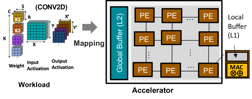
Figure 1. A typical layer-by-layer execution scheme on a canonical DNN accelerator.

Inter-layer Mapping: Layer Fusion. Inter-layer mapping (layer fusion) is an orthogonal map-space to intra-layer mapping. It decides a special tiling dimension across multiple dependent DNN layers. The layer fusion map-space grows exponentially with the number of layers in a DNN workload. For example, if we allow 64 tiling choices per layer (which we use in our evaluations), for an 18 layers DNNs such as Resnet18 (He et al., 2016), the map-space will become as large as $64^{18}$=$O(10^{32})$. With deeper DNN workloads such as Resnet50, Mobilenet-V2, and Mnasnet, the map-space grows to the order of $O(10^{90})$. In this map-space, prior works introduced manually-tuned fusion strategies (Alwani et al., 2016; Wei et al., 2018; Kao et al., 2021), and no prior mappers, to the best of our knowledge, search this space automatically.

3. Problem Formulation

In the DNN accelerator, the on-chip buffer is often limited and not able to stage the full output activation. The key idea of layer fusion is that, rather than streaming back the full output activation to the off-chip memory like in  (Kao et al., 2020b; Hegde et al., 2021; Huang et al., 2021), we stage “partia” output activation on-chip to exploit data locality and thus boost data reuse.

Practitioners start to use “micro-batching” as the go-to strategy. With micro-batching, we will divide a batch of activations into multiple micro-batches. In practice, We search for the largest acceptable micro-batch size that allows us to stage all intermediate activations on-chip, which becomes the most naive micro-batching strategy. However, this naive strategy cannot maximize the reuse opportunity. Different layers produce different sizes of output activations, and a naive unified micro-batch size could leave the on-chip buffer under-utilized.

A more sophisticated layer-wise micro-batching strategy is needed to maximize the on-chip buffer utilization, minimize off-chip access, and finally improve the runtime (latency or throughput) performance.

We call a layer-wise micro-batching strategy — layer fusion strategy, since it is essentially dividing DNN layers into multiple fused-layers. For example, in Fig. 2 we have a layer fusion strategy for a 5-layer DNN workload. The strategy dictates the output micro-batch sizes of each layer, where the first value represents the input micro-batch size. We use ”-1” to represent a signal to synchronize and stream data back to off-chip memory before proceeding to the next layer. This synchronization divides the dataflow into two groups of fused-layers, as shown in Fig. 2(b). The groups of fused-layers will be executed sequentially, as shown in Fig. 2(c). Fig. 2(a) shows a snapshot when the accelerator is executing fused-layer group-0. For an N layer DNN workload, the layer fusion strategy is represented as follows

(2) $$\begin{gathered}Strategy=[mB_{0},mB_{1},...mB_{N}]\end{gathered}$$

, where $mB_{i}$ is the micro-batch size of layer i. To search for the optimum the micro-batching (layer-fusion) strategy, the problem formulation is as follows:

Problem formulation: Given a DNN workload, batch size, and available on-chip memory, produce a layer-fusion strategy that optimizes the end-to-end latency or throughput performance.

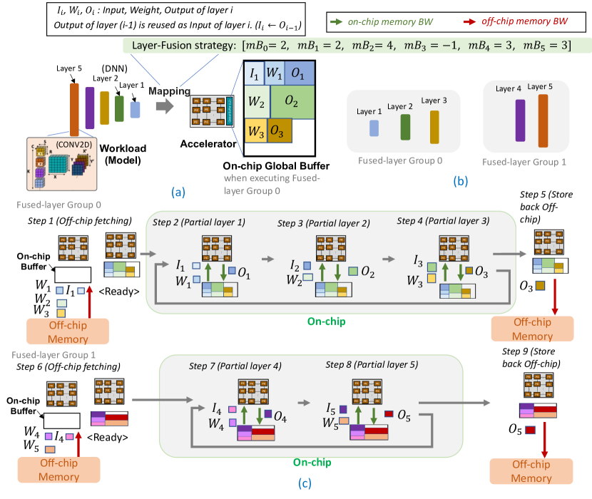
Figure 2. A layer-fusion mapping example on a 5-layer DNN model. (a) The hardware implication, (b) the introduced two group of fused-layer, and (c) the execution steps of each group.

4. DNNFuser

We propose DNNFuser, a pre-trained Transformer-based mapper for layer fusion optimization for DNN workloads. DNNFuser, with a fully trained model, features the ability to infer an optimized mapping for different HW conditions at inference time. As shown in Fig. 3, DNNFuser takes in the input of a workload (a DNN model and its batch size), HW parameters (number of PEs, on-chip BW, off-chip BW), and an HW condition (requesting on-chip buffer usage), and outputs an optimized mapping.

4.1. Motivation for using RLs and Transformers

The key objective is to train a generative model (a decoder model, or a encoder-decoder model where encoder can take in the condition) so that it can serve as a mapper while not incurring any search process. DNNs have been proven repeatedly to have some amount of “knowledge generalization” ability. Deep RLs (DRLs) become one of the best testimonies of this “generalizability”. Even though the number of possible frames (or states) in RL environments, such as Atari games and OpenAI gyms, is often too large to be fully enumerated (similar challenge as in our layer fusion map-space), a well-trained DRL can play well in those environments and generalize its knowledge to states never seen before. This motivates us to take advantage of DRL in our layer fusion problem.

However, DRLs are also known for their “unstableness”, as they rely on NNs to learn the “connection” of each state itself in a long trajectory while also suffering from the delayed reward and vanishing gradient problems (which is even more challenging in our layer fusion problem (discussed in detail in Section 4.4.1)), and are also sensitive to the case-by-case setting of discount rate (Chen et al., 2021). Transformers, meanwhile, are known for their powerful ability to make customized “connections” by attention mechanisms (Vaswani et al., 2017) even in long-sequence scenarios. Recent research (Chen et al., 2021; Boustati et al., 2021; Ortega et al., 2021) shows that learning RL problems with a Transformer is promising and “stable” because it can automatically learn how to attend to previous states and also avoid the discount rate problem.

Therefore, we decide to formulate layer fusion into an RL problem for the potential “generalizability” and utilize Transformers to learn the formulated RL problem for its “stability”.

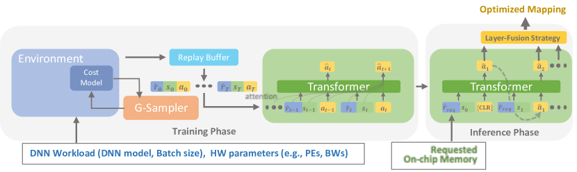
Figure 3. The workflow of DNNFuser.

4.2. Formulating Layer Fusion into RL Problem

We model a micro-batching decision for a layer in the DNN workload as one time-step in the RL environment. For an N layers DNN, the agent (DNNFuser) would go through N+1 time-steps, visiting N+1 states, making N+1 actions, and receiving N+1 rewards, before it receives a “done” signal and complete one trajectory.

Action. The action at time-step t is the micro-batch size of layer-t ($mb_{t}$), also note as $a_{t}$(=$mb_{t}$).

State. We formulate a state at time-step t as follow,

(4) $$\begin{gathered}s_{t}=[K_{t},C_{t},Y_{t},X_{t},R_{t},S_{t},\widehat{M},P_{a_{0}..a_{t-1}}]\end{gathered}$$

The first 6 dimensions are the tensor shape of the current DNN layer. We use the 6-loop notation of CONV layer (other types of layers can also be mapped and represented with these 6-loop notations). $K_{t}$, $C_{t}$ are output and input channels. $Y_{t}$, $X_{t}$ are height and width of activations. $R_{t}$, $S_{t}$ are height and width of weight kernels. $\widehat{M}$ is given as the currently available memory (normalized by the batch size). $P_{a_{0}..a_{t-1}}$ designates the runtime performance (latency or throughput) after a series of actions: [$a_{0}$, …, $a_{t-1}$]. For example at time-step-0, where no previous actions have been made, $P_{0}$ will be the runtime performance before any layer fusion strategy is performed. At time-step-1, $P_{a_{0}}$ is the runtime performance when we only apply layer fusion strategy to the first layer, and so on.

4.3. Transformers for RL-based Layer-Fusion Problem

Reinforcement learning is often noted as harder to converge, higher variance in the result, and unstable in training. Thus, there remains a long-lasting hope of converting RL into a supervised learning problem. Recently, an array of works (Chen et al., 2021; Boustati et al., 2021; Ortega et al., 2021) leverage Transformers to model off-line reinforcement learning and achieve SOTA performance in many typical RL tasks. Leveraging similar taxonomy, we convert our RL-based layer fusion formulation into a Transformer-based supervised learning problem as follows.

4.3.1. Formulation

We convert RL state transition into a sequence like a sentence in language models (similar to  (Chen et al., 2021; Boustati et al., 2021; Ortega et al., 2021)). One trajectory of state transition is a sequence of reward, state, action pair, ([($\widehat{r_{0}}$,$s_{0}$,$a_{0}$), …, ($\widehat{r_{t}}$,$s_{t}$,$a_{t}$), .., ($\widehat{r_{N}}$,$s_{N}$,$a_{N}$)), with N being the number of layers of the targeting DNN models. The Transformer will take this sequence as input and generate a prediction for the next action, $\widehat{a}$, as shown in Fig. 3. For supervised learning, the loss is taken as the Mean Square Error between the predicted action, $\widehat{a_{t}}$, and the actual action, $a_{t}$, for $t\in\mathopen{[}0,1,...,N\mathclose{]}$.

4.3.2. Discussion

There is two high-level intuition for why this formulation is specifically useful in our problem.

• 1) Sparse and distant reward. The correlation between action and reward is often sparse and distant in the layer fusion scenario. The optimal micro-batch and the corresponding impact on the overall memory usage for the current layer often do not depend closely on the last action (last micro-batch decision), but those several time-steps back. The transformer is expected to efficiently deal with the long-sequence scenario and excavate the relation between each action pair, near and far.

• 2) The attention layer in the Transformer is capable of finding shortcuts between individual trajectories (Chen et al., 2021). This means that our DNNFuser can find paths that are missing from the dataset, and more specific to our layer-fusion scenario, some peak memory usages that it has never seen.

4.3.3. Conditional Reward

Rather than the common practice of taking only state or state-action pairs to generate a policy in traditional RLs (Mnih et al., 2016; Lillicrap et al., 2015), we take the full reward-state-action pair as inputs as previously described. The benefit is that the reward is now exposed as input at the inference phase Fig. 3), which opens the opportunity to control the output (mapping solution) by the “desired” reward. This technique is also leveraged in  (Chen et al., 2021).

We use “requesting/conditioning on-chip memory usage” as the conditioning (desired) reward (noted as $\widehat{r_{t}}$). This formulation brings three benefits:

• 1) The current available on-chip memory sizes are known parameters, therefore we could use it as a reasonable condition.

• 2) The heuristics tell that a layer fusion strategy that maximizes the on-chip memory usage often achieves better runtime performance. Therefore, we can expect a high-performance solution if conditioning on the total available memory.

• 3) By setting memory usage as a condition, it also set up a potential use case of generalizing to unseen memory sizes, discussed later in Section 4.6.

4.4. Training Data Collections

4.4.1. Imitation Learning and Teacher Model

An DNN learning trick, “imitation learning”, is found useful in training Transformers (Chen et al., 2021; Boustati et al., 2021; Ortega et al., 2021). “Imitation learning” could be imitating and learning 1) from self previous experiences as used in related works (Chen et al., 2021; Boustati et al., 2021; Ortega et al., 2021) or 2) from another well-trained teacher model, which we use in this work and find it critical for Transformers to learn well in our layer fusion problem.

In previous work, such as Decision Transformer (DT) (Chen et al., 2021), the “imitation learning” dataset is collected by an RL agent sampling in the targeting Atari or OpenAI environment. However, we find that popular RL algorithms, including Advantage Actor-Critic (A2C) (Mnih et al., 2016) and Deep Deterministic Policy Gradient (DDPG) (Lillicrap et al., 2015), suffer from inefficient sampling when interacting with the layer fusion map-space, and their trajectories are therefore inefficient demonstrations for “imitation learning”.

We observe that, unlike Atari or OpenAI with smooth state transitions, in our mapping problem, state transits abruptly between two consecutive time-steps (e.g., the state includes information of current layer shape, which does not have deducible relation to the layer shape in next state), and that the variance is detrimental to the convergence of the mentioned RL algorithms. Thus, rather than letting the agent (our model) explore in the environment itself to collect “experiences”, which is particularly inefficient in this case, we decide to use a teacher model, with some prior knowledge, to demonstrate directly some good trajectories. Next, we will discuss the details of our teacher model.

4.4.2. Developed Teacher Model: G-Sampler

Gamma (Kao et al., 2020b) is one of the SOTA intra-layer mappers for DNN accelerators. We extended Gamma to support inter-layer layer-fusion map-space and found it several orders of magnitude better in performance than other optimization methods such as A2C (Mnih et al., 2016), PSO (Kennedy and Eberhart, 1995), DE (Price, 2013), and so on (Hansen, 2006; Hellwig and Beyer, 2016; Pelikan et al., 1999; Lillicrap et al., 2015; Sutton et al., 2000), which we show in our evaluations (Section 5.2). We use the developed extended Gamma as our teach model and call it —G-Sampler. We use G-Sampler to search for optimal layer-fusion strategy given different on-chip buffer sizes.

Note that we empirically found that G-Sampler works well as a layer fusion mapper, which beats many optimization methods. However, G-Sampler is still a search-based method, which is inevitably slower than most of the inference-based DNN models. Therefore, G-Sampler only serves as a training data generator, which samples several good solutions (trajectories) in the layer-fusion environment (Fig. 3). DNNFuser, as a student, learns from these demonstrations and generalizes the knowledge to learn to generate optimized mapping at inference time.

4.5. Model Training and Inference

4.5.1. Training

With all the above-mentioned preparation and setup, we can now train our model. As shown in Fig. 3, the steps are as follows. 1) Data collection with teacher model. We take G-Sampler and ask it to search for several (4-10) sets of optimized mapping in different conditions (on-chip memory sizes). 2) Formulating into RL state transition. We take those solutions, which is a sequence of actions in RL terminology, and decorate them with the state and reward information to make it a state transition trajectory. These decorated trajectories will be stored in the replay buffer (essentially a place to house the training dataset). 3) Model training. We sample the training data from the replay buffer and train our model in an ”imitation learning” fashion.

4.5.2. Inference

At inference time, the model takes in a conditioning reward, which is the conditioning on-chip buffer usage, and generates a sequence of actions as a solution in an auto-regressive manner. The actual on-chip buffer usage of the solution adheres to the desired condition.

4.6. Generalization and Transfer Learning

4.6.1. Generalization

After training, DNNFuser can work on not only the seen conditions (on-chip buffer sizes) but also some unseen conditions. For example, we can train DNNFuser with some conditioning on-chip buffer sizes, such as 16, 32, 48, and 64 MB, and it could generalize its knowledge to the unseen interpolated buffer sizes between 16-64MB. For example, if the available buffer sizes in the HW suddenly change from 32MB to 28MB because some amount of buffer is occupied by other small procedures. We do not need to re-train the model (or launch a new search as we will need in a traditional search-based method). We can simply do another inference with 28MB as the new condition, and DNNFuser with its generalized knowledge could infer a solution.

4.6.2. Transfer Learning

DNNFuser can be trained on one or several common DNN workloads and serve as a pre-trained model for transfer learning. For a new DNN workload, we can take this general model and fine-tune it on the new workload. The fine-tuning process only takes a few epochs to converge since the generalized knowledge in DNNFuser can be transferred and utilized in the new workload. Empirically, we find that fine-tuning process requires only 10% of the training epoch compared to training from scratches, and can achieve compatible or better performance than a training-from-scratch model.

5. Evaluation

5.1. Setup

Workload. We experiment on several common DNN workloads, including VGG16 (Simonyan and Zisserman, 2014), Resnet18 (He et al., 2016), Resnet50 (He et al., 2016), Mnasnet (Tan et al., 2019), and Mobilenet-V2 (Sandler et al., 2018).

Accelerator Assumption. We experiment on the DNN accelerator configurations of 1024 PEs, on-chip buffer sizes of 64 MB, off-chip memory BW of 900GB/s, on-chip memory BW of 9000GB/s, and frequency of 1GHz, which is similar to  (Jouppi et al., 2020; Chen et al., 2016). We set this as our underlying DNN accelerator modeled by our cost model.

Cost Model. We built an analytical cost model to model the effect of layer fusion in DNN accelerators. The cost model focuses on modeling interactions between layers and assumes the ideal performance for intra-layer map-space, which can already be achieved by existing intra-layer mappers (Hegde et al., 2021; Kao et al., 2020b). The cost model takes in a DNN workload, the number of PEs, on-chip memory size, on-chip and off-chip memory bandwidths (BW), and a layer fusion strategy, and returns its runtime performance and peak memory usage. The built cost model is validated against MAESTRO (Kwon et al., 2018), which is in turn validated again real chip performance.

Baseline Mapping. Our baseline mapping, no-fusion mapping, is the best possible mapping without exploring layer fusion map-space (i.e., the most ideal mapping in intra-layer map-space), representing mapping that can be found by existing SOTA mappers (Kao et al., 2020b; Hegde et al., 2021; Huang et al., 2021). To compare the effectiveness of the different searching algorithms for this fusion strategy search problem, we compute the speedup of the solution proposed by each searching algorithm (a fusion-based mapping) to the baseline mapping (no-fusion mapping).

Baseline Search Methods. Among optimization methods, we compare with many widely used ones as our baseline search methods for the inter-layer mapping, including Particle Swarm Optimization (PSO), Covariance matrix adaptation evolution strategy (CMA-ES), Differential Evolution (DE), Test-based population-size adaptation (TBPSA) and standard GA (stdGA), whose implementations are from nevergrad (Rapin and Teytaud, 2018) by Facebook. We also implement an RL method A2C (Mnih et al., 2016). We allow all of them to have sampling budgets of 2K.

Baseline Sequence Model. DNNFuser is a Transformer-based sequence models. To show the effectiveness of Transformer as the sequence model for this problem, We also implement an RNN-based sequence-to-sequence model (Seq2Seq) as a baseline sequence model. The Seq2Seq is made of a LSTM with 2 layers of fully connected layers and 128 hidden dimension in each encoder and decoder.

Performance Metric. To fairly compare the effectiveness of optimization methods, we compare the achieved speedup of their layer-fusion solutions over the baseline mapping.

Implementation Details of G-Sampler. G-Sampler, our developed search method (Section 4.4.2), has a population size of 40 and runs for 50 generations, which also ends at a sampling budget of 2K as baselines do.

Implementation Detail of DNNFuser. DNNFuser is made of three transformer blocks, two heads, and a hidden dimension size of 128. We train the model for 100K epochs.

Table 1. Performance comparisons of different optimization methods on VGG16 workload with two different cases of on-chip memory constraints. The speedup is the latency of the found mapping by each search algorithm to the latency of the baseline mapping (described in Section 5.1.) All the experiments run on a 4-core Intel Xeon CPU with a Nvidia GTX 1070 GPU.

Algorithm	Speedup	Act. Usage (MB)	Search Time (mins)
Case-1	On-chip Memory constraint 20M, Batch size 64
PSO	N/A	102.76	69.17
CMA	N/A	186.25	77.03
DE	N/A	114	65.17
TBPSA	N/A	153.34	110.50
stdGA	N/A	139.69	61.66
A2C	0.98	2.26	335.63
G-Sampler	1.19	16.46	0.66
Seq2Seq	1.05	16.06	0.01
DNNFuser	1.20	19.27	0.01
Case-2	On-chip Memory constraint 40M, Batch size 128
PSO	N/A	255.3	93.28
CMA	N/A	411.04	91.42
DE	N/A	149.32	104.74
TBPSA	N/A	245.66	106.20
stdGA	N/A	236.03	151.74
A2C	N/A	372.51	293.81
G-Sampler	2.06	37.73	1.27
Seq2Seq	1.51	35.4	0.01
DNNFuser	3.13	37.73	0.01

Table 2. Speedup performance of DNNFuser (DF) and Seq2Seq (S2S) on unseen conditioning memory usage (20, 25, 40, 35, 40, and 45MB). DNNFuser is only trained on conditioning memory usage of 16, 32, 48, and 64MB.

Model (Batch=64)	VGG16			Resnet18
Cond. Mem. Usage (MB)	DF	S2S	G- Sampler	DF	S2S	G- Sampler
20	1.20	1.04	1.19	1.27	1.32	1.37
25	1.20	1.04	2.18	1.27	1.32	1.34
30	1.16	1.83	1.86	2.31	1.56	1.51
35	1.88	1.85	2.14	2.31	1.56	1.53
40	1.97	1.86	2.17	2.68	1.56	2.88
45	1.97	2.02	2.30	2.68	1.56	2.95

Table 3. Speedup comparisons of Transfer-DF (DNNFuser pre-trained on VGG16 and Resnet18 and tranfer learning on new workloads), Direct-DF (DNNFuser trained from scratch on new workload), and GS (G-Sampler running full-search) on different conditioning memory usage.

Cond. Mem. Usage (MB)	Transfer-DF	Direct-DF	GS
	Resnet50, Batch size 64
25	1.31	1.17	1.41
35	1.78	1.78	1.94
45	2.01	2.03	2.13
55	2.55	2.03	2.26
	Mobilenet-V2, Batch size 64
25	1.83	1.68	2.27
35	2.01	1.67	2.18
45	2.66	2.90	2.41
55	2.94	N/A	4.32
	Mnasnet, Batch size 64
25	3.34	N/A	3.60
35	3.34	3.34	3.17
45	3.34	3.34	3.82
55	3.46	3.53	4.07

5.2. Comparisons with Baselines

First of all, the sampling efficiency of the optimization algorithms will decide the quality of the found solutions. In this experiment, the constraint is the on-chip memory usage, and the objective is to minimize the latency. Many baseline methods such as PSO, CMA, DE, and so on, cannot meet the on-chip memory usage constraint. Note that their memory usage is larger than 20MB (or 40MB at the bottom half the table) in Table 1. Therefore their solution is invalid, and we mark the invalid solution as N/A. They cannot find valid solution within the given 2K sampling budget. Given “enough” sampling budget, they will eventually learn the constraint and start to optimize the latency. However, 2K sampling budget already take them 1-2 hours. The need of more sampling budget and more hours make these baseline methods not ideal for this problem.

A2C can successfully find a valid solution within the sampling budget. However, it takes around 5 hours, and its solution ends up worse than the baseline mapping, i.e., speedup smaller than 1.0.

Next we discuss the choice of sequence model in our framework, it could be the Transformer-based DNNFuser or an RNN-based Seq2Seq model. For both sequence models, we leverage the G-Sampler to generate the examples (training data for the sequence models). G-Sampler itself can converge within around 1.3 mins and achieve 1.19x and 2.06x speedup over the baseline mapping. As for the sequence model, we could observe that both DNNFuser and Seq2Seq can perform well in our framework in terms of search time and achieved speedup. However, DNNFuser can constantly find better solution, achieving more speedup than Seq2Seq. DNNFuser takes around 0.6-1.3 mins for searching and achieves 1.19x and 2.06x speedup over the baseline mapping. DNNFuser can find the solution with compatible or better performance than G-Sampler and is 66x-127x faster than it.

5.3. Generalizing to Unseen HW Condition

We train DNNFuser on VGG16 and Resnet18 respectively, using the memory condition of on-chip memory usages of 16, 32, 48, and 64MB. Without re-training, DNNFuser can directly generalize its knowledge to unseen HW conditions and infer corresponding solutions, the memory condition of 20, 25, 30, 35, 40, and 45, as shown in Table 2. Note that all of these conditions are unseen for the trained DNNFuser, and they are the interpolation of the range of memory condition (16 - 64MB) that DNNFuser is trained on. With only one inference, DNNFuser and Seq2Seq can both find solutions with compatible performance to G-Sampler while G-Sampler is running full-search. Among DNNFuser and Seq2Seq, we can observe their performance is compatible on VGG16. However, on Resnet18 DNNFuser is a clear win. It is because Resnet18 with more number of layers than VGG16 forms a longer sequence, and DNNFuser (a Transformer-based model) performs better than Seq2Seq (a RNN-based model) at longer sequence tasks.

5.4. Transfer Learning

To demonstrate the ability to execute transfer learning, we train DNNFuser on both VGG16 and Resnet18 to form a pre-trained general model. Then we use this general model to execute transfer learning on new DNN workloads: Resnet50, Mobilenet-V2, and Mnasnet. We fine-tune on new workloads (Transfer-DFs) with only 10% of the training epochs compared to training-from-scratch (Direct-DFs). As shown in Table 3, with only 10% of training epochs, Transfer-DFs can achieve compatible performance with G-Sampler and better performance than Direct-DFs (looking at some edge cases where Direct-DFs fail (N/A)). This tells that prior knowledge gained from pre-training actually increases the training speed and quality, which is especially important when training large DNN workloads such as Resnet50, Mobilenet-V2, or Mnasnet, which would otherwise require more training data. I.e., Direct-DFs need more teacher demonstrations from the Teacher model than Tranfer-DFs. This observation showcases the usefulness of transfer learning—with a pre-trained general model of DNNFuser, we can learn new workloads faster and better.

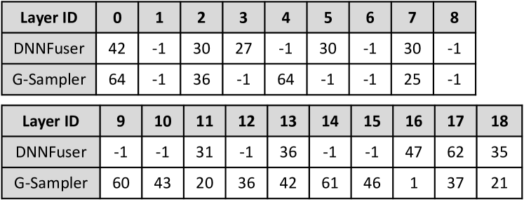
Figure 4. The layer-fusion mapping found by DNNFuser and G-Sampler on ResNet18 with batch size 64 conditioning on memory size of 20MB. Values represent the micro-batch size of each layer, with LayerID 0 being the input to LayerID 1.

5.5. Analysis of Found Solutions

In Fig. 4, we show one of the solutions found by DNNFuser and G-Sampler. There are two main observations: 1) at deeper layers, they learn to fuse more number of layers, since deeper layers tend to have smaller activations. 2) Sudden expansion in either channel depth (e.g. layer 6) or activation shape (due to residual connections) (e.g. layer 8) propels them to synchronize back off-chip because staging on-chip puts too much pressure on the memory capacity.

6. Related Work

DNN Mapper. There are many DNN mapper proposals utilizing different optimization methods, such as simulated annealing in TVM (Chen et al., 2018), RL in FlexTensor (Zheng et al., 2020) and ConfuciuX (Kao et al., 2020a), Mixed Integer Programming in CoSA (Huang et al., 2021), domain-specific GA in GAMMA (Kao et al., 2020b), gradient-based surrogate model in MindMapping (Hegde et al., 2021), and many others. However, 1) all the previously mentioned prior arts are mappers for intra-layer map-space while DNNFuser is a mapper for the less explored inter-layer map-space, and 2) they are search-based methods while DNNFuser is an inference-based method.

Layer-Fusion. Some compiler works also study ”Operator-Fusion” such as  (Ivanov et al., 2020; Niu et al., 2021), however, we want to clarify that ”Operator-Fusion” usually fuses CONV or MatMul layer with element-wise operators such as ReLU but not several CONVs, FCs, or MatMul as we refer to by ”Layer-Fusion”. ”Layer-Fusion” has more complexity and is therefore often discussed in the context of inter-layer dataflow or mapping. Layer fusion is an orthogonal map-space to intra-layer mapping where most DNN mapper focuses on. Some recent works have looked into this map-space such as fused-layer CNN (Alwani et al., 2016), TGPA (Wei et al., 2018), and FLAT (Kao et al., 2021) and demonstrate the huge potential performance improvement by leveraging this one additional mapping dimension in DNN mapping. However, the previously mentioned prior arts focus on proposing a hand-tuned layer fusion strategy for the considered use-cases. In contrast, DNNFuser is a mapper which can work on different use-cases automatically.

Transformers for RL Problems. Adapting RLs as sequence modeling problems has not been notably successful until some recent works, such as Decision Transformer (Chen et al., 2021). Further applications showcase its vitality. Boustati et. al. (Boustati et al., 2021) examined and discovered some significant potentials in transfer learning, and (Ortega et al., 2021) by DeepMind developed the idea further to human-AI interaction. This work, to the best of our knowledge, is the first work using a transformer with RL formulation to tackle DNN mapping problem.

7. Conclusion

We propose a mapper, DNNFuser, for Layer-Fusion map-space, featuring its ability to find a solution at inference time, much faster compared to the best existing search-based mappers with compatible performance. DNNFuser can also generalize to unseen conditions and do transfer learning on a new DNN workload.

References

- (1)
- Alwani et al. (2016) M. Alwani et al. 2016. Fused-layer CNN accelerators. In MICRO. IEEE, 1–12.
- Boustati et al. (2021) Ayman Boustati et al. 2021. Transfer learning with causal counterfactual reasoning in Decision Transformers. arXiv:2110.14355 [cs.LG]
- Chen et al. (2021) Lili Chen et al. 2021. Decision transformer: Reinforcement learning via sequence modeling. arXiv preprint arXiv:2106.01345 (2021).
- Chen et al. (2018) Tianqi Chen et al. 2018. Learning to optimize tensor programs. In NeurIPS. 3389–3400.
- Chen et al. (2016) Yu-Hsin Chen et al. 2016. Eyeriss: A spatial architecture for energy-efficient dataflow for convolutional neural networks. In ISCA.
- Google (2020) Google. 2020. Edge TPU. https://cloud.google.com/edge-tpu
- Hansen (2006) Nikolaus Hansen. 2006. The CMA evolution strategy: a comparing review. In Towards a new evolutionary computation. Springer, 75–102.
- He et al. (2016) Kaiming He et al. 2016. Deep residual learning for image recognition. In CVPR. 770–778.
- Hegde et al. (2021) Kartik Hegde, Po-An Tsai, Sitao Huang, Vikas Chandra, Angshuman Parashar, and Christopher W Fletcher. 2021. Mind mappings: enabling efficient algorithm-accelerator mapping space search. In Proceedings of the 26th ACM International Conference on Architectural Support for Programming Languages and Operating Systems. 943–958.
- Hellwig and Beyer (2016) Michael Hellwig and Hans-Georg Beyer. 2016. Evolution under strong noise: A self-adaptive evolution strategy can reach the lower performance bound-the pccmsa-es. In International Conference on Parallel Problem Solving from Nature. Springer, 26–36.
- Huang et al. (2021) Qijing Huang et al. 2021. CoSA: Scheduling by Constrained Optimization for Spatial Accelerators. arXiv preprint arXiv:2105.01898 (2021).
- Ivanov et al. (2020) Andrei Ivanov et al. 2020. Data Movement Is All You Need: A Case Study on Optimizing Transformers. arXiv e-prints (2020), arXiv–2007.
- Jouppi et al. (2020) Norman P. Jouppi, Doe Hyun Yoon, George Kurian, Sheng Li, Nishant Patil, James Laudon, Cliff Young, and David Patterson. 2020. A Domain-Specific Supercomputer for Training Deep Neural Networks. Commun. ACM 63, 7 (June 2020), 67–78. https://doi.org/10.1145/3360307
- Kao et al. (2020a) Sheng-Chun Kao et al. 2020a. ConfuciuX: Autonomous Hardware Resource Assignment for DNN Accelerators using Reinforcement Learning. In MICRO. IEEE, 1–14.
- Kao et al. (2020b) Sheng-Chun Kao et al. 2020b. GAMMA: Automating the HW mapping of DNN models on accelerators via genetic algorithm. In ICCAD. IEEE, 1–9.
- Kao et al. (2021) Sheng-Chun Kao et al. 2021. An Optimized Dataflow for Mitigating Attention Performance Bottlenecks. arXiv preprint arXiv:2107.06419 (2021).
- Kennedy and Eberhart (1995) James Kennedy and Russell Eberhart. 1995. Particle swarm optimization. In Proceedings of ICNN’95-International Conference on Neural Networks, Vol. 4. IEEE, 1942–1948.
- Kwon et al. (2018) Hyoukjun Kwon, Michael Pellauer, and Tushar Krishna. 2018. An Analytic Model for Cost-Benefit Analysis of Dataflows in DNN Accelerators. arXiv preprint arXiv:1805.02566 (2018).
- Lillicrap et al. (2015) Timothy P Lillicrap et al. 2015. Continuous control with deep reinforcement learning. arXiv preprint arXiv:1509.02971 (2015).
- Mnih et al. (2016) Volodymyr Mnih et al. 2016. Asynchronous methods for deep reinforcement learning. In ICML. 1928–1937.
- Niu et al. (2021) Wei Niu et al. 2021. DNNFusion: accelerating deep neural networks execution with advanced operator fusion. In PLDI’21. 883–898.
- NVIDIA (2018) NVIDIA. 2018. NVIDIA Deep Learning Accelerator (NVDLA). https://nvldla.org.
- Ortega et al. (2021) Pedro A. Ortega et al. 2021. Shaking the foundations: delusions in sequence models for interaction and control. arXiv:2110.10819 [cs.LG]
- Pelikan et al. (1999) Martin Pelikan et al. 1999. BOA: The Bayesian optimization algorithm. In Proceedings of the genetic and evolutionary computation conference GECCO-99, Vol. 1. 525–532.
- Price (2013) Kenneth V Price. 2013. Differential evolution. In Handbook of Optimization. Springer, 187–214.
- Rapin and Teytaud (2018) J. Rapin and O. Teytaud. 2018. Nevergrad - A gradient-free optimization platform. https://GitHub.com/FacebookResearch/Nevergrad.
- Sandler et al. (2018) Mark Sandler, Andrew Howard, Menglong Zhu, Andrey Zhmoginov, and Liang-Chieh Chen. 2018. Mobilenetv2: Inverted residuals and linear bottlenecks. In Proceedings of the IEEE Conference on Computer Vision and Pattern Recognition. 4510–4520.
- Simonyan and Zisserman (2014) Karen Simonyan and Andrew Zisserman. 2014. Very deep convolutional networks for large-scale image recognition. arXiv preprint arXiv:1409.1556 (2014).
- Sutton et al. (2000) Richard S Sutton et al. 2000. Policy gradient methods for reinforcement learning with function approximation. In Advances in neural information processing systems. 1057–1063.
- Tan et al. (2019) Mingxing Tan, Bo Chen, Ruoming Pang, Vijay Vasudevan, Mark Sandler, Andrew Howard, and Quoc V Le. 2019. Mnasnet: Platform-aware neural architecture search for mobile. In Proceedings of the IEEE Conference on Computer Vision and Pattern Recognition. 2820–2828.
- Vaswani et al. (2017) Ashish Vaswani et al. 2017. Attention is all you need. In NeurIPS. 5998–6008.
- Wei et al. (2018) Xuechao Wei et al. 2018. TGPA: tile-grained pipeline architecture for low latency CNN inference. In ICCAD. 1–8.
- Xiao et al. (2021) Qingcheng Xiao et al. 2021. HASCO: Towards Agile HArdware and Software CO-design for Tensor Computation. arXiv preprint arXiv:2105.01585 (2021).
- Zheng et al. (2020) Size Zheng et al. 2020. Flextensor: An automatic schedule exploration and optimization framework for tensor computation on heterogeneous system. In ASPLOS’20. 859–873.