A dual approach for federated learning

Abstract

We study the federated optimization problem from a dual perspective and propose a new algorithm termed federated dual coordinate descent (FedDCD), which is based on a type of coordinate descent method developed by Necora et al. [Journal of Optimization Theory and Applications, 2017]. Additionally, we enhance the FedDCD method with inexact gradient oracles and Nesterov’s acceleration. We demonstrate theoretically that our proposed approach achieves better convergence rates than the state-of-the-art primal federated optimization algorithms under certain situations. Numerical experiments on real-world datasets support our analysis.

1 Introduction

With the development of artificial intelligence, people recognize that many powerful machine learning models are driven by large distributed datasets, e.g., AlphaGo [Silver et al., 2016] and AlexNet [Krizhevsky et al., 2012]. In many industrial scenarios, training data are maintained by different organizations, and transporting or sharing the data across these organizations is not feasible because of regulatory and privacy considerations [Li et al., 2020a]. Therefore there is increasing interest in training machine learning models that operate without gathering all data in a single place. Federated learning (FL), initially proposed by McMahan et al. [2017] to train models on decentralized data from mobile devices, and later extended by Yang et al. [2019] and Kairouz et al. [2019], is a training framework that allows multiple clients to collaboratively train a model without sharing data.

The learning process in FL can be formulated as a distributed optimization problem, which is also known as federated optimization (FO). Assume there are $N$ clients and each client $i$ maintains a local dataset $\mathcal{D}_{i}$. FO aims to solve the empirical-risk minimization problem

$$\mathop{\hbox{minimize}}_{w\in\mathbb{R}^{d}}\enspace F(w)\coloneqq\sum_{i=1}^{N}f_{i}(w)$$ (P)

in a distributed manner, where $w$ is the global model parameter and each local objective $f_{i}:\mathbb{R}^{d}\to\mathbb{R}$ is defined by

$$f_{i}(w)=\ell(w;\mathcal{D}_{i}),$$

where $\ell(\cdot,\mathcal{D}_{i})$ is a convex and differentiable loss function for each $\mathcal{D}_{i}$.

As characterized and formalized by Wang et al. [2021], Li et al. [2020b] and Li et al. [2020d], there are several important characteristics that distinguish FO from standard machine learning and distributed optimization.

Assumption 1.1 (Governing assumptions).

The following assumptions hold for FO.

• Slow Communication. Communication between clients and a central server is assumed to be the main bottleneck and dominates any computational work done at each of the clients.

• Data Privacy. Clients want to keep their local data private, i.e., their data can not be accessed by any other client nor by the central server.

• Data heterogeneity. The training data are not independent and identically distributed (i.i.d.). In other words, a client’s local data cannot be regarded as samples drawn from single overall distribution.

• Partial Participation. Unlike traditional distributed learning systems, an FL system does not have control over individual client devices, and clients may have limited availability for connection.

Most of the previous work in FO focus on directly solving the primal empirical-risk minimization problem (P) [McMahan et al., 2017; Li et al., 2020c; Yuan et al., 2021; Karimireddy et al., 2021]. The broad approach taken by these FO proposals is based on requiring the clients to independently update local models that are then shared with a central server tasked with aggregating these models.

Dual approaches for empirical-risk minimization problem (P) are well developed under the framework of distributed optimization, and can be traced to dual-decomposition [Zeng et al., 2008; Joachims, 1999], augmented Lagrangian  [Jakovetić et al., 2014] and alternating direction method of multipliers (ADMM) [Boyd et al., 2011; Wei and Ozdaglar, 2012]. More recent approaches include ingel-step and multi-step dual accelerated (SSDA and MSDA) methods [Scaman et al., 2017]. These methods, however, can not be directly applied under the FO setting, because they violate some of Assumption 1.1. For example, the MSDA algorithm [Scaman et al., 2017] enjoy optimal convergence rates, but requires full clients participation in every round, which is unrealistic under Assumption 1.1.

Our approach, in contrast, is based on the dual problem, which is a separable optimization problem with a structured linear constraint (D). We show that the random block coordinate descent method for problems with linear constraint proposed by Necoara et al. [2017], is especially suitable for the FL setting. Because it is important to control the amount of local computation carried out by each client, we show how to modify this method to accommodate inexact gradient oracles. We also show how Nesterov’s acceleration can be used to decrease overall complexity. As a result, we obtain convergence rates that are better than other state-of-the-art FO algorithms in certain scenarios.

Our contributions can be summarized as follows.

1. We tackle the FO problem from a dual perspective and develop a federated dual coordinate descent (FedDCD) algorithm for FO based on the random block coordinate descent (RBCD) method proposed by Necoara et al. [2017]. We show that FedDCD fits very well to the settings of FL.

2. We extend the FedDCD with inexact gradient oracles and Nesterov’s acceleration. The resulting convergence rates are better than the current state-of-the-art FO algorithms in certain situations.

3. We develop a complexity lower bound for FO, the lower bound suggests that there is still a gap of $\sqrt{N}$ between the rate of accelerated FedDCD and the lower bound.

2 Related work

Distributed and parallel optimization has been extensively studied starting with the pioneering work from Bertsekas and Tsitsiklis [1989]. In addition to the previous mentioned ADMM, SSD and MSDA methods, popular distributed optimization algorithms include randomized gossip algorithms [Boyd et al., 2006] and various distributed first-order methods such as the distributed gradient descent [Nedic and Ozdaglar, 2009], distributed dual averaging [Duchi et al., 2012], distributed coordinate descent [Richtárik and Takác, 2016], and EXTRA [Shi et al., 2015].

Federated optimization [Wang et al., 2021] is a newly emerged research subject that is closely related to centralized distributed optimization. However, most existing distributed optimization algorithms cannot be directly applied to FO because of Assumption 1.1. Because FL problems usually involve a large number of total data points, most existing FO algorithms for solving (P) such as mini-batch SGD (MB-SGD) [Woodworth et al., 2020], FedAvg (aka. local SGD) [McMahan, 2017], FedProx [Li et al., 2020c], FedDualAvg [Yuan et al., 2021], SCAFFOLD [Karimireddy et al., 2020], MIME [Karimireddy et al., 2021] are variants of the SGD algorithm. Methods outside of the SGD framework are not as well developed.

The method we develop is based on a variation of coordinate descent adapted to problems with structured linear constraints. Such algorithms have been well-studied in the context of kernel support vector machine (SVM) [Luo and Tseng, 1993; Platt, 1998; Chang and Lin, 2011]. We build on the method proposed by Necoara et al. [2017].

3 Problem formulation

The dual problem of problem (P) is given by

$$\mathop{\hbox{minimize}}_{y_{1},\dots,y_{N}\in\mathbb{R}^{d}}\enspace G(y)\coloneqq\sum_{i=1}^{N}f_{i}^{*}(y_{i})\enspace\mathop{\hbox{subject to}}\enspace\sum_{i=1}^{N}y_{i}=0,$$ (D)

where $f_{i}^{*}(y)\coloneqq\sup_{w}\langle y,w\rangle-f(w)$ is the convex conjugate function of $f_{i}$. Throughout this paper, we denote $y^{*}$ as a solution of problem (D). To obtain this dual problem let $w^{*}$ denote the optimal solution to the primal problem eq. P. By the first-order optimality condition, we know that

$$0\in\partial\left(\sum_{i=1}^{N}f_{i}\right)(w^{*}),$$

which is equivalent to

$$w^{*}\overset{\rm{(i)}}{\in}\partial\left(\sum_{i=1}^{N}f_{i}\right)^{*}(0)\overset{\rm{(ii)}}{=}\partial\left(\mathop{\square}_{i=1}^{N}f_{i}^{*}\right)(0)\overset{\rm{(iii)}}{=}\bigcap_{i=1}^{N}\partial f_{i}^{*}(y_{i}^{*}),$$

where $\{y_{i}^{*}\}_{i=1}^{N}$ are the optimal solutions to the problem (D), and (i), (ii) and (iii), respectively, follow from Hiriart-Urruty and Lemaréchal [2001, Proposition E.1.4.3, Proposition E.2.3.2 and Corollary D.4.5.5].

3.1 Assumptions and notations

We make the following standard assumptions on each of the primal objectives $f_{i}$.

Assumption 3.1 (Strong convexity).

There exist $\alpha>0$ such that

$$f_{i}(x)\geq f_{i}(y)+\langle\nabla f_{i}(y),x-y\rangle+\frac{\alpha}{2}\|x-y\|^{2}$$

for any $x,y\in\mathbb{R}^{d}$ and $\forall i\in[N]$. This also implies that $G$ is $(1/\alpha)$ block-wise smooth.

Assumption 3.2 (Smoothness).

There exist $\beta>0$ such that

$$f_{i}(x)\leq f_{i}(y)+\langle\nabla f_{i}(y),x-y\rangle+\frac{\beta}{2}\|x-y\|^{2}$$

for any $x,y\in\mathbb{R}^{d}$ and $\forall i\in[N]$. This also implies that $G$ is $(1/\beta)$ block-wise strongly convex.

These two assumptions are critical because they yield a one-to-one correspondence between the primal and dual spaces, and allow us to interpret each $y_{i}$ as a local dual representation of the global model $w$.

Our analysis also applies to the case where the parameters $\alpha$ and $\beta$ vary for each function $f_{i}$, but here we assume for simplicity, these are fixed for each $f_{i}$.

The data-heterogeneity between clients can be measured as the diversity of the function $f_{i}$, as measured by the gradient. In the convex case, it is sufficient to measure the diversity of functions only at the optimal point $w^{*}$; see Koloskova et al. [2020, Assumption 3a].

Assumption 3.3 (Data heterogeneity).

Let $w^{*}=\arg\min~{}F(w)$. There exist $\zeta>0$ such that for any $i\in[N]$,

$$\left\|\nabla f_{i}(w^{*})\right\|\leq\zeta.$$

The relationship between $y_{i}^{*}$ and $\nabla f_{i}(w^{*})$ implies that $\|y_{i}^{*}\|\leq\zeta~{}\forall i\in[N]$, where $y^{*}$ is the solution of problem (D).

A basic assumption in FL is that the central server does not have control over clients’ devices and can not guarantee their per-round participation. Partial participation, therefore, is a respected feature for efficient FL. Here we follow the standard random participation model [Wang et al., 2021; Li et al., 2020b, d] and assume that there is a fixed number of randomly generated clients participating in each round of the training.

Assumption 3.4 (Random partial participation).

There exist a positive integer $\tau\in\{2,\dots,N\}$, such that in each round, only $\tau$ clients uniformly randomly distributed among the set of all clients, who can communicate with the central server.

Now we introduce some notations. For any integer $N$, we denote $[N]$ as the set $\{1,2,\ldots,N\}$. Given $I\subseteq[N]$ and $\{g_{i}\in\mathbb{R}^{d}\mid i\in[N]\}$, we define the concatenation $g_{I}\in\mathbb{R}^{Nd}$ as

$$g_{I}[(i-1)d+1:i\cdot d]=\begin{cases}g_{i}&i\in I;\\ 0&\mbox{otherwise}.\end{cases}$$

Given $I\subseteq[N]$, we define the linear manifold

$$\mathcal{C}_{I}=\left\{y\in\mathbb{R}^{Nd}~{}\Bigg{|}~{}y_{i}\in\mathbb{R}^{d},~{}\sum_{i\in I}y_{i}=0\right\}.$$

It follows that $\mathcal{C}_{[N]}$ corresponds to the constraint set in eq. D. Let $e_{d}\in\mathbb{R}^{d}$ denote the vector of all ones, and $e_{I}$ denote vector where $e_{i}=1$ if $i\in I$ and $e_{i}=0$ elsewhere. For any positive definite matrix $W\in\mathbb{R}^{Nd\times Nd}$, we define the weighted norm as $\|x\|_{W}:=\sqrt{x^{T}Wx}$. The projection operator onto the set $\mathcal{C}_{I}$ with respect to the weighted norm $\|\cdot\|_{W}$ is defined as

$$\operatorname{proj}_{\mathcal{C}_{I}}^{W}(x)=\mathop{\hbox{arg\,min}}_{y}\|y-x\|_{W}^{2}\enspace\mathop{\hbox{subject to}}\enspace y\in\mathcal{C}_{I}.$$

4 Federated dual coordinate descent

Necoara et al. [2017] proposed a random block coordinate descent (RBCD) method for solving linearly constrained separable convex problems such as the dual problem (D). Below we describe how to apply this method in the FL setting, and we refer to the specialization of this algorithm as federated dual coordinate descent (FedDCD).

A training round proceeds as follows. In round $t$, suppose that the local dual representations $y_{i}^{(t)}$ are dual feasible, i.e.,

$$\sum_{i=1}^{N}y_{i}^{(t)}=0.$$

First, the central server receives the IDs of participating clients $I=\{i_{1},\dots,i_{\tau}\}\subseteq\{1,\dots,N\}$. Next, each participating client computes a local primal model $w_{i}^{(t)}$, which can also be interpreted as a descent direction for the dual representation, in parallel, i.e.,

$$w_{i}^{(t)}=\nabla f_{i}^{*}(y_{i}^{(t)})=\mathop{\hbox{arg\,min}}_{w\in\mathbb{R}^{d}}\enspace\left\{f_{i}(w)-\langle w,y_{i}^{(t)}\rangle\right\}\text{for all}i\in I.$$ (1)

In principle, each participating client must exactly minimizes $f_{i}-\langle\cdot,y_{i}^{(t)}\rangle$, using a potentially expensive procedure, to obtain $w_{i}^{(t)}$. We show in the next section how the clients may instead produce an approximate primal model $w_{i}^{(t)}$ using a cheaper procedure. Then each participating client sends the computed local primal model $w_{i}^{(t)}$ to the central server. Subsequently, the central server then adjusts the uploaded primal models to make sure that the local dual representations will still be dual feasible after getting updated. Specifically, it will compute new local primal models $\{\hat{w}_{i}^{(t)}\mid i\in I\}$ as

$$\hat{w}_{I}^{(t)}=\operatorname{proj}_{\mathcal{C}_{I}}^{\Lambda}(\Lambda^{-1}w_{I}^{(t)}),$$ (2)

where $\Lambda\in\mathbb{R}^{Nd\times Nd}\coloneqq\operatorname{diag}(\lambda_{1},\ldots,\lambda_{N})\otimes\mathbb{I}_{d\times d}$ is a pre-defined diagonal matrix that usually depends on the clients’ local strong convexity parameter. It can be shown that the updated directions have the closed form expressions:

$$\hat{w}_{i}^{(t)}=\lambda_{i}^{-1}w_{i}^{(t)}-\frac{\lambda_{i}^{-1}}{\sum_{j\in I}\lambda_{j}^{-1}}\sum_{j\in I}\lambda_{j}^{-1}w_{j}^{(t)}\text{for all}i\in I.$$

Finally, the central server will send back each participating client the updated primal models, who will update their local dual representations accordingly, i.e.,

$$y_{i}^{(t+1)}=y_{i}^{(t)}-\eta^{(t)}\hat{w}_{i}^{(t)},$$

where $\eta^{(t)}$ is the learning rate. Algorithm 1 summarizes all of these steps.

Input: number of participating clients in each round $1<\tau\leq n$; diagonal scaling matrix $\Lambda\in\mathbb{R}^{Nd\times Nd}$

$y_{i}^{(0)}\leftarrow 0$ for all $i\in[N]$

  [initialize feasible local dual variables]

1 for $t\leftarrow 0,1,2,\ldots,T$ do

       $I_{t}\leftarrow\mbox{ set of }\tau\mbox{ random participating clients }$

        [random participating clients]

2       for each client $i\in I_{t}$ in parallel do

             Compute local gradient $w_{i}^{(t)}$ as in eq. 1

              [local computation]

             Upload local gradient $w_{i}^{(t)}$ to the central server

              [upload step]

3            

      Compute updates $\hat{w}_{i}^{(t)}$ for all $i\in I_{t}$ as in eq. 2

        [adjust directions]

       Send the updated directions to the participating clients $I_{t}$

        [download step]

4       for each client $i\in[N]$ in parallel do

5             if $i\in I_{t}$ then

                   $y_{i}^{(t+1)}\leftarrow y_{i}^{(t)}-\eta^{(t)}\hat{w}_{i}^{(t)}$

                    [update]

6                  

7            else

                   $y_{i}^{(t+1)}\leftarrow y_{i}^{(t)}$

                    [standby]

8                  

return $w^{(T)}=w_{i}^{(T)}$, where $i$ uniform randomly sampled from $[N]$.

  [primal global model]

Algorithm 1 Federated Dual Coordinate Descent (FedDCD)

We can obtain a convergence rate for this method by directly applying results derived by Necoara et al. [2017].

Theorem 4.1 (Convergence rate of FedDCD).

Let $w^{(T)}$ and $y^{(T)}$ be the iterates generated from Algorithm 1 after $T$ iterations with the diagonal scaling matrix $\Lambda=\alpha^{-1}\mathbb{I}_{Nd\times Nd}$. If Assumption 3.1 and Assumption 3.2 hold, then

$$\mathbb{E}\left[G(y^{(T)})-G(y^{*})\right]\leq\left(1-\frac{\tau-1}{N-1}\frac{\alpha}{\beta}\right)^{T}(G(y^{(0)})-G(y^{*})),$$ (3)

and

$$\mathbb{E}\left[\|w^{(T)}-w^{*}\|^{2}\right]\leq\frac{1}{N\alpha^{2}}\left(1-\frac{\tau-1}{N-1}\frac{\alpha}{\beta}\right)^{T}\|y^{*}\|^{2}.$$ (4)

If in addition that Assumption 3.3 holds, then

$$\mathbb{E}\left[\|w^{(T)}-w^{*}\|^{2}\right]\leq\frac{1}{\alpha^{2}}\left(1-\frac{\tau-1}{N-1}\frac{\alpha}{\beta}\right)^{T}\zeta^{2}.$$ (5)

The rate (3) is based on a minor modification of Necoara et al. [2017, Theorem 3.1]. By strong convexity of the primal problem, we are able to extend the result to primal variables, which is shown in eq. 4. Furthermore, if we assume a bound on the data heterogeneity, i.e. Assumption 3.3, then we can get a better convergence rate on the primal variables; see eq. 5.

4.1 Applicability under federated learning

In this section, we discuss the properties of FedDCD (Algorithm 1) and argue that it is a suitable algorithm for FL in the sense that it respects the governing FL assumptions (Assumption 1.1), which are different from classical distributed optimization, as described in Section 1. Specifically,

• Reduced communication. Table 1 summaries the communication complexities of some existing FO methods such as mini-batch SGD (MB-SGD) [Woodworth et al., 2020], FedAvg (local SGD) [McMahan et al., 2017], SCAFFOLD [Karimireddy et al., 2020]. Compared to the rates of other algorithms, our communication complexity only involves a logarithmic dependence on $\epsilon$ (but with a cost that $N$ appears in the nominator). These rates implies that when $N/\tau$ is not too large, FedDCD converges faster than other algorithms. On the other hand, if $N/\tau$ is large, i.e. the participation rate is small, MB-SGD and FedAvg (local SGD) converges faster since their convergence rates are independent from the number of clients.

• Data privacy. As shown in Algorithm 1, our method only requires clients to send local model updates to the server, which is similar to most existing FO methods [McMahan et al., 2017; Li et al., 2020c; Yuan et al., 2021; Karimireddy et al., 2021]. Local data privacy is thus preserved.

• Data heterogeneity. The data heterogeneity between clients is captured by the parameter $\zeta$ in Assumption 3.3, i.e., a larger $\zeta$ indicates greater data heterogeneity between clients. Equation 5 reveals the impact of $\zeta$ on the convergence rate. In the extreme case when all the clients have same local data, i.e., $f_{i}=f_{j}$ for all $i,j\in[N]$, Algorithm 1 will reach the optimal point at the first iteration.

• Partial participation. By design, Algorithm 1 only needs $\tau$ clients to participate in each round, where $\tau$ can be any number between $2$ and $N$. This feature offers flexibility for the numebr of participating clients in each round. Theorem 4.1 also implies that the convergence rate improves as more clients participate. Note that the convergence analysis can also reveal the behaviour of the method when the number of participating clients is allowed to vary across rounds.

algorithm	rounds
MB-SGD	$\displaystyle\mathcal{O}\left(\frac{\sigma^{2}}{\tau\alpha\epsilon}+\left(1-\frac{\tau}{N}\right)\frac{\zeta^{2}}{\tau\alpha\epsilon}+\frac{\beta}{\alpha}\log\left(\frac{1}{\epsilon}\right)\right)$
FedAvg (local SGD)	$\displaystyle\mathcal{O}\left(\frac{\sigma^{2}}{\tau K\alpha\epsilon}+\frac{\sqrt{\beta}(\zeta K+\sigma\sqrt{K})}{\alpha\sqrt{\epsilon}}+\frac{\beta}{\alpha}\log\left(\frac{1}{\epsilon}\right)\right)$
SCAFFOLD	$\displaystyle\mathcal{O}\left(\frac{\sigma^{2}}{\tau K\alpha\epsilon}+\left(\frac{\beta}{\alpha}+\frac{N}{\tau}\right)\log\left(\frac{1}{\epsilon}\right)\right)$
FedDCD (Ours)	$\displaystyle\mathcal{O}\left(\frac{(N-1)\beta}{(\tau-1)\alpha}\log\left(\frac{\zeta}{\epsilon}\right)\right)$
AccFedDCD (Ours)	$\displaystyle\mathcal{O}\left(\frac{(N-1)}{(\tau-1)}\sqrt{\frac{\beta}{\alpha}}\log\left(\frac{\zeta}{\epsilon}\right)\right)$

Table 1: Communication complexities of different algorithms, where $K$ is the number of local steps of FedAvg and SCAFFOLD, $\sigma$ is the gradient variance bound. To make a fair comparison, we present our rate in averaged empirical risk instead of the sum of empirical risk (we divide eq. P by $N$). See Woodworth et al. [2020] for a more comprehensive summary of the rates. The rate of AccFedDCD is from Section 6.

5 Inexact federated dual coordinate descent

A drawback of Algorithm 1 is that the calculation of local primal model $w_{i}^{(t)}$ requires exact minimization of the individual primal objective, e.g., solving (1). This could potentially be computationally prohibitive as clients may have limited local computational resources. A natural remedy is to solve 1 inexactly. The convergence of coordinate descent with inexact gradients has been studied by Cassioli et al. [2013]; Tappenden et al. [2016]; Liu et al. [2021]. Liu et al. [2021] recently extended the MSDA algorithm [Scaman et al., 2017] by using lazy dual gradients. Our approach is related to their work and we use some of their intermediate results to build our analysis.

First, we introduce the inexact gradient oracle.

Definition 5.1 ($\delta$-inexact gradient oracle).

Given a function $u:\mathbb{R}^{p}\to\mathbb{R}$ and $\delta\in(0,1)$, we say that $\texttt{oracle}_{u,\delta}(x,g_{\mathrm{init}})$ is a $\delta$-inexact gradient oracle for $u$ if it outputs $\widetilde{\nabla}u(x)$ as an approximation of $\nabla u(x)$ that satisfies

$$\mathbb{E}\left[\|\widetilde{\nabla}u(x)-{\nabla}u(x)\|^{2}\right]\leq\delta\|g_{\mathrm{init}}-{\nabla}u(x)\|^{2},$$ (6)

where $g_{\mathrm{init}}$ is an initial guess of the true gradient $\nabla u(x)$ and the expectation is taken over the oracle itself as the oracle can be a randomized procedure.

To incorporate inexact gradient oracle into FedDCD, we only need to modify line 5 of Algorithm 1 to

$$w_{i}^{(t)}=\texttt{oracle}_{f_{i}^{*},\delta}(y^{(t)}_{i},w_{i}^{(t-1)}),$$ (7)

where $\texttt{oracle}_{f_{i}^{*},\delta}$ is a $\delta$-inexact gradient oracle for $f_{i}^{*}$ and we let $w_{i}^{(-1)}\coloneqq 0~{}\forall i\in[N]$.

Next, we show that the $\delta$-inexact gradient oracle can be implemented by running some standard optimization algorithms locally on clients’ devices. Specifically, when Assumption 3.2 and Assumption 3.1 are satisfied, we can bound the number of local updates required to satisfy eq. 7 with different algorithms. Assume that client $i$ has $n_{i}$ data points on its device, we list some standard algorithms for solving eq. 7 below along with the number of local steps required:

• Gradient descent with initial point $w_{i}^{(t-1)}$ needs $\mathcal{O}\left(\frac{n_{i}\beta}{\alpha}\log\left(\frac{1}{\delta}\right)\right)$ gradient steps for $i\in[N],t\in\mathbb{N}$ [Nesterov, 2004];

• When each individual loss functions $f_{i}$’s are finite sums such that $f_{i}=\sum_{j=1}^{n_{1}}f_{i,j}~{}\forall i\in[N]$, and all their inner losses $f_{i,j}$’s are $\alpha$-strongly convex and $\beta$-smooth, variance-reduced SGD such as SAG, SAGA and SVRG with initial point $w^{(t-1)}_{i}$ needs $\mathcal{O}\left(\left(\frac{\beta}{\alpha}+n_{i}\right)\log\left(\frac{1}{\delta}\right)\right)$ stochastic gradient steps for $i\in[N],t\in\mathbb{N}$ [Roux et al., 2012; Johnson and Zhang, 2013; Defazio et al., 2014];

• Inexact Newton method with initial point $w^{(t-1)}_{i}$ needs $\mathcal{O}(\log\left(\frac{1}{\delta}\right))$ inexact Newton steps for $i\in[N],t\in\mathbb{N}$ [Dembo et al., 1982].

When $\delta$ is fixed as a constant, all the above methods require only a fixed number of local training steps in each round, and the number of local steps is independent from the number of the final accuracy $\epsilon$. The inexact gradient oracle offers more flexibility than other federated learning algorithms as they usually require all client to use specific algorithm to perform local updates, whereas inexact FedDCD allows clients to choose their own local solver that are suitable to the computational power of their local device. This mechanism can potentially mitigate the device heterogeneity issue in FL.

We then show the convergence rate of FedDCD with inexact gradient oracle.

Theorem 5.2 (Convergence rate of inexact FedDCD).

Suppose that Assumption 3.1 and Assumption 3.2 hold. Define an auxiliary constant

$$\kappa~{}=~{}\frac{(\tau-1)\alpha}{32(N-1)\beta}.$$

Let $w^{(T)}$ and $y^{(T)}$ be the iterates generated from Algorithm 1 with $\delta$-inexact gradient oracle where $\delta=(1-\kappa)/4$, learning rate $\eta^{(t)}=1/4$ for all $t$, and diagonal scaling matrix $\Lambda=\alpha^{-1}\mathbb{I}_{Nd\times Nd}$. Then

$$\mathbb{E}\left[G(y^{(T)})-G(y^{*})\right]\leq\left(1-\kappa\right)^{T}(G(y^{(0)})-G(y^{*})),$$ (8)

and

$$\mathbb{E}\left[\|w^{(T)}-w^{*}\|^{2}\right]\leq\frac{20}{3N\alpha^{2}}(1-\kappa)^{T}\|y^{*}\|^{2}.$$ (9)

If in addition that Assumption 3.3 holds, then

$$\mathbb{E}\left[\|w^{(T)}-w^{*}\|^{2}\right]\leq\frac{20}{3\alpha^{2}}(1-\kappa)^{T}\zeta^{2}.$$

Theorem 5.2 implies that Algorithm 1 can still enjoy linear convergence rate when using appropriate gradient accuracy $\delta$ and learning rate $\eta^{(t)}$ as specified above. We only suffer from a loss in the constant term compared with the convergence rate with exact gradient oracles, c.f., Theorem 4.1.

6 Accelerated federated dual coordinate descent

In this section, we apply Nesterov’s acceleration to Algorithm 1 and obtain improved convergence rates. Random coordinate descent with Nesterov’s acceleration has been widely studied; see Nesterov [2012]; Lee and Sidford [2013]; Lin et al. [2015]; Allen Zhu et al. [2016]; Nesterov and Stich [2016]. However, the analysis in the literature is almost exclusively focused on unconstrained problems or problems with separable regularizers and therefore does not apply to eq. D because of the linear constraint. In the following of this section, we adapt the accelerated randomized coordinate descent algorithm to problems linear constraints.

Input: number of selected clients in each round $1<\tau\leq n$; diagonal scaling matrix $\Lambda\in\mathbb{R}^{Nd\times Nd}$

$y_{i}^{(0)},z_{i}^{(0)},v_{i}^{(0)}\leftarrow 0$ for all $i\in[N]$, let $r=\frac{\tau-1}{N-1}$, $a=\frac{\sqrt{\alpha/\beta}}{\frac{1}{r}+\sqrt{\alpha/\beta}},b=\frac{\alpha ar^{2}}{\beta}$

  [initialize feasible local dual variables]

1 for $t\leftarrow 0,1,2,\ldots$ do

2       for each client $i\in[N]$ in parallel do

             $v_{i}^{(t)}=(1-a)y_{i}^{(t)}+az_{i}^{(t)}$

              [update]

3            

      $I_{t}^{1}\leftarrow\mbox{ set of }\tau\mbox{ random participating clients }$

        [random clients]

4       for each client $i\in I_{t}^{1}$ in parallel do

             Compute local gradient $w_{i}^{(t)}$ as in eq. 1 with $y_{i}^{(t)}$ replaced by $v_{i}^{(t)}$

              [local computation]

             Upload local gradient $w_{i}^{(t)}$ to the central server

              [upload step]

5            

      Compute updates $\hat{w}_{i}^{(t)}$ for all $i\in I_{t}^{1}$ as in eq. 2

        [adjust directions]

       Send the updated directions to the participating clients $I_{t}^{1}$

        [download step]

6       for each client $i\in[N]$ in parallel do

             $u_{i}^{(t)}=\frac{a^{2}}{a^{2}+b}z_{i}^{(t)}+\frac{b}{a^{2}+b}v_{i}^{(t)}$

              [update]

7             if $i\in I_{t}^{1}$ then

                   $y_{i}^{(t+1)}\leftarrow v_{i}^{(t)}-\hat{w}_{i}^{(t)}$

                    [update]

8                  

9            else

                   $y_{i}^{(t+1)}\leftarrow v_{i}^{(t)}$

                    [standby]

10                  

      $I_{t}^{2}\leftarrow\mbox{ set of }\tau\mbox{ random participating clients }$

        [random clients]

11       for each client $i\in I_{t}^{2}$ in parallel do

             Compute local gradient $w_{i}^{(t)}$ as in eq. 1 with $y_{i}^{(t)}$ replaced by $v_{i}^{(t)}$

              [local computation]

             Upload local gradient $w_{i}^{(t)}$ to the central server

              [upload step]

12            

      Compute updates $\hat{w}_{i}^{(t)}$ for all $i\in I_{t}^{2}$ as in eq. 2

        [adjust directions]

       Send the updated directions to the participating clients $I_{t}^{2}$

        [download step]

13       for each client $i\in[N]$ in parallel do

14             if $i\in I_{t}^{2}$ then

                   $z_{i}^{(t+1)}\leftarrow u_{i}^{(t)}-\frac{ar}{a^{2}+b}\hat{w}_{i}^{(t)}$

                    [update]

15                  

16            else

                   $z_{i}^{(t+1)}\leftarrow u_{i}^{(t)}$

                    [standby]

17                  

return $w^{(T)}=w_{i}^{(T)}$, where $i$ uniform randomly sampled from $[N]$.

  [primal global model]

Algorithm 2 Accelerated FedDCD

The accelerated FedDCD method is detailed in Algorithm 2. The detailed algorithm is shown in , we call it accelerated FedDCD. Accelerated FedDCD follows the standard algorithm template of accelerated coordinate descent: we introduce auxiliary variables $v_{i}^{(t)},u_{i}^{(t)}$ and $z_{i}^{(t)}$, where $v_{i}^{(t)}$ is a linear combination of $y_{i}^{(t)}$ and $z_{i}^{(t)}$ (see line 18 of Algorithm 2) and $u_{i}^{(t)}$ is a linear combination of $z_{i}^{(t)}$ and $v_{i}^{(t)}$ (see line 26 of Algorithm 2). In each round, we sample two sets of clients and calculate their gradients, the calculation of gradient is based on the variable $v_{i}^{(t)}$ instead of $y_{i}^{(t)}$ (see line 21 and line 33). The major difference between accelerated FedDCD and standard accelerated RCD is in line 23 and 35, where accelerated FedDCD requires a partial projection step to keep the updated iterates feasible. Note that the standard efficient implementation of accelerated RCD requires a change of variable technique [Lee and Sidford, 2013], which is not necessary in our setting because all clients can independently update their local models in parallel.

The convergence rate of accelerated FedDCD is given by the following result, which shows that it enjoys essentially the same convergence rate of standard accelerated RCD for unconstrained problems [Lee and Sidford, 2013; Lu et al., 2018].

Theorem 6.1 (Convergence rate of accelerated FedDCD).

Let $y^{(T)}$ and $w^{(T)}$ be the iterates generated from Algorithm 2 with diagonal scaling matrix $\Lambda=\alpha^{-1}\mathbb{I}_{Nd\times Nd}$. Suppose that Assumption 3.1 and Assumption 3.2 hold, then

$$\mathbb{E}\left[G(y^{(T)})-G(y^{*})\right]~{}\leq~{}\left(1-\frac{\sqrt{\frac{\alpha}{\beta}}}{\frac{N-1}{\tau-1}+\sqrt{\frac{\alpha}{\beta}}}\right)^{T}(G(y^{(0)})-G(y^{*})),$$ (10)

and

$$\mathbb{E}\left[\|w^{(T)}-w^{*}\|^{2}\right]\leq\frac{1}{N\alpha^{2}}\left(1-\frac{\sqrt{\frac{\alpha}{\beta}}}{\frac{N-1}{\tau-1}+\sqrt{\frac{\alpha}{\beta}}}\right)^{T}\|y^{*}\|^{2}.$$ (11)

If in addition that Assumption 3.3 holds, then

$$\mathbb{E}\left[\|w^{(T)}-w^{*}\|^{2}\right]\leq\frac{1}{\alpha^{2}}\left(1-\frac{\sqrt{\frac{\alpha}{\beta}}}{\frac{N-1}{\tau-1}+\sqrt{\frac{\alpha}{\beta}}}\right)^{T}\zeta^{2}.$$ (12)

Theorem 6.1 implies that the iteration complexity (and thus the bound on the number of communication rounds) of accelerated FedDCD is

$$\mathcal{O}\left(\frac{(N-1)}{(\tau-1)}\sqrt{\frac{\beta}{\alpha}}\log\left(\frac{\zeta}{\epsilon}\right)\right),$$ (13)

which improved the condition number $\frac{\beta}{\alpha}$ found in (5) to $\sqrt{\frac{\beta}{\alpha}}$. In the appendix, we also show that when all the functions $f_{i}$ are only strongly convex but not necessarily smooth (the dual is smooth but not strongly convex), then accelerated random coordinate descent with linear constraint converges with rate $\mathcal{O}(\epsilon^{-\frac{1}{2}})$ on the dual problem.

We believe that the accelerated version of FedDCD can also use inexact gradient oracle without compromising its convergence rate; we leave this for future work.

7 Complexity lower bound under random participation

We follow the black-box procedure from Scaman et al. [2017, 2018] and propose the following constraints for the black-box optimization procedures of FO under random participation:

1. Clients’ memory: at time $t$, each client $i$ can store the past models, denoted by $\mathcal{M}_{i,t}\subset\mathbb{R}^{d}$. The stored models either come from each client’s local update or client-server communication, that is

   $$\mathcal{M}_{i,t}=\mathcal{M}_{i,t}^{comp}\cup\mathcal{M}_{i,t}^{comm}\quad\forall i\in[N].$$

2. Clients’ local computation: at time $t\geq 0$, the clients can update their local model via arbitrary first-order oracles for arbitrary steps:

   $$\mathcal{M}_{i,t}^{comp}=\bigcup_{k=0}^{\infty}\mathcal{A}_{k},$$

   where

   $$\mathcal{A}_{0} =\mathrm{Span}\left(\left\{w,\nabla f_{i}(w),\nabla f_{i}^{*}(w):w\in\mathcal{M}_{i,t-1}\right\}\right),$$

   $$\mathcal{A}_{k} =\mathrm{Span}\left(\left\{w,\nabla f_{i}(w),\nabla f_{i}^{*}(w):w\in\mathcal{A}_{k-1}\right\}\right)\qquad\forall k\geq 1.$$

3. Client-server communication: at time $t\geq 0$, the server can collect the models from the randomly generated participating clients at time $t-1$:

   $$\mathcal{M}_{server,t}=\mathrm{Span}\left(\mathcal{M}_{server,t-1}\cup\left(\bigcup_{i\in\mathcal{N}_{t}}\mathcal{M}_{i,t-1}\right)\right),$$

   where the set of participating clients $\mathcal{N}_{t}$ is uniformly generated from $\{1,\dots,N\}$ and $|\mathcal{N}_{t}|=\tau\in\{2,\dots,N\}$. The client could also receive a new model through the communication with the central server:

   $$\mathcal{M}_{i,t}^{comm}=\left\{w\right\},\qquad w\in\mathcal{M}_{server,t-1},$$

   where $w$ could an arbitrary model from $\mathcal{M}_{server,t-1}$.

4. Output model: at time $t$, the server selects one model in its memory as output:

   $$w^{(t)}\in\mathcal{M}_{server,t}.$$

For simplicity, we assume all clients and server have trivial initialization $M_{server,0},M_{i,0}=\{0\}~{}\forall i\in[N]$. We also assume that in every round the communication cost is 1 time unit, and that the server and clients are allowed to conduct local computation within each time unit. The major difference between our black-box procedure and the distributed optimization black-box procedure from Scaman et al. [2017] is that we have an additional constraint on random participation that constrains the server from communicating with no more than $\tau$ uniform randomly-generated clients in each round.

Theorem 7.1 (Lower bound).

There exist $N$ functions $f_{i}$’s that satisfy Assumption 3.1 and Assumption 3.2, such that for any positive integer $T$ and any algorithm from our black-box procedure we have

$$\mathbb{E}_{\mathcal{N}_{i},i\in[T]}\left[f(w^{(T)})-f(w^{*})\right]~{}\geq~{}\Omega\left(\left(1-\min\left\{\frac{\tau}{\sqrt{N}}\frac{4}{\sqrt{\beta/\alpha}},\frac{8\sqrt{2}}{\beta/\alpha},1\right\}\right)^{T}\right).$$ (14)

Theorem 7.1 implies that the iteration complexity of the random participation first-order black-box procedure is bounded below by

$$\Omega\left(\frac{\sqrt{N}}{\tau}\sqrt{\frac{\beta}{\alpha}}\ln\left(\frac{1}{\epsilon}\right)\right)$$

when $\beta/\alpha$ is large. Compared to the iteration complexity of accelerated FedDCD (eq. 13), there is a gap $\sqrt{N}$ between the lower and upper bound, which suggests that the rate of accelerated FedDCD may not be optimal. It is an open problem whether the lower bound can be further tightened or if there is a algorithm with better rate than accelerated FedDCD.

8 Experiments

We conduct experiments on real-world datasets to evaludate the effectiveness of FedDCD and accelereated FedDCD. We include the following algorithms for comparison.

• Primal methods (baseline algorithms): FedAvg [McMahan et al., 2017], FedProx [Li et al., 2020c] and SCAFFOLD [Karimireddy et al., 2020].

• Dual methods: FedDCD (Algorithm 1) and AccFedDCD (Algorithm 2).

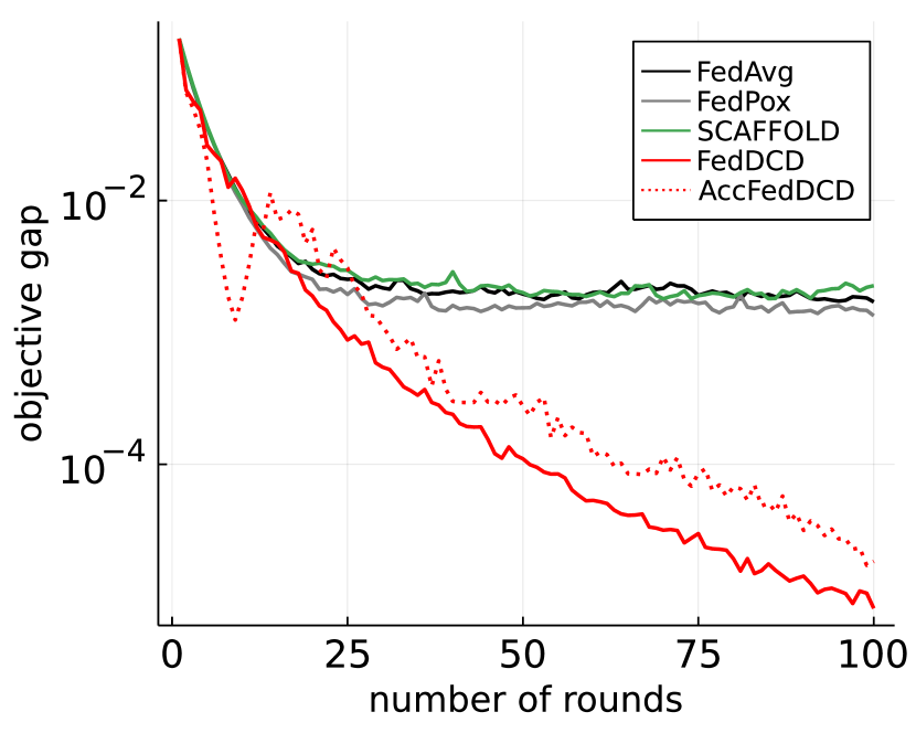
(a) RCV1 with MLR model.

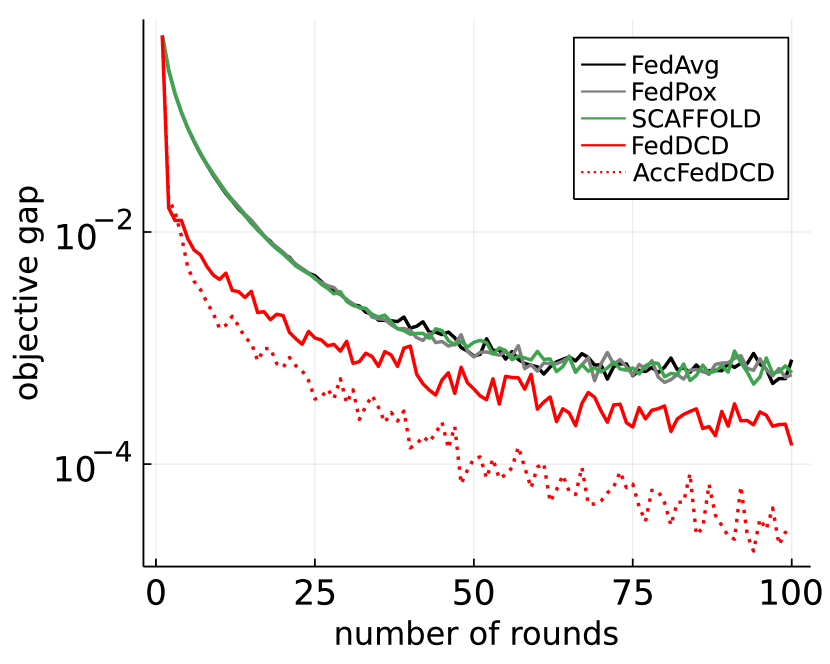
(b) MNIST with MLR model.

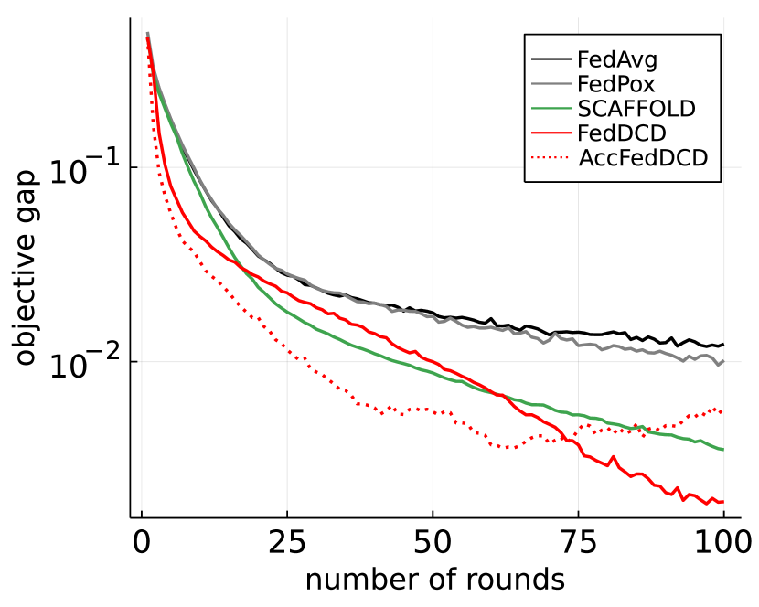
(c) MNIST with MLP model.

Figure 1: Comparison between primal and dual methods; see Section 8.2

8.1 Data sets and implementation

RCV1

The first dataset we use is the Reuters Corpus Volume I (RCV1) dataset [Lewis et al., 2004], where the task is to categorize newswire stories provided by Reuters, Ltd. for research purposes. The number of training points is $20,242$, the number of test points is $677,399$, the number of features is $47,236$ and the number of classes is $2$.

MNIST

The second dataset we use is the well known MNIST dataset [LeCun et al., 1998], where the task is to classify hand-written digits. The number of training points is $60,000$, the number of test points is $10,000$, the number of features is $784$ and the number of classes is $10$.

All datasets are downloaded from the website of LIBSVM [Chang and Lin, 2011].

Model

For RCV1 dataset, we train a multinomial logistic regression (MLR) model. For MNIST dataset, we train two models: a MLR model and a 2-layer multilayer perceptron (MLP) model with 32 neurons in the hidden layer.

Data distribution

For the experiments in Section 8.2 and Section 8.3, we distribute the data to clients in an i.i.d. fashion, i.e., the local datasets are uniformly sampled without replacement and the numbers of local training samples are equal among all the clients. For the experiments in Section 8.4, we distribute the data to clients in a non-i.i.d. fashion, i.e., each client gets samples of only two classes and the numbers of local training samples are not equal, which is the same setting as in the FedAvg paper [McMahan et al., 2017].

Implementation

We set the number of clients to be $100$ for all experiments. We implement the variants of FedDCD algorithm proposed in this paper, as well as the primal methods mentioned above in the Julia language [Bezanson et al., 2017]. Our code is publicly available at https://github.com/ZhenanFanUBC/FedDCD.jl. For the primal methods, we try the number of local epochs to be $5$ or $20$ and report the best result. For dual methods, when the model is MLR, we compute the local gradient via $10$ steps of Newton updates, and when the model is MLP, we compute the local gradient via $20$ steps of ADAM [Kingma and Ba, 2014] updates (we locally perform 5 epochs SGD when the data is non-i.i.d. distributed). All the experiments are conducted on a Linux server with 8 CPUs and 64 GB memory.

8.2 Comparison between primal and dual methods

We compare the performances between the well-known primal methods listed above and the dual method we proposed. We set the number of active clients in each round $\tau=30$ for all methods. The experiment results is shown in Figure 1, As we can see from the plots, FedDCD and AccFedDCD have better convergence in terms of communication for the MLR models compared with primal methods and perform similarly as SCAFFOLD for the MLP model.

8.3 Impact of participation rate

We examine the impact of participation rate for both primal and dual methods. We set the number of active clients in each round $\tau\in\{5,10,30\}$ for all the primal and dual methods. We report the number of communication rounds required by different algorithms to achieve certain objective gap $\epsilon\in\{10^{-3},10^{-2},10^{-1}\}$. The results are summarized in Table 2. We observe that FedDCD and AccFedDCD outperform other primal methods in most settings, the trend is obvious especially when the participation rate is high and the target objective gap is small. The observation is consistent with our analysis in Section 4.

		MLR for MNIST	MLR for RCV1	MLP for MNIST
Setup	Algorithm	# rounds	# rounds	# rounds
$\tau=30,\epsilon=10^{-3}$	FedAvg	51	$>100$	$>100$
	FedProx	47	$>100$	$>100$
	SCAFFOLD	45	$>100$	$>100$
	FedDCD	28	24	$>100$
	AccFedDCD	15	30	$>100$
$\tau=30,\epsilon=10^{-2}$	FedAvg	17	10	$>100$
	FedProx	17	10	99
	SCAFFOLD	17	11	44
	FedDCD	4	10	49
	AccFedDCD	3	5	28
$\tau=10,\epsilon=10^{-2}$	FedAvg	19	11	$>500$
	FedProx	18	11	$>500$
	SCAFFOLD	18	11	$418$
	FedDCD	19	27	96
	AccFedDCD	14	14	$>500$
$\tau=5,\epsilon=10^{-1}$	FedAvg	5	3	88
	FedProx	5	3	83
	SCAFFOLD	5	3	79
	FedDCD	3	5	5
	AccFedDCD	1	1	4

Table 2: Number of rounds required under different setups, $\epsilon$ stands for the target objective gap. We bold the smallest number of rounds for each setup of $\tau$ and $\epsilon$.

8.4 Impact of data heterogeneity

We examine the impact of data heterogeneity for both primal and dual methods. We distribute the data to clients in an non-i.i.d. fashion as described in Section 8.1. We set the number of active clients in each round $\tau=30$ for all the primal and dual methods. The training curves are shown in Figure 2 and the final testing accuracies from different algorithms are reported in Table 3. As we can see from the plots, for the MLR model, AccFedDCD out performs all the other algorithms, and for the MLP model, FedDCD and AccFedDCD have similar performance as SCAFFOLD. Besides, when compared with Figure 1(b) and Figure 1(c), the convergence behaviors of FedDCD and AccFedDCD become worse, which reflects the impact of data heterogeneity. From Table 3, we can observe that both FedDCD, AccFedDCD can reach testing accuracy as good as SCAFFOLD.

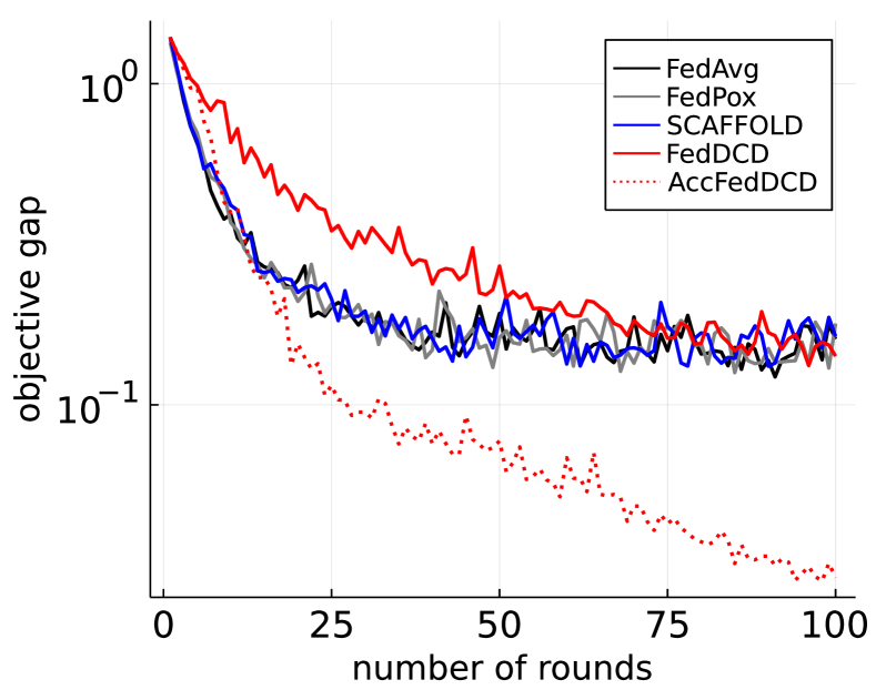
(a) MNIST with MLR model.

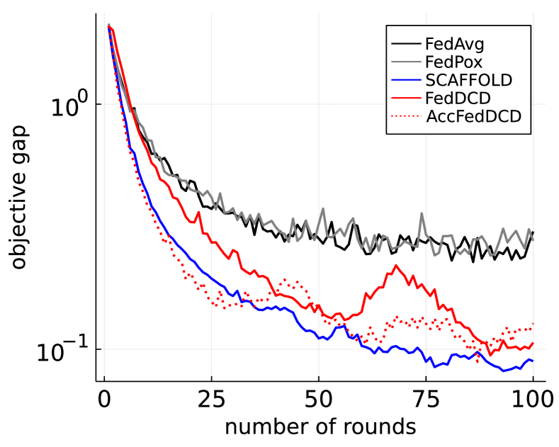
(b) MNIST with MLP model.

Figure 2: Impact of data heterogeneity; see Section 8.4.

	MLR	MLP
FedAvg	88.30%	88.17%
FedProx	88.67%	87.92%
SCAFFOLD	88.47%	90.23%
FedDCD	88.16%	90.02%
AccFedDCD	89.24%	90.32%

Table 3: Test accuracy.

9 Conclusion and future directions

In this paper, by tackling the dual problem of federated optimization, we propose the federated dual coordinate descent (FedDCD) algorithm and its variants based on the random block coordinate descent algorithm [Necoara et al., 2017]. Both FedDCD and its variants satisfy the desired properties for federated learning and have better communication complexities than other SGD-based federated learning algorithms under certain scenarios.

More importantly, FedDCD provides a general framework for federated optimization and suggests many interesting future research directions. First, it is possible to develop an asynchronous version of FedDCD by leveraging well-studied analysis of asynchronous parallel coordinate descent methods [Liu and Wright, 2015; Liu et al., 2015]. Next, one might consider client sampling strategies other than the standard uniform sampling. For example, there are some recent studies of the coordinate descent with the greedy selection rule [Nutini et al., 2015, 2017; Fang et al., 2020], which can be adopted with FedDCD. Finally, the lower bound of complexity of first-order methods with random participation for federated optimization is still an open problem. As we have shown in Section 7, our lower bound analysis has a $\mathcal{O}(\sqrt{N})$ gap to the upper bound of accelerated FedDCD. We hope to explore whether the lower bound can be further tightened or an algorithm with a faster convergence rate can be developed.

Appendix A Structure of the appendix

In this appendix, we include some materials to supplement the main context. To make our argument cleaner, we consider the following optimization problem

$$\displaystyle\mathop{\hbox{minimize}}_{x_{1},\dots,x_{n}\in\mathbb{R}}\enspace h(x)\coloneqq\sum_{i=1}^{n}h_{i}(x_{i})\enspace\mathop{\hbox{subject to}}\enspace\sum_{i=1}^{n}x_{i}=0.$$ (15)

For simplicity, we assume $h_{i}$’s to be 1-dimensional scalar functions and all the results presented in the appendix can be easily extended to the block case. In this appendix, we analyze the convergence behavior of several extensions to the randomized block coordinate descent (RBCD) method proposed by Necoara et al. [2017]. In Appendix B, we present some useful lemmas. We provide a convergence analysis for inexact RBCD and accelerated RBCD respectively in Appendix C and Appendix D. We provide the proofs for all the theorems in the main context in Appendix E. Finally, in Appendix F, we show the complexity lower bound for solving problem (P).

Appendix B Preliminaries and Lemmas

In this section, we introduce some assumptions and notations used in the appendix. Throughout the appendix, we assume $h$ to be coordinate-wise smooth and strongly convex, which is formalized in the following assumption.

Assumption B.1 (Structure of function $h$).

There exists positive constants $\{L_{i}\mid i\in[N]\}$ and $\{\mu_{i}\mid i\in[N]\}$ such that for all $x,y\in\mathbb{R}$ and $i\in[N]$,

$$h_{i}(x) \leq h_{i}(y)+\langle\nabla h_{i}(y),x-y\rangle+\frac{L_{i}}{2}(x-y)^{2}$$ (smoothnes)

$$h_{i}(x) \geq h_{i}(y)+\langle\nabla h_{i}(y),x-y\rangle+\frac{\mu_{i}}{2}(x-y)^{2}.$$ (strong convexity)

Let $L_{\max}\coloneqq\max_{i\in[n]}L_{i},L_{\min}\coloneqq\min_{i\in[n]}L_{i},\mu_{\max}\coloneqq\max_{i\in[n]}\mu_{i},\mu_{\min}\coloneqq\min_{i\in[n]}\mu_{i}$ and $\boldsymbol{L}=\operatorname{diag}(L_{1},L_{2},\ldots,L_{n})$. Sometimes we will simply write $\mu_{\min}$ as $\mu$ in our analysis. We denote the set of coordinates selected as $I\subseteq[n]$. Given a vector $x\in\mathbb{R}^{n}$, we define $x_{I}\coloneqq\sum_{i\in I}x_{i}e_{i}$. The identity matrix is written as $\mathbb{I}$ and $\mathbb{I}_{I}$ is the diagonal matrix with $i$th diagonal element equal to $1$ if $i\in I$ and $0$ otherwise. The constraint sets

$$\mathcal{C}=\left\{x\in\mathbb{R}^{n}~{}\Bigg{|}~{}\sum_{i=1}^{n}x_{i}=0\right\}\quad\text{and}\quad\mathcal{C}_{I}=\left\{x\in\mathbb{R}^{n}~{}\Bigg{|}~{}\sum_{i\in I}x_{i}=0\right\}$$

are used repeatedly in our analysis. Given $1<\tau\leq n$, we use $\mathcal{P}_{\tau}$ to denote all possible subsets of $[n]$ that has cardinality $\tau$, e.g., $\mathcal{P}_{\tau}=\{I\subseteq[n]\mid|I|=\tau\}$. We consider the distribution

$$\mathbb{P}(I)=\frac{e_{I}^{T}\boldsymbol{L}^{-1}e_{I}}{\sum_{J\in\mathcal{P}_{\tau}}e_{J}^{T}\boldsymbol{L}^{-1}e_{J}}$$

when generating random indices set $I\subseteq[n]$. This distribution is identical to the one used in Necoara et al. [2017]. We refer readers to their work for more intuition behind this sampling scheme. Given a PSD matrix $W\in\mathbb{R}^{n\times n}$, we define the norm $\|x\|_{W}^{2}\coloneqq x^{T}Wx~{}\forall x\in\mathbb{R}^{n}$ and we also define $\langle x,y\rangle_{W}$ as $x^{T}Wy$. The projection operator on $\mathcal{C}_{I}$ with respect to $\|\cdot\|_{W}$ is defined as

$$\operatorname{proj}_{\mathcal{C}_{I}}^{W}(x)=\mathop{\hbox{arg\,min}}_{y}\|y-x\|_{W}^{2}\enspace\mathop{\hbox{subject to}}\enspace y\in\mathcal{C}_{I}.$$

We define the following four operators, which are widely used in our analysis:

$$P_{I}\coloneqq\operatorname{proj}_{\mathcal{C}_{I}}^{\boldsymbol{L}}\circ\mathbb{I}_{I},\quad G_{I}\coloneqq P_{I}\circ\boldsymbol{L}^{-1},\quad P_{\tau}\coloneqq\mathbb{E}_{I}[P_{I}],\quad G_{\tau}\coloneqq\mathbb{E}_{I}[G_{I}].$$

Next we present some useful lemmas for our analysis.

Lemma B.2 (Expression of the projection operator).

The projection operator on the set $C_{I}$ can be expressed as

$$\operatorname{proj}_{\mathcal{C}_{I}}^{W}(x)=\left(I-\frac{1}{e_{I}^{T}W^{-1}e_{I}}W^{-1}e_{I}e_{I}^{T}\right)x.$$

Proof.

By definition, the projection operator can be expressed as

$$\operatorname{proj}_{\mathcal{C}_{I}}^{W}(x)=\mathop{\hbox{arg\,min}}_{d}\frac{1}{2}(d-x)^{T}W(d-x)\enspace\mathop{\hbox{subject to}}\enspace e_{I}^{T}d=0.$$ (16)

The Lagrangian function with respect to eq. 16 takes the form

$$\mathcal{L}(d,\lambda)=\frac{1}{2}(d-x)^{T}W(d-x)+\lambda e_{I}^{T}d.$$

By checking the optimility condition with respect to $d$, we have

$$\nabla_{d}\mathcal{L}(d,\lambda)=W(d-x)+\lambda e_{I}=0\enspace\Rightarrow\enspace d=x-\lambda W^{-1}e_{I}.$$

By checking the optimility condition with respect to $\lambda$, we have

$$\nabla_{\lambda}\mathcal{L}(d,\lambda)=e_{I}^{T}d=e_{I}^{T}x-\lambda e_{I}^{T}W^{-1}e_{I}=0\enspace\Rightarrow\enspace\lambda=\frac{e_{I}^{T}x}{e_{I}^{T}W^{-1}e_{I}}.$$

We can thus conclude that

$$\operatorname{proj}_{\mathcal{C}_{I}}^{W}(x)=\left(I-\frac{1}{e_{I}^{T}W^{-1}e_{I}}W^{-1}e_{I}e_{I}^{T}\right)x.$$

∎

As a consequence of Lemma B.2, we have the following expressions for $P_{I}$ and $G_{I}$:

$$P_{I} =\mathbb{I}_{I}-\frac{1}{e_{I}^{T}\boldsymbol{L}^{-1}e_{I}}\boldsymbol{L}^{-1}e_{I}e_{I}^{T}$$

$$G_{I} =\mathbb{I}_{I}\boldsymbol{L}^{-1}-\frac{1}{e_{I}^{T}\boldsymbol{L}^{-1}e_{I}}\boldsymbol{L}^{-1}e_{I}e_{I}^{T}\boldsymbol{L}^{-1}.$$

Our next lemma gives explicit expressions for the expectations of $P_{I}$ and $G_{I}$.

Lemma B.3 (Statistical properties of matrices $P$ and $G$).

For any $I\subseteq[n]$, we have the following relationships:

$$G_{I} =G_{I}^{T},$$ (Symmetric)

$$P_{I} =P_{I}^{2},$$ (Idempotent)

$$G_{I} =G_{I}^{T}\boldsymbol{L}G_{I},$$ (17)

$$P_{\tau}\coloneqq\mathbb{E}_{I}[P_{I}] =\frac{\tau-1}{n-1}P_{[n]},$$ (18)

$$G_{\tau}\coloneqq\mathbb{E}_{I}[G_{I}] =\frac{\tau-1}{n-1}G_{[n]},$$ (19)

$$\mathbb{E}_{I}\left[\|G_{I}x\|^{2}_{\boldsymbol{L}}\right] =\frac{\tau-1}{n-1}\|G_{[n]}x\|^{2}_{\boldsymbol{L}}\qquad\forall x\in\mathbb{R}^{n},$$ (20)

$$\mathbb{E}_{I}\left[\langle G_{I}x,y\rangle_{\boldsymbol{L}}\right] =\frac{\tau-1}{n-1}\langle x,y\rangle\qquad\forall x,y\in\mathcal{C}.$$ (21)

Proof.

The symmetry of $G_{I}$ and the idempotent of $P_{I}$ follow directly from the definitions.

For eq. 17, we have

$$G_{I}^{T}\boldsymbol{L}G_{I} ~{}=~{}G_{I}\boldsymbol{L}G_{I}~{}=~{}P_{I}\boldsymbol{L}^{-1}\boldsymbol{L}P_{I}\boldsymbol{L}^{-1}~{}=~{}P_{I}\boldsymbol{L}^{-1}~{}=~{}G_{I}.$$

The expression of $G_{\tau}$ follows directly from [Necoara et al., 2017, Theorem 3.3]. So we only need to derive the expression fro $P_{\tau}$. By definition, we have

$$P_{\tau} =\mathbb{E}_{I}[P_{I}]$$

$$=\sum_{I\in\mathcal{P}_{\tau}}\mathbb{P}(I)\left[\mathbb{I}_{I}-\frac{1}{e_{I}^{T}W^{-1}e_{I}}W^{-1}e_{I}e_{I}^{T}\right]$$

$$=\sum_{I\in\mathcal{P}_{\tau}}\frac{e_{I}^{T}W^{-1}e_{I}}{\sum_{J\in\mathcal{P}_{\tau}}e_{J}^{T}W^{-1}e_{J}}\left[\mathbb{I}_{I}-\frac{1}{e_{I}^{T}W^{-1}e_{I}}W^{-1}e_{I}e_{I}^{T}\right]$$

$$=\underbrace{\sum_{I\in\mathcal{P}_{\tau}}\frac{e_{I}^{T}W^{-1}e_{I}}{\sum_{J\in\mathcal{P}_{\tau}}e_{J}^{T}W^{-1}e_{J}}\mathbb{I}_{I}}_{(a)}-\underbrace{\sum_{I\in\mathcal{P}_{\tau}}\frac{1}{\sum_{J\in\mathcal{P}_{\tau}}e_{J}^{T}W^{-1}e_{J}}W^{-1}e_{I}e_{I}^{T}}_{(b)}.$$

Let $\Sigma_{\tau}=\sum_{J\in\mathcal{P}_{\tau}}e_{J}^{T}W^{-1}e_{J}$. Then the first component can be expressed as

$$(a) =\Sigma_{\tau}^{-1}\sum_{I\in\mathcal{P}_{\tau}}e_{I}^{T}W^{-1}e_{I}\mathbb{I}_{I}$$

$$=\Sigma_{\tau}^{-1}\sum_{j=1}^{\binom{n}{\tau}}\left(\sum_{u\in I_{j}}w_{u}^{-1}\right)\left(\sum_{v\in I_{j}}e_{v}e_{v}^{T}\right)$$

$$=\Sigma_{\tau}^{-1}\sum_{j=1}^{\binom{n}{\tau}}\sum_{u\in I_{j}}\sum_{v\in I_{j}}w_{u}^{-1}e_{v}e_{v}^{T}$$

$$=\Sigma_{\tau}^{-1}\sum_{u=1}^{n}\sum_{v=1}^{n}w_{u}^{-1}e_{v}e_{v}^{T}\left(\sum_{j=1}^{\binom{n}{\tau}}\mathbbm{1}_{u,v\in I_{j}}\right)$$

$$=\binom{n-2}{\tau-2}\Sigma_{\tau}^{-1}e^{T}W^{-1}e\mathbb{I},$$

and the second component can be expressed as

$$(b) =\Sigma_{\tau}^{-1}\sum_{I\in\mathcal{P}_{\tau}}W^{-1}e_{I}e_{I}^{T}$$

$$=\Sigma_{\tau}^{-1}W^{-1}\sum_{j=1}^{\binom{n}{\tau}}\sum_{u\in I_{j}}\sum_{v\in I_{j}}e_{u}e_{v}^{T}$$

$$=\Sigma_{\tau}^{-1}W^{-1}\sum_{u=1}^{n}\sum_{v=1}^{n}e_{u}e_{v}^{T}\left(\sum_{j=1}^{\binom{n}{\tau}}\mathbbm{1}_{u,v\in I_{j}}\right)$$

$$=\binom{n-2}{\tau-2}\Sigma_{\tau}^{-1}W^{-1}ee^{T}.$$

Therefore, we have

$$P_{\tau}=\binom{n-2}{\tau-2}\Sigma_{\tau}^{-1}e^{T}W^{-1}eP_{[n]}.$$

Next, we show that $\binom{n-2}{\tau-2}\Sigma_{\tau}^{-1}e^{T}W^{-1}e=\frac{\tau-1}{n-1}$. Indeed, we have

$$\binom{n-2}{\tau-2}\Sigma_{\tau}^{-1}e^{T}W^{-1}e =\binom{n-2}{\tau-2}\frac{1}{\sum_{J\in\mathcal{P}_{\tau}}e_{J}^{T}W^{-1}e_{J}}e^{T}W^{-1}e$$

$$=\binom{n-2}{\tau-2}\frac{1}{\binom{n-1}{\tau-1}e^{T}W^{-1}e}e^{T}W^{-1}e$$

$$=\frac{\tau-1}{n-1}.$$

This finishes the proof for eq. 18.

For any $x\in\mathbb{R}^{n}$,

$$\mathbb{E}_{I}\left[\|G_{I}x\|_{\boldsymbol{L}}^{2}\right] ~{}=~{}\mathbb{E}_{I}\left[x^{T}G_{I}^{T}\boldsymbol{L}G_{I}x\right]$$

$$~{}=~{}\mathbb{E}_{I}\left[x^{T}G_{I}x\right]\qquad\text{(By \lx@cref{creftype~refnum}{eq:GeqGTLG})}$$

$$~{}=~{}\frac{\tau-1}{n-1}x^{T}G_{[n]}x\qquad\text{(By \lx@cref{creftype~refnum}{eq:Gnexp})}$$

$$~{}=~{}\frac{\tau-1}{n-1}\|G_{[n]}x\|^{2}_{\boldsymbol{L}}.$$

This finishes the proof for eq. 20.

Finally, we prove eq. 21,

$$\mathbb{E}\left[\langle G_{I}x,y\rangle_{\boldsymbol{L}}\right] =\frac{\tau-1}{n-1}\langle G_{[n]}x,y\rangle_{\boldsymbol{L}}$$

$$=\frac{\tau-1}{n-1}\langle x,G_{[n]}\boldsymbol{L}y\rangle$$

$$=\frac{\tau-1}{n-1}\langle x,P_{[n]}\boldsymbol{L}^{-1}\boldsymbol{L}y\rangle$$

$$=\frac{\tau-1}{n-1}\langle x,y\rangle\qquad\text{(Since $y\in\mathcal{C}$)}.$$

∎

Lemma B.4 (Eigenvalues of $G_{[n]}$).

$$\lambda_{1}(G_{[n]}) \leq 1/L_{\min},$$ (22)

$$\lambda_{n}(G_{[n]}) =0.$$ (23)

Proof.

Follows directly from the definition of $G_{[n]}$. ∎

Lemma B.5 (Gradient at optimal).

Let $x^{*}$ be the optimal solution to eq. 15. Then we have $P_{[n]}^{T}\nabla h(x^{*})=0$.

Proof.

Since $x^{*}$ is the optimal solution to eq. 15, by the first order optimality condition, we know that $-\nabla h(x^{*})\in\mathcal{N}_{\mathcal{C}}(x^{*})$, where $\mathcal{N}_{\mathcal{C}}(x^{*})$ is the normal cone of $\mathcal{C}$ at $x^{*}$. By the definition of normal cone, we know that

$$~{}\langle-\nabla h(x^{*}),z-x^{*}\rangle\leq 0\enspace\forall z\in\mathcal{C}$$

$$\Rightarrow~{} ~{}\langle-\nabla h(x^{*}),P_{[n]}z-x^{*}\rangle\leq 0\enspace\forall z\in\mathbb{R}^{n}$$

$$\Rightarrow~{} ~{}\langle-\nabla h(x^{*}),P_{[n]}(z-x^{*})\rangle\leq 0\enspace\forall z\in\mathbb{R}^{n}$$

$$\Rightarrow~{} ~{}\langle-P_{[n]}^{T}\nabla h(x^{*}),z-x^{*}\rangle\leq 0\enspace\forall z\in\mathbb{R}^{n}$$

$$\Rightarrow~{} ~{}\langle-P_{[n]}^{T}\nabla h(x^{*}),z\rangle\leq 0\enspace\forall z\in\mathbb{R}^{n}$$

$$\Rightarrow~{} ~{}P_{[n]}^{T}\nabla h(x^{*})=0.$$

∎

Lemma B.6 (Bound on gradient).

Under Assumption B.1, we have

$$\frac{2\mu}{L_{\max}^{2}}(h(x^{t})-h(x^{*}))\leq\|G_{[n]}\nabla h(x^{t})\|^{2}\leq\frac{2L_{\max}}{L_{\min}^{2}}(h(x^{t})-h(x^{*})),$$

and

$$\frac{2\mu}{L_{\max}}(h(x^{t})-h(x^{*}))\leq\|G_{[n]}\nabla h(x^{t})\|_{\boldsymbol{L}}^{2}\leq\frac{2L_{\max}}{L_{\min}}(h(x^{t})-h(x^{*}))$$

for any $x^{t}\in\mathcal{C}$.

Proof.

We define a helper function $\phi:\mathbb{R}^{n}\to\mathbb{R}$ as

$$\phi(x)\coloneqq h(P_{[n]}x).$$

By the assumption that $h$ is $\mu$-strongly convex, it follows that

$$~{}h(y)\geq h(x)+\langle\nabla h(x),y-x\rangle+\frac{\mu}{2}\|x-y\|^{2}\enspace\forall x,y$$

$$\Rightarrow ~{}h(P_{[n]}y)\geq h(P_{[n]}x)+\langle\nabla h(P_{[n]}x),P_{[n]}y-P_{[n]}x\rangle+\frac{\mu}{2}\|P_{[n]}x-P_{[n]}y\|^{2}\enspace\forall x,y$$

$$\Rightarrow ~{}h(P_{[n]}y)\geq h(P_{[n]}x)+\langle P_{[n]}^{T}\nabla h(P_{[n]}x),y-x\rangle+\frac{\mu}{2}\|P_{[n]}x-P_{[n]}y\|^{2}\enspace\forall x,y$$

$$\Rightarrow ~{}\phi(y)\geq\phi(x)+\langle\nabla\phi(x),y-x\rangle+\frac{\mu}{2}\|P_{[n]}x-P_{[n]}y\|^{2}\enspace\forall x,y$$

$$\Rightarrow ~{}\phi(y)\geq\phi(x)+\langle\nabla\phi(x),y-x\rangle+\frac{\mu}{2}\|x-y\|^{2}\enspace\forall x,y\in\mathcal{C}.$$

Fix $x=x^{t}$ and take minimization with respect to $y\in\mathcal{C}$ to both sides of the inequality, we can get

$$\frac{1}{2}\|\nabla\phi(x^{t})\|^{2}\geq\mu(\phi(x^{t})-\phi(x^{*})).$$

It follows that

$$\|G_{[n]}\nabla h(x^{t})\|^{2} =\|\boldsymbol{L}^{-1}\nabla\phi(x^{t})\|^{2}$$

$$\geq\frac{1}{L_{\max}^{2}}\|\nabla\phi(x^{t})\|^{2}$$

$$\geq\frac{2\mu}{L_{\max}^{2}}(\phi(x^{t})-\phi(x^{*}))$$

$$=\frac{2\mu}{L_{\max}^{2}}(h(x^{t})-h(x^{*})).$$

Similarly, for the $L$-norm, we have

$$\|G_{[n]}\nabla h(x^{t})\|_{\boldsymbol{L}}^{2} =\|\boldsymbol{L}^{-1}\nabla\phi(x^{t})\|_{\boldsymbol{L}}^{2}$$

$$=\|\boldsymbol{L}^{-\frac{1}{2}}\nabla\phi(x^{t})\|^{2}$$

$$\geq\frac{1}{L_{\max}}\|\nabla\phi(x^{t})\|^{2}$$

$$\geq\frac{2\mu}{L_{\max}}(\phi(x^{t})-\phi(x^{*}))$$

$$=\frac{2\mu}{L_{\max}}(h(x^{t})-h(x^{*})).$$

By the same reason and the assumption that $h$ is $L$-smooth, we can conclude that for any $x^{t}$,

$$\phi(x^{t})-\phi(x^{*})\geq\frac{1}{2L_{\max}}\|\nabla\phi(x^{t})\|^{2}.$$

It follows that

$$\|G_{[n]}\nabla h(x^{t})\|^{2} =\|\boldsymbol{L}^{-1}\nabla\phi(x^{t})\|^{2}$$

$$\leq\frac{1}{L_{\min}^{2}}\|\nabla\phi(x^{t})\|^{2}$$

$$\leq\frac{2L_{\max}}{L_{\min}^{2}}(\phi(x^{t})-\phi(x^{*}))$$

$$=\frac{2L_{\max}}{L_{\min}^{2}}(h(x^{t})-h(x^{*})).$$

Similarly, for the $L$-norm, we have

$$\|G_{[n]}\nabla h(x^{t})\|_{\boldsymbol{L}}^{2} =\|L^{-1}\nabla\phi(x^{t})\|_{\boldsymbol{L}}^{2}$$

$$=\|\boldsymbol{L}^{-\frac{1}{2}}\nabla\phi(x^{t})\|^{2}$$

$$\leq\frac{1}{L_{\min}}\|\nabla\phi(x^{t})\|^{2}$$

$$\leq\frac{2L_{\max}}{L_{\min}}(\phi(x^{t})-\phi(x^{*}))$$

$$=\frac{2L_{\max}}{L_{\min}}(h(x^{t})-h(x^{*})).$$

∎

Lemma B.7 (Three-point property with constraint [Tseng, 2008]).

Let $u$ be a convex function, and let $D_{\Phi}(\cdot,\cdot)$ be the Bregman divergence induced by the mirror map $\Phi$. Given a convex constraint set $C\in\mathbb{R}^{d}$. For a given vector $z$, let

$$z^{+}\coloneqq\underset{x\in C}{\arg\min}\{u(x)+D_{\Phi}(x,z)\}.$$ (24)

Then

$$u(x)+D_{\Phi}(x,z)\geq u(z^{+})+D_{\Phi}(z^{+},z)+D_{\Phi}(x,z^{+})\quad\forall x\in C.$$ (25)

Lemma B.8 (Descent lemma).

Under Assumption B.1. Given $x\in\mathbb{R}^{n}$, let $y\coloneqq x-G_{I}\nabla h(x)$, then

$$\mathbb{E}[h(y)]~{}\leq~{}h(x)-\frac{1}{2}\frac{\tau-1}{n-1}\|G_{[n]}\nabla h(x)\|_{\boldsymbol{L}}^{2},$$

and

$$\mathbb{E}[h(y)]-h(x^{*})\leq\left(1-\frac{\mu_{\min}}{L_{\max}}\right)\mathbb{E}[h(x)]-h(x^{*}).$$

Proof.

For the first inequality,

$$\mathbb{E}[h(y)] ~{}\leq~{}\mathbb{E}\left[h(x)+\langle\nabla h(x),y-x\rangle+\frac{1}{2}\|y-x\|_{\boldsymbol{L}}^{2}\right]$$

$$~{}=~{}h(x)-\mathbb{E}\left[\langle\nabla h(x),G_{I}\nabla h(x)\rangle+\frac{1}{2}\|G_{I}\nabla h(x)\|_{\boldsymbol{L}}^{2}\right]$$

$$~{}=~{}h(x)-\frac{1}{2}\frac{\tau-1}{n-1}\|G_{[n]}\nabla h(x)\|_{\boldsymbol{L}}^{2}\quad\text{(By \lx@cref{creftype~refnum}{eq:GnormExp} and \lx@cref{creftype~refnum}{eq:GeqGTLG})}.$$

For the second inequality, apply Lemma B.6 to the above equation, we get

$$\mathbb{E}[h(y)] ~{}\leq~{}h(x)-\frac{\tau-1}{n-1}\frac{\mu_{\min}}{L_{\max}}(h(x)-h(x^{*}))$$

$$\Rightarrow~{}~{}\mathbb{E}[h(y)]-h(x^{*}) ~{}\leq\left(1-\frac{\tau-1}{n-1}\frac{\mu_{\min}}{L_{\max}}\right)(h(x)-h(x^{*})).$$

∎

Appendix C Inexact randomized block coordinate descent

Input: number of participating coordinates in each round $1<\tau\leq n$, $\delta\in(0,1)$

$x_{i}^{(0)}\leftarrow 0$ for all $i\in[n]$, let $r=\frac{\tau-1}{n-1}$.

  [initialization]

1 for $t\leftarrow 0,1,\ldots,T$ do

       $I\leftarrow\mbox{ random set of }\tau\mbox{ coordinates }$

        [randomly select a subset of coordinates]

       $\widetilde{\nabla}h(x^{(t)})\leftarrow 0$

        []

2       for $i\in I$ do

3             $\widetilde{\nabla}_{i}h(x^{(t)})\leftarrow\texttt{oracle}(\widetilde{\nabla}h_{i}(x^{(t-1)}),\delta/2)$

      $x^{(t+1)}\coloneqq x^{(t)}-\eta_{t}G_{I_{t}}\widetilde{\nabla}h(x^{(t)})$

        [update iterate]

4      

return $x^{(T)}$

Algorithm 3 Inexact Random Block Coordinate Descent Method with Linear Constraint

In this section, we analyze the convergence behaviour of RBCD with inexact gradient oracle for solving eq. 15. The detailed algorithm is shown in Algorithm 3 and the convergence rate is shown in the following theorem.

Theorem C.1.

Assume Assumption B.1 is satisfied. Let

$$\kappa ~{}=~{}\frac{r\mu}{8L_{\max}}\min\left\{\frac{1}{4},\frac{L_{\min}^{\frac{3}{2}}}{4r^{\frac{1}{2}}L_{\max}^{\frac{3}{2}}}\right\}~{}\in(0,1)$$

$$\delta ~{}=~{}(1-\kappa)/2,$$

$$\eta ~{}=~{}\min\left\{\frac{1}{4},\frac{L_{\min}^{\frac{3}{2}}}{4r^{\frac{1}{2}}L_{\max}^{\frac{3}{2}}}\right\}$$ (26)

Let $x^{(T)}$ be the iterate generated from Algorithm 3, then we have

$$\mathbb{E}\left[h(x^{(T)})\right]-h(x^{*})\leq(1-\kappa)^{T}\left[h(x^{(0)})-h(x^{*})\right].$$

Our analysis is enlightened by a recent work from Liu et al. [2021], who extended the distributed dual accelerated gradient algorithm [Scaman et al., 2017] with lazy dual gradient. Before presenting the proof of Theorem C.1, we first cite an important lemma from [Liu et al., 2021] which gives a bound on the difference between inexact and exact gradients.

Lemma C.2 (Liu et al. [2021, Lemma 1]).

Given $\delta>0$. Let $\{x^{(t)}\}_{t=0}^{\infty}$ and $\{\widetilde{\nabla}h(x^{(t)})\}_{t=0}^{\infty}$ be generated from Algorithm 3 with $\delta/2$-inexact gradient oracle. Then $\forall t\in\mathbb{N}$,

$$\mathbb{E}\left[\|\widetilde{\nabla}h(x^{(t)})-{\nabla}h(x^{(t)})\|^{2}\right]\leq\sum_{j=0}^{t-1}\delta^{t-j}\mathbb{E}\left[\|\nabla h(x^{(j)})-{\nabla}h(x^{(j+1)})\|^{2}\right].$$ (27)

Proof.

An alternative proof can be found in Liu et al. [2021, Appendix A]. Here we reproduce it for completeness. By the definition of $\delta$-inexact gradient oracle and the warm start point, we have

$$\mathbb{E}\left[\|\widetilde{\nabla}h(x^{(t)})-{\nabla}h(x^{(t)})\|^{2}~{}\Big{|}~{}x^{(t)}\right] \leq\frac{\delta}{2}\|\widetilde{\nabla}h(x^{(t-1)})-{\nabla}h(x^{(t)})\|^{2}$$

$$\leq\delta\|\widetilde{\nabla}h(x^{(t-1)})-{\nabla}h(x^{(t-1)})\|^{2}+\delta\|{\nabla}h(x^{(t-1)})-{\nabla}h(x^{(t)})\|^{2}.$$

Take expectation on both sides of the above inequality and apply it recursively, we obtain the desired result. ∎

Next, we show the proof for Theorem C.1.

Proof.

First, we construct a Lyapunov function

$$L_{t}\coloneqq\mathbb{E}[h(x^{(t)})-h(x^{*})+A_{t}],$$

where

$$A_{t}\coloneqq M\sum_{j=0}^{t-1}\left(\frac{1-\kappa}{2}\right)^{t-1-j}\|\nabla h(x^{(j)})-{\nabla}h(x^{(j+1)})\|^{2}\quad\forall t\geq 1,\quad A_{0}=0$$

for some $M>0$ and $\kappa\in(0,1)$ which we will define later.

Next, we show that a careful choice of hyperparameters can lead to a linear convergence rate of the Lyapunov function. We begin with the smoothness property of $h$,

$$\mathbb{E}\left[h(x^{(t+1)})~{}\Big{|}~{}x^{(t)}\right]$$

$$\leq~{} h(x^{(t)})-\langle\nabla h(x^{(t)}),r\eta G_{[n]}\widetilde{\nabla}h(x^{(t)})\rangle+\frac{r\eta^{2}}{2}\|G_{[n]}\widetilde{\nabla}h(x^{(t)})\|_{\boldsymbol{L}}^{2}$$

$$\leq~{} h(x^{(t)})-r\eta\|G_{[n]}\nabla h(x^{(t)})\|_{\boldsymbol{L}}^{2}-\vphantom{\frac{r\eta^{2}L_{\max}}{2}}r\eta\langle\nabla h(x^{(t)}),G_{[n]}(\widetilde{\nabla}h(x^{(t)})-\nabla h(x^{(t)}))\rangle+\frac{r\eta^{2}}{2}\|G_{[n]}\widetilde{\nabla}h(x^{(t)})\|_{\boldsymbol{L}}^{2}$$

$$\leq~{} h(x^{(t)})-r\eta\|G_{[n]}\nabla h(x^{(t)})\|_{\boldsymbol{L}}^{2}+r\eta\left(\frac{1}{2}\|\boldsymbol{L}^{\frac{1}{2}}G_{[n]}\nabla h(x^{(t)})\|_{2}^{2}+\frac{1}{2}\|\boldsymbol{L}^{\frac{1}{2}}G_{[n]}(\widetilde{\nabla}h(x^{(t)})-\nabla h(x^{(t)}))\|_{2}^{2}\right)$$

$$+\frac{r\eta^{2}}{2}\|G_{[n]}(\widetilde{\nabla}h(x^{(t)})-\nabla h(x^{(t)})+\nabla h(x^{(t)}))\|_{\boldsymbol{L}}^{2}$$

$$\leq~{} h(x^{(t)})-r\eta\|G_{[n]}\nabla h(x^{(t)})\|_{\boldsymbol{L}}^{2}+r\eta\left(\frac{1}{2}\|G_{[n]}\nabla h(x^{(t)})\|_{\boldsymbol{L}}^{2}+\frac{1}{2}\|G_{[n]}(\widetilde{\nabla}h(x^{(t)})-\nabla h(x^{(t)}))\|_{\boldsymbol{L}}^{2}\right)$$

$$+r\eta^{2}\|G_{[n]}(\widetilde{\nabla}h(x^{(t)})-\nabla h(x^{(t)}))\|_{\boldsymbol{L}}^{2}+r\eta^{2}\|G_{[n]}\nabla h(x^{(t)})\|_{\boldsymbol{L}}^{2}.$$ (28)

By taking the expectation of both sides with respect to $x^{(t)}$, we get

$$\mathbb{E}\left[h(x^{(t+1)})\right]~{}\leq~{} \mathbb{E}\left[h(x^{(t)})-\left(\frac{r\eta}{2}-r\eta^{2}\right)\|G_{[n]}\nabla h(x^{(t)})\|_{\boldsymbol{L}}^{2}+\left(\frac{r\eta}{2}+r\eta^{2}\right)\|G_{[n]}(\widetilde{\nabla}h(x^{(t)})-\nabla h(x^{(t)})\|_{\boldsymbol{L}}^{2}\right]$$

$$~{}\leq~{} \mathbb{E}\bigg{[}h(x^{(t)})-\left(\frac{r\eta}{2}-r\eta^{2}\right)\|G_{[n]}\nabla h(x^{(t)})\|_{\boldsymbol{L}}^{2}$$

$$+\left(\frac{r\eta}{2}+r\eta^{2}\right)\frac{L_{\max}}{L_{\min}^{2}}\sum_{j=0}^{t-1}\delta^{t-j}\|\nabla h(x^{(j)})-{\nabla}h(x^{(j+1)})\|^{2}\bigg{]},$$ (29)

where the last inequality follows from Lemma B.4 and Lemma C.2. In order to establish the linear convergence of the Lyapunov function, we add and substract the term $\alpha\mathbb{E}[\|\nabla h(x^{(t)})-{\nabla}h(x^{(t+1)})\|^{2}]$ to the RHS of eq. 29, where $\alpha>0$ is some positive scalar. Then eq. 29 becomes

$$\mathbb{E}\left[h(x^{(t+1)})\right]\leq~{} \mathbb{E}\bigg{[}h(x^{(t)})-\left(\frac{r\eta}{2}-r\eta^{2}\right)\|G_{[n]}\nabla h(x^{(t)})\|_{\boldsymbol{L}}^{2}+\alpha\|\nabla h(x^{(t)})-{\nabla}h(x^{(t+1)})\|^{2}$$

$$+\left(\frac{r\eta}{2}+r\eta^{2}\right)\frac{L_{\max}}{L_{\min}^{2}}\sum_{j=0}^{t-1}\delta^{t-j}\|\nabla h(x^{(j)})-{\nabla}h(x^{(j+1)})\|^{2}-\alpha\|\nabla h(x^{(t)})-{\nabla}h(x^{(t+1)})\|^{2}\bigg{]}.$$ (30)

We also know that

$$\mathbb{E}\left[\alpha\|\nabla h(x^{(t)})-{\nabla}h(x^{(t+1)})\|^{2}\right]$$

$$~{}\leq~{} \mathbb{E}\left[\frac{\alpha}{L_{\min}}\|\nabla h(x^{(t)})-{\nabla}h(x^{(t+1)})\|_{\boldsymbol{L}}^{2}\right]$$

$$~{}\leq~{} \mathbb{E}\left[\frac{\alpha L_{\max}^{2}}{L_{\min}}\|\eta G_{I_{t}}\widetilde{\nabla}h(x^{(t)})\|_{\boldsymbol{L}}^{2}\right]\qquad\text{(By $L_{\max}$-smoothness of $h$)}$$

$$~{}\leq~{} \frac{\alpha rL_{\max}^{2}\eta^{2}}{L_{\min}}\mathbb{E}\left[\|G_{[n]}\widetilde{\nabla}h(x^{(t)})\|_{\boldsymbol{L}}^{2}\right]\qquad\text{(By \lx@cref{creftype~refnum}{eq:GnormExp})}$$

$$~{}\leq~{} \frac{2\alpha rL_{\max}^{2}\eta^{2}}{L_{\min}}\mathbb{E}\left[\|G_{[n]}\nabla h(x^{(t)})\|^{2}_{\boldsymbol{L}}\right]+\frac{2\alpha rL_{\max}^{2}\eta^{2}}{L_{\min}}\mathbb{E}\left[\|G_{[n]}(\widetilde{\nabla}h(x^{(t)})-\nabla h(x^{(t)}))\|^{2}_{\boldsymbol{L}}\right]$$

$$~{}\leq~{} \frac{2\alpha rL_{\max}^{2}\eta^{2}}{L_{\min}}\mathbb{E}\left[\|G_{[n]}\nabla h(x^{(t)})\|^{2}_{\boldsymbol{L}}\right]+\frac{2\alpha r\eta^{2}L_{\max}^{3}}{L_{\min}^{3}}\mathbb{E}\left[\|\widetilde{\nabla}h(x^{(t)})-\nabla h(x^{(t)})\|^{2}\right]$$

$$~{}\leq~{} \frac{2\alpha rL_{\max}^{2}\eta^{2}}{L_{\min}}\mathbb{E}\left[\|G_{[n]}\nabla h(x^{(t)})\|^{2}_{\boldsymbol{L}}\right]+\frac{2\alpha r\eta^{2}L_{\max}^{3}}{L_{\min}^{3}}\mathbb{E}\left[\sum_{j=0}^{t-1}\delta^{t-j}\|\nabla h(x^{(j)})-{\nabla}h(x^{(j+1)})\|^{2}\right],$$

the last inequality is from Lemma C.2. Now we can determine the hyperparameters in the Lyapunov function by plugging the above inequality into eq. 30

$$\mathbb{E}\left[h(x^{(t+1)})\right]$$

$$~{}\leq~{} \mathbb{E}\Bigg{[}h(x^{(t)})-{\left(\frac{r\eta}{2}-r\eta^{2}-\frac{2\alpha rL_{\max}^{2}\eta^{2}}{L_{\min}}\right)}\|G_{[n]}\nabla h(x^{(t)})\|_{\boldsymbol{L}}^{2}$$

$$+{\left(\frac{r\eta}{2}+r\eta^{2}+\frac{2\alpha r\eta^{2}L_{\max}^{2}}{L_{\min}}\right)\frac{L_{\max}}{L_{\min}^{2}}\sum_{j=0}^{t-1}\delta^{t-j}\|\nabla h(x^{(j)})-{\nabla}h(x^{(j+1)})\|^{2}-\alpha\|\nabla h(x^{(t)})-{\nabla}h(x^{(t+1)})\|^{2}}\Bigg{]}$$

$$~{}\leq~{} \mathbb{E}\Bigg{[}h(x^{(t)})-\underbrace{\left(\frac{r\eta}{2}-r\eta^{2}-\frac{2\alpha rL_{\max}^{2}\eta^{2}}{L_{\min}}\right)\frac{2\mu}{L_{\max}}}_{\kappa}(h(x^{(t)})-h(x^{*}))\qquad\text{(By~{}\lx@cref{creftypecap~refnum}{lemma:GnormLowerAndUpperBound})}$$

$$+\underbrace{\left(\frac{r\eta}{2}+r\eta^{2}+\frac{2\alpha r\eta^{2}L_{\max}^{2}}{L_{\min}}\right)\frac{L_{\max}}{L_{\min}^{2}}\sum_{j=0}^{t-1}\delta^{t-j}\|\nabla h(x^{(j)})-{\nabla}h(x^{(j+1)})\|^{2}-\alpha\|\nabla h(x^{(t)})-{\nabla}h(x^{(t+1)})\|^{2}}_{\overset{\rm{(i)}}{\leq}(1-\kappa)A_{t}-A_{t+1}}\Bigg{]},$$ (31)

where we let $M\coloneqq\left(\frac{r\eta}{2}+r\eta^{2}+\frac{2\alpha r\eta^{2}L_{\max}^{2}}{L_{\min}}\right)\frac{L_{\max}}{L_{\min}^{2}}$ and $\alpha\geq M$, (i) comes from the following derivation

$$\left(\frac{r\eta}{2}+r\eta^{2}+\frac{2\alpha r\eta^{2}L_{\max}^{2}}{L_{\min}}\right)\frac{L_{\max}}{L_{\min}^{2}}\sum_{j=0}^{t-1}\delta^{t-j}\|\nabla h(x^{(j)})-{\nabla}h(x^{(j+1)})\|^{2}-\alpha\|\nabla h(x^{(t)})-{\nabla}h(x^{(t+1)})\|^{2}$$

$$\leq~{} M\sum_{j=0}^{t-1}\delta^{t-j}\|\nabla h(x^{(j)})-{\nabla}h(x^{(j+1)})\|^{2}-M\|\nabla h(x^{(t)})-{\nabla}h(x^{(t+1)})\|^{2}$$

$$=~{} M\sum_{j=0}^{t-1}\left(\frac{1-\kappa}{2}\right)^{t-j}\|\nabla h(x^{(j)})-{\nabla}h(x^{(j+1)})\|^{2}-M\|\nabla h(x^{(t)})-{\nabla}h(x^{(t+1)})\|^{2}\quad\text{(By the definition of $\delta$)}$$

$$=~{} (1-\kappa)A_{t}-A_{t+1}\qquad\text{(By definition of $A_{t}$)}.$$

Then we need to find $\eta,\alpha$ that satisfy the following conditions:

$$\alpha \geq M=\left(\frac{r\eta}{2}+r\eta^{2}+\frac{2\alpha r\eta^{2}L_{\max}^{2}}{L_{\min}}\right)\frac{L_{\max}}{L_{\min}^{2}},$$ (32)

$$\kappa =\left(\frac{r\eta}{2}-r\eta^{2}-\frac{2\alpha rL_{\max}^{2}\eta^{2}}{L_{\min}}\right)\frac{2\mu}{L_{\max}}\in(0,1).$$ (33)

Indeed, we let

$$\eta=\min\left\{\frac{1}{4},\frac{L_{\min}^{\frac{3}{2}}}{4r^{\frac{1}{2}}L_{\max}^{\frac{3}{2}}}\right\}\quad\text{and}\quad\alpha=2\left(\frac{r\eta}{2}+r\eta^{2}\right)\frac{L_{\max}}{L_{\min}^{2}}.$$ (34)

We show that the above construction of $\eta$ and $\alpha$ satisfies eq. 32 and eq. 33. For eq. 32,

$$\alpha ~{}=~{}2\left(\frac{r\eta}{2}+r\eta^{2}\right)\frac{L_{\max}}{L_{\min}^{2}}$$

$$~{}=~{}\left(\frac{r\eta}{2}+r\eta^{2}\right)\frac{L_{\max}}{L_{\min}^{2}}+\frac{1}{2}\alpha$$

$$~{}\geq~{}\left(\frac{r\eta}{2}+r\eta^{2}\right)\frac{L_{\max}}{L_{\min}^{2}}+\left(\frac{2r\eta^{2}L_{\max}^{2}}{L_{\min}}\right)\frac{L_{\max}}{L_{\min}^{2}}\alpha\qquad\text{(By definition of $\eta$)}$$

$$~{}=~{}M.$$

For eq. 33,

$$\kappa ~{}=~{}\left(\frac{r\eta}{2}-r\eta^{2}-\frac{2\alpha rL_{\max}^{2}\eta^{2}}{L_{\min}}\right)\frac{2\mu}{L_{\max}}$$

$$~{}=~{}\left(\frac{r\eta}{2}-r\eta^{2}-2\left(\frac{r\eta}{2}+r\eta^{2}\right)\frac{L_{\max}}{L_{\min}^{2}}\frac{2rL_{\max}^{2}\eta^{2}}{L_{\min}}\right)\frac{2\mu}{L_{\max}}\quad\text{(By definition of $\alpha$)}$$

$$~{}\geq\frac{2\mu}{L_{\max}}~{}\left(\frac{r\eta}{2}-r\eta^{2}-2\left(\frac{r\eta}{2}+r\eta^{2}\right)\frac{1}{8}\right)\qquad\text{(By definition of $\eta$)}$$

$$~{}=~{}\frac{2\mu}{L_{\max}}\left(\frac{3r\eta}{8}-\frac{5}{4}r\eta^{2}\right)$$

$$~{}\geq~{}\frac{2\mu}{L_{\max}}\left(\frac{3r\eta}{8}-\frac{5}{4}\frac{r\eta}{4}\right)\qquad\text{(By the condition $\eta\leq\frac{1}{4}$)}$$

$$~{}\geq~{}\frac{2\mu}{L_{\max}}\frac{1}{16}r\eta$$

$$~{}=~{}\frac{r\mu}{8L_{\max}}\min\left\{\frac{1}{4},\frac{L_{\min}^{\frac{3}{2}}}{4r^{\frac{1}{2}}L_{\max}^{\frac{3}{2}}}\right\}\qquad\text{(By definition of $\eta$)}.$$

On the other hand,

$$\kappa ~{}=~{}\left(\frac{r\eta}{2}-r\eta^{2}-\frac{2\alpha rL_{\max}^{2}\eta^{2}}{L_{\min}}\right)\frac{2\mu}{L_{\max}}$$

$$~{}\leq~{}\frac{r\eta}{2}\frac{2\mu}{L_{\max}}$$

$$~{}\leq~{}\frac{r\mu}{4L_{\max}}\qquad\text{(By the condition $\eta\leq\frac{1}{4}$)}$$

$$~{}<~{}1.$$

Therefore we proved that $\kappa$ satisfy the condition

$$\frac{r\mu}{8L_{\max}}\min\left\{\frac{1}{4},\frac{L_{\min}^{\frac{3}{2}}}{4r^{\frac{1}{2}}L_{\max}^{\frac{3}{2}}}\right\}\leq\kappa<1.$$ (35)

Go back to eq. 31, we get

$$\mathbb{E}\left[h(x^{(t+1)})\right]~{}\leq~{}\mathbb{E}\left[h(x^{(t)})-\kappa(h(x^{(t)})-h(x^{*}))+(1-\kappa)A_{t}-A_{t+1}\right].$$ (36)

Rearrange the above inequality, we obtain

$$\mathbb{E}\left[h(x^{(t+1)})-h(x^{*})+A_{t+1}\right]\leq(1-\kappa)\mathbb{E}\left[h(x^{(t)})-h(x^{*})+A_{t}\right].$$

Finally, by plugging $t=T$ and the fact that $A_{0}=0$, we have

$$\mathbb{E}\left[h(x^{(T)})\right]-h(x^{*})\leq(1-\kappa)^{T}[h(x^{(0)})-h(x^{*})].$$

∎

Appendix D Accelerated randomized block coordinate descent

Input: number of selected coordinates in each round $1<\tau\leq n$, strong convexity parameter $\mu>0$.

$x_{i}^{(0)}\leftarrow 0,z_{i}^{(0)}\leftarrow 0$ for all $i\in[n]$, let $r=\frac{\tau-1}{n-1}$, $a=\frac{\sqrt{\mu/L_{\max}}}{\frac{1}{r}+\sqrt{\mu/L_{\max}}},b=\frac{\mu ar^{2}}{L_{\max}}$.

  [initialization]

1 for $t\leftarrow 0,1,2,\ldots$ do

       $y^{(t)}\coloneqq(1-a)x^{(t)}+az^{(t)}$

        [standby]

       $I_{t}^{1}\leftarrow\mbox{ random set of }\tau\mbox{ clients }$

        [randomly select a subset of clients]

       $x^{(t+1)}=y^{(t)}-G_{I_{1}}\nabla h(y^{(t)})$

        [standby]

       $u^{(t)}=\frac{a^{2}}{a^{2}+b}z^{(t)}+\frac{b}{a^{2}+b}y^{(t)}$

        [standby]

       $I_{t}^{2}\leftarrow\mbox{ random set of }\tau\mbox{ clients }$

        [randomly select a subset of clients]

       $z^{(t+1)}=u^{(t)}-\frac{ar}{(a^{2}+b)}G_{I_{2}}\nabla h(y^{(t)})$

        [standby]

2      

Algorithm 4 Accelerated Random Block Coordinate Descent Method with Linear Constraint (for strongly convex objective)

In this section, we analyze the convergence behaviour of accelerated RBCD for solving eq. 15. The detailed algorithm is shown in Algorithm 4 and the convergence rate is shown in the following theorem.

Theorem D.1.

Assume that $h$ is $\mu$-strongly convex, let $\{x^{(t)}\}_{t=0}^{\infty}$, $\{y^{(t)}\}_{t=0}^{\infty}$ and $\{z^{(t)}\}_{t=0}^{\infty}$ be the iterates generated from Algorithm 4, then

$$\mathbb{E}\left[h(x^{(T)})-h(x^{*})\right]\leq\left(1-\frac{\sqrt{\frac{\mu}{L_{\max}}}}{\frac{1}{r}+\sqrt{\frac{\mu}{L_{\max}}}}\right)^{T}\left(h(x^{(0)})-h(x^{*})\right)$$

for all $T\in\mathbb{N}$.

Our analysis follows the proof template from Lu et al. [2018] and we do not claim much novelty for the proof technique used here. First, we prove three lemmas that correspond to [Lu et al., 2018, Lemma A.1, Lemma A.2, Lemma A.3].

Lemma D.2 (Lu et al., 2018, Lemma A.1).

$$a^{2}\|x-z^{(t)}\|^{2}_{\boldsymbol{L}}+b\|x-y^{(t)}\|^{2}_{\boldsymbol{L}}~{}=~{}(a^{2}+b)\|x-u^{(t)}\|^{2}_{\boldsymbol{L}}+\frac{a^{2}b}{a^{2}+b}\|y^{(t)}-z^{(t)}\|^{2}_{\boldsymbol{L}}\quad\forall x\in\mathbb{R}^{n}.$$

Proof.

The proof is exactly the same as [Lu et al., 2018, Lemma A.1] since our definition of $u^{(t)}$ is the same as the definition of $u^{(t)}$ in [Lu et al., 2018, Algorithm 2]. ∎

Lemma D.3 (Lu et al., 2018, Lemma A.2).

Define $v^{(t+1)}\coloneqq u^{(t)}-\frac{ar}{a^{2}+b}G_{[n]}\nabla h(y^{(t)})$, then

$$\|x^{*}-v^{(t+1)}\|^{2}_{\boldsymbol{L}}-\|x^{*}-u^{(t)}\|^{2}_{\boldsymbol{L}} ~{}=~{}\frac{1}{r}\mathbb{E}\left[\|x^{*}-z^{(t+1)}\|^{2}_{\boldsymbol{L}}-\|x^{*}-u^{(t)}\|^{2}_{\boldsymbol{L}}\right].$$

Proof.

Our proof is based on minor modification of the proof for Lu et al., 2018, Lemma A.2.

$$\|x^{*}-v^{(t+1)}\|^{2}_{\boldsymbol{L}}-\|x^{*}-u^{(t)}\|^{2}_{\boldsymbol{L}}$$

$$~{}=~{} 2\langle x^{*}-u^{(t)},u^{(t)}-v^{(t+1)}\rangle_{\boldsymbol{L}}+\|u^{(t)}-v^{(t+1)}\|_{\boldsymbol{L}}^{2}$$

$$~{}=~{} 2\left\langle x^{*}-u^{(t)},\frac{ar}{a^{2}+b}G_{[n]}\nabla h(y^{(t)})\right\rangle_{\boldsymbol{L}}+\left\|\frac{ar}{a^{2}+b}G_{[n]}\nabla h(y^{(t)})\right\|_{\boldsymbol{L}}^{2}\quad\text{(By definition of $v^{(t+1)}$)}$$

$$~{}=~{} \mathbb{E}_{I_{t}^{2}}\left[\frac{2}{r}\left\langle x^{*}-u^{(t)},\frac{ar}{a^{2}+b}G_{I_{t}^{2}}\nabla h(y^{(t)})\right\rangle_{\boldsymbol{L}}+\frac{1}{r}\left\|\frac{ar}{a^{2}+b}G_{I_{t}^{2}}\nabla h(y^{(t)})\right\|_{\boldsymbol{L}}^{2}\right]\quad\text{(By \lx@cref{creftypecap~refnum}{lemma:matrix_expectation})}$$

$$~{}=~{} \frac{1}{r}\mathbb{E}_{I_{t}^{2}}\left[2\left\langle x^{*}-u^{(t)},u^{(t)}-z^{(t+1)}\right\rangle_{\boldsymbol{L}}+\left\|u^{(t)}-z^{(t+1)}\right\|_{\boldsymbol{L}}^{2}\right]\qquad\text{(By definition of $z^{(t+1)}$)}$$

$$~{}=~{} \frac{1}{r}\mathbb{E}\left[\|x^{*}-z^{(t+1)}\|^{2}_{\boldsymbol{L}}-\|x^{*}-u^{(t)}\|^{2}_{\boldsymbol{L}}\right].$$

∎

Lemma D.4 (Lu et al., 2018, Lemma A.3).

$$a^{2}\leq(1-a)(a^{2}+b).$$

Proof.

See the proof of Lu et al. [2018, Lemma A.3], we only need to substitute $n$ to $1/r$ and $\mu$ to $\mu/L_{\max}$. ∎

Now we show the proof for Theorem D.1.

Proof.

We define some auxiliary variables

$$v^{(t+1)}\coloneqq u^{(t)}-\frac{ar}{a^{2}+b}G_{[n]}\nabla h(y^{(t)}).$$

We start with expected decrease from $y^{(t)}$ to $x^{(t+1)}$:

$$\mathbb{E}\left[h(x^{(t+1)})-h(y^{(t)})~{}\Big{|}~{}y^{(t)}\right]$$

$$\leq~{} -\frac{r}{2}\|G_{[n]}\nabla h(y^{(t)})\|_{\boldsymbol{L}}^{2}\qquad\text{(By \lx@cref{creftypecap~refnum}{lemma:descentLemma})}$$

$$\leq~{} a\langle G_{[n]}\nabla h(y^{(t)}),v^{(t+1)}-z^{(t)}\rangle_{\boldsymbol{L}}+\frac{a^{2}}{2r}\|v^{(t+1)}-z^{(t)}\|_{\boldsymbol{L}}^{2}\quad\text{(By $\frac{1}{2}\|x\|^{2}_{\boldsymbol{L}}+\frac{1}{2}\|y\|^{2}_{\boldsymbol{L}}\geq\langle x,y\rangle_{\boldsymbol{L}}$ )}$$

$$=~{} a\langle G_{[n]}\nabla h(y^{(t)}),v^{(t+1)}-z^{(t)}\rangle_{\boldsymbol{L}}+\frac{a^{2}+b}{2r}\|v^{(t+1)}-u^{(t)}\|_{\boldsymbol{L}}^{2}$$

$$+\frac{a^{2}b}{2r(a^{2}+b)}\|y^{(t)}-z^{(t)}\|_{\boldsymbol{L}}^{2}-\frac{b}{2r}\|v^{(t+1)}-y^{(t)}\|_{\boldsymbol{L}}^{2}\qquad\text{(By \lx@cref{creftypecap~refnum}{lemma:Lu18A1})}$$

$$\leq~{} \underbrace{a\langle G_{[n]}\nabla h(y^{(t)}),v^{(t+1)}-z^{(t)}\rangle_{\boldsymbol{L}}+\frac{a^{2}+b}{2r}\|v^{(t+1)}-u^{(t)}\|_{\boldsymbol{L}}^{2}}_{\mbox{\small term 1}}+\frac{a^{2}b}{2r(a^{2}+b)}\|y^{(t)}-z^{(t)}\|_{\boldsymbol{L}}^{2}.$$

By the definition of $v^{(t+1)}$, we have

$$v^{(t+1)}~{}=~{} \underset{z\in\mathbb{R}^{n}}{\arg\min}~{}a\langle G_{[n]}\nabla h(y^{(t)}),z-z^{(t)}\rangle_{\boldsymbol{L}}+\frac{a^{2}+b}{2r}\|z-u^{(t)}\|_{\boldsymbol{L}}^{2}$$

Then by applying Lemma B.7 to term 1, we obtain

$$\mathbb{E}\left[h(x^{(t+1)})-h(y^{(t)})~{}\Big{|}~{}y^{(t)}\right]$$

$$\leq~{} a\langle G_{[n]}\nabla h(y^{(t)}),x^{*}-z^{(t)}\rangle_{\boldsymbol{L}}+\frac{a^{2}+b}{2r}\|x^{*}-u^{(t)}\|_{\boldsymbol{L}}^{2}-\frac{a^{2}+b}{2r}\|x^{*}-v^{(t+1)}\|_{\boldsymbol{L}}^{2}+\frac{a^{2}b}{2r(a^{2}+b)}\|y^{(t)}-z^{(t)}\|_{\boldsymbol{L}}^{2}$$

$$=~{} a\langle\nabla h(y^{(t)}),x^{*}-z^{(t)}\rangle+\frac{a^{2}+b}{2r}\|x^{*}-u^{(t)}\|_{\boldsymbol{L}}^{2}-\frac{a^{2}+b}{2r}\|x^{*}-v^{(t+1)}\|_{\boldsymbol{L}}^{2}+\frac{a^{2}b}{2r(a^{2}+b)}\|y^{(t)}-z^{(t)}\|_{\boldsymbol{L}}^{2}\quad\text{(By \lx@cref{creftype~refnum}{eq:GIpExp})}$$

$${=}~{} a\langle\nabla h(y^{(t)}),x^{*}-z^{(t)}\rangle+\frac{a^{2}+b}{2r^{2}}\mathbb{E}\left[\|x^{*}-u^{(t)}\|_{\boldsymbol{L}}^{2}-\|x^{*}-z^{(t+1)}\|_{\boldsymbol{L}}^{2}\right]+\frac{a^{2}b}{2r(a^{2}+b)}\|y^{(t)}-z^{(t)}\|_{\boldsymbol{L}}^{2}\text{(By \lx@cref{creftypecap~refnum}{lemma:Lu18A2})}$$

$$\leq~{} a\langle\nabla h(y^{(t)}),x^{*}-z^{(t)}\rangle+\frac{a^{2}+b}{2r^{2}}\mathbb{E}\left[\|x^{*}-u^{(t)}\|_{\boldsymbol{L}}^{2}-\|x^{*}-z^{(t+1)}\|_{\boldsymbol{L}}^{2}\right]+\frac{a^{2}b}{2r^{2}(a^{2}+b)}\|y^{(t)}-z^{(t)}\|_{\boldsymbol{L}}^{2}$$

$$=~{} a\langle\nabla h(y^{(t)}),x^{*}-z^{(t)}\rangle+\frac{1}{2r^{2}}\left((a^{2}+b)\|x^{*}-u^{(t)}\|_{\boldsymbol{L}}^{2}+\frac{a^{2}b}{a^{2}+b}\|y^{(t)}-z^{(t)}\|_{\boldsymbol{L}}^{2}\right)-\frac{a^{2}+b}{2r^{2}}\mathbb{E}\left[\|x^{*}-z^{(t+1)}\|_{\boldsymbol{L}}^{2}\right]$$

$$=~{} a\langle\nabla h(y^{(t)}),x^{*}-z^{(t)}\rangle+\frac{1}{2r^{2}}\left(a^{2}\|x^{*}-z^{(t)}\|_{\boldsymbol{L}}^{2}+b\|x^{*}-y^{(t)}\|_{\boldsymbol{L}}^{2}\right)-\frac{a^{2}+b}{2r^{2}}\mathbb{E}\left[\|x^{*}-z^{(t+1)}\|_{\boldsymbol{L}}^{2}\right]\text{(By \lx@cref{creftypecap~refnum}{lemma:Lu18A1})}.$$ (37)

Similar to the proof of Lu et al. [2018, Theorem 3.1], by using the strong convexity of $h$, we have

$$h(y^{(t)})-h(x^{*})~{}\leq~{} \langle\nabla h(y^{(t)}),y^{(t)}-x^{*}\rangle-\frac{\mu}{2}\|y^{(t)}-x^{*}\|^{2}$$

$$~{}=~{} \langle\nabla h(y^{(t)}),y^{(t)}-z^{(t)}\rangle+\langle\nabla h(y^{(t)}),z^{(t)}-x^{*}\rangle-\frac{\mu}{2}\|y^{(t)}-x^{*}\|^{2}$$

$$~{}=~{} \frac{1-a}{a}\langle\nabla h(y^{(t)}),x^{(t)}-y^{(t)}\rangle+\langle\nabla h(y^{(t)}),z^{(t)}-x^{*}\rangle-\frac{\mu}{2}\|y^{(t)}-x^{*}\|^{2}$$

$$~{}\leq~{} \frac{1-a}{a}(h(x^{(t)})-h(y^{(t)}))+\langle\nabla h(y^{(t)}),z^{(t)}-x^{*}\rangle-\frac{\mu}{2}\|y^{(t)}-x^{*}\|^{2}\quad\text{(By convexity of $h$)}$$

$$~{}\leq~{} \frac{1-a}{a}(h(x^{(t)})-h(y^{(t)}))+\langle\nabla h(y^{(t)}),z^{(t)}-x^{*}\rangle-\frac{\mu}{2L_{\max}}\|y^{(t)}-x^{*}\|^{2}_{\boldsymbol{L}}.$$

By rearranging the above inequality, we get

$$h(y^{(t)})-h(x^{*})\leq(1-a)(h(x^{(t)})-h(x^{*}))+a\langle\nabla h(y^{(t)}),z^{(t)}-x^{*}\rangle-\frac{\mu a}{2L_{\max}}\|y^{(t)}-x^{*}\|^{2}_{\boldsymbol{L}}.$$

Sum the above inequality with eq. 37, we get

$$\mathbb{E}\left[h(x^{(t+1)})-h(x^{*})~{}\Big{|}~{}y^{(t)}\right]$$

$$\leq~{} (1-a)(h(x^{(t)})-h(x^{*}))+\frac{1}{2r^{2}}\left(a^{2}\|x^{*}-z^{(t)}\|_{\boldsymbol{L}}^{2}+b\|x^{*}-y^{(t)}\|_{\boldsymbol{L}}^{2}\right)$$

$$~{}~{}-\frac{a^{2}+b}{2r^{2}}\mathbb{E}\left[\|x^{*}-z^{(t+1)}\|_{\boldsymbol{L}}^{2}\right]-\frac{\mu a}{2L_{\max}}\|y^{(t)}-x^{*}\|^{2}_{\boldsymbol{L}}$$

$$\leq~{} (1-a)(h(x^{(t)})-h(x^{*})))+\frac{1}{2r^{2}}a^{2}\|x^{*}-z^{(t)}\|_{\boldsymbol{L}}^{2}+b-\frac{a^{2}+b}{2r^{2}}\mathbb{E}\left[\|x^{*}-z^{(t+1)}\|_{\boldsymbol{L}}^{2}\right]\text{(By $b=\frac{\mu ar^{2}}{L_{\max}}$)}$$

$$\leq~{} (1-a)(h(x^{(t)})-h(x^{*}))+\frac{(1-a)(a^{2}+b)}{2r^{2}}\|x^{*}-z^{(t)}\|_{\boldsymbol{L}}^{2}-\frac{a^{2}+b}{2r^{2}}\mathbb{E}\left[\|x^{*}-z^{(t+1)}\|_{\boldsymbol{L}}^{2}\right]\text{(By \lx@cref{creftypecap~refnum}{lemma:Lu18A3})}.$$

Rearrange the above inequality,

$$\mathbb{E}\left[h(x^{(t+1)})-h(x^{*})+\frac{a^{2}+b}{2r^{2}}\|x^{*}-z^{(t+1)}\|_{\boldsymbol{L}}^{2}~{}\bigg{|}~{}y^{(t)}\right]$$

$$\leq~{} (1-a)\left((h(x^{(t)})-h(x^{*}))+\frac{a^{2}+b}{2r^{2}}\|x^{*}-z^{(t)}\|_{\boldsymbol{L}}^{2}\right).$$

Taking the expectation on both sides and recursively apply to $t=0,1,\ldots,T-1$ yields the desired result. ∎

Appendix E Derivation of the theoretical results in the main context

In this section, we build the bridge connecting the result proved in the appendix to the theorems in the main context. Before stating the major derivations, we first introduce some useful lemmas.

Lemma E.1 (Relationship between primal and dual variables).

Assume that Assumption 3.1 and Assumption 3.2 hold.

1. If $w_{i}^{(t)}=\nabla f_{i}^{*}(y_{i}^{(t)})$ for all $i$ and $t$, and $\hat{w}^{(t)}$ are picked uniformly randomly from $\{w_{i}^{(t)}\mid i\in[N]\}$, then

   $$\mathbb{E}[\|\hat{w}^{(t)}-w^{*}\|^{2}]\leq\frac{2}{N\alpha}\left[G(y^{(t)})-G(y^{*})\right].$$ (38)

2. If $w_{i}^{(t)}=\texttt{oracle}_{f_{i}^{*},\delta/2}(y^{(t)}_{i},w_{i}^{(t-1)})$ for all $i$ and $t$, and $\hat{w}^{(t)}$ are picked uniformly randomly from $\{w_{i}^{(t)}\mid i\in[N]\}$, then

   $$\mathbb{E}[\|\hat{w}^{(t)}-w^{*}\|^{2}]\leq\frac{8}{N\alpha}\left\{\delta^{t}\left[G(y^{(0)})-G(y^{*})\right]+\sum_{j=1}^{t}(\delta^{t-j}+\delta^{t-j+1})\left[G(y^{(j)})-G(y^{*})\right]\right\}.$$

Proof.

First, we consider the case where $w_{i}^{(t)}=\nabla f_{i}^{*}(y_{i}^{(t)})$ for all $i$. By Assumption 3.1, we know that $G$ is $\frac{1}{\alpha}$ smooth and convex. It follows from Nesterov, 2004, Theorem 2.1.5 that

$$\sum_{i=1}^{N}\|w_{i}^{(t)}-w^{*}\|^{2}~{}=~{}\|\nabla G(y^{(t)})-\nabla G(y^{*})\|^{2} ~{}\leq~{}\frac{2}{\alpha}\left[G(y^{(t)})-G(y^{*})-\langle\nabla G(y^{*}),y^{(t)}-y^{*}\rangle\right]$$

$$~{}\leq~{}\frac{2}{\alpha}\left[G(y^{(t)})-G(y^{*})\right],$$ (39)

where the second inequality follows from the fact that $\langle\nabla G(y^{*}),y-y^{*}\rangle\geq 0~{}\forall y\in\mathcal{C}$ since $y^{*}$ is optimal for the dual problem and $y^{(t)}$ is dual feasible. It then follows that

$$\mathbb{E}[\|\hat{w}^{(t)}-w^{*}\|^{2}]=\frac{1}{N}\sum_{i=1}^{N}\|w_{i}^{(t)}-w^{*}\|^{2}\leq\frac{2}{N\alpha}\left[G(y^{(t)})-G(y^{*})\right].$$

Next, we consider the case where $w_{i}^{(t)}=\texttt{oracle}_{f_{i}^{*},\delta/2}(y^{(t)}_{i},w_{i}^{(t-1)})$ for all $i$. In this case, let $\tilde{w}_{i}^{(t)}=\nabla f_{i}^{*}(y_{i}^{(t)})$ for all $i$ and $t$. Then by Lemma C.2, we have

$$\sum_{i=1}^{N}\|w_{i}^{(t)}-w^{*}\|^{2} \leq 2\sum_{i=1}^{N}\|\tilde{w}_{i}^{(t)}-w^{*}\|^{2}+2\sum_{i=1}^{N}\|\tilde{w}_{i}^{(t)}-w_{i}^{(t)}\|^{2}$$

$$\leq\frac{4}{\alpha}\left[G(y^{(t)})-G(y^{*})\right]+2\sum_{i=1}^{N}\|\tilde{w}_{i}^{(t)}-w_{i}^{(t)}\|^{2}\qquad\text{(By \lx@cref{creftype~refnum}{eq:primalDual1})}$$

$$\leq\frac{4}{\alpha}\left[G(y^{(t)})-G(y^{*})\right]+2\sum_{i=1}^{N}\sum_{j=0}^{t-1}\delta^{t-j}\|\tilde{w}_{i}^{(j)}-\tilde{w}_{i}^{(j+1)}\|^{2}\qquad\text{(By \lx@cref{creftypecap~refnum}{lemma:LiuLemma1})}$$

$$\leq\frac{4}{\alpha}\left[G(y^{(t)})-G(y^{*})\right]+2\sum_{j=0}^{t-1}\delta^{t-j}\sum_{i=1}^{N}\left(2\|\tilde{w}_{i}^{(j)}-w_{i}^{*}\|^{2}+2\|\tilde{w}_{i}^{(j+1)}-w_{i}^{*}\|^{2}\right)$$

$$\leq\frac{4}{\alpha}\left[G(y^{(t)})-G(y^{*})\right]+\frac{8}{\alpha}\sum_{j=0}^{t-1}\delta^{t-j}\left[G(y^{(j)})-G(y^{*})\right]+\frac{8}{\alpha}\sum_{j=0}^{t-1}\delta^{t-j}\left[G(y^{(j+1)})-G(y^{*})\right]$$

$$\leq\frac{8}{\alpha}\left\{\delta^{t}\left[G(y^{(0)})-G(y^{*})\right]+\sum_{j=1}^{t}(\delta^{t-j}+\delta^{t-j+1})\left[G(y^{(j)})-G(y^{*})\right]\right\}.$$

It then follows that

$$\mathbb{E}[\|\hat{w}^{(t)}-w^{*}\|^{2}]\leq\frac{8}{N\alpha}\left\{\delta^{t}\left[G(y^{(0)})-G(y^{*})\right]+\sum_{j=1}^{t}(\delta^{t-j}+\delta^{t-j+1})\left[G(y^{(j)})-G(y^{*})\right]\right\}.$$

∎

Lemma E.2 (Bound on dual objective).

Assume that Assumption 3.1 and Assumption 3.2 hold. Then we have

$$G(y^{(t)})-G(y^{*})\leq\frac{1}{2\alpha}\|y^{(t)}-y^{*}\|^{2}.$$

Proof.

By Assumption 3.1, we know that $G$ is $\frac{1}{\alpha}$ smooth. It follows that

$$G(y^{(t)})-G(y^{*}) \leq\langle\nabla G(y^{*}),y^{(t)}-y^{*}\rangle+\frac{1}{2\alpha}\|y^{(t)}-y^{*}\|^{2}$$

$$=\langle\nabla G(y^{*}),P_{[N]}y^{(t)}-P_{[N]}y^{*}\rangle+\frac{1}{2\alpha}\|y^{(t)}-y^{*}\|^{2}$$

$$=\langle P_{[N]}^{T}\nabla G(y^{*}),y^{(t)}-y^{*}\rangle+\frac{1}{2\alpha}\|y^{(t)}-y^{*}\|^{2}$$

$$=\frac{1}{2\alpha}\|y^{(t)}-y^{*}\|^{2},$$

where the last equality follows from Lemma B.5 by letting $h\coloneqq G$. ∎

Proof for Theorem 4.1

Proof.

As we mentioned in the main context, the convergence rate for $G(y^{(t)})-G(y^{*})$ follows directly from [Necoara et al., 2017]. We reproduce it for completeness. Make the identification $h=G$ (extend $h$ from coordinate-wise to block-wise), then $\mu_{\min}=1/\beta$ and $L_{\max}=1/\alpha$. Lemma B.8 gives

$$\mathbb{E}[G(y^{(t)})]-G(y^{*})~{}\leq~{}\left(1-\frac{\tau-1}{N-1}\frac{\alpha}{\beta}\right)^{t}(G(y^{(0)})-G(y^{*}))\qquad\forall t\in\mathbb{N}.$$

Next we derive the bound for $\|w^{(t)}-w^{*}\|^{2}$. Indeed, we have

$$\mathbb{E}[\|\hat{w}^{(T)}-w^{*}\|^{2}] \leq\frac{2}{N\alpha}\left[G(y^{(T)})-G(y^{*})\right]$$

$$\leq\frac{2}{N\alpha}\left(1-\frac{\tau-1}{N-1}\frac{\alpha}{\beta}\right)^{T}(G(y^{(0)})-G(y^{*}))$$

$$\leq\frac{1}{N\alpha^{2}}\left(1-\frac{\tau-1}{N-1}\frac{\alpha}{\beta}\right)^{T}\|y^{*}\|^{2},$$

where the first and third inequalities respectively follow from Lemma E.1 and Lemma E.2. Furthermore, if we assume Assumption 3.3, then we have

$$\mathbb{E}[\|\hat{w}^{(T)}-w^{*}\|^{2}]\leq\frac{1}{\alpha^{2}}\left(1-\frac{\tau-1}{N-1}\frac{\alpha}{\beta}\right)^{T}\zeta^{2}.$$

∎

Proof for Theorem 5.2

Proof.

Make the identification $h=G$ (extend $h$ from coordinate-wise to block-wise), then $\mu_{\min}=1/\beta$ and $L_{\max}=1/\alpha$. Theorem C.1 gives the following convergence rate

$$\mathbb{E}[G(y^{(t)})]-G(y^{*})~{}\leq~{}\left(1-\kappa\right)^{t}[G(y^{(0)})-G(y^{*})]\qquad\forall t\in\mathbb{N}.$$ (40)

Note that one minor difference is that we set $\delta=(1-\kappa)/2$ and use $\delta/2$-inexact gradient oracle in the proof of Theorem C.1, which is equivalent as setting $\delta=(1-\kappa)/4$ with $\delta$-inexact gradient oracle.

Next we derive the bound for $\|w^{(t)}-w^{*}\|^{2}$. Indeed, we have

$$\mathbb{E}[\|\hat{w}^{(T)}-w^{*}\|^{2}] \leq\frac{8}{N\alpha}\left\{\delta^{T}\left[G(y^{(0)})-G(y^{*})\right]+\delta^{T}(1+\delta)\sum_{t=1}^{T}\delta^{-t}\left[G(y^{(t)})-G(y^{*})\right]\right\}\quad\text{(By \lx@cref{creftypecap~refnum}{lemma:relation_primal_dual})}$$

$$\leq\frac{8\delta^{T}}{N\alpha}\left\{\left[G(y^{(0)})-G(y^{*})\right]+(1+\delta)\sum_{t=1}^{T}\left(\frac{1-\kappa}{\delta}\right)^{t}\left[G(y^{(0)})-G(y^{*})\right]\right\}\quad\text{(By \lx@cref{creftype~refnum}{eq:inexactConverge})}$$

$$=\frac{8(1+\delta)\delta^{T}}{N\alpha}\frac{\left(\frac{1-\kappa}{\delta}\right)^{T+1}-1}{\left(\frac{1-\kappa}{\delta}\right)-1}\left[G(y^{(0)})-G(y^{*})\right]$$

$$\leq\frac{40}{3N\alpha}(1-\kappa)^{T}\left[G(y^{(0)})-G(y^{*})\right]\qquad\left(\mbox{by}~{}\delta=\frac{1-\kappa}{4}\right)$$

$$\leq\frac{20}{3N\alpha^{2}}(1-\kappa)^{T}\|y^{*}\|^{2}\qquad\text{(By \lx@cref{creftypecap~refnum}{lemma:bound_dual_obj})}.$$

Furthermore, if we assume Assumption 3.3, then we have

$$\mathbb{E}[\|\hat{w}^{(T)}-w^{*}\|^{2}]\leq\frac{20}{3\alpha^{2}}(1-\kappa)^{T}\zeta^{2}.$$

∎

Proof for Theorem 6.1

Proof.

Make the identification $h=G$ (extend $h$ from coordinate-wise to block-wise), then $\mu_{\min}=1/\beta$ and $L_{\max}=1/\alpha$. Theorem C.1, and Theorem D.1 gives us the convergence rate for $G(y^{(t)})-G(y^{*})$. We only need to derive the bound for $\|w^{(t)}-w^{*}\|^{2}$. Indeed, we have

$$\mathbb{E}[\|\hat{w}^{(T)}-w^{*}\|^{2}] \leq\frac{2}{N\alpha}\mathbb{E}\left[G(y^{(T)})-G(y^{*})\right]\qquad\text{(By \lx@cref{creftype~refnum}{lemma:relation_primal_dual})}$$

$$\leq\frac{2}{N\alpha}\left(1-\frac{\sqrt{\frac{\alpha}{\beta}}}{\frac{N-1}{\tau-1}+\sqrt{\frac{\alpha}{\beta}}}\right)^{T}\left[G(y^{(0)})-G(y^{*})\right]$$

$$\leq\frac{1}{N\alpha^{2}}\left(1-\frac{\sqrt{\frac{\alpha}{\beta}}}{\frac{N-1}{\tau-1}+\sqrt{\frac{\alpha}{\beta}}}\right)^{T}\|y^{*}\|^{2}\quad\text{(By \lx@cref{creftypecap~refnum}{lemma:bound_dual_obj})}.$$

Furthermore, if we assume Assumption 3.3, then we have

$$\mathbb{E}[\|\hat{w}^{(T)}-w^{*}\|^{2}]\leq\frac{1}{\alpha^{2}}\left(1-\frac{\sqrt{\frac{\alpha}{\beta}}}{\frac{N-1}{\tau-1}+\sqrt{\frac{\alpha}{\beta}}}\right)^{T}\zeta^{2}.$$

∎

Appendix F Complexity lower bound

Proof of Theorem 7.1.

We follow the function used by Nesterov to prove complexity lower bound for smooth and strongly convex objectives [Nemirovsky and Yudin, 1983; Nesterov, 2004; Bubeck, 2015]. We divide our analysis into two cases: $\alpha<\beta/N$ and $\alpha\geq\beta/N$.

First we discuss the case when $\alpha<\beta/N$. We construct $N$ functions as follows:

$$f_{i}(w)=\frac{\beta-N\alpha}{8}\left(w^{T}M^{(i)}w-\mathbf{1}_{i=1}\cdot 2\langle e_{1},w\rangle\right)+\frac{\alpha}{2}\|w\|^{2}\qquad\forall i\in[N],$$ (41)

where $M^{(i)}:\ell_{2}\to\ell_{2}$ are infinite dimensional block diagonal matrix. For $k\geq 2$, we let

$$\begin{pmatrix}M^{(k)}_{i,j}&M^{(k)}_{i,j+1}\\ M^{(k)}_{i+1,j}&M^{(k)}_{i+1,j+1}\end{pmatrix}=\begin{pmatrix}1&-1\\ -1&1\end{pmatrix}\quad\text{when $i=j=pn+k$ for some $p\in\mathbb{N}$},$$ (42)

and $M^{(k)}_{i,j}=0$ otherwise. For $k=1$, we follow the same construction expect that we modify its first block as

$$\begin{pmatrix}M^{(1)}_{1,1}&M^{(1)}_{1,2}\\ M^{(1)}_{2,1}&M^{(1)}_{2,2}\end{pmatrix}=\begin{pmatrix}2&-1\\ -1&1\end{pmatrix}.$$

By this construction, it is easy to verify that $0\preceq M^{(k)}\preceq 4\mathbb{I}$, therefore $f_{i}$’s are $\alpha$-strongly convex and $\beta$-smooth.

Further, we know that

$$\sum_{k=1}^{\infty}M^{(k)}=\begin{pmatrix}2&-1&0&\dots\\ -1&2&-1&\dots\\ 0&-1&2&\dots\\ \vdots&\vdots&\vdots&\ddots\end{pmatrix}.$$

This matrix is identical to the matrix $A$ used in Bubeck [2015, Theorem 3.15]. Following the derivation in Bubeck [2015, Theorem 3.15], we know that the solution to our problem is

$$w^{*}_{i}=\left(\frac{\sqrt{\beta/(N\alpha)}-1}{\sqrt{\beta/(N\alpha)}+1}\right)^{i}.$$

With out loss generality, we assume that the initial point is $w^{(0)}=0$. Let $K_{t}=\{i\in\mathbb{N}_{+}~{}\mid~{}w^{(t)}_{i}\neq 0\}$. By the definition of $K_{t}$, we know that

$$\|w^{(t)}-w^{*}\|^{2}\geq\sum_{i=K_{t}+1}^{\infty}(w^{*}_{i})^{2}.$$ (43)

By strong convexity, we further know that

$$F(w^{(t)})-F(w^{*})\geq\frac{N\alpha}{2}\|w^{(t)}-w^{*}\|^{2}\geq\frac{N\alpha}{2}\sum_{i=K_{t}+1}^{\infty}(w^{*}_{i})^{2}.$$

Therefore we only need to have a lower bound for the term $\sum_{i=K_{t}+1}^{\infty}(w^{*}_{i})^{2}$ under the random participation black-box procedure.

At $t=0$, $K_{t}=0$ by the initialization. When $t=1$, $K_{t}=1$ only when the first client participates and $K_{t}=0$ otherwise. Therefore $K_{t}=1$ with probability $\frac{\tau}{N}$ and $0$ with probability $1-\frac{\tau}{N}$. By the construction of the black-box procedure in Section 7, we can have the same conclusion for $t>1$: at time $t$, $K_{t}=K_{t-1}+1$ with probability $\frac{\tau}{N}$ and stay unchanged with probability $1-\frac{\tau}{N}$. Therefore, $K_{t}$ follows the binomial distribution

$$\Pr[K_{t}=i]=\binom{t}{i}\left(\frac{\tau}{N}\right)^{i}\left(1-\frac{\tau}{N}\right)^{t-i}\qquad\forall i=0,1,\ldots,t.$$

Now we are ready to bound eq. 43, let $\delta=\left(\frac{\sqrt{\beta/(N\alpha)}-1}{\sqrt{\beta/(N\alpha)}+1}\right)^{2}$, then

$$\mathbb{E}\left[\sum_{i=K_{t}+1}^{\infty}(w^{*}_{i})^{2}\right] ~{}=~{}\mathbb{E}\left[\delta^{K_{t}+1}\frac{1}{1-\delta}\right]$$

$$~{}=~{}\frac{\delta}{1-\delta}\mathbb{E}\left[\delta^{K_{t}}\right]$$

$$~{}=~{}\frac{\delta}{1-\delta}\mathbb{E}\left[\exp(\ln(\delta)K_{t})\right]$$

$$~{}=~{}\frac{\delta}{1-\delta}\left(\frac{\tau}{N}\delta+1-\frac{\tau}{N}\right)^{t}\quad\text{(By the moment generating function of $K_{t}$)}$$

$$~{}=~{}\frac{\delta}{1-\delta}\left(1-\frac{\tau}{N}\frac{4}{\sqrt{\beta/(N\alpha)}+2+\sqrt{(N\alpha)/\beta}}\right)^{t}$$

$$~{}\geq~{}\frac{\delta}{1-\delta}\left(1-\frac{\tau}{N}\frac{4}{\min\{\sqrt{\beta/(N\alpha)},4\}}\right)^{t}$$

$$~{}=~{}\frac{\delta}{1-\delta}\left(1-\frac{\tau}{N}\min\left\{\frac{4\sqrt{N}}{\sqrt{\beta/\alpha}},1\right\}\right)^{t}.$$

The above finished the proof for the case $\alpha<\beta/N$.

When $\alpha\geq\beta/N$, we use similar construction. Let $m=\lfloor(1-\epsilon)(\beta)/\alpha\rfloor$ ($\epsilon$ is arbitrarily close to 0); $m$ is the largest integer such that $\beta>m\alpha$, we construct $m$ functions $\tilde{f}_{i}$’s instead of construct $N$ functions such that

$$\tilde{f}_{i}(w)=\frac{\beta-m\alpha}{8}\left(w^{T}M^{(i)}w-\mathbf{1}_{i=1}\cdot 2\langle e_{1},w\rangle\right)+\frac{\alpha}{2}\|w\|^{2}\qquad\forall i\in[m],$$

where $M^{(i)}$’s are similar to previous construction except that we substitute $n$ with $m$ now. We partition the $n$ functions $f_{i}$’s into $m$ blocks $\mathcal{B}_{i},i=1,2,\ldots,m$, where

$$\mathcal{B}_{1} ~{}=~{}\{1,2,\ldots,\lfloor n/m\rfloor\},$$

$$\mathcal{B}_{2} ~{}=~{}\{\lfloor n/m\rfloor+1,\lfloor n/m\rfloor+2,\ldots,2\lfloor n/m\rfloor\},$$

$$\dots$$

$$\mathcal{B}_{m} ~{}=~{}\{(m-1)\lfloor n/m\rfloor+1,(m-1)\lfloor n/m\rfloor+2,\ldots,n\}.$$

For any $i\in[N]$, we let

$$f_{i}=\frac{1}{|\mathcal{B}_{j}|}\tilde{f}_{j}\quad\text{if $i\in\mathcal{B}_{j}$}.$$

It is also easy to verify that $f_{i}$’s are $\beta$-smooth and $\alpha$-strongly convex. Then we follow exactly the same argument of the case when $\alpha<\beta/N$. The only difference is that now $K_{t}$ has probability at most $\frac{\tau\lceil N/m\rceil}{N}$ to increment by one in each iteration. Let let $\delta=\left(\frac{\sqrt{\beta/(m\alpha)}-1}{\sqrt{\beta/(m\alpha)}+1}\right)^{2}$, the same argument gives us

$$\mathbb{E}\left[\sum_{i=K_{t}+1}^{\infty}(w^{*}_{i})^{2}\right] ~{}\geq~{}\frac{\delta}{1-\delta}\left(1-\min\left\{\frac{\tau\lceil N/m\rceil}{N}\frac{4\sqrt{m}}{\sqrt{\beta/\alpha}},1\right\}\right)^{t}$$

$$~{}\geq~{}\frac{\delta}{1-\delta}\left(1-\min\left\{\frac{8}{\sqrt{m}\sqrt{\beta/\alpha}},1\right\}\right)^{t}$$

$$~{}\geq~{}\frac{\delta}{1-\delta}\left(1-\min\left\{\frac{8\sqrt{2}}{\beta/\alpha},1\right\}\right)^{t}\quad\text{(By $\frac{\beta}{2\alpha}\leq m\leq\frac{\beta}{\alpha}$)}.$$

The above finished the proof for the case when $\alpha\geq\beta/N$. Combine the results from the two cases, we finish the proof for Theorem 7.1.

∎

References

• Allen Zhu et al. [2016] Zeyuan Allen Zhu, Zheng Qu, Peter Richtárik, and Yang Yuan. Even faster accelerated coordinate descent using non-uniform sampling. In Proceedings of ICML, pages 1110–1119, 2016.
• Bertsekas and Tsitsiklis [1989] Dimitri P. Bertsekas and John N. Tsitsiklis. Parallel and Distributed Computation: Numerical Methods. Prentice-Hall, Inc., USA, 1989. ISBN 0136487009.
• Bezanson et al. [2017] Jeff Bezanson, Alan Edelman, Stefan Karpinski, and Viral B Shah. Julia: A fresh approach to numerical computing. SIAM review, 59(1):65–98, 2017.
• Boyd et al. [2011] Stephen Boyd, Neal Parikh, Eric Chu, Borja Peleato, and Jonathan Eckstein. Distributed optimization and statistical learning via the alternating direction method of multipliers. Foundations and Trends in Machine Learning, 3(1):1–122, 2011.
• Boyd et al. [2006] Stephen P. Boyd, Arpita Ghosh, Balaji Prabhakar, and Devavrat Shah. Randomized gossip algorithms. IEEE Trans. Inf. Theory, 52(6):2508–2530, 2006.
• Bubeck [2015] Sébastien Bubeck. Convex optimization: Algorithms and complexity. Foundations and Trends in Machine Learning, 8(3-4):231–357, 2015.
• Cassioli et al. [2013] Andrea Cassioli, David Di Lorenzo, and Marco Sciandrone. On the convergence of inexact block coordinate descent methods for constrained optimization. Eur. J. Oper. Res., 231(2):274–281, 2013.
• Chang and Lin [2011] Chih-Chung Chang and Chih-Jen Lin. LIBSVM: A library for support vector machines. ACM Transactions on Intelligent Systems and Technology, 2:27:1–27:27, 2011. Software available at http://www.csie.ntu.edu.tw/~cjlin/libsvm.
• Defazio et al. [2014] Aaron Defazio, Francis Bach, and Simon Lacoste-Julien. Saga: A fast incremental gradient method with support for non-strongly convex composite objectives. In Proceedings of NeurIPS, volume 27, pages 1646–1654, 2014.
• Dembo et al. [1982] Ron S Dembo, Stanley C Eisenstat, and Trond Steihaug. Inexact newton methods. SIAM Journal on Numerical analysis, 19(2):400–408, 1982.
• Duchi et al. [2012] John C. Duchi, Alekh Agarwal, and Martin J. Wainwright. Dual averaging for distributed optimization: Convergence analysis and network scaling. IEEE Trans. Autom. Control., 57(3):592–606, 2012.
• Fang et al. [2020] Huang Fang, Zhenan Fan, Yifan Sun, and Michael P. Friedlander. Greed meets sparsity: Understanding and improving greedy coordinate descent for sparse optimization. In Proc. 22th Intern. Conf. Artificial Intelligence and Statistics (AISTATS), 2020.
• Hiriart-Urruty and Lemaréchal [2001] J.-B. Hiriart-Urruty and C. Lemaréchal. Fundamentals of Convex Analysis. Springer, New York, NY, 2001.
• Jakovetić et al. [2014] Dušan Jakovetić, José MF Moura, and Joao Xavier. Linear convergence rate of a class of distributed augmented lagrangian algorithms. IEEE Transactions on Automatic Control, 60(4):922–936, 2014.
• Joachims [1999] Thorsten Joachims. Making large-scale support vector machine learning practical, advances in kernel methods. Support vector learning, 1999.
• Johnson and Zhang [2013] Rie Johnson and Tong Zhang. Accelerating stochastic gradient descent using predictive variance reduction. In Proceedings of NeurIPS, volume 26, pages 315–323, 2013.
• Kairouz et al. [2019] Peter Kairouz, H Brendan McMahan, Brendan Avent, Aurélien Bellet, Mehdi Bennis, Arjun Nitin Bhagoji, Kallista Bonawitz, Zachary Charles, Graham Cormode, Rachel Cummings, et al. Advances and open problems in federated learning. arXiv preprint arXiv:1912.04977, 2019.
• Karimireddy et al. [2020] Sai Praneeth Karimireddy, Satyen Kale, Mehryar Mohri, Sashank Reddi, Sebastian Stich, and Ananda Theertha Suresh. SCAFFOLD: Stochastic controlled averaging for federated learning. In Proceedings of ICML, pages 5132–5143, 2020.
• Karimireddy et al. [2021] Sai Praneeth Karimireddy, Martin Jaggi, Satyen Kale, Mehryar Mohri, Sashank J Reddi, Sebastian U Stich, and Ananda Theertha Suresh. Mime: Mimicking centralized stochastic algorithms in federated learning. 2021.
• Kingma and Ba [2014] Diederik P Kingma and Jimmy Ba. Adam: A method for stochastic optimization. arXiv preprint arXiv:1412.6980, 2014.
• Koloskova et al. [2020] Anastasia Koloskova, Nicolas Loizou, Sadra Boreiri, Martin Jaggi, and Sebastian Stich. A unified theory of decentralized sgd with changing topology and local updates. In International Conference on Machine Learning, pages 5381–5393. PMLR, 2020.
• Krizhevsky et al. [2012] Alex Krizhevsky, Ilya Sutskever, and Geoffrey E Hinton. Imagenet classification with deep convolutional neural networks. Advances in neural information processing systems, 25:1097–1105, 2012.
• LeCun et al. [1998] Yann LeCun, Léon Bottou, Yoshua Bengio, and Patrick Haffner. Gradient-based learning applied to document recognition. Proceedings of the IEEE, 86(11):2278–2324, 1998.
• Lee and Sidford [2013] Yin Tat Lee and Aaron Sidford. Efficient accelerated coordinate descent methods and faster algorithms for solving linear systems. In Proceedings of FOCS, pages 147–156, 2013.
• Lewis et al. [2004] David D Lewis, Yiming Yang, Tony Russell-Rose, and Fan Li. Rcv1: A new benchmark collection for text categorization research. Journal of machine learning research, 5(Apr):361–397, 2004.
• Li et al. [2020a] Li Li, Yuxi Fan, Mike Tse, and Kuo-Yi Lin. A review of applications in federated learning. Computers & Industrial Engineering, page 106854, 2020a.
• Li et al. [2020b] Tian Li, Anit Kumar Sahu, Ameet Talwalkar, and Virginia Smith. Federated learning: Challenges, methods, and future directions. IEEE Signal Processing Magazine, 37(3):50–60, 2020b.
• Li et al. [2020c] Tian Li, Anit Kumar Sahu, Manzil Zaheer, Maziar Sanjabi, Ameet Talwalkar, and Virginia Smith. Federated optimization in heterogeneous networks. Proceedings of MLSys, 2020c.
• Li et al. [2020d] Xiang Li, Kaixuan Huang, Wenhao Yang, Shusen Wang, and Zhihua Zhang. On the convergence of fedavg on non-iid data. 2020d.
• Lin et al. [2015] Qihang Lin, Zhaosong Lu, and Lin Xiao. An accelerated randomized proximal coordinate gradient method and its application to regularized empirical risk minimization. SIAM Journal on Optimization, 25(4):2244–2273, 2015.
• Liu and Wright [2015] Ji Liu and Stephen J. Wright. Asynchronous stochastic coordinate descent: Parallelism and convergence properties. SIAM Journal on Optimization, 25(1):351–376, 2015.
• Liu et al. [2015] Ji Liu, Stephen J. Wright, Christopher Ré, Victor Bittorf, and Srikrishna Sridhar. An asynchronous parallel stochastic coordinate descent algorithm. Journal Machine Learning Research, 16:285–322, 2015.
• Liu et al. [2021] Yanli Liu, Yuejiao Sun, and Wotao Yin. Decentralized learning with lazy and approximate dual gradients. IEEE Trans. Signal Process., 69:1362–1377, 2021.
• Lu et al. [2018] Haihao Lu, Robert Freund, and Vahab Mirrokni. Accelerating greedy coordinate descent methods. In Proceedings of ICML, pages 3257–3266, 2018.
• Luo and Tseng [1993] Z. Q. Luo and P. Tseng. On the convergence rate of dual ascent methods for linearly constrained convex minimization. Math. Oper. Res., 18, 1993.
• McMahan et al. [2017] Brendan McMahan, Eider Moore, Daniel Ramage, Seth Hampson, and Blaise Aguera y Arcas. Communication-efficient learning of deep networks from decentralized data. In Proceedings of AISTATS, pages 1273–1282, 2017.
• McMahan [2017] H. Brendan McMahan. A survey of algorithms and analysis for adaptive online learning. Journal of Machine Learning Research, 18:90:1–90:50, 2017.
• Necoara et al. [2017] Ion Necoara, Yurii Nesterov, and François Glineur. Random block coordinate descent methods for linearly constrained optimization over networks. Journal of Optimization Theory and Applications, 173(1):227–254, 2017.
• Nedic and Ozdaglar [2009] Angelia Nedic and Asuman E. Ozdaglar. Distributed subgradient methods for multi-agent optimization. IEEE Trans. Autom. Control., 54(1):48–61, 2009.
• Nemirovsky and Yudin [1983] Arkadii Semenovich Nemirovsky and David Borisovich Yudin. Problem complexity and method efficiency in optimization. Wiley, New York, 1983.
• Nesterov [2012] Yurii Nesterov. Efficiency of coordinate descent methods on huge-scale optimization problems. SIAM Journal on Optimization, 22(2):341–362, 2012.
• Nesterov and Stich [2016] Yurii Nesterov and Sebastian Stich. Efficiency of accelerated coordinate descent method on structured optimization problems. Technical report, CORE Discussion Papers, 2016.
• Nesterov [2004] Yurii E. Nesterov. Introductory Lectures on Convex Optimization - A Basic Course, volume 87 of Applied Optimization. Springer, 2004.
• Nutini et al. [2015] Julie Nutini, Mark W. Schmidt, Issam H. Laradji, Michael P. Friedlander, and Hoyt A. Koepke. Coordinate descent converges faster with the gauss-southwell rule than random selection. In Proceedings of the International Conference on Machine Learning, pages 1632–1641, 2015.
• Nutini et al. [2017] Julie Nutini, Issam Laradji, and Mark Schmidt. Let’s make block coordinate descent go fast: Faster greedy rules, message-passing, active-set complexity, and superlinear convergence, 2017.
• Platt [1998] John Platt. Sequential minimal optimization: A fast algorithm for training support vector machines. Technical Report MSR-TR-98-14, April 1998.
• Richtárik and Takác [2016] Peter Richtárik and Martin Takác. Parallel coordinate descent methods for big data optimization. Mathematical Programming, 156(1-2):433–484, 2016.
• Roux et al. [2012] Nicolas L Roux, Mark Schmidt, and Francis R Bach. A stochastic gradient method with an exponential convergence rate for finite training sets. In Advances in Neural Information Processing Systems, pages 2663–2671, 2012.
• Scaman et al. [2017] Kevin Scaman, Francis R. Bach, Sébastien Bubeck, Yin Tat Lee, and Laurent Massoulié. Optimal algorithms for smooth and strongly convex distributed optimization in networks. In Proceedings of ICML, 2017.
• Scaman et al. [2018] Kevin Scaman, Francis R. Bach, Sébastien Bubeck, Yin Tat Lee, and Laurent Massoulié. Optimal algorithms for non-smooth distributed optimization in networks. In Proceedings of NeurIPS, 2018.
• Shi et al. [2015] Wei Shi, Qing Ling, Gang Wu, and Wotao Yin. EXTRA: an exact first-order algorithm for decentralized consensus optimization. SIAM J. Optim., 25(2):944–966, 2015.
• Silver et al. [2016] David Silver, Aja Huang, Chris J Maddison, Arthur Guez, Laurent Sifre, George Van Den Driessche, Julian Schrittwieser, Ioannis Antonoglou, Veda Panneershelvam, Marc Lanctot, et al. Mastering the game of go with deep neural networks and tree search. nature, 529(7587):484–489, 2016.
• Tappenden et al. [2016] Rachael Tappenden, Peter Richtárik, and Jacek Gondzio. Inexact coordinate descent: Complexity and preconditioning. J. Optim. Theory Appl., 170(1):144–176, 2016.
• Tseng [2008] Paul Tseng. On accelerated proximal gradient methods for convex-concave optimization. Technical report, Department of Mathematics, University of Washington, Seattle, May 2008. submitted to SIAM J. Optim.
• Wang et al. [2021] Jianyu Wang, Zachary Charles, Zheng Xu, Gauri Joshi, H Brendan McMahan, Maruan Al-Shedivat, Galen Andrew, Salman Avestimehr, Katharine Daly, Deepesh Data, et al. A field guide to federated optimization. arXiv preprint arXiv:2107.06917, 2021.
• Wei and Ozdaglar [2012] Ermin Wei and Asuman Ozdaglar. Distributed alternating direction method of multipliers. In 2012 IEEE 51st IEEE Conference on Decision and Control (CDC), pages 5445–5450. IEEE, 2012.
• Woodworth et al. [2020] Blake E. Woodworth, Kumar Kshitij Patel, and Nati Srebro. Minibatch vs local SGD for heterogeneous distributed learning. In Proceedings of NeurIPS, 2020.
• Yang et al. [2019] Qiang Yang, Yang Liu, Tianjian Chen, and Yongxin Tong. Federated machine learning: Concept and applications. ACM Transactions on Intelligent Systems and Technology (TIST), 10(2):1–19, 2019.
• Yuan et al. [2021] Honglin Yuan, Manzil Zaheer, and Sashank Reddi. Federated composite optimization. In Proceedings of ICML, pages 12253–12266, 2021.
• Zeng et al. [2008] Zhi-Qiang Zeng, Hong-Bin Yu, Hua-Rong Xu, Yan-Qi Xie, and Ji Gao. Fast training support vector machines using parallel sequential minimal optimization. In 2008 3rd international conference on intelligent system and knowledge engineering, volume 1, pages 997–1001. IEEE, 2008.