Policy Optimization over Submanifolds for Linearly Constrained Feedback Synthesis

Abstract

In this paper, we study linearly constrained policy optimization over the manifold of Schur stabilizing controllers, equipped with a Riemannian metric that emerges naturally in the context of optimal control problems. We provide extrinsic analysis of a generic constrained smooth cost function, that subsequently facilitates subsuming any such constrained problem into this framework. By studying the second order geometry of this manifold, we provide a Newton-type algorithm that does not rely on the exponential mapping nor a retraction, while ensuring local convergence guarantees. The algorithm hinges instead upon the developed stability certificate and the linear structure of the constraints. We then apply our methodology to two well-known constrained optimal control problems. Finally, several numerical examples showcase the performance of the proposed algorithm.

Constrained stabilizing controllers, Optimization over submanifolds, Output-feedback LQR control, Structured LQR control

1 Introduction

In recent years, direct Policy Optimization (PO) for different variants of the LQR problems have attracted considerable attention in the literature. In the meantime, PO for linearly constrained LQR, e.g., state-feedback Structured (SLQR) and Output-feedback (OLQR), has been less explored due to the intricate geometry of the respective feasible sets and the non-convexity of the cost function. While reparameterization of LQR to a convex setup is possible for unconstrained cases [1], in general, trivial constraints directly on the policy become nontrivial and non-convex after such reparameterizations. Furthermore, the domain of the optimization problems for constrained LQR (and its variants) are generally not only non-convex [3] but also disconnected [4]. As such, there are no guarantees that first-order stationary points are necessarily local minima.

Finding the linear output-feedback policy directly for the OLQR problem was first addressed in [5], a procedure that involves solving nonlinear matrix equations at each iteration. Since then, there has been on-going research efforts to address this problem adopting distinct perspectives [6, 7, 8, 9, 10, 11, 12, 13], including its computational complexity [14, 15, 16]. In this direction, first and second order methods have been adopted for solving SLQR and OLQR problems (see e.g., [10, 9] and references therein). However, these methods often have a number of limitations, including reliance on backtracking line-search techniques at each iteration (which may be computationally expensive or infeasible), absence of convergence guarantees, not utilizing the inherent non-Euclidean geometry of the problem, and finally, not offering a setup for handling general linear constraints on the feedback gain.

Recently, state-feedback LQR problems have been studied through the lens of first order methods, in both discrete-time [17] and continuous-time [18] setups. This point of view was initiated when the LQR cost was shown to satisfy Polyak-Łojasiewicz (PL) (aka gradient dominance) property [19], facilitating a global convergence guarantee of first order methods for this problem–despite its non-convexity. Since then, PO using first order methods has been investigated for variants of LQR problem, such as OLQR [20], model-free setup [21], and risk-constrained LQR [22]. The gradient dominance property, however, is only known to be valid with respect to the global optimum of the unconstrained case, and is not necessarily expected for general constrained LQR problems. By merely using the first order information of the cost function, Projected Gradient Descent (PGD) techniques–whenever the projection is possible–can be shown to converge to first order stationary points but with a sublinear convergence rate (e.g., see [17] and [20] for SLQR and OLQR problems, respectively). A sublinear rate is generally unfavorable from a practical point of view, particularly when second order information of the LQR cost can be utilized. Despite computational challenges arising from the non-convexity–and even non-connectedness–of stabilizing feedback gains for general constrained optimal control problems, one may consider developing fast convergent algorithms for efficient identification of feasible local optima.

Note that some structure on the policy can be enforced through regularization; however, this approach merely promotes structural constraints and does not address problems considered here, as constraints are prescribed as a hard requirement for feasibility of the solution (e.g., see [23] for an approach pertaining to promoting sparsity for SLQR problem). Here, we aim to utilize the second order information of the cost function to improve the convergence rate, and at the same time, provide a general approach that can address other linear constraints from a unifying perspective; in essence, the proposed approach can be adopted for problems such as SLQR and OLQR, well-recognizing their inherent computational complexity [14, 15].

By ignoring the geometry of the problem, one may aim to optimize the linearly constrained LQR cost by directly utilizing first or second order methods. Since the domain is non-convex, this might still be possible–depending on the problem scenario–by incorporating an Armijo-type backtracking line-search or requiring that the initial guess be close to the local optima. Here, we preclude from incorporating a line-search in order to systematically exploit the geometry inherent in the LQR cost. This inherent geometry will be precisely captured by the Riemannian metric defined subsequently in §3 (see Lemma 3.2). Incorporating a back-tracking technique is then an immediate extension of our setup. Furthermore, by adopting a geometric perspective in designing direct policy optimization, we aim to also pave the way for future works on including relevant system theoretic criteria that lead to nonlinear constraints on the feedback policy; handling such constraints can significantly benefit from the intrinsic geometry of the problem as investigated in this work (see §7 for an example).

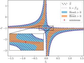
Figure 1: The submanifold $\widetilde{\mathcal{S}}$ of diagonal state-feedback stabilizing controllers ($K=\mathrm{diag}(l_{1},l_{2})$) for a $2\times 2$ system; superimposed with the level-sets of the constrained LQR cost ($h$), and the regions on which its Hessian is positive definite with respect to the inherent Riemannian geometry ($\operatorname{Hess}{h}$) and the Euclidean geometry ($\operatorname{\text{$\overline{\operatorname{Hess}}$}}{h}$), respectively. Note that $\widetilde{\mathcal{S}}$ is covered by the region on which $\operatorname{Hess}{h}\succ 0$. See Example 1 for more details.

Generally, the second order behavior of the cost function can be utilized in order to obtain a descent direction–as in the Newton method–as long as the Hessian stays positive definite. However, this second order information can be obtained in a variety of ways; for example, with respect to the usual Euclidean geometry (especially for linearly constrained problems) or more interestingly, with respect to the non-Euclidean geometry inherent to the cost function itself. A simple–yet relevant–example of the above statement is depicted in Figure 1 in relation to the set of diagonally constrained stabilizing controllers (denoted by $\widetilde{\mathcal{S}}$ )–which turns out to be non-convex even for this simple example consisting of two inputs and two states. More specifically, this set is the intersection of the 4-dimensional set of stabilizing controllers with a 2-dimensional plane defining the diagonal constraint. In reference to Figure 1, note how the Euclidean Hessian of the constrained LQR cost (denoted by $\operatorname{\text{$\overline{\operatorname{Hess}}$}}{h}$) is positive definite on a smaller subset of $\widetilde{\mathcal{S}}$ –especially in the vicinity of the “$\mathrm{minimum}$.” Therefore, one would expect that the neighborhood of $\mathrm{minimum}$ on which the Newton updates using the Euclidean geometry converge, be relatively small. In the meantime, if the second order behavior of the LQR cost is considered through the lens of Riemannian geometry, its Riemannian Hessian (denoted by $\operatorname{Hess}{h}$) captures the behavior of the cost function more effectively, in that it remains positive definite on a larger domain–compared with $\operatorname{\text{$\overline{\operatorname{Hess}}$}}{h}$. Hence, one expects a significant difference in the performance of second order optimization algorithms utilizing these two distinct geometries. To further expand on this example, one needs to define the (Riemannian) $\operatorname{Hess}{h}$ and devise a second order algorithm that iteratively optimize this constrained problem in the vicinity of a local optimum. This machinery is developed in the rest of this paper, after which we revisit the above example (see Example 1 in §6).

The literature on optimization over manifolds often relies on having access to either the exponential mapping [24, 25], or a retraction from its tangent bundle onto the manifold itself [26]. However, due to the intricate geometry of the manifold of Schur stabilizing controllers, the exponential mapping is computationally expensive and a suitable retraction is generally not available. Furthermore, many useful constraints for optimal LQR problems (such as OLQR or SLQR) inherit a linear structure. Hence, one may consider the Natural Gradient Descent approach of [27, 28] in order to utilize this inherent geometry; however, this approach is not directly applicable to more involved submanifolds of stabilizing controllers. Nonetheless, it is pertinent to ask whether we can still exploit the intrinsic non-Euclidean geometry–induced by, say, the quadratic cost and linear dynamics, in optimal control problems as illustrated in Figure 1– by circumventing the absence of a computationally feasible retraction while guaranteeing stability.

In this paper, we consider a general optimization problem over the set of linearly constrained stabilizing feedback gains; this setup can easily be tailored to other classes of constrained control synthesis problems. We introduce a Newton-type algorithm that utilizes both the inherent Riemannian geometry as well as the linear structure of the constraints, and provide its convergence analysis to the local minima. Here, in the absence of a computationally feasible (global) retraction from the tangent bundle to the manifold, we obtain the so-called stability certificate that–together with the linear structure of the constraints–substitute the role that a retraction would generally play, ensuring the feasibility of the next iterate. Finally, as the unit stepsize for the proposed iterates may not be possible in general, we guarantee a linear convergence rate–that eventually becomes quadratic as the iterates converge. Finally, we provide applications of the proposed methodology to the well-known state-feedback SLQR and OLQR problems, followed by numerical examples.

Our contributions can thus be summarized as follows: (i) We study the second order geometry of the manifold of stabilizing controllers induced by a pertinent Riemannian metric and its associated connection (a generalization of directional derivatives [29]), in order to obtain the second order information of a cost through defining the Riemannian Hessian. (ii) We provide extrinsic analysis for first and second-order behavior of a generic smooth cost function constrained to a Riemannian submanifold. This, in turn, allows for a general treatment of constrained optimization problems on the manifold of stabilizing controllers. (iii) We introduce Quasi Riemannian-Newton Policy Optimization (QRNPO) algorithm (pronounced as Kern PO) with convergence guarantees that exploits the inherent Riemannian geometry in the absence of the exponential mapping or a retraction, effectively providing a stability certificate for linearly constrained feedback gains. (iv) We apply our methodology to SLQR and OLQR problems by first, computing the second order behavior of the LQR cost with respect to the Riemannian connection, and then, explicating the solution to Newton equation for each case using this geometry. (v) While our approach allows for considering any choice of connection, here, we focus on the associated Riemannian connection–we also make a comparison to the ordinary Euclidean connection. (vi) Finally, we provide several numerical examples to showcase the performance and advantages of the proposed methodology that exploits the intrinsic geometry of constrained feedback stabilization. Further applications of the proposed algorithm–e.g. to the problem of controlling diffusion dynamics over a network–has recently appeared in [30].

The rest of the paper is organized as follows. In §2, we introduce the generic (stabilizing) feedback synthesis problem. We then provide the analysis of this problem through the lens of differential geometry in §3. In §4, we present the algorithm and its convergence analysis for optimization on submanifolds of stabilizing controllers. Applications to SLQR and OLQR problems are then presented in §5. Finally, numerical examples are provided in §6, followed by concluding remarks in §7. The appendix contains proofs of the results.
Notation: The space of $m\times n$ matrices over the reals is denoted by ${\text{M}(m\times n,\mathbb{R})}$ with the trivial smooth structure determined by the atlas consisting of the single chart $({\text{M}(m\times n,\mathbb{R})},\mathrm{vec})$, where $\mathrm{vec}\colon{\text{M}(m\times n,\mathbb{R})}\mapsto{\mathbb{R}}^{mn}$ denotes the operator that returns a vector obtained by (vertically) stacking the columns of a matrix–from left to right. We denote the transpose operator and the spectral norm of a matrix by $(\cdot)^{\intercal}$ and $\|\cdot\|_{2}$, respectively. The trace and spectral radius of a square matrix are denoted by $\mathrm{tr}\left[\cdot\right]$ and $\rho(\cdot)$. The Loewner partial order of symmetric positive (semi-)definite matrices is denoted by $\succ$ ($\succcurlyeq$); we use the same notation to denote positive (semi-)definiteness of 2-tensor fields. The maximum and minimum eigenvalues of symmetric matrices will be designated by $\operatorname{\text{$\overline{\lambda}$}}$ and $\operatorname{\text{$\underline{\lambda}$}}$, respectively. The set of positive integers less than or equal to $m$ is denoted by $[m]$. By ${\mathcal{M}}\coloneqq\left\{A\in{\text{M}(n\times n,\mathbb{R})}\;|\;\rho(A)<1\right\}$, we denote the set of (Schur) stable matrices, and define the Lyapunov map $\textstyle{\,\mathbb{L}}\colon{\mathcal{M}}\times{\text{M}(n\times n,\mathbb{R})}\mapsto{\text{M}(n\times n,\mathbb{R})},$ that sends the pair $(A,Z)$ to the unique solution $X$ of

$$X=AXA^{\intercal}+Z,$$ (1)

which has the representation $\textstyle X=\sum_{i=0}^{\infty}A^{i}Z(A^{\intercal})^{i}$; in this case, if $Z\succeq 0\,(\succ 0)$, then $X\succeq 0\,(\succ 0)$. Furthermore, when $Z\succeq 0$, then $X\succ 0$ if and only if $(A,Z^{1/2})$ is controllable (see [31] and references therein). For manifolds we follow the notation and results in [29] and [32] unless stated explicitly.

2 Problem Statement

Given a stabilizable pair $(A,B)$ with $A\in{\text{M}(n\times n,\mathbb{R})}$ and $B\in{\text{M}(n\times m,\mathbb{R})}$, we define

$$\mathcal{S}\coloneqq\{K\in{\text{M}(m\times n,\mathbb{R})}\;|\;\rho(A+BK)<1\},$$

as the set of stabilizing feedback gains. Subsequently, we will introduce a non-Euclidean geometry over $\mathcal{S}$ using a metric arising naturally in the context of optimal control problems. We are often interested in feedback gains $K$ that lie in a relatively simple subset ${\mathcal{K}}$ of ${\text{M}(m\times n,\mathbb{R})}$, such that $\scalebox{0.9}{$\widetilde{\mathcal{S}}$}\coloneqq{\mathcal{K}}\cap\mathcal{S}$ is an embedded submanifold of $\mathcal{S}$ (see §3.1). A common example of this would be a linear subspace of ${\text{M}(m\times n,\mathbb{R})}$ characterizing a prescribed sparsity pattern for the admissible controller gains (see §5.1.2). Another example is the optimal output-feedback synthesis considered in §5.1.3.

Herein, we are concerned with the optimization problem,

$$\displaystyle\min_{K}f(K)\qquad\text{s.t. }\quad K\in\scalebox{0.9}{$\widetilde{\mathcal{S}}$},$$ (2)

where $f\in{C^{\infty}(\mathcal{S},\mathbb{R})=C^{\infty}(\mathcal{S})}$ and $\widetilde{\mathcal{S}}$ is an embedded submanifold of $\mathcal{S}$, especially when it is endowed with a linear structure. This problem is motivated by parameterized feedback synthesis problems where we optimize the LQR cost $f$ directly for the policy $K\in\scalebox{0.9}{$\widetilde{\mathcal{S}}$}$ which takes the form of $f(K)=\frac{1}{2}\mathrm{tr}\left[P_{K}\Sigma_{K}\right]$ with some $\Sigma_{K},P_{K}\succ 0$ smoothly depending on $K$ (see §5 for further details).

Our approach involves using this linear structure with an appropriate Riemannian geometry of $\mathcal{S}$ to circumvent the absence of a (computationally feasible) global retraction from $T\mathcal{S}$ onto $\mathcal{S}$ (or $\widetilde{\mathcal{S}}$ )–due to the intricate geometry of $\mathcal{S}$. In this paper, we do not explicitly discuss conditions for the existence of the local (or global) optima for equation 2; as such, we assume that the minimum exists; see [33, 34] for a few relevant applications.

In order to handle a generic embedded submanifold $\widetilde{\mathcal{S}}$ , we study the behavior of the restricted function $h\coloneqq f|_{\footnotesize\scalebox{0.9}{$\widetilde{\mathcal{S}}$}}$ from an extrinsic point of view, an approach that can be generalized to any such submanifold. We note that in general, the function $f$ is not convex and the constraint submanifold $\widetilde{\mathcal{S}}$ might be disconnected. Thus, here we focus on local convergence results that aim to exploit the inherent geometry of the problem in order to achieve fast convergence rates–with a relatively reasonable computational complexity.

3 Geometry of the Synthesis Problem

In order to examine equation 2, we analyze the domain manifold using machinery borrowed from differential geometry. Note that embedded submanifolds $\widetilde{\mathcal{S}}$ endowed with a linear structure can certainly be investigated without using such a machinery. However, neither the corresponding results can be generalized to submanifolds with nonlinear structures, nor the geometry induced by the cost function can be exploited for developing the corresponding optimization algorithms.

Before we proceed, it is worth noting that if we were to directly apply the results developed for optimization over the manifolds (such as [26]), it would have been necessary to access a retraction from the tangent bundle $T\scalebox{0.9}{$\widetilde{\mathcal{S}}$}$ onto $\widetilde{\mathcal{S}}$ . Unfortunately, due to the intricate geometry of $\mathcal{S}$, such a mapping is generally not available. Additionally, we will see that the Riemannian exponential map, with respect to the inherent geometry associated with optimal control problems, involves a system of ordinary differential equations whose coefficients are solutions to different Lyapunov equations. Therefore, even though it is possible to compute the exponential mapping, in general, its computational overhead is hard to justify. Nonetheless, we show how we can circumvent this issue when the Riemannian tangential projection onto $T\scalebox{0.9}{$\widetilde{\mathcal{S}}$}$ is available–an operation that is more streamlined.

3.1 Analysis of the domain manifold

It is known that $\mathcal{S}$ is contractible [35], and unbounded when $m\geq 2$ with the topological boundary $\partial\mathcal{S}=\{K\in{\text{M}(m\times n,\mathbb{R})}\;|\;\rho(A+BK)=1\}$ as a subset of ${\text{M}(m\times n,\mathbb{R})}$. Furthermore, $\mathcal{S}$ is open in ${\text{M}(m\times n,\mathbb{R})}$ (by continuity of eigenvalues in the entries of the matrix [36, Theorem 5.2] and passing to the quotient [37, Theorem 3.73]); as such $\mathcal{S}$ is a submanifold without boundary.

In this paper we focus on $\mathcal{S}$ as a manifold on its own. Note that $\mathcal{S}$ can be covered by a single smooth chart and the tangent bundle of $\mathcal{S}$, denoted by $T\mathcal{S}$, is diffeomorphic to $\mathcal{S}\times{\mathbb{R}}^{mn}$, which in turn is diffeomorphic to $\mathcal{S}\times{\text{M}(m\times n,\mathbb{R})}$ under the map $\mathrm{Id}_{\mathcal{S}}\times\mathrm{vec}^{-1}$. We refer to this composition of diffeomorphisms as the usual identification of the tangent bundle (or $T_{K}S\cong{\text{M}(m\times n,\mathbb{R})}$ at any point $K\in\mathcal{S}$) if we need to identify any element of $T\mathcal{S}$ (or $T_{K}\mathcal{S}$). In particular, let us denote the coordinates of this global chart by $(x^{i,j})$ for $\mathcal{S}$, its associated global coordinate frame by $(\frac{\partial}{\partial x^{i,j}})$ or simply $(\partial_{i,j})$, and its dual coframe by $(dx^{i,j})$, where $i=1,\dots,m$ and $j=1,\dots,n$. Moreover, the $(k,\ell)$th element of any matrix $A\in{\text{M}(m\times n,\mathbb{R})}$ is denoted by $[A]_{k,\ell}$ or $[A]^{k,\ell}$ depending on viewing $A$ as a point or a tangent vector, respectively. Then, for example, under the usual identification of tangent bundle, for any fixed $i$ and $j$, we identify $\partial_{i,j}$ as a matrix in ${\text{M}(m\times n,\mathbb{R})}$ whose elements are $[\partial_{i,j}]^{k,\ell}=1$ if $k=i$ and $\ell=j$, and otherwise $[\partial_{i,j}]^{k,\ell}=0$. We also use the Einstein summation convention as explained in [29] for double indices; for example, we write $x^{i,j}\partial_{i,j}$ to denote $\sum_{i=1}^{m}\sum_{j=1}^{n}x^{i,j}\partial_{i,j}$. A vector field $V$ on $\mathcal{S}$ is a smooth map $V\colon\mathcal{S}\mapsto T\mathcal{S}$, usually written as $K\mapsto V_{K}$, with the property that $V_{K}\in T_{K}\mathcal{S}$ for all $K\in\mathcal{S}$. A covariant 2-tensor field is a smooth real-valued multilinear function of 2 vector fields. We denote the set of all vector fields over $\mathcal{S}$ by $\mathfrak{X}(\mathcal{S})$, and the bundle of covariant 2-tensor fields on $\mathcal{S}$ by $T^{2}(T^{*}\mathcal{S})$. Finally, for any general mapping $P\colon\mathcal{S}\mapsto\star$, we use $P_{K},P|_{K}$ or $P(K)$ to denote the element in $\star$ that $K\in\mathcal{S}$ has been mapped to. The following is a frequently used technical lemma.

Lemma 3.1.

The subset ${\mathcal{M}}$ is an open submanifold of ${\text{M}(n\times n,\mathbb{R})}$, the Lyapunov map ${\,\mathbb{L}}\colon{\mathcal{M}}\times{\text{M}(n\times n,\mathbb{R})}\mapsto{\text{M}(n\times n,\mathbb{R})}$ is smooth, and its differential acts as

$$\operatorname{\mathrm{d}}{\,\mathbb{L}}_{(A,Q)}[E,F]={\,\mathbb{L}}\big{(}A,E{\,\mathbb{L}}(A,Q)A^{\intercal}+A{\,\mathbb{L}}(A,Q)E^{\intercal}+F\big{)}$$

on any $(E,F)\in T_{(A,Q)}({\mathcal{M}}\times{\text{M}(n\times n,\mathbb{R})})$ with the identification that follows by $T_{(A,Q)}({\mathcal{M}}\times{\text{M}(n\times n,\mathbb{R})})\cong T_{A}{\mathcal{M}}\oplus T_{Q}{\text{M}(n\times n,\mathbb{R})}\cong{\text{M}(n\times n,\mathbb{R})}\oplus{\text{M}(n\times n,\mathbb{R})}$. Furthermore, for any $A\in{\mathcal{M}}$ and $Q,\Sigma\in{\text{M}(n\times n,\mathbb{R})}$ we have, the so-called Lyapunov-trace  property,

$$\mathrm{tr}\left[{\,\mathbb{L}}(A^{\intercal},Q)\Sigma\right]=\mathrm{tr}\left[{\,\mathbb{L}}(A,\Sigma)Q\right].$$

Next, we note (see equation 9 in §5) that many optimal control problems such as SLQR, OLQR and even Linear Quadratic Gaussian (LQG) share a similar cost structure, as $\textstyle f(K)=\frac{1}{2}\mathrm{tr}\left[P_{K}\Sigma_{K}\right],$ where mappings $P,\Sigma\colon\mathcal{S}\mapsto{\text{M}(n\times n,\mathbb{R})}$ send $K$ to

$$P_{K}\coloneqq{\,\mathbb{L}}(A_{\mathrm{cl}}^{\intercal},Q+K^{\intercal}RK),\quad\Sigma_{K}\coloneqq\Sigma_{1}+K^{\intercal}\Sigma_{2}K,$$ (3)

respectively, with the closed-loop system $A_{\mathrm{cl}}\coloneqq A+BK$, and $\Sigma_{1},\Sigma_{2}\succeq 0$ as prescribed matrices with appropriate dimensions. By the Lyapunov-trace property, the cost can be recast as $f(K)=\frac{1}{2}\mathrm{tr}\left[(Q+K^{\intercal}RK){\,\mathbb{L}}(A_{\mathrm{cl}},\Sigma_{K})\right]$. Motivated by this, we define a covariant 2-tensor field on $\mathcal{S}$ which will subsequently be proved to be a Riemannain metric. Riemannian metrics have been used in the literature to efficiently capture the geometry of the problem; e.g., see [39] for optimizing the Rayleigh quotient on the Grassmann manifold, and [40] for natural policy gradient on Markov decision processes. Note that our metric is different from the “Hessian metric” induced by, say, a convex function [41].

Lemma 3.2.

Let $\left\langle\cdot,\cdot\right\rangle\colon\mathfrak{X}(\mathcal{S})\times\mathfrak{X}(\mathcal{S})\mapsto C^{\infty}(\mathcal{S})$ denote the mapping that, under the usual identification of the tangent bundle, for any $V,W\in\mathfrak{X}(\mathcal{S})$ sets,

$$\left\langle V,W\right\rangle\big{|}_{K}\coloneqq\mathrm{tr}\left[(V_{K})^{\intercal}\;W_{K}\;{\,\mathbb{L}}(A_{\mathrm{cl}},\Sigma_{K})\right],\quad\forall K\in\mathcal{S}.$$

Then this map, induced by a smooth symmetric covariant 2-tensor field, is well-defined.

Now, let $g\colon\mathcal{S}\mapsto T^{2}(T^{*}\mathcal{S})$ be a smooth section of the bundle $T^{2}(T^{*}\mathcal{S})$ that sends $K$ to $\left\langle\cdot,\cdot\right\rangle\big{|}_{K}$. Then, $g$ is in fact a Riemannian metric under mild conditions formalized below.

Proposition 3.3.

If $(A_{\mathrm{cl}},\Sigma_{K}^{1/2})$ is controllable and for all $K\in\mathcal{S}$, $\Sigma_{K}~{}\succeq~{}0$, then $(\mathcal{S},g)$ is a Riemannian manifold. Moreover, if we define the mapping $Y\colon\mathcal{S}\mapsto{\text{M}(n\times n,\mathbb{R})}$ sending $K$ to

$$Y_{K}\coloneqq{\,\mathbb{L}}(A_{\mathrm{cl}},\Sigma_{K}),$$

then, with respect to the dual coframe $(dx^{i,j})$, $g=g_{(i,j)(k,\ell)}dx^{i,j}\otimes dx^{k,\ell}$, where each $g_{(i,j)(k,\ell)}\in C^{\infty}(\mathcal{S})$ satisfies $g_{(i,j)(k,\ell)}(K)=[Y_{K}]_{\ell,j}$ if $i=k$, and $0$ otherwise. Furthermore, the inverse matrix $g^{(i,j)(k,\ell)}$ satisfies $g^{(i,j)(k,\ell)}(K)=[Y_{K}^{-1}]_{\ell,j}$ if $i=k$, and $0$ otherwise.

Remark 1.

The premise of Proposition 3.3 is satisfied if $\Sigma_{K}\succ 0$ for all $K\in\mathcal{S}$; e.g., when $\Sigma_{1}\succ 0$ and $\Sigma_{2}\succeq 0$. Also, by some algebraic manipulations, the well-known Hewer’s algorithm [42] can be viewed as a Riemannian quasi-Newton iteration with respect to this Riemannian metric but with the Euclidean connection–also see Remark 5. Finally, we remark that the developed machinery can be generalized by modifying the Riemannian metric to incorporate a “preconditioning” positive definite $\Theta\succ 0$ such as:

$$\left\langle V,W\right\rangle\big{|}_{K}\coloneqq\mathrm{tr}\left[(V_{K})^{\intercal}\;\Theta\;W_{K}\;{\,\mathbb{L}}(A_{\mathrm{cl}},\Sigma_{K})\right],\quad\forall K\in\mathcal{S}.$$

In this case, a judicious choice of $\Theta$ may, in general, improve the performance of corresponding numerical schemes. This metric also has a system theoretic interpretation that will be elaborated upon in our subsequent works.

3.1.1 Riemannian connection on $T\mathcal{S}$

First, consider a Riemannian submanifold $(\scalebox{0.9}{$\widetilde{\mathcal{S}}$},\scalebox{0.9}{$\widetilde{g}$})$ with $\scalebox{0.9}{$\widetilde{g}$}\coloneqq\iota^{*}_{\footnotesize\scalebox{0.9}{$\widetilde{\mathcal{S}}$}}g$, where $\iota^{*}_{\footnotesize\scalebox{0.9}{$\widetilde{\mathcal{S}}$}}$ denotes the pull-back by inclusion. In order to understand the second order behavior–i.e., the Hessian–of a smooth function on $\widetilde{\mathcal{S}}$ , we need to study the notion of connection in $T\mathcal{S}$, and how it relates to analogous construct in the tangent bundle $T\scalebox{0.9}{$\widetilde{\mathcal{S}}$}$–see [29] for further details. Recall that by Fundamental Theorem of Riemannian Geometry, there exists a unique connection $\nabla\colon\mathfrak{X}(\mathcal{S})\times\mathfrak{X}(\mathcal{S})\mapsto\mathfrak{X}(\mathcal{S})$ in $T\mathcal{S}$ that is compatible with $g$ and symmetric, i.e., for all $U,V,W\in\mathfrak{X}(\mathcal{S})$ we have:

• $\nabla_{U}\left\langle V,W\right\rangle=\left\langle\nabla_{U}V,W\right\rangle+\left\langle V,\nabla_{U}W\right\rangle$,

• $\nabla_{U}V-\nabla_{V}U\equiv[U,V]$,

where $[V,W]\in\mathfrak{X}(\mathcal{S})$ denotes the Lie bracket of $V$ and $W$.

Note that, the restriction of $\nabla$ to $\mathfrak{X}(\scalebox{0.9}{$\widetilde{\mathcal{S}}$})\times\mathfrak{X}(\scalebox{0.9}{$\widetilde{\mathcal{S}}$})$ would not be a connection in $T\scalebox{0.9}{$\widetilde{\mathcal{S}}$}$ as its range does not necessary lie in $\mathfrak{X}(\scalebox{0.9}{$\widetilde{\mathcal{S}}$})$. However, we can denote the (Riemannian) tangential and normal projections by $\operatorname{\pi^{\top}}\colon T\mathcal{S}|_{\footnotesize\scalebox{0.9}{$\widetilde{\mathcal{S}}$}}\mapsto T\scalebox{0.9}{$\widetilde{\mathcal{S}}$}$ and $\operatorname{\pi^{\perp}}\colon T\mathcal{S}|_{\footnotesize\scalebox{0.9}{$\widetilde{\mathcal{S}}$}}\mapsto N\scalebox{0.9}{$\widetilde{\mathcal{S}}$}$, respectively, with $N\scalebox{0.9}{$\widetilde{\mathcal{S}}$}$ indicating the normal bundle of $\widetilde{\mathcal{S}}$ . Then, by Gauss Formula, if $\widetilde{\nabla}\colon\mathfrak{X}(\scalebox{0.9}{$\widetilde{\mathcal{S}}$})\times\mathfrak{X}(\scalebox{0.9}{$\widetilde{\mathcal{S}}$})\mapsto\mathfrak{X}(\scalebox{0.9}{$\widetilde{\mathcal{S}}$})$ denotes the Riemannian connection in the tangent bundle $T\scalebox{0.9}{$\widetilde{\mathcal{S}}$}$, computed via,

$$\widetilde{\nabla}_{U}V=\operatorname{\pi^{\top}}\nabla_{U}V,$$ (4)

for any $U,V\in\mathfrak{X}(\scalebox{0.9}{$\widetilde{\mathcal{S}}$})$ arbitrarily extended to vector fields on a neighborhood of $\widetilde{\mathcal{S}}$ in $\mathcal{S}$.

For computational purposes, we also obtain the Christoffel symbols associated with $g$ (denoted by $\Gamma^{(i,j)}_{(k,\ell)(p,q)}$) in the global coordinate frame. This would, in turn, completely characterize the connection $\nabla$ and facilitates its computation in this frame.

Proposition 3.4.

Consider a point $K\in\mathcal{S}$ and, under the usual identification of $T\mathcal{S}$, define

$$\begin{aligned} dY_{K}{(p,q)}\coloneqq{\,\mathbb{L}}\big{(}A_{\mathrm{cl}},\;&B\partial_{(p,q)}Y_{K}A_{\mathrm{cl}}^{\intercal}+A_{\mathrm{cl}}Y_{K}\partial_{(p,q)}^{\intercal}B^{\intercal}\\ &+\partial_{(p,q)}^{\intercal}\Sigma_{2}K+K^{\intercal}\Sigma_{2}\partial_{(p,q)}\big{)}\end{aligned}$$

for each $(p,q)\in[m]\times[n]$ where $Y_{K}={\,\mathbb{L}}(A_{\mathrm{cl}},\Sigma_{K})$. Then, the Christoffel symbols associated with the metric $g$ in the global coordinate frame $(\partial_{(i,j)})$ satisfies $\Gamma^{(i,j)}_{(k,\ell)(p,q)}(K)=$

$$\begin{cases}\nicefrac{{1}}{{2}}\left[dY_{K}{(p,q)}\,Y_{K}^{-1}\right]_{(\ell,j)},&\text{if $k=i\neq p$,}\\ \nicefrac{{1}}{{2}}\left[dY_{K}{(k,\ell)}\,Y_{K}^{-1}\right]_{(q,j)},&\text{if $p=i\neq k$,}\\ \textstyle-\nicefrac{{1}}{{2}}\sum_{s}\left[dY_{K}{(i,s)}\right]_{(q,\ell)}[Y_{K}^{-1}]_{(s,j)},&\text{if $p=k\neq i$,}\\ \textstyle\nicefrac{{1}}{{2}}\sum_{s}\big{(}\left[dY_{K}{(i,\ell)}\right]_{(q,s)}+\left[dY_{K}{(i,q)}\right]_{(\ell,s)}&\\ \qquad\quad-\left[dY_{K}{(i,s)}\right]_{(q,\ell)}\big{)}\;[Y_{K}^{-1}]_{(s,j)},&\text{if $p=k=i$,}\\ 0,&\text{otherwise.}\end{cases}$$

Remark 2.

Note that with respect to the global coordinates of $(\mathcal{S},g,\nabla)$, the geodesic equation is a system of $(mn)$ second-order ordinary differential equations whose varying coefficients involve $(mn)^{3}$ Christoffel symbols $\Gamma^{(i,j)}_{(i,\ell)(i,q)}$ as obtained above. Therefore, computing the Riemannian Exponential mapping is computationally burdensome; as such, in this work, we avoid using it as a retraction.

3.2 Extrinsic analysis of a smooth function constrained on a Riemannian submanifold

In this subsection, we study the gradient and Hessian operators of a constrained smooth function from an extrinsic point of view, which is yet to be defined. In other words, we consider $(\scalebox{0.9}{$\widetilde{\mathcal{S}}$},\scalebox{0.9}{$\widetilde{g}$})$ as a Riemannian submanifold of $(\mathcal{S},g)$, where $\scalebox{0.9}{$\widetilde{g}$}=\iota_{\footnotesize\scalebox{0.9}{$\widetilde{\mathcal{S}}$}}^{*}g$, with $\iota_{\footnotesize\scalebox{0.9}{$\widetilde{\mathcal{S}}$}}^{*}$ denoting the pull-back by inclusion of $\widetilde{\mathcal{S}}$ into $\mathcal{S}$. Then, by considering any smooth function $f$ on $\mathcal{S}$, we can define its restriction to $\widetilde{\mathcal{S}}$ as

$$h\coloneqq f|_{\footnotesize\scalebox{0.9}{$\widetilde{\mathcal{S}}$}},$$

and examine how its gradient and Hessian operators are related to those of $f$. In order to answer this question, we utilize the Riemannian connection to analyze the second order behavior of $f$ (or that of $h$).

First, recall from [29] that the gradient of $f$ with respect to the Riemannian metric $g$, denoted by $\operatorname{grad}{f}\in\mathfrak{X}(\mathcal{S})$, is the unique vector field satisfying

$$\left\langle V,\operatorname{grad}{f}\right\rangle=Vf,$$

for any $V\in\mathfrak{X}(\mathcal{S})$. Then, we denote the Hessian operator of $f\in C^{\infty}(\mathcal{S})$ as the map $\operatorname{Hess}{f}\colon\mathfrak{X}(\mathcal{S})\mapsto\mathfrak{X}(\mathcal{S})$ defined by

$$\operatorname{Hess}{f}[U]\coloneqq\nabla_{U}\operatorname{grad}{f},$$

for any $U\in\mathfrak{X}(\mathcal{S})$. Note that we use the same notation to denote the gradient and Hessian operators defined on the submanifold $\widetilde{\mathcal{S}}$ (see the appendix). Finally, for any normal vector field $N$ (i.e., a smooth section of $N\scalebox{0.9}{$\widetilde{\mathcal{S}}$}$), the Weingarten map in the direction of $N$ is a self-adjoint linear map denoted by $\mathbb{W}_{N}\colon\mathfrak{X}(\scalebox{0.9}{$\widetilde{\mathcal{S}}$})\mapsto\mathfrak{X}(\scalebox{0.9}{$\widetilde{\mathcal{S}}$})$, which defines a smooth bundle homomorphism from $T\scalebox{0.9}{$\widetilde{\mathcal{S}}$}$ to itself (linear on each tangent space), characterized by [29],

$$\left\langle\mathbb{W}_{N}[V],W\right\rangle=\left\langle N,\operatorname{\pi^{\perp}}(\nabla_{V}W)\right\rangle,\quad\forall V,W\in\mathfrak{X}(\mathcal{S}).$$

Now, we can formalize this abstract extrinsic analysis as follows.

Proposition 3.5.

Suppose $\widetilde{\mathcal{S}}$ is an embedded Riemannian submanifold of $\mathcal{S}$, both equipped with their respective Riemannian connections. Let $f\in C^{\infty}(\mathcal{S})$ be any smooth function; then $h\coloneqq f|_{\footnotesize\scalebox{0.9}{$\widetilde{\mathcal{S}}$}}$ is smooth on $\widetilde{\mathcal{S}}$ and we have

$$\operatorname{grad}{h}=\operatorname{\pi^{\top}}(\operatorname{grad}{f}|_{\footnotesize\scalebox{0.9}{$\widetilde{\mathcal{S}}$}}).$$

Furthermore, under the usual identification of $T\scalebox{0.9}{$\widetilde{\mathcal{S}}$}\subset T\mathcal{S}$, for any $V\in\mathfrak{X}(\scalebox{0.9}{$\widetilde{\mathcal{S}}$})$ we have,

$$\operatorname{Hess}{h}[V]=\operatorname{\pi^{\top}}(\operatorname{Hess}{f}[V]\big{|}_{\footnotesize\scalebox{0.9}{$\widetilde{\mathcal{S}}$}})+\mathbb{W}_{\operatorname{\pi^{\perp}}(\operatorname{grad}{f}|_{\footnotesize\scalebox{0.9}{$\widetilde{\mathcal{S}}$}})}[V],$$

where $V$ is arbitrarily extended to vector fields on a neighborhood of $\widetilde{\mathcal{S}}$ in $\mathcal{S}$.

3.2.1 On the choice of connection

On the manifold $(\mathcal{S},g,\nabla)$, computing the exponential map requires finding solution to a system of ordinary differential equations of dimension $mn$. This approach is not only computationally demanding but also does not necessarily provide an exponential map of the submanifold $\widetilde{\mathcal{S}}$ (unless it happens to be totally geodesic). In order to avoid the computation of the Riemannian exponential map, it seems reasonable to perform updates by using simpler retractions from the tangent bundle to the manifold (cf. [26]); however, in general, we do not have access to such a retraction in our setup. Another computational overhead of utilizing the Riemannian connection associated with the Riemannian metric $g$ pertains to the $(mn)$-number of Lyapunov equations involved in obtaining the Christoffel symbols at each point.

On the other hand, for applications in which the submanifold appears as $\scalebox{0.9}{$\widetilde{\mathcal{S}}$}=\mathcal{S}\cap{\mathcal{K}}$, where ${\mathcal{K}}$ is an affine subspace of ${\text{M}(m\times n,\mathbb{R})}$, it might seem reasonable to consider the ambient manifold $(\mathcal{S},g,\overline{\nabla})$, where $\overline{\nabla}$ refers to the so-called Euclidean connection, i.e., the connection whose symbols (with respect to the global coordinates) all vanish (i.e., $\overline{\Gamma}^{i,j}_{(k,\ell)(p,q)}\equiv 0$ on $\mathcal{S}$). This results in a simpler Hessian operator which, however, does not respect the geometry of $(\mathcal{S},g)$ simply because $\overline{\nabla}$ is not compatible with the metric $g$–in contrast to its associated Riemannian connection. Nonetheless, for completeness, we also define the Euclidean Hessian operator of $f\in C^{\infty}(\mathcal{S})$ as the map $\operatorname{\text{$\overline{\operatorname{Hess}}$}}{f}\colon\mathfrak{X}(\mathcal{S})\mapsto\mathfrak{X}(\mathcal{S})$ defined by

$$\operatorname{\text{$\overline{\operatorname{Hess}}$}}{f}[U]\coloneqq\overline{\nabla}_{U}\operatorname{grad}{f},$$

for any $U\in\mathfrak{X}(\mathcal{S})$. This operator enjoys similar properties as that of $\operatorname{Hess}{f}$, but contains different second order information about $f$ (e.g., see Figure 1 for a comparison).

4 Riemannian Optimization on Submanifolds of $\mathcal{S}$ with Linear Structure

In this section, we propose an optimization algorithm for smooth cost functions, constrained to submanifolds of $\mathcal{S}$ that are endowed with a linear structure; that is, $\scalebox{0.9}{$\widetilde{\mathcal{S}}$}=\mathcal{S}\cap{\mathcal{K}}$, where ${\mathcal{K}}$ entails a linear structure in ${\text{M}(m\times n,\mathbb{R})}$. The proposed algorithm, does not involve the exponential mapping (due to its computational complexity); note that no other retraction from the tangent space onto the manifold $\mathcal{S}$ is known. Instead, we exploit this linear structure together with a geometrically-induced stability certificate that guarantees stability of the iterates by adjusting the respective stepsize.

In what follows, we first introduce this stability certificate and then propose the algorithm. We then show how this certificate can be utilized to choose stepsizes that guarantee a linear convergence rate; furthermore, we will discuss existence of neighborhoods–containing a local minima–on which the algorithm achieves a quadratic rate of convergence.

4.0.1 Stability certificate and (direct) policy optimization

Recall that $\mathcal{S}$ is open in ${\text{M}(m\times n,\mathbb{R})}$. Nonetheless, we provide the following result that quantifies this fact with respect to the problem parameters; an observation that has an immediate utility for analyzing iterative algorithms on $\mathcal{S}$.

Lemma 4.1.

Consider a smooth mapping $\mathcal{Q}\colon\mathcal{S}\mapsto{\text{M}(n\times n,\mathbb{R})}$ that sends $K$ to any $\mathcal{Q}_{K}\succ 0$. For any direction $G\in T_{K}\mathcal{S}\cong{\text{M}(m\times n,\mathbb{R})}$ at any point $K\in\mathcal{S}$, if

$$0\leq\eta\leq s_{K}\coloneqq\Large\nicefrac{{\operatorname{\text{$\underline{\lambda}$}}(\mathcal{Q}_{K})}}{{\left(2\operatorname{\text{$\overline{\lambda}$}}\left({\,\mathbb{L}}(A_{\mathrm{cl}}^{\intercal},\mathcal{Q}_{K})\right)\|BG\|_{2}\right)}},$$

then $K^{+}\coloneqq K+\eta G\in\mathcal{S}$; $s_{K}$ will be referred to as the stability certificate at $K$.

• As $K$ is stabilizing, for any such $\mathcal{Q}_{K}$, there exists a matrix $P={\,\mathbb{L}}(A_{\mathrm{cl}}^{\intercal},\mathcal{Q}_{K})\succ 0$ satisfying $P=A_{\mathrm{cl}^{+}}^{\intercal}PA_{\mathrm{cl}^{+}}+L$ with $A_{\mathrm{cl}^{+}}\coloneqq A+BK^{+}$ and $L\coloneqq\mathcal{Q}_{K}+A_{\mathrm{cl}}^{\intercal}PA_{\mathrm{cl}}-A_{\mathrm{cl}^{+}}^{\intercal}PA_{\mathrm{cl}^{+}}$. Therefore, in order to establish that $K^{+}$ is stabilizing, as $P\succ 0$–by the Lyapunov Stability Criterion [43, Theorem8.4]–it suffices to show that $L\succ 0$. Next,

  $$L= \mathcal{Q}_{K}-\eta G^{\intercal}B^{\intercal}PA_{\mathrm{cl}}-\eta A_{\mathrm{cl}}^{\intercal}PBG-\eta^{2}G^{\intercal}B^{\intercal}PBG$$

  $$\succcurlyeq \mathcal{Q}_{K}-aA_{\mathrm{cl}}^{\intercal}PA_{\mathrm{cl}}-(1+{\large\nicefrac{{1}}{{a}}})\eta^{2}G^{\intercal}B^{\intercal}PBG$$

  $$= (1+a)\mathcal{Q}_{K}-aP-(1+{\large\nicefrac{{1}}{{a}}})\eta^{2}G^{\intercal}B^{\intercal}PBG,$$ (5)

  because for any $a>0$, $P\succ 0$ implies

  $$aA_{\mathrm{cl}}^{\intercal}PA_{\mathrm{cl}}+({\large\nicefrac{{\eta^{2}}}{{a}}})G^{\intercal}B^{\intercal}PBG\succcurlyeq\eta G^{\intercal}B^{\intercal}PA_{\mathrm{cl}}+\eta A_{\mathrm{cl}}^{\intercal}PBG.$$

  Now, by recalling the infinite-sum representation of $P$ and the fact that $\mathcal{Q}_{K}\succeq 0$, we conclude that $\operatorname{\text{$\overline{\lambda}$}}(P)\geq\operatorname{\text{$\overline{\lambda}$}}(\mathcal{Q}_{K})\geq\operatorname{\text{$\underline{\lambda}$}}(\mathcal{Q}_{K})$. Then, we proceed as follows: if $\operatorname{\text{$\overline{\lambda}$}}(P)>\operatorname{\text{$\underline{\lambda}$}}(\mathcal{Q}_{K})$ then we choose $a=\Large\nicefrac{{\operatorname{\text{$\underline{\lambda}$}}(\mathcal{Q}_{K})}}{{(2\operatorname{\text{$\overline{\lambda}$}}(P)-2\operatorname{\text{$\underline{\lambda}$}}(\mathcal{Q}_{K}))}}>0$; otherwise, we choose $a>2\eta^{2}\|BG\|_{2}^{2}$. Either way, by comparing the minimum eigenvalues of both sides in equation 5,

  $$\operatorname{\text{$\underline{\lambda}$}}(L)\geq\operatorname{\text{$\underline{\lambda}$}}(\mathcal{Q}_{K})/2-\left[{\large\nicefrac{{2\operatorname{\text{$\overline{\lambda}$}}(P)^{2}}}{{\operatorname{\text{$\underline{\lambda}$}}(\mathcal{Q}_{K})}}}-\operatorname{\text{$\overline{\lambda}$}}(P)\right]\eta^{2}\|BG\|_{2}^{2}.$$

  Therefore, if $|\eta|\leq\Large\nicefrac{{\operatorname{\text{$\underline{\lambda}$}}(\mathcal{Q}_{K})}}{{(2\operatorname{\text{$\overline{\lambda}$}}(P)\|BG\|_{2})}}$, then $L\succ 0$, hence completing the proof. ∎

Remark 3.

The proceeding lemma also provides a conditioning of the optimization problem in terms of system parameters $A,B$. In other words, for any choice of $\mathcal{Q}_{K}\succ 0$ at any $K\in\mathcal{S}$, the ratio ${\operatorname{\text{$\overline{\lambda}$}}\left({\,\mathbb{L}}(A_{\mathrm{cl}}^{\intercal},\mathcal{Q}_{K})\right)}/{\operatorname{\text{$\underline{\lambda}$}}(\mathcal{Q}_{K})}$ represents a condition number revealing geometric information on the manifold at $K$. In a sense, this ratio reflects the Riemannian curvature of $(\mathcal{S},g,\nabla)$; this connection will be further explored in our future work.

Next, we propose an algorithm with convergence guarantees with at least a linear rate (when the iterates are far from the local optima) and eventually a Q-quadratic rate (when the iterates are close enough to the local optima). The complication here is that we do not have access to a retraction with a reasonable computational complexity (see Remark 2). We claim that, starting close enough to a local minimum, a Newton-type method using Riemannian metric and the Euclidean/Riemannian connection must converge quadratically if one could have used the stepsize $\eta=1$. This is in fact due to the exponential mapping with respect to the Euclidean connection that serves as a retraction with desirable properties. However, the stability certificate suggests that at least away from the local minimum, it might not be possible to use such a large stepsize. Therefore, a stepsize rule has to be deduced–that in turn, hinges upon the stability certificate; the resulting algorithm is summarized in Algorithm 1. Hereafter, we refer to the solution $G\in T_{K}\scalebox{0.9}{$\widetilde{\mathcal{S}}$}$ of the following equation as the Newton direction on $\widetilde{\mathcal{S}}$ :

$$\operatorname{Hess}{h}_{K}[G]=-\operatorname{grad}{h}_{K},$$

where $h=f|_{\footnotesize\scalebox{0.9}{$\widetilde{\mathcal{S}}$}}$; similarly, when $\operatorname{Hess}{h}$ is replaced by $\operatorname{\text{$\overline{\operatorname{Hess}}$}}{h}$, the corresponding solution is referred to as the Euclidean Newton direction.

1:Initialization: Problem parameters $(A,B)$,
the linear constraint ${\mathcal{K}}$ and an initial feasible stabilizing controller $K_{0}\in\scalebox{0.9}{$\widetilde{\mathcal{S}}$}=\mathcal{S}\cap{\mathcal{K}}$

2:Choose a smooth mapping $K\mapsto\mathcal{Q}_{K}\succ 0$; set $t=0$

3:Until stopping criteria are met, do

4:      Find the Newton direction $G_{t}$ on

$\widetilde{\mathcal{S}}$

satisfying

$$\operatorname{Hess}{h}_{K_{t}}[G_{t}]=-\operatorname{grad}{h}_{K_{t}}$$

5:      Use $\mathcal{Q}_{K_{t}}$ to obtain a stability certificate $s_{K_{t}}$

6:      Compute step-size $\eta_{t}=\min\left\{s_{K_{t}},1\right\}$

7:      Update: $K_{t+1}=K_{t}+\eta_{t}G_{t}$

8:      $t\leftarrow t+1$

Algorithm 1 Quasi Riemannian-Newton Policy Optimization (QRNPO) for Constrained Problems on $\mathcal{S}$

4.0.2 Linear-quadratic convergence of QRNPO

In this section, we establish the local linear-quadratic convergence of QRNPO on the submanifold $\widetilde{\mathcal{S}}$ using differential geometric techniques [29, 26, 24]. Herein, avoiding the exponential map induced by the Riemannian connection for updating the iterates, and instead relying the stability certificate, adds another layer of complications for the convergence analysis. To proceed, we say that $K^{*}$ is a critical point of $h$ if $\operatorname{grad}{h}_{K^{*}}=0$; it is nondegenerate if $\operatorname{Hess}{h}_{K^{*}}$ is nondegenerate, i.e., $\left\langle\operatorname{Hess}{h}_{K^{*}}[G_{1}],G_{2}\right\rangle=0,\,\forall G_{2}\in T_{K^{*}}\scalebox{0.9}{$\widetilde{\mathcal{S}}$}$ implies that $G_{1}=0\in T_{K^{*}}\scalebox{0.9}{$\widetilde{\mathcal{S}}$}.$

Lemma 4.2.

Suppose $K^{*}$ is a nondegenerate local minimum of $h\coloneqq f|_{\footnotesize\scalebox{0.9}{$\widetilde{\mathcal{S}}$}}$. Then, it is isolated, $\operatorname{grad}{h}_{K^{*}}=0$, and there exists a neighborhood of $K^{*}$ on which $\operatorname{Hess}{h}$ is positive definite. Furthermore, $\operatorname{Hess}{h}_{K^{*}}=\operatorname{\text{$\overline{\operatorname{Hess}}$}}{h}_{K^{*}}$.

Theorem 4.3.

Suppose $K^{*}$ is a nondegenerate local minimum of $h\coloneqq f|_{\footnotesize\scalebox{0.9}{$\widetilde{\mathcal{S}}$}}$ over the submanifold $\scalebox{0.9}{$\widetilde{\mathcal{S}}$}=\mathcal{S}\cap{\mathcal{K}}$ for some linear constraint ${\mathcal{K}}$. Then, there exists a neighborhood $\mathcal{U}^{*}\subset\scalebox{0.9}{$\widetilde{\mathcal{S}}$}$ of $K^{*}$ with the following property: whenever $K_{0}\in\mathcal{U}^{*}$, the sequence $\{K_{t}\}$ generated by QRNPO remains in $\mathcal{U}^{*}$ (therefore, it is stabilizing), and it converges to $K^{*}$ at least at a linear rate–and eventually–with a quadratic one.

Remark 4.

The above result implies that there exist neighborhoods containing each nondegenerate local minimum of the constrained cost function on which the convergence of QRNPO is guaranteed. The usefulness of this result is that the initial iterate $K_{0}$ is not required to be in a (small) neighborhood of the optimum on which the step-size $\eta=1$ is feasible. Instead, by carefully incorporating the stability certificate (Lemma 4.1), we can obtain a larger basin of attraction for the iterates (see Figure 3 in §6). Finally, even though the convergence rate is initially linear, as the algorithm proceeds, a quadratic convergence rate is achieved.

5 Feedback Synthesis via QRNPO

In this section, we discuss applications of the developed methodology for optimizing the LQR cost over two distinct submanifolds, namely those induced by Structured (SLQR) and Output-feedback (OLQR) problems. Consider a discrete-time linear time-invariant dynamics

$${\bm{x}}_{k+1}= A{\bm{x}}_{k}+B{\bm{u}}_{k},\qquad{\bm{y}}_{k}=C{\bm{x}}_{k},$$ (6)

where $A\in{\text{M}(n\times n,\mathbb{R})}$, $B\in{\text{M}(n\times m,\mathbb{R})}$ and $C\in{\text{M}(d\times n,\mathbb{R})}$ are the system parameters for some integers $n$, $m$ and $d$; ${\bm{x}}_{k}$, ${\bm{y}}_{k}$ and ${\bm{u}}_{k}$ denote the states, output and input vectors at time $k$, respectively, and ${\bm{x}}_{0}$ is given. Conventionally, the Linear Quadratic Regulators (LQR) problem is to find the sequence ${\bm{u}}=({\bm{u}}_{k})_{0}^{\infty}\in\ell_{2}$ that minimizes the following quadratic cost

$$\textstyle J_{{\bm{x}}_{0}}({\bm{u}})=\nicefrac{{1}}{{2}}\sum_{k=0}^{\infty}{\bm{x}}_{k}^{\intercal}Q{\bm{x}}_{k}+{\bm{u}}_{k}^{\intercal}R{\bm{u}}_{k},$$ (7)

subject to equation 6, where $Q=Q^{\intercal}\succcurlyeq 0$ and $R=R^{\intercal}\succ 0$ are prescribed cost parameters. It is well known (see e.g., §22.7 in [44]) that the optimal state-feedback solution ${\bm{u}}^{*}$ to this problem reduces to solving the Discrete-time Algebraic Riccati Equation (DARE) for the optimal cost matrix $P_{\mathrm{LQR}}$. This results in a linear state-feedback optimal control ${\bm{u}}_{k}^{*}=K_{\mathrm{LQR}}{\bm{x}}_{k}$, where $K_{\mathrm{LQR}}\in{\text{M}(m\times n,\mathbb{R})}$ is the optimal LQR gain (policy) obtained from $P_{\mathrm{LQR}}$. Furthermore, the associated optimal cost can be obtained as $J_{{\bm{x}}_{0}}({\bm{u}}^{*})=\nicefrac{{1}}{{2}}\,{\bm{x}}_{0}^{\intercal}P_{\mathrm{LQR}}{\bm{x}}_{0}$.

Naturally, one could think of the LQR cost as a map $K\mapsto J_{{\bm{x}}_{0}}({\bm{u}})|_{{\bm{u}}=K{\bm{x}}}$; however, this would depend on ${\bm{x}}_{0}$ and generally, its value can still be finite while $K$ is not necessarily stabilizing (i.e., when $K\notin\mathcal{S}$). Instead, in order to avoid the dependency on the initial state while considering the constraints on the policy directly, we pose the following constrained optimization problem,

$$\min_{K}f(K) \coloneqq\textstyle\mathop{\mathbb{E}}_{{\bm{x}}_{0}\sim\mathcal{D}}J_{{\bm{x}}_{0}}({\bm{u}})$$ (8)

$$\text{s.t.}~{}~{}{\bm{x}}_{k+1} =A{\bm{x}}_{k}+B{\bm{u}}_{k},\;{\bm{u}}_{k}=K{\bm{x}}_{k},\,\forall k\geq 0,\;K\in\scalebox{0.9}{$\widetilde{\mathcal{S}}$},\vspace{-0.2cm}$$

where $\widetilde{\mathcal{S}}$ is an embedded submanifold of $\mathcal{S}$, and $\mathcal{D}$ denotes a distribution of zero-mean multivariate random variables of dimension $n$ with covariance matrix $\Sigma_{1}$ so that $0\prec\Sigma_{1}=\Sigma_{1}^{\intercal}\in{\text{M}(n\times n,\mathbb{R})}$.

Next, we can reformulate equation 8 as follows. For each stabilizing controller $K\in\mathcal{S}$, from equation 6 and equation 7 we have that

$$J_{{\bm{x}}_{0}}(K{\bm{x}})\textstyle=\frac{1}{2}\sum_{k=0}^{\infty}{\bm{x}}_{0}^{\intercal}(A_{\mathrm{cl}}^{k})^{\intercal}[Q+K^{\intercal}RK]A_{\mathrm{cl}}^{k}{\bm{x}}_{0},\vspace{-0.2cm}$$

where $A_{\mathrm{cl}}\coloneqq A+BK$. Since, $A_{\mathrm{cl}}$ is a stability matrix, the sum $\sum_{k=0}^{\infty}(A_{\mathrm{cl}}^{k})^{\intercal}[Q+K^{\intercal}RK]A_{\mathrm{cl}}^{k}$ converges, which is equal to the unique solution $P_{K}\coloneqq{\,\mathbb{L}}(A_{\mathrm{cl}}^{\intercal},K^{\intercal}RK+Q)$. Therefore, $f(K)=\frac{1}{2}\mathop{\mathbb{E}}_{{\bm{x}}_{0}\sim\mathcal{D}}\mathrm{tr}\left[P_{K}{\bm{x}}_{0}{\bm{x}}_{0}^{\intercal}\right]=\frac{1}{2}\mathrm{tr}\left[P_{K}\Sigma_{1}\right]$, and thus the problem in equation 8 reduces to

$$\min_{K}f(K)=\textstyle\frac{1}{2}\mathrm{tr}\left[P_{K}\Sigma_{1}\right]\quad\text{s.t. }\quad K\in\scalebox{0.9}{$\widetilde{\mathcal{S}}$}.$$ (9)

This reformulation of the LQR cost function has been previously adopted in the literature (see e.g., [19, 45, 17]) but the inherent geometry of the submanifold $\widetilde{\mathcal{S}}$ has generally been overlooked. In the absence of constraints, i.e., $\scalebox{0.9}{$\widetilde{\mathcal{S}}$}=\mathcal{S}$, Hewer’s algorithm is known to converge to the optimal state feedback gain at a quadratic rate [42], given controllability of $(A,B)$ and stability of the initial controller $K_{0}$–see [46] for further study regarding the initial controller. Otherwise, $\widetilde{\mathcal{S}}$ may have disconnected components, and in general, the constrained cost function may have stationary points that are not local minima. Nonetheless, in this section, we apply the techniques developed in §3 and Algorithm 1 to the constraint arising in the well-known SLQR and OLQR problems. Note that both of these problems can be cast as an optimization in equation 9 with $\widetilde{\mathcal{S}}$ denoting a specific submanifold of $\mathcal{S}$ that will be further discussed in §5.1.2 and §5.1.3, respectively.

5.1 Solving for the Newton direction

In order to solve for the Newton direction at any $K\in\scalebox{0.9}{$\widetilde{\mathcal{S}}$}$, suppose that the tuple $(\widetilde{\partial}_{(p,q)}|_{(p,q)\in D})$ denotes a smooth local frame for $\widetilde{\mathcal{S}}$ on a neighborhood of $K$, where $D$ is a subset of $[m]\times[n]$ depending on the dimension of $\widetilde{\mathcal{S}}$ . In fact, by Proposition 3.5, the Newton direction $G=[G]^{k,\ell}\widetilde{\partial}_{(k,\ell)}|_{K}\in T_{K}\scalebox{0.9}{$\widetilde{\mathcal{S}}$}$ (interpreted as a subspace of $T_{K}\mathcal{S}$) can be computed by solving the following system of $|D|$-linear equations (for each index $(p,q)\in D$),

$$\sum_{(k,\ell)\in D}[G]^{k,\ell}\;h_{;(k,\ell)(p,q)}(K)=-\left\langle\operatorname{\pi^{\top}}(\operatorname{grad}{f}|_{K}),\widetilde{\partial}_{(p,q)}|_{K}\right\rangle,$$

where $h_{;(k,\ell)(p,q)}$ denote the coordinates of $\widetilde{\nabla}^{2}h$ with respect to the local coframe dual to $(\widetilde{\partial}_{(p,q)}|_{(p,q)\in D})$ (in tensor notation; e.g., see [29, Example 4.22]). Thus, by equation 13, $h_{;(k,\ell)(p,q)}(K)=\left\langle\operatorname{Hess}{h}_{K}[\widetilde{\partial}_{(k,\ell)}|_{K}],\widetilde{\partial}_{(p,q)}|_{K}\right\rangle;$ or with $\operatorname{Hess}{h}$ replaced by $\operatorname{\text{$\overline{\operatorname{Hess}}$}}{h}$, depending on the connection.

5.1.1 Analysis for the special cost function

We now turn our attention towards the analysis of the following cost function specific to optimal control problems–see [47] for proofs of the results in this subsection. In order to specialize the results obtained so far to this case, we set $\Sigma_{2}=0$ in equation 3.

Proposition 5.1.

On the Riemannian manifold $(\mathcal{S},g,\nabla)$, define $f\in C^{\infty}(\mathcal{S})$ with $f(K)=\frac{1}{2}\mathrm{tr}\left[P_{K}\Sigma_{1}\right]$, where $P_{K}={\,\mathbb{L}}(A_{\mathrm{cl}}^{\intercal},K^{\intercal}RK+Q)$. Then, $f$ is smooth and under the usual identification of the tangent bundle

$$\operatorname{grad}{f}_{K}=RK+B^{\intercal}P_{K}A_{\mathrm{cl}}.$$

Furthermore, $\operatorname{Hess}{f}$ and $\operatorname{\text{$\overline{\operatorname{Hess}}$}}{f}$ are both self-adjoint operators such that, for any $E,F\in T_{K}\mathcal{S}$,

$$\left\langle\operatorname{Hess}{f}_{K}[E],F\right\rangle=\left\langle B^{\intercal}(S_{K}[F])A_{\mathrm{cl}},E\right\rangle$$

$$\qquad\qquad+\left\langle(R+B^{\intercal}P_{K}B)E+B^{\intercal}(S_{K}[E])A_{\mathrm{cl}},F\right\rangle$$

$$\qquad\qquad-\left\langle\operatorname{grad}{f}_{K},[E]^{k,\ell}\,[F]^{p,q}\;\Gamma^{i,j}_{(k,\ell)(p,q)}(K)\partial_{i,j}\right\rangle,$$

$$\left\langle\operatorname{\text{$\overline{\operatorname{Hess}}$}}{f}_{K}[E],F\right\rangle=\left\langle B^{\intercal}(S_{K}[F])A_{\mathrm{cl}},E\right\rangle$$

$$\qquad\qquad+\left\langle(R+B^{\intercal}P_{K}B)E+B^{\intercal}(S_{K}[E])A_{\mathrm{cl}},F\right\rangle,$$

with $\Gamma^{i,j}_{(k,\ell)(p,q)}$ denoting the Christoffel symbols of $g$ and

$$S_{K}[E]\coloneqq{\,\mathbb{L}}(A_{\mathrm{cl}}^{\intercal},E^{\intercal}\operatorname{grad}{f}_{K}+(\operatorname{grad}{f}_{K})^{\intercal}E).$$

Remark 5.

For comparison, in the absence of any constraint (i.e., when $\scalebox{0.9}{$\widetilde{\mathcal{S}}$}=\mathcal{S}$), the Hewer’s update $K_{t+1}=-(B^{\intercal}P_{K_{t}}B+R)^{-1}B^{\intercal}P_{K_{t}}A$ in [42] can be written as

$$K_{t+1}=K_{t}+\widehat{G}_{t},$$

with the Riemannian quasi-Newton direction $\widehat{G}_{t}$ satisfying,

$$\widehat{H}_{K_{t}}[\widehat{G}_{t}]=-\operatorname{grad}{f}_{K_{t}}$$

where $\widehat{H}_{K_{t}}:=(R+B^{\intercal}P_{K_{t}}B)$ is a positive definite approximation of $\operatorname{Hess}{f}_{K_{t}}$ and $\operatorname{\text{$\overline{\operatorname{Hess}}$}}{f}_{K_{t}}$. The algebraic coincidence is that the unit stepsize remains stabilizing throughout these quasi-Newton updates. In general, and particularly on constrained submanifolds $\widetilde{\mathcal{S}}$ , one needs to instead utilize the stability certificate developed in Lemma 4.1.

As a consequence of Proposition 3.5, the next corollary is the analogue of Proposition 5.1 on any submanifold of $\mathcal{S}$.

Corollary 5.2.

Under the premise of Proposition 5.1, let $h=f|_{\footnotesize\scalebox{0.9}{$\widetilde{\mathcal{S}}$}}$, where $\scalebox{0.9}{$\widetilde{\mathcal{S}}$}\subset\mathcal{S}$ is an embedded Riemannian submanifold with the induced connection. Then, $h$ is smooth and under the usual identification of the tangent bundle

$$\operatorname{grad}{h}_{K}=\operatorname{\pi^{\top}}(RK+B^{\intercal}P_{K}A_{\mathrm{cl}}).$$

Furthermore, $\operatorname{Hess}{h}$ is a self-adjoint operator and can be characterized as follows: for any $E,F\in T_{K}\scalebox{0.9}{$\widetilde{\mathcal{S}}$}\subset T_{K}\mathcal{S}$,

$$\left\langle\operatorname{Hess}{h}_{K}[E],F\right\rangle=\left\langle B^{\intercal}(S_{K}[F])A_{\mathrm{cl}},E\right\rangle\\ +\left\langle(R+B^{\intercal}P_{K}B)E+B^{\intercal}(S_{K}[E])A_{\mathrm{cl}},F\right\rangle\\ -\left\langle\operatorname{grad}{h}_{K},[E]^{k,\ell}\,[F]^{p,q}\;\Gamma^{i,j}_{(k,\ell)(p,q)}(K)\partial_{i,j}\right\rangle,$$

where $\Gamma^{i,j}_{(k,\ell)(p,q)}$ are the Christoffel symbols of $g$ and

$$S_{K}[E]\coloneqq{\,\mathbb{L}}\big{(}A_{\mathrm{cl}}^{\intercal},E^{\intercal}\operatorname{grad}{f}_{K}+(\operatorname{grad}{f}_{K})^{\intercal}E\big{)}.$$

Remark 6.

If $Q\succ 0$, then we can choose the mapping $\mathcal{Q}\colon K\mapsto\mathcal{Q}_{K}$ to be $\mathcal{Q}_{K}=Q+K^{\top}RK$, and thus the stability certificate $s_{K}$ as defined in Lemma 4.1 satisfies,

$$s_{K}\geq\Large\nicefrac{{\operatorname{\text{$\underline{\lambda}$}}(Q)\operatorname{\text{$\underline{\lambda}$}}(\Sigma_{1})}}{{(4f(K)\,\|BG\|_{2})}},$$

where $f$ denotes the LQR cost. This is due to the fact that $R,Q,\Sigma_{1}\succ 0$ and so is $P_{K}\succ 0$; hence, by the trace inequality, $f(K)\geq(\nicefrac{{1}}{{2}})\operatorname{\text{$\underline{\lambda}$}}(\Sigma_{1})\operatorname{\text{$\overline{\lambda}$}}(P_{K}).$ The claimed lower-bound on the stability certificate then follows by combining the last inequality with the definition of the stability certificate. Otherwise if $Q\succeq 0$, one can leverage observability of the pair $(A,Q^{1/2})$ to derive analogous results.

5.1.2 State-feedback SLQR

Any desired sparsity pattern on the controller gain $K$ imposes a linear constraint set, denoted by ${\mathcal{K}}_{D}$, which indicates a linear subspace of ${\text{M}(m\times n,\mathbb{R})}$ with nonzero entries only for a prescribed subset $D$ of entries, i.e., for any $K\in{\mathcal{K}}_{D}$ and $(i,j)\notin D$ we must have $[K]_{i,j}=0$. Then, $\scalebox{0.9}{$\widetilde{\mathcal{S}}$}=\mathcal{S}\cap{\mathcal{K}}_{D}$ is a properly embedded submanifold of dimension $|D|$. Furthermore, at any point $K\in\scalebox{0.9}{$\widetilde{\mathcal{S}}$}$ and for any tangent vector $E\in T_{K}\mathcal{S}$, we can compute the tangential projection $\operatorname{\pi^{\top}}\colon T_{K}\mathcal{S}\mapsto T_{K}\scalebox{0.9}{$\widetilde{\mathcal{S}}$}$ as the unique solution of

$$\operatorname{Proj}_{{\mathcal{K}}_{D}}\big{[}(E-\widetilde{E}^{*})Y_{K}\big{]}=0,$$ (10)

where $\operatorname{Proj}_{{\mathcal{K}}_{D}}$ denotes the Euclidean projection onto the sparsity pattern ${\mathcal{K}}_{D}$. Note that at each $K\in\scalebox{0.9}{$\widetilde{\mathcal{S}}$}$, the last equality consists of $|D|$ nontrivial linear equations involving $|D|$ unknowns (as the nonzero entries of $\widetilde{E}^{*}$), which can be solved efficiently. Finally, if $\widetilde{\partial}_{(i,j)}$ (as described in §5.1) is taken to be $\widetilde{\partial}_{(i,j)}=\partial_{(i,j)}$ for $(i,j)\in D$, then $(\widetilde{\partial}_{(i,j)}|_{(i,j)\in D})$ forms a global smooth frame for $T\scalebox{0.9}{$\widetilde{\mathcal{S}}$}$. Thus, for each $(k,\ell),(p,q)\in D$, the coordinates $h_{;(k,\ell)(p,q)}(K)$ simplifies to

$$h_{;(k,\ell)(p,q)}(K)=\left\langle B^{\intercal}(S_{K}[\partial_{(p,q)}])A_{\mathrm{cl}},\partial_{(k,\ell)}\right\rangle$$

$$+\left\langle(R+B^{\intercal}P_{K}B)\partial_{(k,\ell)}+B^{\intercal}(S_{K}[\partial_{(k,\ell)}])A_{\mathrm{cl}},\partial_{(p,q)}\right\rangle$$

$$-\left\langle\operatorname{\pi^{\top}}\operatorname{grad}{f}_{K},\Gamma^{i,j}_{(k,\ell)(p,q)}(K)\partial_{i,j}\right\rangle.$$

5.1.3 Output-feedback (OLQR)

The OLQR problem can be formulated as the optimization problem in equation 8 with the submanifold $\scalebox{0.9}{$\widetilde{\mathcal{S}}$}=\mathcal{S}\cap{\mathcal{K}}_{C}$, where the constraint set ${\mathcal{K}}_{C}$ is defined as

$${\mathcal{K}}_{C}\coloneqq\big{\{}K\in{\text{M}(m\times n,\mathbb{R})}\;|\;K=LC,\;L\in{\text{M}(m\times d,\mathbb{R})}\big{\}},$$

and $C\in{\text{M}(d\times n,\mathbb{R})}$ is the prescribed output matrix. For simplicity of presentation, we suppose that $C$ has full rank equal to $d\leq n$. Then, $\scalebox{0.9}{$\widetilde{\mathcal{S}}$}=\mathcal{S}$ is a properly embedded submanifold of $\mathcal{S}$ with dimension $md$. Also, we can canonically identify each tangent space at $K\in\scalebox{0.9}{$\widetilde{\mathcal{S}}$}$ with $T_{K}\scalebox{0.9}{$\widetilde{\mathcal{S}}$}\cong{\mathcal{K}}_{C}$. Finally, at any $K\in\scalebox{0.9}{$\widetilde{\mathcal{S}}$}$ and for any $E\in T_{K}\mathcal{S}$, the tangential projection of $E$ is $\operatorname{\pi^{\top}}E=L^{*}C$ with $L^{*}\in{\text{M}(m\times d,\mathbb{R})}$ being the unique solution of the following linear equation

$$L^{*}CY_{K}C^{\top}=EY_{K}C^{\top}.$$ (11)

5.1.4 Complexity of QRNPO

The building block of our algorithm is solving DAREs; using the Bartels–Stewart algorithm for solving Sylvester equations, we have a complexity of $\mathcal{O}(n^{3})$ for solving each DARE. In the worst case, solving the Newton direction requires the Hessian coefficients, a tangential projection, Christoffel symbols, and the system of $|D|$-linear equations. The complexity of solving a system of $n$-linear equations and a $n\times n$ matrix multiplication are both $\mathcal{O}(n^{3})$ (without relying on more sophisticated algorithms). By symmetries of $h_{;(k,\ell)(p,q)}$, these require solving $|D|$ number of DAREs. Hence, both the tangential projection and the system of linear equations require $\mathcal{O}(|D|^{3})$ operations, and the Hessian coefficients require $\mathcal{O}(n^{3}|D|)$ operations.

The computational complexity of QRNPO at each iteration is determined by the complexity of solving for the Newton direction $G$ as the stability certificate $s_{K}$ involves solving only one DARE within $\mathcal{O}(n^{3})$ operations—say using the Bartels-Stewart algorithm. Thus, each iteration of QRNPO with $\overline{\mathrm{Hess}}$ has a rudimentary computational complexity of $\mathcal{O}(n^{3}|D|+|D|^{3}+n^{3})\approx\mathcal{O}(n^{4}m+n^{3}m^{3})$ for the largest possible $|D|=nm$. On the other hand, QRNPO with $\mathrm{Hess}$ requires additional computations of approximately $|D|$ number of DAREs for the Christoffel symbols, but resulting in the same complexity. Finally, we note that efficient computation of the Christoffel symbols for these problems can benefit from additional structures such as sparsity; see [47] for further discussion.

6 Numerical Results

In this section, we provide numerical examples for optimizing the LQR cost over submanifolds induced by SLQR and OLQR problems. Recall that, for each of these problems, we can compute the coordinate functions of the covariant Hessian $h_{;(k,\ell)(p,q)}(K)$ with respect to the corresponding coordinate frame described in previous subsections. Therefore, finding the Newton direction $G$ at any point $K\in\scalebox{0.9}{$\widetilde{\mathcal{S}}$}$ reduces to solving the system of linear equations for the unknowns $[G]^{k,\ell}$, as described in §5.1, and forming the Newton direction as $G=[G]^{k,\ell}\widetilde{\partial}_{(k,\ell)}|_{K}\in T_{K}\scalebox{0.9}{$\widetilde{\mathcal{S}}$}$.

For each of SLQR and OLQR problems, we have simulated three different algorithms, the first two are the variants of QRNPO where we use Riemannian connection or Euclidean connection to compute $\operatorname{Hess}{h}$ or $\operatorname{\text{$\overline{\operatorname{Hess}}$}}{h}$, respectively. Note that although $\operatorname{Hess}{h}_{K^{*}}=\operatorname{\text{$\overline{\operatorname{Hess}}$}}{h}_{K^{*}}$ whenever $\operatorname{grad}{h}_{K^{*}}=0$ (as shown in Lemma 4.2), this would not necessarily be the case where $\operatorname{grad}{h}$ does not vanish; therefore, we expect $\operatorname{Hess}{h}$ and $\operatorname{\text{$\overline{\operatorname{Hess}}$}}{h}$ to contain distinct information on neighborhoods of isolated local minima, that directly influence the performance of QRNPO as will be discussed below. The third algorithm is the Projected Gradient Descent (PGD) as studied in [17]. PGD is feasible for constraints in our examples as, under relevant assumptions, one is able to perform PGD updates by having access to merely the projection onto linear subspace of matrices–see for example [17, Theorem 7.1]. Note that the Lipschitz estimate provided in [17, Lemma 7.9] is conservative. Here, instead we choose a larger constant step size which generates stabilizing iterates and improves the performance of PGD–but not the convergence rate which remains sublinear. Finally, for comparison, we also implement the Natural Projected Gradient Descent (NPGD) algorithm with the same constant stepsize where, comparing to PGD, the Euclidean projected gradient is replaced by the tangential projection of the Riemannian gradient. Note that, both PGD and NPGD algorithms have similar (initial) sublinear rates [20, 17]; as such, despite their respective progress at the onset of the iterates, these algorithms–without further stepsize adjustment–become rather slow over time and not practically convergent. The code for generating theses results can be found at [48].

Example 1 (Trajectories of QRNPO using $\operatorname{Hess}$ versus $\operatorname{\text{$\overline{\operatorname{Hess}}$}}$).

In order to illustrate how the performance of QRNPO is different in terms of using the Riemannian connection ($\operatorname{Hess}{h}$) versus Euclidean connection ($\operatorname{\text{$\overline{\operatorname{Hess}}$}}{h}$), we consider an example with system parameters $\left(A|B|Q|R|\Sigma\right)={\small\left(\begin{array}[]{cc|cc|cc|cc|cc}0.8&1.0&0.0&1.0&10.0&0.0&0.1&0.0&1.0&0.0\\ 0.0&0.9&1.0&0.0&0.0&0.5&0.0&0.1&0.0&5.0\end{array}\right)}.$ We run QRNPO and PGD algorithms for both SLQR and OLQR problems involving two decision variables, so that we can plot the trajectories of the iterates over the level curves of the associated cost functions from different initial conditions (as illustrated in Figure 2 and Figure 3, respectively). In this example, the stopping criterion for QRNPO is when the error of iterates from optimality is below a small tolerance ($10^{-12}$); unless the Hessian fails to be positive definite for QRNPO using $\operatorname{\text{$\overline{\operatorname{Hess}}$}}$, we run the algorithm for a fixed number of iterations. Since PGD does not practically converge even with large number of iterates due to its sublinear convergence rate, it is terminated when QRNPO, using $\operatorname{Hess}$, has converged.

In reference to Figure 2, we first note that QRNPO with $\operatorname{\text{$\overline{\operatorname{Hess}}$}}$ does not converge if initialized away from the local minimum (and away from the line $l_{2}=-1$) as the Euclidean Hessian fails to be positive definite therein (see Figure 1). On the other hand, QRNPO with $\operatorname{Hess}$ successfully captures the inherent geometry of the problem and converges from all initializations. These observations exemplify how QRNPO can exploit the connection compatible with the metric (inherent to the cost function) in order to provide more effective iterate updates. Second, the square marker on each trajectory of QRNPO indicates the first time stepsize $\eta_{t}=1$ is guaranteed to be stabilizing (i.e., $s_{K_{t}}\geq 1$). It can be seen that the neighborhood of the local minimum (zoomed in)–on which the identity stepsize is possible–is relatively small. Whereas, by using the stability certificate, the specific choice of stepsize adopted here enables QRNPO to handle initialization further away from the local minimum.

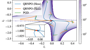
Figure 2: The trajectories of iterates $K=\mathrm{diag}(l_{1},l_{2})$ generated by QRNPO (with $\operatorname{Hess}{h}$ and $\operatorname{\text{$\overline{\operatorname{Hess}}$}}{h}$) and PGD–from different initial points–for the SLQR problem with constraint $D=\{(1,1),(2,2)\}$, over the level curves of $f$ in equation 8.

Figure 3: The trajectories of iterates $L=\left(\begin{array}[]{cc}l_{1}&l_{2}\end{array}\right)^{\intercal}$ generated by QRNPO (with $\operatorname{Hess}{h}$ and $\operatorname{\text{$\overline{\operatorname{Hess}}$}}{h}$) and PGD–from different initial points–for the OLQR problem with output matrix $C=\left(\begin{array}[]{cc}1.0&1.0\end{array}\right)$, over the level curves of $f$ in equation 8.

Next, notice that in both Figures 2 and 3, the trajectories of QRNPO with $\operatorname{Hess}$ are much more favorable in comparison to QRNPO with $\operatorname{\text{$\overline{\operatorname{Hess}}$}}$, particularly, when initialized from points further away from the local minimum and closer to the boundary. Additionally, similar to Figure 2, the region on which the unit stepsize is guaranteed to be stabilizing is relatively small in Figure 3.

Example 2 (Randomly selected system parameters).

Next, we consider an example with $n=6$ number of states and $m=3$ number of inputs, and simulate the behavior of QRNPO and PGD for 100 randomly sampled system parameters. Particularly, the parameters $(A,B)$ are sampled from a zero-mean unit-variance normal distribution, where $A$ is scaled so that the open-loop system is stable, i.e., $K_{0}=0$ is stabilizing, and the pair is controllable. Furthermore, we choose $Q=\Sigma=I_{n}$ and $R=I_{m}$ in order to consistently compare the convergence behaviors across different samples. For the SLQR problem, we randomly sample for the sparsity pattern $D$ so that at least half of the entries are zero and all of them have converged from $K_{0}=0$ in less than 30 iterations. For the OLQR problem, we also randomly sample the output matrix $C$ with $d=2$, where $98\%$ and $92\%$ of the corresponding iterates have converged from $K_{0}=0$ in less than 50 iterations using $\operatorname{Hess}$ and $\operatorname{\text{$\overline{\operatorname{Hess}}$}}$, respectively.

The minimum, maximum and median progress of the three algorithms for both SLQR and OLQR problems are illustrated in Figure 4(a) and Figure 4(b), respectively. As guaranteed by Theorem 4.3, the linear-quadratic convergence behavior of QRNPO is observed in these problems. Especially, the quadratic behavior starts as soon as the stability certificate exceeds 1. In both cases, QRNPO with $\operatorname{Hess}{h}$ (blue curves) built upon the Riemannian connection has a superior convergence rate compared with the case of using the Euclidean connection (orange curves); this was expected as the Riemannian connection is compatible with the metric induced by the geometry inherent to the cost function itself. This superior performance of QRNPO with $\operatorname{Hess}{h}$, in the meantime, requires computation of the Christoffel symbols.

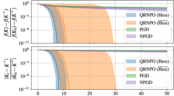
(a)

(b)

Figure 4: The min, max and median progress of normalized error of iterates and cost values at each iteration of QRNPO (with $\operatorname{Hess}{h}$ and $\operatorname{\text{$\overline{\operatorname{Hess}}$}}{h}$), PGD and NPGD for the (a) SLQR and (b) OLQR problems with 100 different randomly sampled system parameters, sparsity patterns and output matrices.

7 Conclusions and Future Directions

In this work, we considered the problem of optimizing a smooth function over submanifolds of Schur stabilizing controllers $\mathcal{S}$. In order to treat this problem in a more general setting, we studied the first and second order behavior of a smooth function when constrained to an embedded submanifold from an extrinsic point of view. Subsequently, using the second order information of the restricted function, we developed an algorithm that guarantees convergence to local minima–at least with a linear rate–and eventually with a quadratic rate. Combining this approach with backtracking line-search techniques or positive definite modifications of the Hessian operator [49, 50] can be considered as immediate future directions for a global convergence analysis.

Even though the proposed algorithm depends on the linear structure of $\widetilde{\mathcal{S}}$ , the machinery developed here can be utilized for other submanifolds, a topic that will be considered in our future works. For example, in contrast to the SLQR and OLQR problems considered, we can explore how a constraint on the average input energy translates to a nonlinear constraint that pertains to the inherent geometry of the LQR problem. In this direction, we define the average input energy, $\textstyle E_{\bm{u}}\coloneqq\mathop{\mathbb{E}}_{{\bm{x}}_{0}\sim\mathcal{D}}\|{\bm{u}}\|_{\ell_{2}}^{2},$ where $\|.\|_{\ell_{2}}$ refers to $\ell_{2}$-norm. If a static linear policy, i.e., ${\bm{u}}=K{\bm{x}}$ for $K\in\mathcal{S}$, is desired for this problem setup, then the closed-loop system assumes the form ${\bm{x}}_{k}=(A_{\mathrm{cl}})^{k}{\bm{x}}_{0}$; one can now show that under the usual identification of $T_{K}\mathcal{S}$ with ${\text{M}(m\times n,\mathbb{R})}$, we have $E_{\bm{u}}(K)=\left|K\right|_{\mathchoice{\raisebox{4.2679pt}{$\displaystyle g_{\!{}_{K}}$}}{\raisebox{4.2679pt}{$\textstyle g_{\!{}_{K}}$}}{\raisebox{4.2679pt}{$\scriptstyle g_{\!{}_{K}}$}}{\raisebox{4.2679pt}{$\scriptscriptstyle g_{\!{}_{K}}$}}}^{2}$. But then, $E_{\bm{u}}\colon\mathcal{S}\mapsto{\mathbb{R}}$ is smooth by composition, and as such, every regular level set of $E_{\bm{u}}$ translates to an upperbound on the average input energy. Regular Level Set Theorem now implies that the average input energy optimal control synthesis can be pursued via an embedded submanifold of $\mathcal{S}$ which has a nonlinear but simple structure, whenever considered in the associated Riemannian geometry. Solving this problem still requires an efficient retraction that would substitute the linear updates possible in SLQR and OLQR problems. The framework discussed in this work allows the integration of such retractions in the synthesis procedure. As such, the proposed work opens up a new approach for solving a wide range of constrained optimization problems over the manifold of Schur stabilizing controllers.

[] Shahriar Talebi (Student Member, IEEE) received the Ph.D. degree in aeronautics and astronautics, specializing in control theory, and the M.Sc. degree in Mathematics, focusing on differential geometry, both from the University of Washington, Seattle, WA, USA, in 2023. He also received the B.Sc. degree from Sharif University of Technology, Tehran, Iran, in 2014, and the M.Sc. degree from the University of Central Florida, Orlando, FL, in 2017, both in electrical engineering.

His research interests include control theory, differential geometry, learning for control, networked dynamical systems, and game theory.

Dr. Talebi was the recipient of the 2022 Excellence in Teaching Award at UW. He is also a recipient of a number of scholarships, including the William E. Boeing Endowed Fellowship, Paul A. Carlstedt Endowment, and Latvian Arctic Pilot-A. Vagners Memorial Scholarship (UW, 2018–2019), as well as the Frank Hubbard Engineering Scholarship (UCF, 2017).

[] Mehran Mesbahi (Fellow, IEEE) received his Ph.D. degree in electrical engineering-systems from University of Southern California, Los Angeles, CA, USA, in 1996.

M. Mesbahi was a member of the Guidance, Navigation, and Analysis group at JPL, Pasadena, CA, USA, from 1996–2000 and an Assistant Professor of Aerospace Engineering and Mechanics at the University of Minnesota from 2000–2002. He is currently a Professor of Aeronautics and Astronautics, Adjunct Professor of Electrical and Computer Engineering and Mathematics at the University of Washington, and the Executive Director of the Joint Center for Aerospace Technology Innovation. He was the recipient of NSF CAREER Award, NASA Space Act Award, UW Distinguished Teaching Award, UW College of Engineering Innovator Award for Teaching, and is a member of Washington State Academy of Sciences.

His research interests include distributed and networked aerospace systems, autonomy, and system and control theory.

References

- [1] H. Mohammadi, A. Zare, M. Soltanolkotabi, and M. R. Jovanović, “Convergence and sample complexity of gradient methods for the model-free linear–quadratic regulator problem,” IEEE Transactions on Automatic Control, vol. 67, no. 5, pp. 2435–2450, 2021.
- [2] M. Rotkowitz and S. Lall, “A characterization of convex problems in decentralized control∗,” IEEE Transactions on Automatic Control, vol. 51, no. 2, pp. 274–286, 2006.
- [3] J. Ackermann, “Parameter space design of robust control systems,” IEEE Transactions on Automatic Control, vol. 25, no. 6, pp. 1058–1072, 1980.
- [4] H. Feng and J. Lavaei, “On the exponential number of connected components for the feasible set of optimal decentralized control problems,” in 2019 American Control Conference (ACC), pp. 1430–1437, 2019.
- [5] W. Levine and M. Athans, “On the determination of the optimal constant output feedback gains for linear multivariable systems,” IEEE Transactions on Automatic Control, vol. 15, no. 1, pp. 44–48, 1970.
- [6] B. Anderson and J. Moore, Linear Optimal Control. Englewood Cliffs, New Jersey, Prentice–Hall, 1971.
- [7] D. Moerder and A. Calise, “Convergence of a numerical algorithm for calculating optimal output feedback gains,” IEEE Transactions on Automatic Control, vol. 30, no. 9, pp. 900–903, 1985.
- [8] H. T. Toivonen, “A globally convergent algorithm for the optimal constant output feedback problem,” International Journal of Control, vol. 41, no. 6, pp. 1589–1599, 1985.
- [9] P. Makila and H. Toivonen, “Computational methods for parametric LQ problems–a survey,” IEEE Transactions on Automatic Control, vol. 32, no. 8, pp. 658–671, 1987.
- [10] H. T. Toivonen and P. M. Makila, “Newton’s method for solving parametric linear quadratic control problems,” International Journal of Control, vol. 46, no. 3, pp. 897–911, 1987.
- [11] T. Iwasaki, R. Skelton, and J. Geromel, “Linear quadratic suboptimal control with static output feedback,” Systems & Control Letters, vol. 23, no. 6, pp. 421–430, 1994.
- [12] T. Rautert and E. W. Sachs, “Computational design of optimal output feedback controllers,” SIAM Journal on Optimization, vol. 7, no. 3, pp. 837–852, 1997.
- [13] K. Mårtensson and A. Rantzer, “Gradient methods for iterative distributed control synthesis,” in Proceedings of the IEEE Conference on Decision and Control, pp. 549–554, IEEE, 2009.
- [14] V. L. Syrmos, C. T. Abdallah, P. Dorato, and K. Grigoriadis, “Static output feedback-a survey,” Automatica, vol. 33, no. 2, pp. 125–137, 1997.
- [15] V. Blondel and J. N. Tsitsiklis, “NP-hardness of some linear control design problems,” SIAM journal on control and optimization, vol. 35, no. 6, pp. 2118–2127, 1997.
- [16] C. H. Papadimitriou and J. Tsitsiklis, “Intractable problems in control theory,” SIAM Journal on Control and Optimization, vol. 24, no. 4, pp. 639–654, 1986.
- [17] J. Bu, A. Mesbahi, M. Fazel, and M. Mesbahi, “LQR through the lens of first order methods: Discrete-time case,” arXiv preprint arXiv:1907.08921, 2019.
- [18] J. Bu, A. Mesbahi, and M. Mesbahi, “Policy gradient-based algorithms for continuous-time linear quadratic control,” arXiv preprint arXiv:2006.09178, 2020.
- [19] M. Fazel, R. Ge, S. Kakade, and M. Mesbahi, “Global convergence of policy gradient methods for the linear quadratic regulator,” in Proceedings of the 35th International Conference on Machine Learning, vol. 80, pp. 1467–1476, PMLR, 10–15 Jul 2018.
- [20] I. Fatkhullin and B. Polyak, “Optimizing static linear feedback: Gradient method,” SIAM Journal on Control and Optimization, vol. 59, no. 5, pp. 3887–3911, 2021.
- [21] H. Mohammadi, M. Soltanolkotabi, and M. R. Jovanovic, “On the linear convergence of random search for discrete-time LQR,” IEEE Control Systems Letters, vol. 5, no. 3, pp. 989–994, 2021.
- [22] F. Zhao, K. You, and T. Başar, “Global convergence of policy gradient primal–dual methods for risk-constrained LQRs,” IEEE Transactions on Automatic Control, vol. 68, no. 5, pp. 2934–2949, 2023.
- [23] Y. Park, R. Rossi, Z. Wen, G. Wu, and H. Zhao, “Structured policy iteration for linear quadratic regulator,” in International Conference on Machine Learning, pp. 7521–7531, PMLR, 2020.
- [24] D. Gabay, “Minimizing a differentiable function over a differential manifold,” Journal of Optimization Theory and Applications, vol. 37, no. 2, pp. 177–219, 1982.
- [25] S. T. Smith, “Optimization techniques on Riemannian manifolds,” Fields Institute Communications, vol. 3, no. 3, pp. 113–135, 1994.
- [26] P.-A. Absil, R. Mahony, and R. Sepulchre, Optimization Algorithms on Matrix Manifolds. Princeton University Press, 2009.
- [27] S.-I. Amari, “Natural gradient works efficiently in learning,” Neural Computation, vol. 10, no. 2, pp. 251–276, 1998.
- [28] S.-I. Amari and S. Douglas, “Why natural gradient?,” in Proceedings of the IEEE International Conference on Acoustics, Speech and Signal Processing (ICASSP), vol. 2, pp. 1213–1216 vol.2, 1998.
- [29] J. M. Lee, Introduction to Riemannian Manifolds. Cham, Switzerland: Springer Nature, 2nd ed., 2018.
- [30] S. Talebi and M. Mesbahi, “Riemannian constrained policy optimization via geometric stability certificates,” in 2022 IEEE 61st Conference on Decision and Control (CDC), pp. 1472–1478, 2022.
- [31] Z. Gajic and M. T. J. Qureshi, Lyapunov Matrix Equation in System Stability and Control. Courier Corporation, 2008.
- [32] J. M. Lee, Introduction to Smooth Manifolds. Springer, 2nd ed., 2013.
- [33] S. Skogestad and I. Postlethwaite, Multivariable Feedback Control: Analysis and design. Hoboken, NJ, USA: Wiley-Blackwell, 2nd ed., 2005.
- [34] M. Mesbahi and M. Egerstedt, Graph Theoretic Methods in Multiagent Networks. Princeton University Press, 2010.
- [35] J. Bu, A. Mesbahi, and M. Mesbahi, “On topological and metrical properties of stabilizing feedback gains: the MIMO case,” arXiv preprint arXiv:1904.02737, 2019.
- [36] D. Serre, Matrices: Theory and Applications. Springer Science and Media, 2nd ed., 2010.
- [37] J. Lee, Introduction to Topological Manifolds. Springer Science & Business Media, 2nd ed., 2010.
- [38] A. Ohara and S.-I. Amari, “Differential geometric structures of stable state feedback systems with dual connections,” IFAC Proceedings, vol. 25, no. 21, pp. 176–179, 1992.
- [39] P. A. Absil, R. Sepulchre, P. Van Dooren, and R. Mahony, “Cubically convergent iterations for invariant subspace computation,” SIAM Journal on Matrix Analysis and App., vol. 26, no. 1, pp. 70–96, 2004.
- [40] J. Müller and G. Montúfar, “Geometry and convergence of natural policy gradient methods,” Information Geometry, pp. 1–39, 2023.
- [41] F. Alvarez, J. Bolte, and O. Brahic, “Hessian Riemannian gradient flows in convex programming,” SIAM Journal on Control and Optimization, vol. 43, no. 2, pp. 477–501, 2004.
- [42] G. Hewer, “An iterative technique for the computation of the steady state gains for the discrete optimal regulator,” IEEE Transactions on Automatic Control, vol. 16, no. 4, pp. 382–384, 1971.
- [43] J. P. Hespanha, Linear Systems Theory. Princeton Univ. Press, 2018.
- [44] G. C. Goodwin, S. F. Graebe, and M. E. Salgado, Control System Design. Upper Saddle River, NJ: Prentice Hall, 2001.
- [45] K. Mårtensson, Gradient Methods for Large-Scale and Distributed Linear Quadratic Control. PhD thesis, Lund University, 2012.
- [46] S. Talebi, S. Alemzadeh, N. Rahimi, and M. Mesbahi, “On regularizability and its application to online control of unstable LTI systems,” IEEE Transactions on Automatic Control, vol. 67, no. 12, pp. 6413–6428, 2022.
- [47] S. Talebi and M. Mesbahi, “Policy optimization over submanifolds for constrained feedback synthesis,” arXiv preprint arXiv:2201.11157, 2022.
- [48] S. Talebi and M. Mesbahi, “Quasi Riemannian Newton Policy Optimization (QRNPO),” 2022. Available on GitHub at https://github.com/shahriarta/QRNPO.
- [49] J. E. Dennis Jr and R. B. Schnabel, Numerical Methods for Unconstrained Optimization and Nonlinear Equations. Society for Industrial and Applied Mathematics, 1996.
- [50] J. Nocedal and S. Wright, Numerical Optimization. Springer Science & Business Media, 2006.
- [51] S. G. Krantz and H. R. Parks, A Primer of Real Analytic Functions. Springer Science & Business Media, 2002.
- [52] J. Milnor, Morse Theory, vol. 51. Princeton University Press, 1963.
[![[Uncaptioned image]](/html/2201.11157/assets/images/shahriar.jpg) ]