Nonlinear quantum interferometric spectroscopy with entangled photon pairs

Abstract

We develop closed expressions for a time-resolved photon counting signal induced by an entangled photon pair in an interferometric spectroscopy setup. Superoperator expressions in Liouville-space are derived that can account for relaxation and dephasing induced by coupling to a bath. Interferometric setups mix matter and light variables non-trivially, which complicates their interpretation. We provide an intuitive modular framework for this setup that simplifies its description. Based on separation between the detection stage and the light-matter interaction processes. We show that the pair entanglement time and the interferometric time-variables control the observed physics time-scale. Only a few processes contribute in the limiting case of small entanglement time with respect to the sample response, and specific contributions can be singled out.

I Introduction

Interferometric setups introduce a promising new methodology for quantum inference of matter information in quantum spectroscopy [1, 2, 3, 4, 5]. Since quantum probes change their state upon interaction with external systems, multiphoton coincidence detection schemes should reveal quantum correlations induced by the sample [6, 7]. We consider the optical measurement setup shown in Fig. 1 – that includes linear and nonlinear elements that transform the optical field before and after it is coupled to a sample. We focus on time-resolved detection of two photons. We use one interferometric setup to prepare the initial quantum state of the light, followed by a second interferometer that manipulates the arrival times of matter induced radiation to obtain matter pathway resolution. Interferometric schemes such as the Mach-Zehnder [8], Hong-Ou-Mandel [9], and Franson [10] provide a useful toolbox to scan the change in photon statistics by coupling to a sample from which matter information may be inferred using multiphoton detection in coincidence [11, 10, 12]. Quantum-enhancements of interferometric detection schemes are an experimental reality in several fields [13]. The direct detection of gravitational waves [14, 15, 16], unprecedented phase estimation precision with high loss tolerance at lower photon flux [17, 18, 19, 20, 21], and in wide-field imaging [22] are all contemporary examples. Here, we introduce a new family of signals applied to the inference of objects at the microscopic scale.

Liouville-space pathways break-down the density operator evolution into the set of physical processes determined by time ordered excitation and de-excitation processes (pathways) induced by the applied fields. Sorting them out is important in order to develop understanding the underlying matter dynamics. This description become crucially important when considering the effects of the environment that break time reversal symmetry. Sorting these pathways allows to infer the role of each process in a systematic manner. Liouville pathway resolution enable to compare model-based theoretical predictions with experiment [23].

Our goal is to sort out the Liouville-space pathways, by scanning interferometric delays in the preparation and detection stages. We wish to identify what type of information regarding the dynamics of the system and its coupling to a bath can be inferred from these measurements. We consider two interferometers, at the preparation and detection processes, as depicted in Fig. 1 and further discussed in Sec. II. Two-port linear interferometers induce transformations in the two-photon space [24, 25]. They generate rotations in the basis of the electromagnetic field [1]. These transformations offer a unique set of control knobs used in both the preparation and detection stages. These control parameters provide novel spectral windows [2]. We show that the interferometric control variables enable to conveniently scan the temporal dynamics. We derive compact superoperator expressions for the time-resolved coincidence-signal of two photons expanded in terms of Liouville-space pathways. For simplicity, we consider two ideal detectors which is fast in comparison to all relaxation times of the sample. This extends Glauber’s celebrated theory of detection [26].

The general expressions are given in appendix B. For simplicity we have derived an approximation for the limiting case of vanishing two-photon temporal separation (the entanglement time $T_{e}$). The two photons then arrive simultaneously relative to the observed dynamics timescale. This corresponds to a vanishing moving time average of the response, thus sensitive to the dynamics above $T_{e}$ which is in the femtosecond regime. At this time scales we expect environment effects to be more pronounced which requires the Liouville space approach. Moreover, using the novel time variables, we are able to separate different processes in the evolution of the sample in time domain, from which different transport mechanisms can be studied in detail such as exciton-exciton scattering [27, 28, 29].

II The setup

Our setup shown in Fig. 1a contains two interferometers. An entangled pair is prepared using a Michelson interferometer as introduced in [13, 30, 31] and depicted in Fig. 1b. At the detection stage we employ a Hong-Ou-Mandel interferometer. In this section we provide the theoretical framework required for the inclusion of both interferometers.

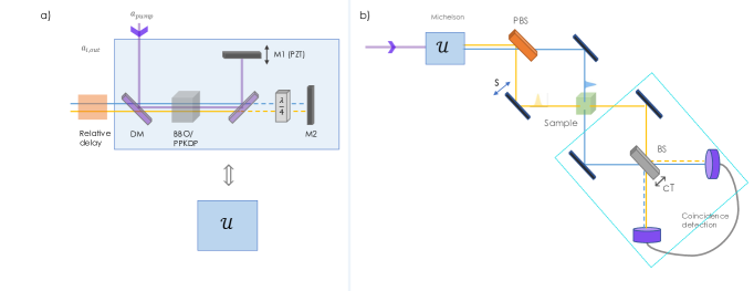
Figure 1: The quantum interferometry setup.(a) The Michelson interferometer ${\cal U}$ generates a pair of photons with variable exchange-phase $\theta$, used as a control for the photon-pair degree of distinguishability (see Eq. 2). The photons acquire the relative delay $s$. (b) State preparation protocol in which two photons are generated with a possible relative delay, then coupled to thee sample and finally detected in coincidence in a Hong-Ou-Mandel interferometer (boxed area).

Each stage in the setup, introduces a superposition of fields which we denote basis rotation or transformation. These platforms are presented in a modular manner such that each stage is responsible for a well defined property (e.g., introducing a delay). Quantum mechanically, the stages are inseparable since more than one absorption, emission and detection events occur in all possible time orderings. However, we limit the discussion to a distant detection plane, such that the propagation time of the emitted photons is much longer than the typical time of the entire process. The detection and interaction are then completely factorized temporally as depicted in Fig. 2

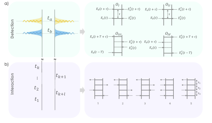
Figure 2: Block design for two-photon interferometric spectroscopy. Decoupling of the interaction and detection process when both are well temporally defined. (a) The detection pathways corresponding to HOM interferometer placed after the sample. Here $\tau>0$ is the detection time difference of the two photons and $T>0$ is the HOM delay. Two paths of direct propagation $O_{I-II}$, along with $O_{III-IV}$ in which there is a coherence between reflected and transmitted modes. (b) Ladder diagrams that correspond to the light-matter interaction corresponding to the matter correlation functions in Eq. 8a (for a three-level model system). Only processes in which two-photons interact with the sample and two are detected and sketched.

II.1 Interferometric state preparation

We assume a broadband ultrafast pump pulse which is known to imprint identifying spectral information on each of the optical modes. The modified Michelson interferometer in Fig. 1a, generates control over this feature by controlled systematization of the wavefunction in a type-II phase matching setting. This results in engineered degree of distinguishability as discussed below.

The pump beam is reflected by the dichroic mirror (DM) then passes the first time through the BBO crystal. The generated entangled pair passes through the $\nicefrac{{\lambda}}{{4}}$ plate that switches the polarization such that $\phi\left(\omega_{a},\omega_{b}\right)\rightarrow\phi\left(\omega_{b},\omega_{a}\right)$, then exits the interferometer from the left. Otherwise, the pump photon is reflected by the second DM and passes through the BBO crystal for the second time with a controlled phase introduced by the PZT device on which mirror M1 is positioned generating possibly an entangled pair. Finally the pump beam is filtered out of the interferometer by the first DM.

The combined nonlinear interferometer transformations create a two photon wavefunction of the form

$$|\Psi_{\theta}\rangle=\int d\omega_{a}d\omega_{b}\Phi_{\theta}\left(\omega_{a},\omega_{b}\right)a^{\dagger}\left(\omega_{a}\right)b^{\dagger}\left(\omega_{b}\right)|\text{vac}\rangle.$$ (1)

The amplitude is given by

$$\Phi_{\theta}\left(\omega_{a},\omega_{b}\right)=\frac{1}{\sqrt{2}}\left[\phi\left(\omega_{a},\omega_{b}\right)+e^{i\theta}\phi\left(\omega_{b},\omega_{a}\right)\right].$$ (2)

The joint spectral amplitude (JSA) resulting from the direct-channel $\phi\left(\omega_{a},\omega_{b}\right)$ (due to one pass in the BBO with aligned polarizations) used in our calculations is given by $\phi\left(\omega_{a},\omega_{b}\right)={\cal A}_{p}\left(\omega_{a}+\omega_{b}\right)\varphi\left(\omega_{a},\omega_{b}\right)$. The Gaussian pump envelope ${\cal A}_{p}\left(\omega\right)=\exp\left[\nicefrac{{\left(\omega-\omega_{p}\right)^{2}}}{{\sigma_{p}^{2}}}\right]$ is centered around $\omega_{p}$ characterized with the bandwidth $\sigma_{p}$ [32]. The phase-matching factor $\varphi\left(\omega_{a},\omega_{b}\right)=\text{sinc}\left[\left(\omega_{a}-\bar{\omega}_{a}\right)T_{a}+\left(\omega_{b}-\bar{\omega}_{b}\right)T_{b}\right]$, breaks the frequency exchange symmetry, i.e., $\varphi\left(\omega_{a},\omega_{b}\right)\neq\varphi\left(\omega_{b},\omega_{a}\right)$. Here $\bar{\omega}_{a/b}$ is the central frequency of the signal and idler beams, and $T_{a/b}=L\left(v_{a/b}^{-1}-v_{p}^{-1}\right)$, where $L$ is the nonlinear crystal length and $v$ is the inverse group velocity at the relevant central frequency $\left(\bar{\omega}_{a/b},\omega_{p}\right)$. In this (type-II) phase matching condition, the channels are flipped using the their opposite and orthogonal polarization degree of freedom, e.g., $|\Psi_{\theta}\rangle=|HV\rangle+e^{i\theta}|VH\rangle$ where $V$ and $H$ correspond to horizontal and vertical polarizations respectively. For different phase matching condition which give rise to identiclly polarized biphotons, one would expect a different output, e.g., $|\Psi_{\theta}\rangle=|HH\rangle+e^{i\theta}|VV\rangle$.

Here, we have calculated the preparation step in the Schödinger picture, modifying the initial amplitude rather than the fields operators. The detection stage is computed using the Heisenberg picture as explained in Sec. III. This way, the dynamics is calculated in the matter’s reference-frame, as done in [2]. Each interferometer introduces additional spectroscopic control parameters that can be used to study the joint light-matter quantum state.

III Detection pathways

The detection process involves a HOM interferometer as shown in the boxed area of Fig. 1b. We define the signal in time domain. We consider a sample described by the Hamiltonian $H_{\mu}$, that is coupled to field degrees of freedom $H_{\phi}$ by the dipolar interaction $H_{\text{int}}=\boldsymbol{\mu}\left(\boldsymbol{r},t\right)\cdot\boldsymbol{E}\left(\boldsymbol{r},t\right)$. Here $\boldsymbol{\mu}\left(\boldsymbol{r},t\right)=\boldsymbol{V}\left(\boldsymbol{r},t\right)+\boldsymbol{V}^{\dagger}\left(\boldsymbol{r},t\right)$ is the dipole operator, $\boldsymbol{V}=\sum_{i<j}\mu_{ij}|i\rangle\langle j|$ is a lowering transition operator acting in the molecular Hilbert space with the corresponding matrix element $\mu_{ij}$, $\boldsymbol{E}\left(\boldsymbol{r},t\right)=\sum_{\sigma}\left[E_{\sigma}\left(\boldsymbol{r},t\right)+\text{H.c. }\right]$ is the electric field operator given by $E_{\sigma}\left(\boldsymbol{r},t\right)=\sum_{\boldsymbol{k}}\sqrt{\frac{2\pi k}{\Omega_{Q}}}\hat{\epsilon}_{\sigma}\left(\boldsymbol{k}\right)a_{\boldsymbol{k},\sigma}\left(t\right)e^{i\boldsymbol{k}\cdot\boldsymbol{r}}$, where $\hat{\epsilon}_{\sigma}\left(\boldsymbol{k}\right)$ is the $\sigma$-polarization vector, $\Omega_{Q}$ is the quantization volume ($c=1$), and $a_{\boldsymbol{k},\sigma}\left(a_{\boldsymbol{k},\sigma}^{\dagger}\right)$ are (bosonic) photon annihilation (creation) operators obeying $\left[a_{\boldsymbol{k},\sigma},a_{\boldsymbol{k}^{\prime},\sigma^{\prime}}^{\dagger}\right]=\delta_{\sigma,\sigma^{\prime}}\delta_{\boldsymbol{k},\boldsymbol{k}^{\prime}}$. Hereafter we assume that the applied field is near resonance with a molecular transition, such that the rotating wave approximation may be applied by setting $H_{\text{int}}=EV^{\dagger}+E^{\dagger}V$.

The two-photon coincidence signal is defined by

$$\hat{{\cal O}}\left(t,\tau\right) =E_{a^{\prime},R}^{\dagger}\left(\boldsymbol{r}_{a},t\right)E_{b^{\prime},R}^{\dagger}\left(\boldsymbol{r}_{b},t+\tau\right)$$ (3)

$$\times E_{b^{\prime},L}\left(\boldsymbol{r}_{b},t+\tau\right)E_{a^{\prime},L}\left(\boldsymbol{r}_{a},t\right).$$

Here, $E_{R}$ and $E_{L}$ are electric field superoperators that act from the right $E_{R}\rho\equiv\rho E$, and left $E_{L}\rho\equiv E\rho$ of the density operator. We further define their linear combinations $A_{\pm}O=A_{L}O\pm A_{R}O$ (corresponding to Hilbert-space commutator and anti commutator). These will be useful for the compact description in the interaction picture below. The primes reflect the fact that the detection and interaction planes are described in different basis sets due to the HOM transformation, as explained below.

III.1 The HOM detection interferometer

In our setup in Fig. 1, two beams are combined on a beam splitter (BS) which is mounted on a movable stage. This enables to scan variable propagation times of the reflected pathways of the beam with respect to the transmitted ones, introducing the HOM time-delay $T$. This process is described by a linear transformation since the photons at the detection plane are represented in a different basis. The transformation (Jordan-Schwinger map) can be represented as an $SU\left(2\right)$ rotation in the frequency-domain [33, 34, 24, 35, 25], resulting in the input-output relation for the field operators. Writing the field in vector notation given by $\boldsymbol{E}\left(\boldsymbol{r},\omega\right)=\left(E_{a}\left(\boldsymbol{r},\omega\right),E_{b}\left(\boldsymbol{r},\omega\right)\right)^{T}$, the HOM rotation the detected field is given by $\boldsymbol{E}|_{\text{detection}}\left(\boldsymbol{r},\omega\right)=\hat{{\cal R}}_{T}\boldsymbol{E}|_{\text{interaction}}\left(\boldsymbol{r},\omega\right)$ where $\hat{{\cal R}}_{T}$ is given by

$$\hat{{\cal R}}_{T}=\left(\begin{array}[]{cc}t&ire^{i\omega T}\\ ire^{-i\omega T}&t\end{array}\right).$$ (4)

Here $t$ and $r$ are the transmission and reflection coefficients obeying $\left|t\right|^{2}+\left|r\right|^{2}=1$. For the 50:50 BS considered here, $t=r=\nicefrac{{1}}{{\sqrt{2}}}$. In the following, we express all field operators in the matter interaction-domain basis $\boldsymbol{E}|_{\text{interaction}}\equiv\boldsymbol{E}\left(\boldsymbol{r},\omega\right)$, which requires the inverse rotation of the observable in Eq. 3 [1].

III.2 The observable

Glauber’s $G^{\left(2\right)}$$\left(\tau\right)$ coincidence signal is formally given by the expectation value of this observable, evolved using the total density matrix of the field and matter in the interaction picture

$${\cal C}\left(t,\tau\right) =\left\langle{\cal T}\hat{{\cal O}}^{\prime}\left(t,\tau\right)e^{-\frac{i}{\hbar}\underset{-\infty}{\overset{t^{*}}{\int}}dsH{}_{\text{int},-}\left(s\right)}\right\rangle,$$ (5)

here ${\cal T}$ is the time ordering superoperator that maintains the bookkeeping of the interaction events, e.g., ${\cal T}A\left(t_{1}\right)B\left(t_{2}\right)=\theta\left(t_{1}-t_{2}\right)A\left(t_{1}\right)B\left(t_{2}\right)+\theta\left(t_{2}-t_{1}\right)B\left(t_{2}\right)A\left(t_{1}\right)$, the Heaviside step-function is defined by $\theta\left(t\right)=1,$ $\forall t\geq 0$ and $\theta\left(t\right)=0$, $\forall t<0$. Note that the interaction Hamiltonian superoperator is represented by the field modes prior to the transformation. HOMI introduces the time delay $T$ as an additional control parameter to the observable superoperator $O\left(t,\tau\right)\rightarrow O\left(t,\tau,T\right)$. For the HOM detection setup, we should transform the observable in Eq. 3 according to the HOM transformation (Eq. 4), resulting in 16 detection pathways. Only the four – in which one photon of each mode are detected – contribute to our signal (see also [9]), reducing Eq. 3 to

$$\hat{{\cal O}}^{\prime}\left(t,\tau,T\right) =O_{I}+O_{II}+O_{III}+O_{IV}$$ (6)

where the detection pathways are given by

$$O_{I} =E_{a,R}^{\dagger}\left(\boldsymbol{r}_{a},t\right)E_{b,R}^{\dagger}\left(\boldsymbol{r}_{b},t+\tau\right)E_{b,L}\left(\boldsymbol{r}_{b},t+\tau\right)E_{a,L}\left(\boldsymbol{r}_{a},t\right)$$ (7a)

$$O_{II} =E_{b,R}^{\dagger}\left(\boldsymbol{r}_{a},t\right)E_{a,R}^{\dagger}\left(\boldsymbol{r}_{b},t+\tau\right)E_{a,L}\left(\boldsymbol{r}_{b},t+\tau\right)E_{b,L}\left(\boldsymbol{r}_{a},t\right)$$ (7b)

$$O_{III} =-E_{a,R}^{\dagger}\left(\boldsymbol{r}_{a},t\right)E_{b,R}^{\dagger}\left(\boldsymbol{r}_{b},t+\tau\right)$$ (7c)

$$\times E_{a,L}\left(\boldsymbol{r}_{b},t+T+\tau\right)E_{b,L}\left(\boldsymbol{r}_{a},t-T\right)$$

$$O_{IV} =-E_{b,R}^{\dagger}\left(\boldsymbol{r}_{a},t-T\right)E_{a,R}^{\dagger}\left(\boldsymbol{r}_{b},t+T+\tau\right)$$ (7d)

$$\times E_{b,L}\left(\boldsymbol{r}_{b},t+\tau\right)E_{a,L}\left(\boldsymbol{r}_{a},t\right).$$

Note that since Eq. 6 is given in the basis of the interaction domain (different from Eq. 3), none of the quantities are primed in the definition of $\hat{{\cal O}}$ as well as the field operators $E_{m,X}$ ($m\in\left\{a,b\right\}$; $X\in\left\{L,R\right\}$). We have explicitly included the HOM delay $T$ variable to the coincidence observable, which is expressed in $O_{III-IV}$ and a $\left(-\right)$ sign [Eq. 6]. All four combinations depicted in Fig. 2a (top-right) contribute to the interferometric coincidence signal. When the BS is removed, the ordinary coincidence detection setup can also be recovered by only keeping the $O_{I}$ contributions.

IV The interaction pathways

We expand the signal in Eq. 5 pertubatively to $4^{\text{th}}$ order in $H_{\text{int}}$ such that each photon interacts twice with the sample. Generally, 4 interactions generate 16 left-right Liouville pathways. In addition, each arrow may point inward/outward resulting in a total of 256 possible pathways. As depicted in Figs. 2a and b, this number is significantly reduced mainly due to the coincidence detection and the initial Fock state. Note that Fig. 2b contains half of the contributions and their complex conjugates should be added. It is possible to further reduce the number of contributions, by the following considerations. Near resonance, the rotating wave approximation (RWA) can be invoked, resulting in the simplified interaction Hamiltonian $H_{\text{int}}=EV^{\dagger}+E^{\dagger}V$. We further consider the three level model systems depicted in Fig. 3, initially in the ground state $\rho_{0}=|g\rangle\langle g|$, so that the first interaction can only be excitation (no de-excitation). This eliminates contributions in which an emission event occurs after a single photon is detected. The expectation value $\left\langle\hat{{\cal O}}\right\rangle$ is and expectation value and thus real (note that the diagrams in Fig. 3 are symmetric with respect to exchange of L-R and taking the complex conjugate). By convention, we only include pathways in which the last interaction is taken from the left side with an outgoing arrow (generated a detected photon). The contributions in which the last interaction is from the right are related to these by conjugation and interchanging L-R. The full signal is finally given by $2\mathfrak{Re}\left\langle\hat{{\cal O}}p_{i}\right\rangle$ where $p_{i}$ denotes all pathways terminated at the left. The top interaction from the left must point outwards, otherwise this mode is not occupied, hence not detected. Photon number conservation implies equal number of inward/outward arrows. Only diagrams in which two photons interact with the sample and two photons are detected contribute to the signal. Since two-photon population is detected, diagrams in which there is a single arrow in one of the sides are eliminated.

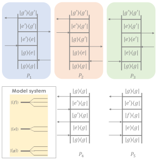
Figure 3: Interaction pathways for three-level exciton model. The five interaction pathways with the respective exciton dynamics for the selected three-level exciton model system. Each energy manifold $|\left\{\boldsymbol{g}\right\}\rangle,|\left\{\boldsymbol{e}\right\}\rangle,|\left\{\boldsymbol{f}\right\}\rangle$ is composed of several states.

The five surviving pathways are depicted in Fig. 3, all contain two field modes from each side of the density operator. Their complex conjugates should be added as well. These processes are labeled $P_{i}$ where $i\in\left[1,5\right]$ in Fig. 3, correspond to the superoperator correlation functions denoted ${\cal F}_{i}$ given by

$${\cal F}_{1}\left(\tau_{1},\tau_{2},\tau_{3}\right) =\left\langle V_{L}{\cal G}\left(\tau_{1}\right)V_{R}^{\dagger}{\cal G}\left(\tau_{2}\right)V_{L}^{\dagger}{\cal G}\left(\tau_{3}\right)V_{R}\right\rangle$$ (8a)

$${\cal F}_{2}\left(\tau_{1},\tau_{2},\tau_{3}\right) =\left\langle V_{L}{\cal G}\left(\tau_{1}\right)V_{L}^{\dagger}{\cal G}\left(\tau_{2}\right)V_{R}^{\dagger}{\cal G}\left(\tau_{3}\right)V_{R}\right\rangle$$ (8b)

$${\cal F}_{3}\left(\tau_{1},\tau_{2},\tau_{3}\right) =\left\langle V_{L}{\cal G}\left(\tau_{1}\right)V_{R}^{\dagger}{\cal G}\left(\tau_{2}\right)V_{R}{\cal G}\left(\tau_{3}\right)V_{L}^{\dagger}\right\rangle$$ (8c)

$${\cal F}_{4}\left(\tau_{1},\tau_{2},\tau_{3}\right) =\left\langle V_{L}{\cal G}\left(\tau_{1}\right)V_{L}^{\dagger}{\cal G}\left(\tau_{2}\right)V_{L}{\cal G}\left(\tau_{3}\right)V_{L}^{\dagger}\right\rangle$$ (8d)

$${\cal F}_{5}\left(\tau_{1},\tau_{2},\tau_{3}\right) =\left\langle V_{L}{\cal G}\left(\tau_{1}\right)V_{L}{\cal G}\left(\tau_{2}\right)V_{L}^{\dagger}{\cal G}\left(\tau_{3}\right)V_{L}^{\dagger}\right\rangle,$$ (8e)

(plus their complex conjugates). Here $\left\langle\cdots\right\rangle\equiv\text{tr}\left\{\cdots\rho_{\mu}\left(-\infty\right)\right\}$ where $\rho_{\mu}\left(-\infty\right)$ is the initial state of the matter, and Liouville-space Green’s function is given by ${\cal G}\left(t\right)=-\frac{i}{\hbar}\theta\left(t\right)e^{-i{\cal L}_{\mu}t-\eta t}$.

The matter correlation functions ${\cal F}_{j}(\tau_{1},\tau_{2},\tau_{3})$, with $j=1,\ldots,5$, presented in Eq. 8a and illustrated in Fig. 3, provide a useful microscopic insight into the capabilities of the entangled-photon spectroscopy to retrieve detailed information on ultrafast photoinduced dynamics of various chemical systems, inter alia molecular aggregates, whose dynamics is determined by the electronic interactions induced Frenkel exciton scattering and exciton-phonon interactions. Since the actual measured correlated signals are represented by convolutions of ${\cal F}_{j}$ with the doorway and window functions, the latter containing relevant information on the entangled photon sources, as well as interferometric supplement, and having nothing to do with the dynamics of the system under study, one should in first place understand what kind of a matter dynamical information is contained in the aforementioned four-point correlators.

Since all matter dynamical information, available via coherent four-wave mixing spectroscopy is fully contained in the third-order nonlinear response function

$${\cal F}_{\rm coh}=\left\langle\hat{V}_{+}{\cal G}(\tau_{1})\hat{V}_{-}{\cal G}(\tau_{2})\hat{V}_{-}{\cal G}(\tau_{3})\hat{V}_{-}\right\rangle,$$ (9)

with $\hat{V}=V+V^{\dagger}$, the differences in the spectroscopic information, provided by entangled-photon versus four-wave mixing spectroscopies, originates just from the different Liouville-space structure of the four-point matter correlators ${\cal F}$. Although the latter is apparently very different for ${\cal F}$, presented in Eq. 8a versus Eq. 9, the issue allows for a clear, simple, and conceptually explicit analysis, as follows.

Indeed, as shown, using Liouville space Green functions techniques [36, 37] and further by means of the Nonlinear Exciton Equations (NEE) [38], in the case of weak to moderate exciton-phonon coupling, when the dynamics is dominated by excitonic effects, and effects of polaron formation/self-trapping are not substantial, there are three phenomena that contribute to optical response: (i) exciton-exciton scattering, described in terms of the exciton-exciton scattering matrix $\bar{\Gamma}(\omega)$, (ii) exciton-photon coupling mediated transport, described by the exciton transport correlation function $G^{(2)}(\omega)$, and combined effects, expressed in terms of a convolutions of the two above; of course, the expressions for the response contain the one-exciton Green function $G(\omega)$ that contains of the exciton-phonon coupling induced exciton dephasing.

The Green function approach can be extended to analyze the Liouville space correlators ${\cal F}_{j}$ in Eq. (8); this analysis will be addressed in detail in a separate publication, here we just present its main outcome, to relate it to the Feynman diagrams (Fig. 3). Despite a very different Liouville-space structure of the correlators in the entangled photon versus four-wave mixing case, due to the specific features of the Frenkel exciton model with moderate exciton-photon coupling, the ingredients that enter the final expressions, namely $\bar{\Gamma}(\omega)$, $G^{(2)}(\omega)$, and $G(\omega)$ stay the same, just the final expressions get modified. Translating the results, presented in Eq. 8a from the Sum-over-States (SOS) to the exciton-scattering language, we can combine the Feynman diagrams (4) and (5) in Fig. 3 to obtain type (i) effects, i.e., pure exciton-excitons scattering; it is well known that combining these two diagrams we take care of the so-called cancellation of the $N^{2}$ terms problem, which in the exciton-scattering approach happens automatically. Combining the diagrams (1), (2), and (3) we obtain a type (ii) contribution that reflects exciton transport effects, since in diagrams (1) and (3) the system is in the population/exciton-exciton coherence state during the $\tau_{2}$ time segment. In diagram 2 the system is in the $|g\rangle\langle g^{\prime}|$, which means in the ground electronic state with a different phonon structures, it plays a proper cancellation role for exciton transport, in the way how the diagram (4) operates for exciton scattering. Note that both diagrams (2) and (4) also describe slight modifiication/renormalization of the excitons scattering matrix due to exciton-phonon coupling.

Very importantly type (iii) effects (combined exciton-exciton scattering and exciton transport) in the four-wave mixing, on the SOS language originate from the diagrams, when the system is in the population/exciton-exciton coherence and two-exciton ground state coherence ($|f\rangle\langle g|$ or $|g\rangle\langle f|$) during the time periods $\tau_{2}$ and $\tau_{3}$, respectively. Since such diagrams never appear in the entangled-photon spectroscopy case, type (iii) effects do not contribute to the signals in the latter case.

Summarizing, unlike the coherent four-wave mixing spectroscopy, the entangled-photon spectroscopy studies only effects of exciton-exciton scattering and exciton transport, with no combined contributions, thus provided a better separation of dynamical phenomena that contribute to spectroscopic data.

IV.1 The signal

In Fig. 1a we consider the HOMI detection setup. The preparation alters the primary source, resulting in the JSA given in Eq. 2. The HOMI detection transforms the $G^{\left(2\right)}\left(\tau\right)$ signal in Eq. 3 into Eq. 6.

The total signal involves summing over all the product combinations of detection pathways in Fig. 2 a with all the interaction pathways depicted in Fig. 2b (see appendix B for the expressions of all combinations for a general preparation process). The signal contains many terms corresponding to all combinations of Liouville pathways $i\in\left[1,5\right]$, with all detection pathways defined in Eq. 6 $O_{\nu}$, where $\nu=I,...,IV$. One way to think about it is that each process $P_{i}$ is obtained by a coherent superposition of all HOM detection pathways ${\cal S}_{\nu,i}$, and the signal is given by their superposition. For an illustrative example of the derivation of an contribution, see appendix B. The coincidence signal in Eq. 10 is finally given by

$${\cal C}\left(\tau,T,s\right) =2\mathfrak{Re}\left\{\sum_{\nu,i}{\cal S}_{\nu,i}\right\},$$ (10)

where ${\cal S}_{\nu,i}\equiv\text{tr}\left\{O_{\nu}P_{i}\rho\left(-\infty\right)\right\}$ and the detection and interaction pathways are labeled in Fig. 2. The detection pathways are given in Eq. 6 (see appendices for detailed expressions). Note that the density matrix is given by a product of the matter and field respectively $\rho\left(-\infty\right)\equiv\rho_{\mu}\otimes\rho_{\varphi}$. The field is traced with respect to $\rho_{\varphi}\equiv|\Psi_{\theta}\rangle\langle\Psi_{\theta}|$ using $\Phi_{\theta}\left(t_{1},t_{2}\right)=\frac{1}{\sqrt{2}}\left[\phi\left(t_{1},t_{2}\right)+e^{-i\theta}\phi\left(t_{2},t_{1}\right)\right]$ with respect to Eq. 1 due to the Michelson interferometer.

The short entanglement-time limit

We no invoke an approximation which greatly simplifies this signal. Consider a symmetric joint spectral amplitude, obtained by either using $\theta=0$ in Eq. 2, or via a narrowband pump. In either case, the entanglement time $T_{e}$ represents the time window in which both photons arrive [30]. We also consider the characteristic timescale for the matter dynamics to be bound from above by $\tau_{\text{R}}$. We focus on the regime $\tau_{R}\gg T_{e}$ such that both photons arrive simultaneously. The relative delay $s$ introduced in Fig. 1a between the pair, now sets the time interval in which all interactions occur. In this limit, the amplitude is approximated by a narrow distribution

$$\Phi\left(t_{1},t_{2}\right)\rightarrow\delta\left(t_{1}-t_{2}-s\right).$$ (11)

Consequently, processes with vanishing time intervals between interactions do not contribute to this order $\left(\tau_{1},\tau_{2},\tau_{3}\right)\neq 0$. Note that $\Phi\left(t_{1},t_{2}\right)$ is symmetric to $t_{1}\leftrightarrow t_{2}$ exchange under this approximation which is consistent with $\theta=0$. Here the Michelson interferometer is used for rectification of the exchange phase $\theta$ when an ultrafast pump is used. Alternatively, a narrowband pump can be used in which the exchange phase correction is no longer essential. Since $\left(T,\tau,s\right)$ are measured on a finite grid, we define the discrete time delta distribution $\delta_{t_{1},t_{2}}$ which attains the value $1$ when $t_{1}=t_{2}$ within our setup. Plugging Eq. 11, in the signal $\left(\text{Eq. }\text{\ref{eq: signal_sup}},\text{appendix}\right)$ for $\tau\geq-T$ and $s>0$ we obtain

$${\cal C}\left(\tau>-T,T,s\right)= 2\text{$\mathfrak{Re}$$\left\{-\theta\left(\tau+T\right){\cal F}_{1}\left(T,\tau+T-s,2s-T\right)|_{E}\right.$}$$

$$-\theta\left(\tau+T\right){\cal F}_{2}\left(2T+\tau-s,s-T-\tau,\tau+s\right)|_{E}$$

$$-\theta\left(\tau+T\right)\left[{\cal F}_{3}\left(T,\tau+s,T-2s\right)+{\cal F}_{3}\left(T+\tau,s-2T-\tau,T+\tau\right)\right]|_{E}$$

$$+2\delta_{\tau,s}\int d\tau_{3}{\cal F}_{5}\left(\left|\tau\right|,\tau_{3},\left|\tau\right|\right)|_{D}\left.-2\delta_{2T+\tau,s}\int d\tau_{3}{\cal F}_{5}\left(\left|\tau\right|,\tau_{3},2T+\tau\right)|_{E}\right\}$$ (12)

where the coincidence contribution ${\cal C}_{4}$ does not appear in this limit. We have introduced the notation $|_{E/D}$ corresponding to the direct $\left(O_{I,II}\right)$ and exchange $\left(O_{III,IV}\right)$ paths of the HOM interferometer. From this we see that only process $i=5$ in Fig. 3 contributes to both the direct paths $O_{I/II}$, the rest are limited to the exchanges $O_{III/IV}$. In this limit we already appreciate the degree of control offered by the interferometric setups, offering novel temporal inference tool-box. For example, for $s=0$, only exchange path processes may contribute since $s$ set up the scale in which all the interactions with the sample occur. HOM exchange paths are not restricted by this due to the ambiguity in the arrival times. We thus single out ${\cal F}_{3}$ contribution, ${\cal C}\left(\tau>-T,T,s=0\right)\propto-\text{$\theta\left(\tau+T\right)$}\mathfrak{Re}\left\{{\cal F}_{3}\left(T,\tau,T\right)\right\}$. Also, for $\tau=0$ we obtain

$${\cal C}\left(\tau=0,s<T<2s,s\right) \propto\theta\left(T\right)\text{$\mathfrak{Re}$$\left\{{\cal F}_{1}\left(T,T-s,2s-T\right)\right\}$ },$$ (13a)

$${\cal C}\left(\tau=0,\frac{s}{2}<T<s,s\right) \propto\theta\left(T\right)\text{$\mathfrak{Re}$$\left\{{\cal F}_{2}\left(2T-s,s-T,s\right)\right\}$ },$$ (13b)

$${\cal C}\left(\tau=0,2s<T,s\right) \propto\theta\left(T\right)\text{$\mathfrak{Re}$$\left\{{\cal F}_{3}\left(T,s,T-2s\right)\right\}$ }.$$ (13c)

Eqs. 13a-c demonstrate that by following the multidimensional data, it is possible to isolate certain contributions in the time domain.

V Discussion

The setup above presents several types of control variable over the signal. These can be categorized in three groups: (a) classical pump, (b) preparation and (c) detection parameters. The pump related parameters includes the central frequency of the pump and its spectral width $\left(\omega_{p},\sigma_{p}\right)$. The preparation setup is rich with parameters including the central frequencies of the daughter photons and their respective time $\left(\bar{\omega}_{a},\bar{\omega}_{b},T_{a},T_{b}\right)$, using the phase matching conditions and dispersion properties of the nonlinear crystal at these frequencies (see Sec. II). These parameters were not scanned here and offer a rich playground for future studies. The detection parameters include the number of detected photons (here two) and the HOM Delay $T$.

Interferometric spectroscopy with quantum light has several merits. Due to the specified number of interacting and detected photons, certain pathways which contribute to classical signals, are eliminated. This feature has strictly quantum origin since we are using Fock states. Due to the application and detection of fixed number of photons, the signal records only processes that lie within the two-photon subspace. This greatly reduce the number of Liouville-space pathways. One can define an entropic measure from the Liouville pathways probability functional which depends on the preparation and detection details. Ultimately, it is possible to identify the activated pathways by shaping this probability with the available control parameters. This represents the quantum information gain obtained by the protocol. One way to see that is by defining a pathway related entropy ${\cal S}_{0}=-\sum_{i=1}^{L}P_{i}\log P_{i}$ where $L$ is the number of Liouville pathways with a given probe and $P_{i}$ is the probability of the $i^{\text{th}}$ pathway. Then compare it to the entropy of the interferometric setup ${\cal S}=-\sum_{i=1}^{L}Q_{i}\log Q_{i}$ where $Q_{i}$ is the overall probability of the $i^{\text{th}}$ pathway in the manipulated scheme. Ultimately, one can quantify the quantum inference due to the detection process alone using an identical probe and different detection by calculating the Kullback-Liebler divergence ${\cal D}\left[P||Q\right]=\sum_{i=1}^{L}p_{i}\log\frac{P_{i}}{Q_{i}}$ [39].

Each of the delays in this setup affects the signal differently, which allows to control the pathways in the time domain. For example, by taking $\Phi\left(t_{1},t_{2}\right)\rightarrow\delta\left(t_{1}-t_{2}-s\right),$ the entire process duration is set by $s$ for the direct detection pathways. This stems from the fact that one photon is absorbed and emitted while its entangled partner goes straight to the detector in some pathways. One observes a superposition of processes in which both photon interact with the sample with a conjugate process in which both had not. Therefore, the two-photon coherence time sets the characteristic interaction duration for the direct pathways. The exchange detection pathways have more freedom due to the superposition in time domain introduced by the HOMI. When the material system under study possesses several characteristic time-scales $\tau_{R}$, they can be studied separately by adjusting $s$.

Coincidence-detection further involves unique scaling relations between the applied intensity $I_{p}$, the light-sample coupling and the detected signal. This allows to avoid damaging the sample by using weak quantum fields [2].

Appendix A Hilbert-space approach to photon counting

In this section we propose an alternative derivation in which the entire calculation is computed in Hilbert space. This representation has the advantage of offering more compact expressions reflected in less diagrams. However, when external degrees of freedom are included to account for inaccessible processes as a result of possible coupling to the environment, this is no longer possible.

Our observable is expressed via interaction of an field mode with the detector, changing its polarization. This can be described using perturbative expansion of the interaction Hamiltonian with the detector degrees of freedom such that each interaction event contributes a single interaction to the wavefunction that describes the light, sample and detector. An $N$ photon measurement operator corresponds to

$${\cal M}^{\prime}={\cal T}\int\cdots\int dt_{1}\cdot\dots dt_{N}d\boldsymbol{r}_{1}\cdot\dots d\boldsymbol{r}_{N}H_{\text{int}}\left(t_{1}\right)\cdot\dots H_{\text{int}}\left(t_{N}\right)$$ (14)

where each active pixel correspond to a single interaction Hamiltonian $H_{\text{int}}\left(t\right)=\boldsymbol{E}\cdot\boldsymbol{V}$. When the detector’s dipole response is taken to be small and fast, we approximate it as delta distribution in space-time and obtain the known Glauber detection scheme. We consider an ordered measurement scheme without loss of generality for the two-photon coincidence scheme. We also assume that the detection plane is far from the sample such that the time ordering operator does not mix the two photon detection with the light-matter coupling. The wavefunction of the sample and the detectors at positions $\left\{\boldsymbol{r}_{i},t_{i}\right\}$ is separable and therefore takes the form

$$|\Theta\left(t\right);\left\{\boldsymbol{r}_{i},t_{i}\right\}\rangle_{\mu\varphi M}=|\Psi\left(t\right)\rangle_{\mu\varphi}|g,g\rangle_{M},$$

here he subscripts $M,\varphi,\mu$ describes the detectors, field and sample respectively. After the interaction with the detectors

$$|\Theta\left(t\right);\left\{\boldsymbol{r}_{i},t_{i}\right\}\rangle_{\mu\varphi M} \underset{\text{2 detectors}}{=}E\left(\boldsymbol{r}_{a},t_{a}\right)E\left(\boldsymbol{r}_{b},t_{b}\right)|\Psi\left(t\right)\rangle_{\mu\varphi}|e_{1},e_{2}\rangle_{M}$$

$$={\cal M}\left(\boldsymbol{r}_{a},\boldsymbol{r}_{b};t_{a},t_{b}\right)|\Psi\left(t\right)\rangle_{\mu\varphi}|e_{1},e_{2}\rangle_{M},$$ (15)

Developing the light-sample wavefunction pertubatively we obtain

$$|\Psi\left(t\right)\rangle_{\mu\varphi} =\sum_{k=0}|\Psi^{\left(k\right)}\left(t\right)\rangle_{\mu\varphi}$$ (16)

$$|\Psi^{\left(k\right)}\left(t\right)\rangle_{\mu\varphi} =\left(-\frac{i}{\hbar}\right)^{k}{\cal T}_{+}\int\cdots\int dt_{1}\cdot\dots dt_{k}d\boldsymbol{r}_{1}\cdot\dots d\boldsymbol{r}_{k}H_{\text{int}}\left(t_{1}\right)\cdot\dots H_{\text{int}}\left(t_{k}\right)|\Psi\left(-\infty\right)\rangle_{\mu\varphi},$$ (17)

where ${\cal T}_{+}$ denotes the time ordering operator forward in time ${\cal T}_{+}A\left(t_{1}\right)B\left(t_{2}\right)=\theta\left(t_{1}-t_{2}\right)A\left(t_{1}\right)B\left(t_{2}\right)+\theta\left(t_{2}-t_{1}\right)B\left(t_{2}\right)A\left(t_{1}\right)$. Note that we introduced the $\left(+\right)$ subscript to the time ordering since the Hermitian conjugate evolves formally backwards in time using ${\cal T}_{-}$ to the left of the observable. We calculate the probability of this detection setup by taking the modulus square of this amplitude, resulting in

$${\cal P}\left(\left\{\boldsymbol{r}_{i},t_{i}\right\}\right) =\langle\Theta\left(t\right);\left\{\boldsymbol{r}_{i},t_{i}\right\}|\Theta\left(t\right);\left\{\boldsymbol{r}_{i},t_{i}\right\}\rangle_{\mu\varphi M},$$ (18)

$$=\langle\Psi\left(t\right){\cal M}^{\dagger}\left(\left\{\boldsymbol{r}_{i},t_{i}\right\}\right){\cal T}_{-}|{\cal T}_{+}{\cal M}\left(\left\{\boldsymbol{r}_{i},t_{i}\right\}\right)\Psi\left(t\right)\rangle_{\mu\varphi}$$ (19)

explicitly

$${\cal P}\left(\boldsymbol{r}_{a},\boldsymbol{r}_{b};t_{a},t_{b}\right)=\sum_{k,l=0}^{\infty}\langle\Psi^{\left(l\right)}\left(t\right)E^{\dagger}\left(\boldsymbol{r}_{b},t_{b}\right)E^{\dagger}\left(\boldsymbol{r}_{a},t_{a}\right){\cal T}_{-}|{\cal T}_{+}E\left(\boldsymbol{r}_{a},t_{a}\right)E\left(\boldsymbol{r}_{b},t_{b}\right)\Psi^{\left(k\right)}\left(t\right)\rangle_{\mu\varphi}.$$ (20)

This equation is exact in the light-matter interaction and pertubative in the interaction with the detector. Note that until this stage, all field-source contractions are permitted such that emission of a photon can occur after the detection of another. From this point, we assume that the detectors are placed far from the interaction area such that one can assume the time ordering applies for the light-matter interaction solely and the detection events are ordered by definition $\left(t_{a}>t_{b}\right)$

$${\cal P}\left(\boldsymbol{r}_{a},\boldsymbol{r}_{b};t_{a},t_{b}\right)=\sum_{k,l=0}\langle\Psi^{\left(l\right)}\left(t\right)|E^{\dagger}\left(\boldsymbol{r}_{b},t_{b}\right)E^{\dagger}\left(\boldsymbol{r}_{a},t_{a}\right)E\left(\boldsymbol{r}_{a},t_{a}\right)E\left(\boldsymbol{r}_{b},t_{b}\right)|\Psi^{\left(k\right)}\left(t\right)\rangle_{\mu\varphi}.$$ (21)

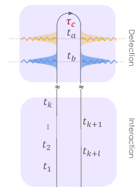
Figure 4: Diagrammatic representation of typical term in Eq. 21. The left (right) branch of the diagram represents the forward (backward) evolution of the joint light-matter wavefunction. The number of interactions in each branch correspond to the respective order of perturbation of either the bra and the ket in the interaction picture. The interaction and detection interval in this calculation do not overlap although in principle the may.

Each term in Eq.21 can be represented using a fully time ordered loop diagram as depicted in Fig. 4. this diagram represents the forward (in time) evolution of the ket (left) pertubatively in the interaction picture to the $k^{\text{th}}$ order, and the bra backwards in time to the $l^{\text{th}}$ order along the time contour $\tau_{C}$. Between interaction events, the sample and the electromagnetic field are evolved using their free Hamiltonian. The lowest order in which two photons interact with the sample and detected is the $4^{\text{th}}$. Contributions with odd number of photons from the left or right at the detection are naturally eliminated. This corresponds to

$${\cal P}\left(\boldsymbol{r}_{a},\boldsymbol{r}_{b};t_{a},t_{b}\right)\approx\sum_{k,l=0}^{4}\langle\Psi^{\left(l\right)}\left(t\right)|E_{-}^{\dagger}\left(\boldsymbol{r}_{b},t_{b}\right)E_{-}^{\dagger}\left(\boldsymbol{r}_{a},t_{a}\right)E_{+}\left(\boldsymbol{r}_{a},t_{a}\right)E_{+}\left(\boldsymbol{r}_{b},t_{b}\right)|\Psi^{\left(k\right)}\left(t\right)\rangle_{\mu\varphi},$$ (22)

where the $\pm$ subscripts highlight the operation direction of the field with respect to the time contour $\tau_{C}$, for positive and negative time direction. Equation 22 gives rise to two kinds of contributions: (1) four interactions in one side and non at the other and (2) two interactions from each side. The Hilbert space description – while equivalent to the alternative Liouville space – results in partial time ordering. The time ordering is maintained along the contour $\tau_{C}$, thus, along the left and right branches of the diagram in Fig. 4individually. Alternatively, if one is interested in evolving the density matrix (in Liouville-space), the relative time-ordering of left and right branches is also important, resulting in absolute time ordering. This difference become important in the interpretation of pertubative treatments of light-matter coupling and essential when one considers coupling to reservoirs. As a result, in the wavefunction approach (Hilbert space) the relative coherence during the evolution is not expressed, only the the final phase accumulated along the entire evolution of the bra and ket separately such that over-all coherence is accounted for as shown in Fig. 5a. Alternatively, in the Liouville-space approach the change in coherence is instantaneously monitored in the calculation process as demonstrated in Fig.5b. For time dependent perturbation theory that includes terms which break time reversal (bath), using the Liouville space approach is inevitable and thus invoked in this paper.

Figure 5: Partial Vs. full time ordering. a) a typical $4^{\text{th}}$ order term in the wavefunction pertubative treatment. b.) Similar terms in Liouville space expansion. Breaking the loop contour (forward and backward) into a single time evolution for both the bra and the ket.

Appendix B The signal

The signal in Eq. 10 is composed of all processes $P_{i}$ evaluated with all observables $O_{j}$. One way to think about it is that each process $P_{i}$ is obtained by coherent superposition of all HOM detection pathways ${\cal C}_{i}\left(t,\tau,T\right)$, and the signal is given by their superposition. The coincidence signal in Eq. 10 can be written accordingly

$${\cal C}\left(t,\tau,T\right)=2\mathfrak{Re}\left\{\sum_{i=1}^{5}{\cal S}_{\nu,i}\right\}$$ (23)

and solved for each detection-interaction pathway combination below separately.

B.1 Example of one process-observable combination

We now illustrate how to combine the preparation and observation boxes for a single term from the total signal. We chose ${\cal S}_{I,1}$ as shown in Fig. 6. This contribution introduces four combinations of field modes corresponding to coupling with $a$ and $b$ modes, $\left(aa,bb,ab,ba\right)$ . We consider the realization in which $a$ is coupled from the left and $b$ from the right.

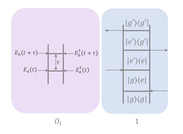
Figure 6: The resulting combination of $\nu=I$ direct detection pathway and $i=1$ interaction pathway.

$${\cal S}_{I,1}|_{a_{L}b_{R}} =\int dt_{4}dt_{3}dt_{2}dt_{1}\theta\left(t_{1}t_{2}\right)\theta\left(t_{2}t_{3}\right)\theta\left(t_{3}t_{4}\right)$$

$$\times\text{tr}\left\{\left[E_{b,R}^{\dagger}\left(t+\tau\right)E_{b,L}\left(t+\tau\right)E_{a,R}^{\dagger}\left(t\right)E_{a,L}\left(t\right)\right]E_{a,L}^{\dagger}\left(t_{1}\right)E_{b,R}\left(t_{2}\right)E_{a,L}\left(t_{3}\right)E_{b,R}^{\dagger}\left(t_{4}\right)\rho_{\varphi}\left(-\infty\right)\right\}$$

$$\times\text{tr}\left\{V_{L}\left(t_{1}\right)V_{R}^{\dagger}\left(t_{2}\right)V_{L}^{\dagger}\left(t_{3}\right)V_{R}\left(t_{4}\right)\rho_{\mu}\left(-\infty\right)\right\}.$$

The operators in the square brackets correspond to the detection process and thus last. Initially, only two fields modes are populated and thus we assume that after the detection process, the field returns to its ground-state (vacuum) and obtain

$${\cal S}_{I,1}|_{b_{L}a_{R}} =\int dt_{4}dt_{3}dt_{2}dt_{1}\theta\left(t_{1}t_{2}\right)\theta\left(t_{2}t_{3}\right)\theta\left(t_{3}t_{4}\right)$$

$$\times\langle\text{vac}|E_{b,L}\left(t+\tau\right)E_{a,L}\left(t\right)E_{b,L}^{\dagger}\left(t_{1}\right)E_{b,L}\left(t_{3}\right)|\Psi_{\theta}\rangle_{\varphi}\langle\Psi_{\theta}|E_{a,R}^{\dagger}\left(t_{4}\right)E_{a,R}\left(t_{2}\right)E_{a,R}^{\dagger}\left(t\right)E_{b,R}^{\dagger}\left(t+\tau\right)|\text{vac}\rangle_{\varphi}$$

$$\times\left\langle V_{L}\left(t_{1}\right)V_{R}^{\dagger}\left(t_{2}\right)V_{L}^{\dagger}\left(t_{3}\right)V_{R}\left(t_{4}\right)\right\rangle_{\mu}.$$

where we have plugged in the explicit expression for the source term $\rho_{\varphi}\equiv|\Psi_{\theta}\rangle\langle\Psi_{\theta}|$. using $\Phi_{\theta}\left(t_{1},t_{2}\right)=\frac{1}{\sqrt{2}}\left[\phi\left(t_{1},t_{2}\right)+e^{-i\theta}\phi\left(t_{2},t_{1}\right)\right]$. Following Ref. [40], we change the integration time variables to time differences between interaction events and obtain

$${\cal S}_{I,1}|_{b_{L}a_{R}} =\int d\tau_{3}d\tau_{4}$$

$$\times\Phi_{\theta}\left(t,t-\tau_{3}\right)\Phi_{\theta}^{*}\left(t,t-\tau_{3}-\tau_{4}\right)$$

$$\times\left\langle V_{L}{\cal G}\left(\tau_{0}\right)V_{R}^{\dagger}{\cal G}\left(\tau_{2}\right)V_{L}^{\dagger}{\cal G}\left(\tau_{3}\right)V_{R}\right\rangle_{\mu},$$

where the Liouville-space Green’s function is given by ${\cal G}\left(t\right)=-\frac{i}{\hbar}\theta\left(t\right)e^{-i{\cal L}_{\mu}t-\eta t}$. This terms was obtained from Eq. 10, using one additional approximation: the free-photon propagator from the sample to the detector is taken to be $\left\langle E_{a,L}\left(t\right)E_{a,L}^{\dagger}\left(t_{1}\right)\right\rangle\approx\delta\left(\Delta t-\nicefrac{{L}}{{c}}\right)$ where $\nicefrac{{L}}{{c}}$ is the distance between the detector and the sample, $c$ is the speed of light and $\Delta t$ is taken to be the time difference between the emission and detection.

Appendix C The final signal – all combinations

Here we combine all possible contributions that correspond to all contributing configurations of the detection and interaction pathways. All pathways are summed as shown in Eq 10.

C.1 ${\cal S}_{\nu,1}$

$${\cal S}_{I,1}= \int d\tau_{3}d\tau_{4}\Phi^{*}\left(t-\tau_{3:4},t+\tau_{0}\right)\Phi\left(t,t-\tau_{3}\right){\cal F}_{1}\left(\tau_{0},\tau_{3},\tau_{4}\right)$$

$${\cal S}_{II,1}: \int d\tau_{3}d\tau_{4}\Phi^{*}\left(t+\tau_{0},t-\tau_{3:4}\right)\Phi\left(t-\tau_{3},t\right){\cal F}_{1}\left(\tau_{0},\tau_{3},\tau_{4}\right)$$

$${\cal S}_{III,1}=- \int d\tau_{3}d\tau_{4}\Phi^{*}\left(t,t+\tau_{0}-\tau_{3:4}\right)\Phi\left(t+\tau_{0}-\tau_{3},t-T\right){\cal F}_{1}\left(T,\tau_{3},\tau_{4}\right)$$

$$- \int d\tau_{3}d\tau_{4}\Phi^{*}\left(t-\tau_{3:4},t+\tau_{0}\right)\Phi\left(t-\tau_{3},t-T\right){\cal F}_{1}\left(T+\tau_{0},\tau_{3},\tau_{4}\right)$$

$${\cal S}_{IV,1}=- \int d\tau_{3}d\tau_{4}\Phi^{*}\left(t+T+\tau,t-T-\tau_{3:4}\right)\Phi\left(t-T-\tau_{3},t+\tau_{0}\right){\cal F}_{1}\left(T,\tau_{3},\tau_{4}\right)$$

$$- \int d\tau_{3}d\tau_{4}\Phi^{*}\left(t+T+\tau,t-T-\tau_{3:4}\right)\Phi\left(t,t-T-\tau_{3}\right){\cal F}_{1}\left(\tau_{0}+T,\tau_{3},\tau_{4}\right)$$

C.2 ${\cal S}_{\nu,2}$

$${\cal S}_{I,2}= \int d\tau_{3}d\tau_{4}\Phi^{*}\left(t-\tau_{4},t+\tau_{0}\right)\Phi\left(t,t+\tau_{3}\right){\cal F}_{2}\left(\tau_{0}-\tau_{3},\tau_{3},\tau_{4}\right)$$

$${\cal S}_{II,2}= \int d\tau_{3}d\tau_{4}\Phi^{*}\left(t+\tau_{0},t-\tau_{4}\right)\Phi\left(t+\tau_{3},t\right){\cal F}_{2}\left(\tau_{0}-\tau_{3},\tau_{3},\tau_{4}\right)$$

$${\cal S}_{III,2} =-\int d\tau_{3}d\tau_{4}\Phi^{*}\left(t,t+\tau_{0}-\tau_{4}\right)\Phi\left(t+\tau_{0}+\tau_{3},t-T\right){\cal F}_{2}\left(T-\tau_{3},\tau_{3},\tau_{4}\right)$$

$$-\int d\tau_{3}d\tau_{4}\Phi^{*}\left(t-\tau_{4},t+\tau_{0}\right)\Phi\left(t+\tau_{3},t-T\right){\cal F}_{2}\left(\tau_{0}+T-\tau_{3},\tau_{3},\tau_{4}\right)$$

$${\cal S}_{IV,2}=- \int d\tau_{3}d\tau_{4}\Phi^{*}\left(t+T+\tau,t-T-\tau_{4}\right)\Phi\left(t-T+\tau_{3},t+\tau_{0}\right){\cal F}_{2}\left(T-\tau_{3},\tau_{3},\tau_{4}\right)$$

$$- \int d\tau_{3}d\tau_{4}\Phi^{*}\left(t+T+\tau,t-T-\tau_{4}\right)\Phi\left(t,t-T+\tau_{3}\right){\cal F}_{2}\left(\tau_{0}+T-\tau_{3},\tau_{3},\tau_{4}\right)$$

C.3 ${\cal S}_{\nu,3}$

$${\cal S}_{I,3}= \int d\tau_{3}d\tau_{4}\Phi^{*}\left(t-\tau_{3},t+\tau_{0}\right)\Phi\left(t,t-\tau_{3:4}\right){\cal F}_{3}\left(\tau_{0},\tau_{3},\tau_{4}\right)$$

$${\cal S}_{II,3}= \int d\tau_{3}d\tau_{4}\Phi^{*}\left(t+\tau_{0},t-\tau_{3}\right)\Phi\left(t-\tau_{3:4},t\right){\cal F}_{3}\left(\tau_{0},\tau_{3},\tau_{4}\right)$$

$${\cal S}_{III,3}=- \int d\tau_{3}d\tau_{4}\Phi^{*}\left(t,t+\tau_{0}-\tau_{3}\right)\Phi\left(t+\tau_{0}-\tau_{3:4},t-T\right){\cal F}_{3}\left(T,\tau_{3},\tau_{4}\right)$$

$$- \int d\tau_{3}d\tau_{4}\Phi^{*}\left(t-\tau_{3},t+\tau_{0}\right)\Phi\left(t-\tau_{3:4},t-T\right){\cal F}_{3}\left(\tau_{0}+T,\tau_{3},\tau_{4}\right)$$

$${\cal S}_{IV,3}=- \int d\tau_{3}d\tau_{4}\Phi^{*}\left(t+T+\tau,t-T-\tau_{3}\right)\Phi\left(t-T-\tau_{3:4},t+\tau_{0}\right){\cal F}_{3}\left(T,\tau_{3},\tau_{4}\right)$$

$$- \int d\tau_{3}d\tau_{4}\Phi^{*}\left(t+T+\tau,t-T-\tau_{3}\right)\Phi\left(t,t-T-\tau_{3:4}\right){\cal F}_{3}\left(T+\tau_{0},\tau_{3},\tau_{4}\right)$$

C.4 ${\cal S}_{\nu,4}$

$${\cal S}_{I,4}= \int d\tau_{3}d\tau_{4}\Phi^{*}\left(t,t+\tau_{0}\right)\Phi\left(t-\tau_{4},t+\tau_{3}\right){\cal F}_{4}\left(\tau_{0}-\tau_{3},\tau_{3},\tau_{4}\right)$$

$${\cal S}_{II,4} =\int d\tau_{3}d\tau_{4}\Phi^{*}\left(t+\tau_{0},t\right)\Phi\left(t+\tau_{0}+\tau_{3},t+\tau_{0}-\tau_{4}\right){\cal F}_{4}\left(\tau_{0}-\tau_{3},\tau_{3},\tau_{4}\right)$$

$${\cal S}_{III,4}=- \int d\tau_{3}d\tau_{4}\Phi^{*}\left(t,t+\tau_{0}\right)\Phi\left(t-T+\tau_{3},t-T-\tau_{4}\right){\cal F}_{4}\left(2T+\tau_{0}-\tau_{3},\tau_{3},\tau_{4}\right)$$

$${\cal S}_{IV,4}=- \int d\tau_{3}d\tau_{4}\Phi^{*}\left(t+T+\tau,t-T\right)\Phi\left(t-\tau_{4},t+\tau_{3}\right){\cal F}_{4}\left(\tau_{0}-\tau_{3},\tau_{3},\tau_{4}\right)$$

C.5 ${\cal S}_{\nu,5}$

Here, each contribution is naturally symmetrized.

$${\cal S}_{I,5}=\int d\tau_{3}d\tau_{4}\Phi^{*}\left(t,t+\tau_{0}\right)\left[\Phi_{ab}\left(t-\tau_{3},t-\tau_{3:4}\right)+\Phi_{ba}\right]{\cal F}_{5}\left(\tau_{0},\tau_{3},\tau_{4}\right)$$

$${\cal S}_{II,5}=\int d\tau_{3}d\tau_{4}\Phi^{*}\left(t+\tau_{0},t\right)\left[\Phi_{ab}\left(t-\tau_{3},t-\tau_{3:4}\right)+\Phi_{ba}\right]{\cal F}_{5}\left(\tau_{0},\tau_{3},\tau_{4}\right)$$

$${\cal S}_{III,5}=-\int d\tau_{3}d\tau_{4}\Phi^{*}\left(t,t+\tau_{0}\right)\left[\Phi_{ab}\left(t-T-\tau_{3:4},t-T-\tau_{3}\right)+\Phi_{ba}\right]{\cal F}_{5}\left(\tau_{0}+2T,\tau_{3},\tau_{4}\right)$$

$${\cal S}_{IV,5}=-\int d\tau_{3}d\tau_{4}\Phi^{*}\left(t+T+\tau_{0},t-T\right)\left[\Phi_{ab}\left(t-\tau_{3},t-\tau_{3:4}\right)+\Phi_{ba}\right]{\cal F}_{5}\left(\tau_{0},\tau_{3},\tau_{4}\right)$$