Natural Language Descriptions of
Deep Visual Features

Abstract

Some neurons in deep networks specialize in recognizing highly specific perceptual, structural, or semantic features of inputs. In computer vision, techniques exist for identifying neurons that respond to individual concept categories like colors, textures, and object classes. But these techniques are limited in scope, labeling only a small subset of neurons and behaviors in any network. Is a richer characterization of neuron-level computation possible? We introduce a procedure (called milan, for mutual-information-guided linguistic annotation of neurons) that automatically labels neurons with open-ended, compositional, natural language descriptions. Given a neuron, milan generates a description by searching for a natural language string that maximizes pointwise mutual information with the image regions in which the neuron is active. milan produces fine-grained descriptions that capture categorical, relational, and logical structure in learned features. These descriptions obtain high agreement with human-generated feature descriptions across a diverse set of model architectures and tasks, and can aid in understanding and controlling learned models. We highlight three applications of natural language neuron descriptions. First, we use milan for analysis, characterizing the distribution and importance of neurons selective for attribute, category, and relational information in vision models. Second, we use milan for auditing, surfacing neurons sensitive to human faces in datasets designed to obscure them. Finally, we use milan for editing, improving robustness in an image classifier by deleting neurons sensitive to text features spuriously correlated with class labels.

1 Introduction

A surprising amount can be learned about the behavior of a deep network by understanding the individual neurons that make it up. Previous studies aimed at visualizing or automatically categorizing neurons have identified a range of interpretable functions across models and application domains: low-level convolutional units in image classifiers implement color detectors and Gabor filters (Erhan et al., 2009), while some later units activate for specific parts and object categories (Zeiler & Fergus, 2014; Bau et al., 2017). Single neurons have also been found to encode sentiment in language data (Radford et al., 2017) and biological function in computational chemistry (Preuer et al., 2019). Given a new model trained to perform a new task, can we automatically catalog these behaviors?

Techniques for characterizing the behavior of individual neurons are still quite limited. Approaches based on visualization (Zeiler & Fergus, 2014; Girshick et al., 2014; Karpathy et al., 2015; Mahendran & Vedaldi, 2015; Olah et al., 2017) leave much of the work of interpretation up to human users, and cannot be used for large-scale analysis. Existing automated labeling techniques (Bau et al., 2017; 2019; Mu & Andreas, 2020) require researchers to pre-define a fixed space of candidate neuron labels; they label only a subset of neurons in a given network and cannot be used to surface novel or unexpected behaviors.

This paper develops an alternative paradigm for labeling neurons with expressive, compositional, and open-ended annotations in the form of natural language descriptions. We focus on the visual domain: building on past work on information-theoretic approaches to model interpretability, we formulate neuron labeling as a problem of finding informative descriptions of a neuron’s pattern of activation on input images. We describe a procedure (called milan, for mutual-information-guided linguistic annotation of neurons) that labels individual neurons with fine-grained natural language descriptions by searching for descriptions that maximize pointwise mutual information with the image regions in which neurons are active. To do so, we first collect a new dataset of fine-grained image annotations (milannotations, Figure 1c), then use these to construct learned approximations to the distributions over image regions (Figure 1b) and descriptions. In some cases, milan surfaces neuron descriptions that more specific than the underlying training data (Figure 1d).

milan is largely model-agnostic and can surface descriptions for different classes of neurons, ranging from convolutional units in CNNs to fully connected units in vision transformers, even when the target network is trained on data that differs systematically from milannotations’ images. These descriptions can in turn serve a diverse set of practical goals in model interpretability and dataset design. Our experiments highlight three: using milan-generated descriptions to (1) analyze the role and importance of different neuron classes in convolutional image classifiers, (2) audit models for demographically sensitive feature by comparing their features when trained on anonymized (blurred) and non-anonymized datasets, and (3) identify and mitigate the effects of spurious correlations with text features, improving classifier performance on adversarially distributed test sets. Taken together, these results show that fine-grained, automatic annotation of deep network models is both possible and practical: rich descriptions produced by automated annotation procedures can surface meaningful and actionable information about model behavior.

Figure 1: (a) We aim to generate natural language descriptions of individual neurons in deep networks. (b) We first represent each neuron via an exemplar set of input regions that activate it. (c) In parallel, we collect a dataset of fine-grained human descriptions of image regions, and use these to train a model of $p(\textrm{description}\mid\text{exemplars})$ and $p(\textrm{description})$. (d) Using these models, we search for a description that has high pointwise mutual information with the exemplars, ultimately generating highly specific neuron annotations.

2 Related Work

Interpreting deep networks

milan builds on a long line of recent approaches aimed at explaining the behavior of deep networks by characterizing the function of individual neurons, either by visualizing the inputs they select for (Zeiler & Fergus, 2014; Girshick et al., 2014; Karpathy et al., 2015; Mahendran & Vedaldi, 2015; Olah et al., 2017) or by automatically categorizing them according to the concepts they recognize (Bau et al., 2017; 2018; Mu & Andreas, 2020; Morcos et al., 2018; Dalvi et al., 2019). Past approaches to automatic neuron labeling require fixed, pre-defined label sets; in computer vision, this has limited exploration to pre-selected object classes, parts, materials, and simple logical combinations of these concepts. While manual inspection of neurons has revealed that a wider range of features play an important role in visual recognition (e.g. orientation, illumination, and spatial relations; Cammarata et al. 2021) milan is the first automated approach that can identify such features at scale. Discrete categorization is also possible for directions in representation space (Kim et al., 2018; Andreas et al., 2017; Schwettmann et al., 2021) and for clusters of images induced by visual representations (Laina et al., 2020); in the latter, an off-the-shelf image captioning model is used to obtain language descriptions of the unifying visual concept for the cluster, although the descriptions miss low-level visual commonalities. As milan requires only a primitive procedure for generating model inputs maximally associated with the feature or direction of interest, future work might extend it to these settings as well.

Natural language explanations of decisions

Previous work aimed at explaining computer vision classifiers using natural language has focused on generating explanations for individual classification decisions (e.g., Hendricks et al., 2016; Park et al., 2018; Hendricks et al., 2018; Zellers et al., 2019). Outside of computer vision, several recent papers have proposed procedures for generating natural language explanations of decisions in text classification models (Zaidan & Eisner, 2008; Camburu et al., 2018; Rajani et al., 2019; Narang et al., 2020) and of representations in more general sequence modeling problems (Andreas & Klein, 2017). These approaches require task-specific datasets and often specialized training procedures, and do not assist with interpretability at the model level. To the best of our knowledge, milan is the first approach for generating compositional natural language descriptions for interpretability at the level of individual features rather than input-conditional decisions or representations. More fundamentally, milan can do so independently of the model being described, making it (as shown in Section 4) modular, portable, and to a limited extent task-agnostic.

3 Approach

Neurons and exemplars

Consider the neuron depicted in Figure 1b, located in a convlutional network trained to classify scenes (Zhou et al., 2017). When the images in Figure 1 are provided as input to the network, the neuron activates in patches of grass near animals, but not in grass without animals nearby. How might we automate the process of automatically generating such a description?

While the image regions depicted in Fig. 1b do not completely characterize the neuron’s function in the broader network, past work has found that actionable information can be gleaned from such regions alone. Bau et al. (2020; 2019) use them to identify neurons that can trigger class predictions or generative synthesis of specific objects; Andreas & Klein (2017) use them to predict sequence outputs on novel inputs; Olah et al. (2018) and Mu & Andreas (2020) use them to identify adversarial vulnerabilities. Thus, building on this past work, our approach to neuron labeling also begins by representing each neuron via the set of input regions on which its activity exceeds a fixed threshold.

Definition 1.

Let $f:X\to Y$ be a neural network, and let $f_{i}(x)$ denote the activation value of the $i$th neuron in $f$ given an input $x$. Then, an exemplar representation of the neuron $f_{i}$ is given by:

$$E_{i}=\{x\in X:f_{i}(x)>\eta_{i}\}~{}.$$ (1)

for some threshold parameter $\eta_{i}$ (discussed in more detail below).

Exemplars and descriptions

Given this explicit representation of $f_{i}$’s behavior, it remains to construct a description $d_{i}$ of the neuron. Past work (Bau et al., 2017; Andreas et al., 2017) begins with a fixed inventory of candidate descriptions (e.g. object categories), defines an exemplar set $E^{\prime}_{d}$ for each such category (e.g. via the output of a semantic segmentation procedure) then labels neurons by optimizing $d_{i}:=\operatorname*{arg\,min}_{d}~{}\delta(E_{i},E^{\prime}_{d})$ for some measure of set distance (e.g. Jaccard, 1912).

In this work, we instead adopt a probabilistic approach to neuron labeling. In computer vision applications, each $E_{i}$ is a set of image patches. Humans are adept at describing such patches (Rashtchian et al., 2010) and one straightforward possibility might be to directly optimize $d_{i}:=\operatorname*{arg\,max}_{d}~{}p(d\mid E_{i})$. In practice, however, the distribution of human descriptions given images may not be well-aligned with the needs of model users. Fig. 2 includes examples of human-generated descriptions for exemplar sets. Many of them (e.g. text for AlexNet conv3-252) are accurate, but generic; in reality, the neuron responds specifically to text on screens. The generated description of a neuron should capture the specificity of its function—especially relative to other neurons in the same model.

We thus adopt an information-theoretic criterion for selecting descriptions: our final neuron description procedure optimizes pointwise mutual information between descriptions and exemplar sets:

Definition 2.

The max-mutual-information description of the neuron $f_{i}$ is given by:

$$\textsc{milan}(f_{i}):=\operatorname*{arg\,max}_{d}~{}\mathrm{pmi}(d;E_{i})=\operatorname*{arg\,max}_{d}~{}\log p(d\mid E_{i})-\log p(d)~{}.$$ (2)

To turn Eq. 2 into a practical procedure for annotating neurons, three additional steps are required: constructing a tractable approximation to the exemplar set $E_{i}$ (Section 3.1), using human-generated image descriptions to model $p(d\mid E)$ and $p(d)$ (Section 3.2 and Section 3.3), and finding a high-quality description $d$ in the infinite space of natural language strings (Section 3.4).

Figure 2: Examples of milan descriptions on the generalization tasks described in Section 4. Even highly specific labels (like the top boundaries of horizontal objects) can be predicted for neurons in new networks. Failure modes include semantic errors, e.g. milan misses the cupcakes in the dog faces and cupcakes neuron.

3.1 Approximating the exemplar set

As written, the exemplar set in Equation 1 captures a neuron’s behavior on all image patches. This set is large (limited only by the precision used to represent individual pixel values), so we follow past work (Bau et al., 2017) by restricting each $E_{i}$ to the set of images that cause the greatest activation in the neuron $f_{i}$. For convolutional neurons in image processing tasks, sets $E_{i}$ ultimately comprise $k$ images with activation masks indicating the regions of those images in which $f_{i}$ fired (Fig. 1a; see Bau et al. 2017 for details). Throughout this paper, we use exemplar sets with $k=15$ images and choose $\eta_{i}$ equal to the 0.99 percentile of activations for the neuron $f_{i}$.

3.2 Modeling $p(d\mid E)$ and $p(d)$

The term $\mathrm{pmi}(d;E_{i})$ in Equation 2 can be expressed in terms of two distributions: the probability $p(d\mid E_{i})$ that a human would describe an image region with $d$, and the probability $p(d)$ that a human would use the description $d$ for any neuron. $p(d\mid E_{i})$ is, roughly speaking, a distribution over image captions (Donahue et al., 2015). Here, however, the input to the model is not a single image but a set of image regions (the masks in Fig. 1a); we seek natural language descriptions of the common features of those regions. We approximate $p(d\mid E_{i})$ with learned model—specifically the Show-Attend-Tell image description model of Xu et al. (2015) trained on the milannotations dataset described below, and with several modifications tailored to our use case. We approximate $p(d)$ with a two-layer LSTM language model (Hochreiter & Schmidhuber, 1997) trained on the text of milannotations. Details about both models are provided in Appendix B.

3.3 Collecting human annotations

As $p(d\mid E_{i})$ and $p(d)$ are both estimated using learned models, they require training data. In particular, modeling $p(d\mid E_{i})$ requires a dataset of captions that describe regions from multiple different images, such as the ones shown in Fig. 1. These descriptions must describe not only objects and actions, but all other details that individual neurons select for. Existing image captioning datasets, like MSCOCO (Lin et al., 2014) and Conceptual Captions (Sharma et al., 2018), only focus on scene-level details about a single image and do not provide suitable annotations for this task. We therefore collect a novel dataset of captions for image regions to train the models underlying milan.

Network	Arch.	Task	Datasets	Annotated	# Units
AlexNet	CNN	Class.	ImageNet Places365	conv. 1–5	1152 1376
ResNet152	CNN	Class.	ImageNet Places365	conv. 1 res. 1–4	3904 3904
BigGAN	CNN	Gen.	ImageNet Places365	res. 0–5	3744 4992
DINO	ViT	BYOL	ImageNet	MLP 1–12 (first 100)	1200

Table 1: Summary of milannotations, which labels 20k units across 7 models with different network architectures, datsasets, and tasks. Each unit is annotated by three human participants.

First, we must obtain a set of image regions to annotate. To ensure that these regions have a similar distribution to the target neurons themselves, we derive them directly from the exemplar sets of neurons in a set of seed models. We obtain the exemplar sets for a subset of the units in each seed model in Table 1 using the method from Section 3.1. We then present each set to a human annotator and ask them to describe what is common to the image regions.

Table 1 summarizes the dataset, which we call milannotations. In total, we construct exemplar sets using neurons from seven vision models, totaling 20k neurons. These models include two architectures for supervised image classification, AlexNet (Krizhevsky et al., 2012) and ResNet152 (He et al., 2015); one architecture for image generation, BigGAN (Brock et al., 2018); and one for unsupervised representation learning trained with a “Bootsrap Your Own Latent” (BYOL) objective (Chen & He, 2020; Grill et al., 2020), DINO (Caron et al., 2021). These models cover two datasets, specifically ImageNet (Deng et al., 2009) and Places365 (Zhou et al., 2017), as well as two completely different families of models, CNNs and Vision Transformers (ViT) (Dosovitskiy et al., 2021). Each exemplar set is shown to three distinct human participants, resulting 60k total annotations. Examples are provided in Appendix A (Fig. 10). We recruit participants from Amazon Mechanical Turk. This data collection effort was approved by MIT’s Committee on the Use of Humans as Experimental Subjects. To control for quality, workers were required to have a HIT acceptance rate of at least 95%, have at least 100 approved HITs, and pass a short qualification test. Full details about our data collection process and the collected data can be found in Appendix A.

3.4 Searching in the space of descriptions

Directly decoding descriptions from $\mathrm{pmi}(d;E_{i})$ tends to generate disfluent descriptions. This is because the $p(d)$ term inherently discourages common function words like the from appearing in descriptions. Past work language generation (Wang et al., 2020) has found that this can be remedied by first introducing a hyperparameter $\lambda$ to modulate the importance of $p(d)$ when computing PMI, giving a new weighted PMI objective:

$$\mathrm{wpmi}(d)=\log p(d\mid E_{i})-\lambda\log p(d).$$ (3)

Next, search is restricted to a set of captions that are high probability under $p(d\mid E_{i})$, which are reranked according to Eq. 3. Specifically, we run beam search on $p(d\mid E_{i})$, and use the full beam after the final search step as a set of candidate descriptions. For all experiments, we set $\lambda=.2$ and beam size to 50.

4 Does milan generalize?

Because it is trained on a set of human-annotated exemplar sets obtained from a set of seed networks, milan is useful as an automated procedure only if it generalizes and correctly describes neurons in trained models with new architectures, new datasets, and new training objectives. Thus, before describing applications of milan to specific interpretability problems, we perform cross-

Model	CE	ND	$p(d\mid E)$	$\mathrm{pmi}(d;E)$
AlexNet-ImageNet	.01	.24	.34	.38
AlexNet-Places	.02	.21	.31	.37
ResNet-ImageNet	.01	.25	.27	.35
ResNet-Places	.03	.22	.30	.31

Table 2: BERTScores for neuron labeling methods relative to human annotations. milan obtains higher agreement than Compositional Explanations (CE) or NetDissect (ND).

validation experiments within the milannotations data to validate that milan can reliably label new neurons. We additionally verify that milan provides benefits over other neuron annotation techniques by comparing its descriptions to three baselines: NetDissect (Bau et al., 2017), which assigns a single concept label to each neuron by comparing the neuron’s exemplars to semantic segmentations of the same images; Compositional

Generalization	Train + Test	BERTScore (f)
within network	AlexNet–ImageNet		.39
	AlexNet–Places		.47
	ResNet152–ImageNet		.35
	ResNet152–Places		.28
	BigGAN–ImageNet		.49
	BigGAN–Places		.52
	Train	Test
across arch.	AlexNet	ResNet152	.28
	ResNet152	AlexNet	.35
	CNNs	ViT	.34
across datasets	ImageNet	Places	.30
	Places	ImageNet	.33
across tasks	Classifiers	BigGAN	.34
	BigGAN	Classifiers	.27

Table 3: BERTScores on held out neurons relative to the human annotations. Each train/test split evaluates a different kind of generalization, ultimately evaluating how well milan generalizes to networks with architectures, datasets, and tasks unseen in the training annotations.

Explanations (Mu & Andreas, 2020), which follows a similar procedure to generate logical concept labels; and ordinary image captioning (selecting descriptions using $p(d\mid E)$ instead of $\mathrm{pmi}(d;E)$).

Method

In each experiment, we train milan on a subset of milannotations and evaluate its performance on a held-out subset. To compare milan to the baselines, we train on all data except a single held-out network; we obtain the baseline labels by running the publicly available code with the default settings on the held-out network. To test generalization within a network, we train on 90% of neurons from each network and test on the remaining 10%. To test generalization across architectures, we train on all AlexNet (ResNet) neurons and test on all ResNet (AlexNet) neurons; we also train on all CNN neurons and test on ViT neurons. To test generalization across datasets, we train on all neurons from models trained on ImageNet (Places) and test on neurons from models for the other datasets. To test generalization across tasks, we train on all classifier neurons (GAN neurons) and test on all GAN neurons (classifier neurons). We measure performance via BERTScore (Zhang et al., 2020) relative to the human annotations. Hyperparameters for each of these experiments are in Appendix C.

Results

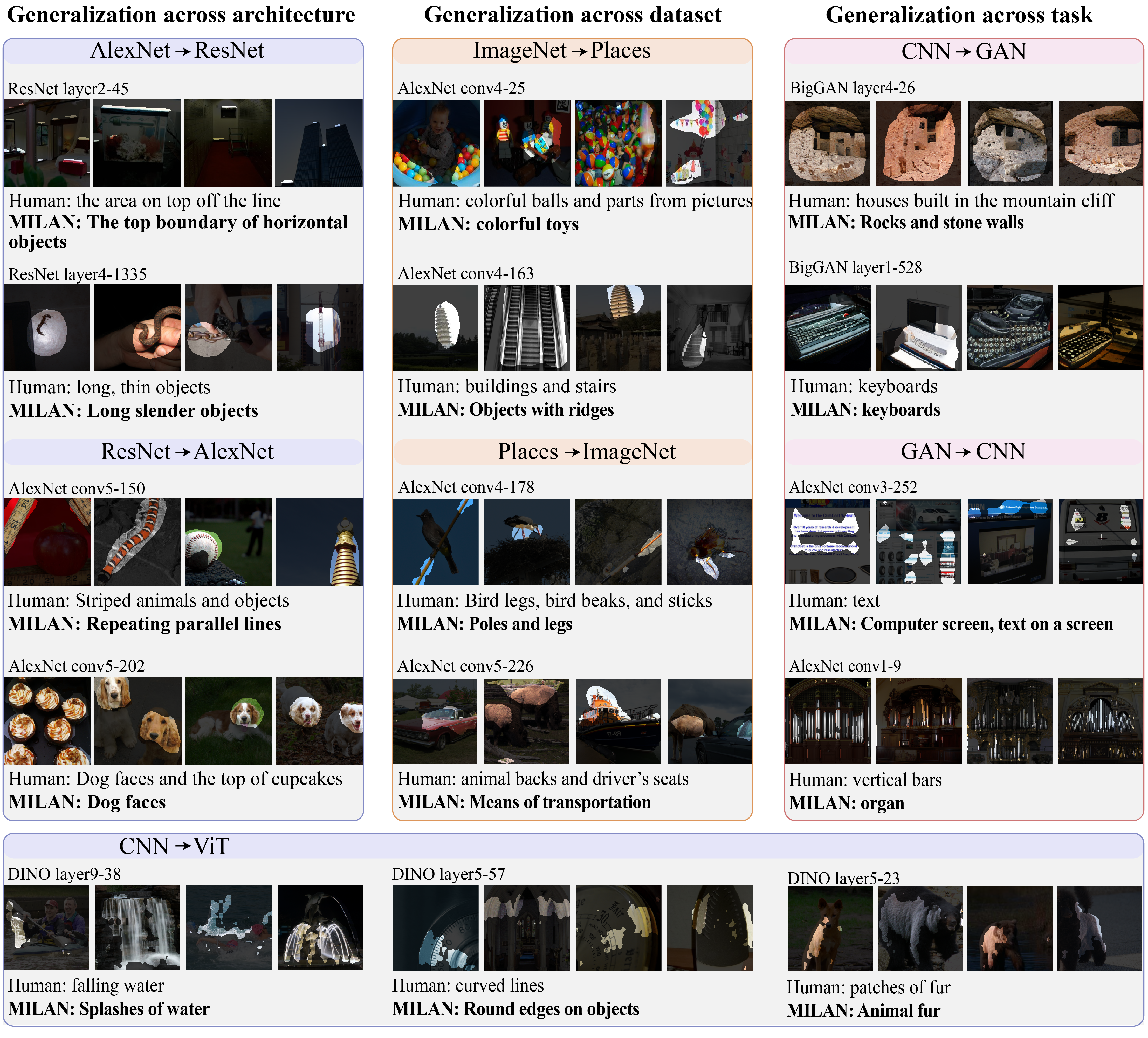
Table 2 shows results for milan and all three baselines applied to four different networks. milan obtains higher agreement with human annotations on held-out networks than baselines. It is able to surface highly specific behaviors in its descriptions, like the splashes of water neuron shown in Figure 2 (splashes has no clear equivalent in the concept sets used by NetDissect (ND) or Compositional Explanations (CE)). milan also outperforms the ablated $p(d\mid E)$ decoder, justifying the choice of $\mathrm{pmi}$ as an objective for obtaining specific and high-quality descriptions.

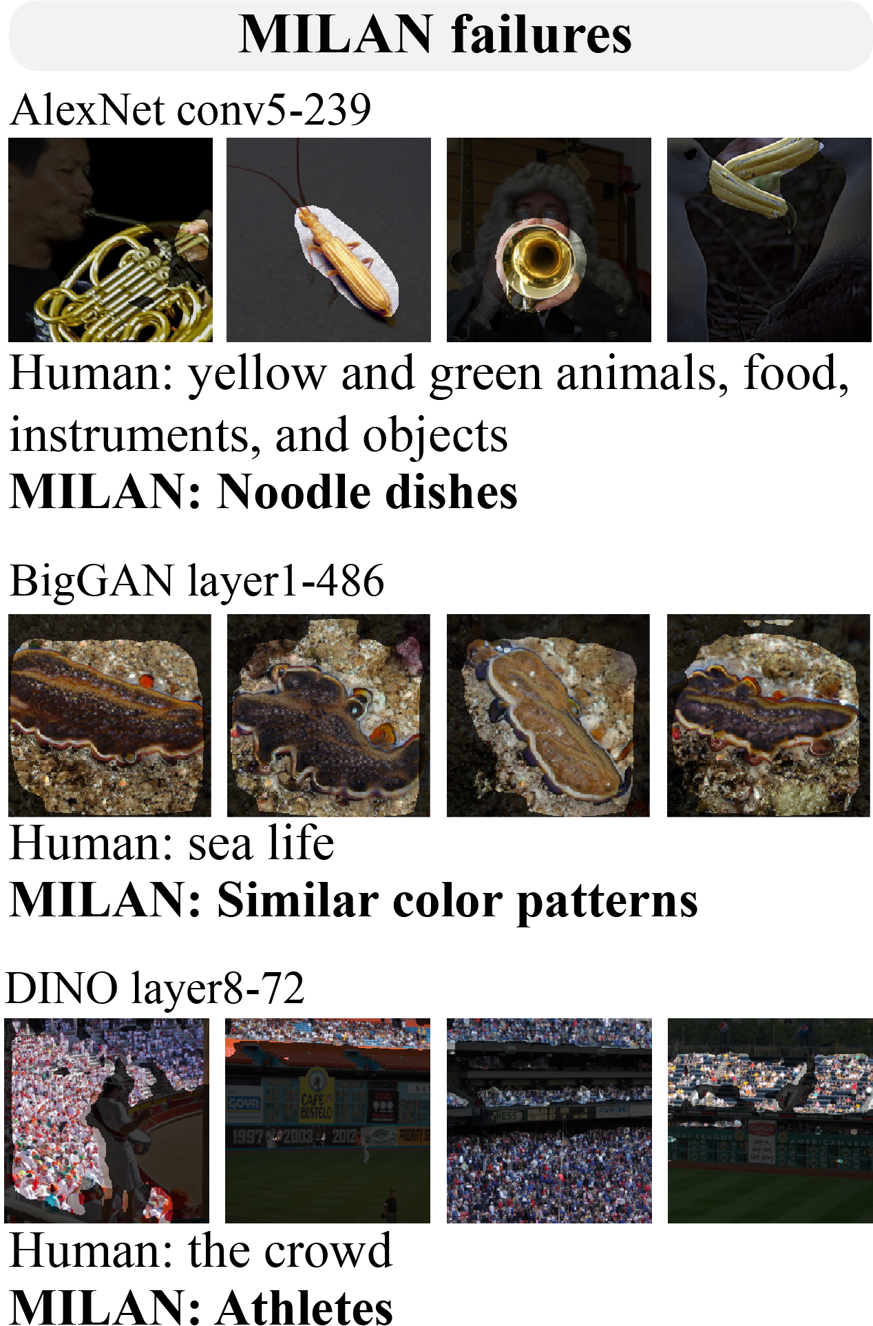
Table 3 shows that milan exhibits different degrees of generalization across models, with generalization to new GAN neurons in the same network easiest and GAN-to-classifier generalization hardest. milan can generalize to novel architectures. It correctly labels ViT neurons (in fully connected layers) as often as it correctly labels other convolutional units (e.g., in AlexNet). We observe that transferability across tasks is asymmetric: agreement scores are higher when transferring from classifier neurons to GAN neurons than the reverse. Finally, Figure 3 presents some of milan’s failure cases: when faced with new visual concepts, milan sometimes mislabels the concept (e.g., by calling brass instruments noodle dishes), prefers a vague description (e.g., similar color patterns), or ignores the highlighted regions and describes the context instead.

We emphasize that this section is primarily intended as a sanity check of the learned models underlying milan, and not as direct evidence of its usefulness or reliability as a tool for interpretability. We

Figure 3: Examples of milan failures. Failure modes include incorrect generalization (top), vague descriptions for concepts not seen in the training set (middle), and mistaking the context for the highlighted regions (bottom).

follow Vaughan & Wallach (2020) in arguing that the final test of any such tool must be its ability to produce actionable insights for human users, as in the three applications described below.

5 Analyzing Feature Importance

The previous section shows that milan can generalize to new architectures, datasets, and tasks. The remainder of this paper focuses on applications that use generated labels to understand how neurons influence model behavior. As a first example: descriptions in Figure 2 reveal that neurons have different degrees of specificity. Some neurons detect objects with spatial constraints (the area on top of the line), while others fire for low-level but highly specific perceptual qualities (long, thin objects). Still others detect perceptually similar but fundamentally different objects (dog faces and cupcakes). How important are these different classes of neurons to model behavior?

Method

(a)

(b)

(c)

Figure 4: ResNet18 accuracy on the ImageNet validation set as units are ablated (left, middle), and distribution of neurons matching syntactic and structural criteria in each layer (right). In each configuration, neurons are scored according to a property of their generated description (e.g., number of nouns/words in description, etc.), sorted based on their score, and ablated in that order. Neurons described with adjectives appear crucial for good performance, while neurons described with very different words (measured by word embedding difference; max word diff.) appear less important for good performance. Adjective-selective neurons are most prevalent in early layers, while neurons with large semantic differences are more prevalent in late ones.

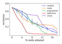
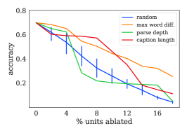
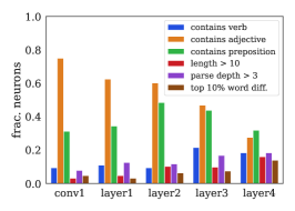
We use milan trained on all convolutional units in milannotations to annotate every neuron in ResNet18-ImageNet. We then score each neuron according to one of seven criteria that capture different syntactic or structural properties of the caption. Four syntactic criteria each count the number of times that a specific part of speech appears in a caption: nouns, verbs, prepositions, and adjectives. Three structural criteria measure properties of the entire caption: its length, the depth of its parse tree (a rough measure of its compositional complexity, obtained from the spaCy parser of Honnibal et al. 2020), and its maximum word difference (a measure of the semantic coherence of the description, measured as the maximum Euclidean distance between any two caption words, again obtained via spaCy). Finally, neurons are incrementally ablated in order of their score. The network is tested on the ImageNet validation set and its accuracy recorded. This procedure is then repeated, deleting 2% of neurons at each step. We also include five trials in which neurons are ordered randomly. Further details and examples of ablated neurons are provided in Appendix D.

Results

Figure 4 plots accuracy on the ImageNet validation set as a function of the number of ablated neurons. Linguistic features of neuron descriptions highlight several important differences between neurons. First, neurons captioned with many adjectives or prepositions (that is, neurons that capture attributes and relational features) are relatively important to model behavior. Ablating these neurons causes a rapid decline in performance compared to ablating random neurons or nouns. Second, neurons that detect dissimilar concepts appear to be less important. When the caption contains highly dissimilar words (max word diff.), ablation hurts performance substantially less than ablating random neurons. Such neurons sometimes detect non-semantic compositions of concepts like the dog faces and cupcakes neuron shown in Fig. 2; Mu & Andreas (2020) find that these units contribute to non-robust model behavior. We reproduce their robustness experiments using these neurons in Section 5 (Figure 14) and reach similar conclusions. Finally, Figure 4 highlights that neurons satisfying each criterion are not evenly distributed across layers—for example, middle layers contain the largest fraction of relation-selective neurons measured via prepositions.

6 Auditing Anonymized Models

One recent line of work in computer vision aims to construct privacy-aware datasets, e.g. by detecting and blurring all faces to avoid leakage of information about specific individuals into trained models (Yang et al., 2021). But to what extent does this form of anonymization actually reduce

Figure 5: Change in # of face neurons found by milan (each pair of points is one model architecture). Blurring reduces, but does not eliminate, units selective for unblurred faces.

models’ reliance on images of humans? We wish to understand if models trained on blurred data still construct features that can human faces, or even specific categories of faces. A core function of tools for interpretable machine learning is to enable auditing of trained models for such behavior; here, we apply milan to investigate the effect of blurring-based dataset privacy.

Figure 6: (a) The blurred ImageNet dataset. (b–c) Exemplar sets and labels for two neurons in a blurred model that activate on unblurred faces—and appear to preferentially (but not exclusively) respond to faces in specific demographic categories.

Method

We use milan to caption a subset of convolutional units in 12 different models pretrained for image classification on the blurred ImageNet images (blurred models). These models are distributed by the original authors of the blurred ImageNet dataset (Yang et al., 2021). We caption the same units in models pretrained on regular ImageNet (unblurred models) obtained from torchvision (Paszke et al., 2019). We then manually inspect all neurons in the blurred and unblurred models for which milan descriptions contain the words face, head, nose, eyes, and mouth (using exemplar sets containing only unblurred images).

Results

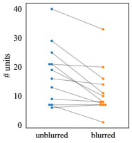
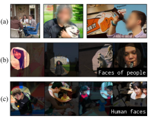
Across models trained on ordinary ImageNet, milan identified 213 neurons selective for human faces. Across models trained on blurred ImageNet, milan identified 142 neurons selective for human faces. milan can distinguish between models trained on blurred and unblurred data (Fig. 5). However, it also reveals that models trained on blurred data acquire neurons selective for unblurred faces. Indeed, it is possible to use milan’s labels to extract these face-selective neurons directly. Doing so reveals that several of them are not simply face detectors, but appear to selectively identify female faces (Fig. 6b) and Asian faces (Fig. 6c). Blurring does not prevent models from extracting highly specific features for these attributes. Our results in this section highlight the use of milan for both quantitative and qualitative, human-in-the loop auditing of model behavior.

7 Editing Spurious Features

Spurious correlations between features and labels are a persistent problem in machine learning applications, especially in the presence of mismatches between training and testing data (Storkey, 2009). In object recognition, one frequent example is correlation between backgrounds and objects (e.g. cows are more likely to appear with green grass in the background, while fish are more likely to appear with a blue background; Xiao et al. 2020). In a more recent example, models trained on joint text and image data are subject to “text-based adversarial attacks”, in which e.g. an apple with the word iPod written on it is classified as an iPod (Goh et al., 2021). Our final experiment shows that milan can be used to reduce models’ sensitivity to these spurious features.

Figure 7: Network editing. (a) We train an image classifier on a synthetic dataset in which half the images include the class label written in text in the corner. (b) We evaluate the classifier on an adversarial test set, in which every image has a random textual label. (c) Nearly a third of neurons in the trained model model detect text, hurting its performance on the test set.

Data

We create a controlled dataset imitating Goh et al. (2021)’s spurious text features. The dataset consists of 10 ImageNet classes. In the training split, there are 1000 images per class; 500 are annotated with (correct) text labels in the top-left corner. The test set contains 100 images per class (from the ImageNet validation set); in all these images, a random (usually incorrect) text label is included. We train and evaluate a fresh ResNet18 model on this dataset, holding out 10% of the training data as a validation dataset for early stopping. Training details can be found in Appendix E.

Method

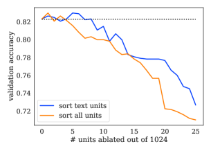
We use milan to obtain descriptions of every residual neuron in the model as well as the first convolutional layer. We identify all neurons whose description contains text, word, or letter. To identify spurious neurons, we first assign each text neuron an independent importance score by removing it from the network and measuring the resulting drop in validation accuracy (with non-adversarial images). We then sort neurons by importance score (with the least important first), and successively ablate them from the model.

Figure 8: ResNet18 accuracy on the adversarial test set as neurons are incrementally ablated. Neurons are sorted by the model’s validation accuracy when that single neuron is ablated, then ablated in that order. When ablating neurons that select for the spurious text, the accuracy improves by 4.9 points. When zeroing arbitrary neurons, accuracy still improves, but by much less.

Results

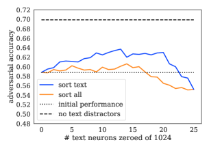
The result of this procedure on adversarial test accuracy is shown in Fig. 8. Training on the spurious data substantially reduces ResNet18’s performance on the adversarial test set: the model achieves 58.8% accuracy, as opposed to 69.9% when tested on non-spurious data. milan identifies 300 text-related convolutional units (out of 1024 examined) in the model, confirming that the model has indeed devoted substantial capacity to identifying text labels in the image. Figure 7c shows an example neurons specifically selective for airline and truck text. By deleting only 13 such neurons, test accuracy is improved by 4.9% (a 12% reduction in overall error rate). This increase cannot be explained by the sorting procedure described above: if instead we sort all neurons according to validation accuracy (orange line), accuracy improves by less than 1%. Thus, while this experiment does not completely eliminate the model’s reliance on text features, it shows that milan’s predictions enable direct editing of networks to partially mitigate sensitivity to spurious feature correlations.

8 Conclusions

We have presented milan, an approach for automatically labeling neurons with natural language descriptions of their behavior. milan selects these descriptions by maximizing pointwise mutual information with image regions in which each neuron is active. These mutual information estimates are in turn produced by a pair of learned models trained on milannotations, a dataset of fine-grained image annotations released with this paper. Descriptions generated by milan surface diverse aspects of model behavior, and can serve as a foundation for numerous analysis, auditing, and editing techniques workflows for users of deep network models.

Impact statement

In contrast to most past work on neuron labeling, milan generates neuron labels using another black-box learned model trained on human annotations of visual concepts. With this increase in expressive power come a number of potential limitations: exemplar-based explanations have known shortcomings (Bolukbasi et al., 2021), human annotations of exemplar sets may be noisy, and the captioning model may itself behave in unexpected ways far outside the training domain. The milannotations dataset was collected with annotator tests to address potential data quality issues, and our evaluation in Section 4 characterizes prediction quality on new networks; we nevertheless emphasize that these descriptions are partial and potentially noisy characterizations of neuron function via their behavior on a fixed-sized set of representative inputs. milan complements, rather than replaces, both formal verification (Dathathri et al., 2020) and careful review of predictions and datasets by expert humans (Gebru et al., 2018; Mitchell et al., 2019).

Appendix A milannotations

(a)

(b)

Figure 9: Screenshots of the Amazon Mechanical Turk forms we used to collect the CaNCAn dataset. (a) The qualification test. Workers are asked to pick the best description for two hand-chosen neurons from a model not included in our corpus. (b) The annotation form. Workers are shown the top-15 highest-activating images for a neuron and asked to describe what is common to them in one sentence.

Figure 10: Example human annotations for neuron exemplars in milannotations, which contains annotations for neurons in seven networks. Each set of images is annotated by three distinct human participants.

We recruited annotators from Amazon Mechanical Turk to describe one neuron at a time given its top-activating images. A screenshot of the template is shown in Figure 9b. Participants were given the instructions:

Instructions: In one sentence, summarize everything shown inside the highlighted regions in the images. They might all show the same thing, or they might show several different things.

In your answer, DO NOT mention that you are describing highlighted regions in images.

Workers were given up to an hour to complete each annotation, but early trials revealed they required about 30 seconds per HIT. We paid workers $0.08 per annotation, which at $9.60 per hour exceeds the United States federal minimum wage.

Model	Dataset	IAA
AlexNet	ImageNet	.25
	Places365	.27
ResNet152	ImageNet	.21
	Places365	.17
BigGAN	ImageNet	.26
	Places365	.24
DINO	ImageNet	.23

Table 4: Average inter-annotator agreement among human annotations, measured in BERTScore. Some models have clearer neuron exemplars than others.

To control for quality, we required workers to pass a short qualification test in which they had to choose the most descriptive caption for two manually chosen neurons from VGG-16 (Simonyan & Zisserman, 2015) trained on ImageNet (not included as part of milannotations). A screenshot of this test is shown in Figure 9a.

Table 4 shows the inter-annotator agreement of neuron annotations for each model, and Table 5 shows some corpus statistics broken down by model and layer. Layers closest to the image (early layers in CNNs and later layers in GANs) are generally described with more adjectives than other layers, while annotations for layers farther from the image include more nouns, perhaps highlighting the low-level perceptual role of the former and the scene- and object-centric behavior of the latter. Layers farther from the image tend to have longer descriptions (e.g. in BigGAN-ImageNet, AlexNet-ImageNet), but this trend is not consistent across all models (e.g. in models trained on Places365, the middle layers have the longest average caption length).

Model	Layer	# Units	# Words	Len.	% Noun	% Adj	% Prep
AlexNet-ImageNet	conv1	64	185	4.8	37.5	24.3	12.2
	conv2	192	384	5.5	37.8	19.4	13.2
	conv3	384	661	5.3	41.0	16.4	13.0
	conv4	256	608	5.5	43.1	11.9	12.5
	conv5	256	693	5.5	46.0	10.2	10.4
AlexNet-Places365	conv1	96	153	4.3	38.4	26.8	12.7
	conv2	256	297	4.8	37.8	26.0	12.7
	conv3	384	412	4.7	40.2	24.8	10.5
	conv4	384	483	4.4	43.7	19.9	10.3
	conv5	256	486	4.1	45.8	17.6	10.6
ResNet152-ImageNet	conv1	64	285	4.7	43.8	11.8	10.3
	layer1	256	653	5.5	43.1	10.5	12.5
	layer2	512	936	5.1	44.0	12.7	12.6
	layer3	1024	1222	4.2	49.6	10.9	11.3
	layer4	2048	1728	4.6	47.8	8.6	7.8
ResNet152-Places365	conv1	64	283	5.2	47.3	11.1	14.6
	layer1	256	633	5.3	46.3	9.4	13.3
	layer2	512	986	5.8	46.0	8.3	13.8
	layer3	1024	1389	4.8	48.2	6.7	12.7
	layer4	2048	1970	5.3	46.3	5.5	11.9
BigGAN-ImageNet	layer0	1536	1147	3.9	52.4	7.8	8.2
	layer1	768	853	3.5	53.0	9.4	8.9
	layer2	768	618	3.2	52.6	12.3	9.5
	layer3	384	495	3.7	49.9	14.3	10.9
	layer4	192	269	3.3	47.9	18.0	13.4
	layer5	96	69	2.6	53.6	22.8	14.6
BigGAN-Places365	layer0	2048	1062	4.2	53.3	5.4	8.3
	layer1	1024	708	3.9	55.0	6.1	11.5
	layer2	1024	410	4.6	52.7	8.1	16.3
	layer3	512	273	5.2	50.4	7.6	15.0
	layer4	256	192	4.6	47.5	9.3	14.9
	layer5	128	123	4.2	46.7	13.5	13.0
DINO-ImageNet	layer0	100	320	4.4	45.7	12.7	4.8
	layer1	100	321	4.2	49.8	9.1	6.8
	layer2	100	285	3.9	53.3	6.2	7.5
	layer3	100	312	3.9	54.4	6.2	7.1
	layer4	100	304	3.9	53.5	4.4	7.0
	layer5	100	287	3.5	55.1	5.5	5.2
	layer6	100	377	3.9	51.3	8.2	5.4
	layer7	100	374	3.8	52.0	6.4	6.2
	layer8	100	330	3.4	53.0	7.0	8.8
	layer9	100	350	3.1	56.1	6.3	9.6
	layer10	100	369	3.9	50.3	9.3	8.2
	layer11	100	294	3.3	52.4	7.5	9.4
Total		20272	4597	4.5	48.7	9.4	10.9

Table 5: Corpus statistics for milannotations descriptions broken down by model and layer. The # Words column reports the number of unique words used across all layer annotations, the Len. column reports the average number of words in each caption for that layer, and the % columns report the percentage of all words across all captions for that layer that are a specific part of speech.

Appendix B milan implementation details

B.1 Implementing $p(d\mid E)$

We build on the Show, Attend, and Tell (SAT) model for describing images (Xu et al., 2015). SAT is designed for describing the high-level content of a single images, so we must make several modifications to support our use case, where our goal is to describe sets of regions in images.

In the original SAT architecture, a single input image $x$ is first converted to visual features by passing it through an encoder network $g$, typically an image classifier pretrained on a large dataset. The output of the last convolutional layer is extracted as a matrix of visual features:

$$v=[v_{1};v_{2};\dots;v_{k}]$$

These visual features are passed to a decoder LSTM whose hidden state is initialized as a function of the mean of the visual features $\overline{v}=1/k\sum_{i}v_{i}$. At each time step, the decoder attends over the features using an additive attention mechanism (Bahdanau et al., 2015), then consumes the attenuated visual features and previous token as input to predict the next token.

Figure 11: Neuron captioning model. Given the set of top-activating images for a neuron and masks for the regions of greatest activation, we extract features maps from each convolutional layer of a pretrained image classifier. We then downsample the masks and use them to pool the features before concatenating them into a single feature vector per image. These feature vectors are used as input to the decoder attention mechanism.

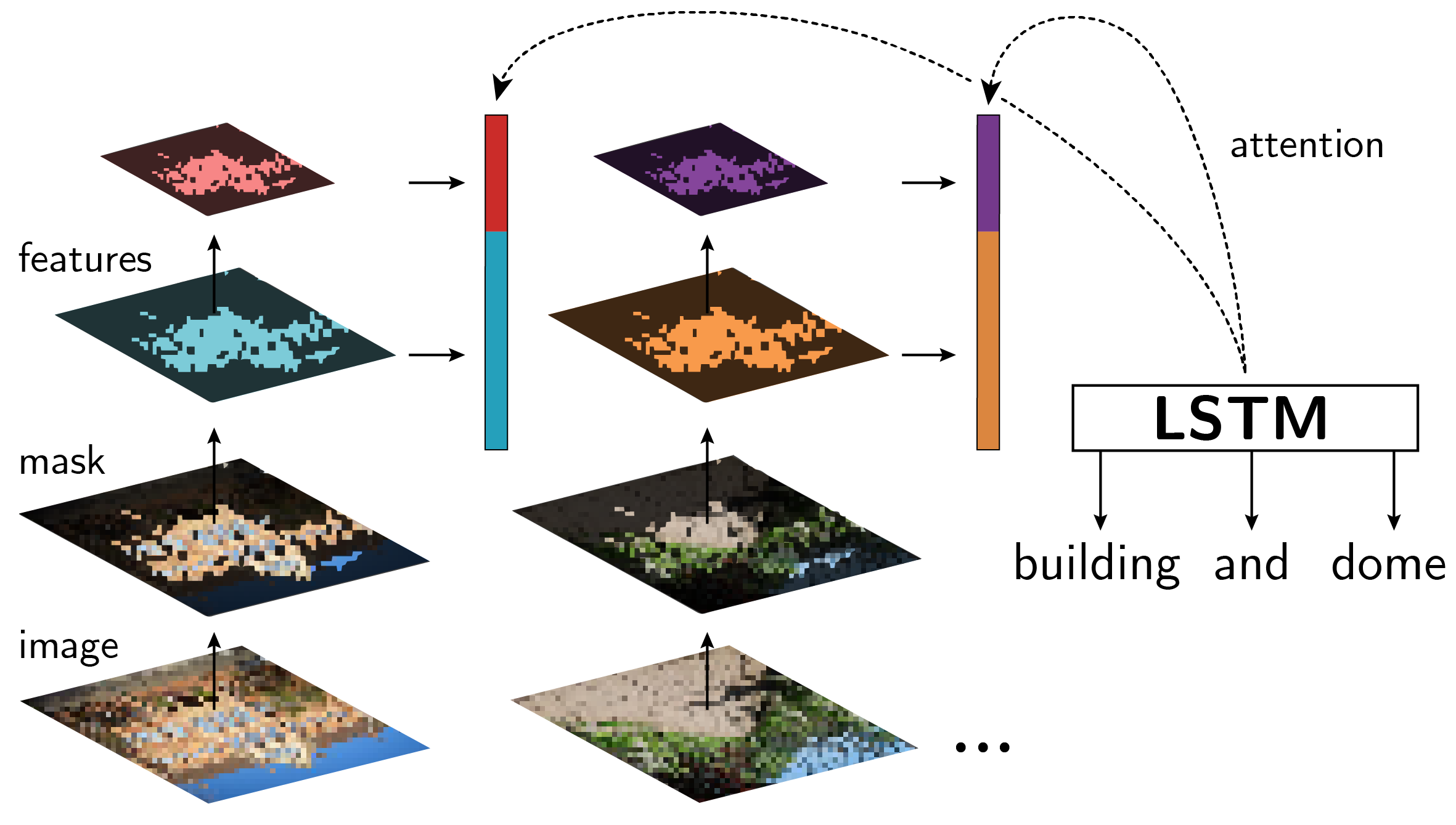
The SAT architecture makes few assumptions about the structure of the visual features. We will take advantage of this generality and modify how $v$ is constructed to support our task, leaving the decoder architecture intact.

Now, instead of a single image $x$, the model inputs are the $k$ top-activating images $x_{j}$ for a neuron as well as a mask $m_{j}$ for each image that highlights the regions of greatest activation. Our task is to describe what the neuron is detecting, based strictly on the highlighted regions of the $x_{j}$. In support of this, the visual features must (1) include information about all $k$ images, (2) encode multiple resolutions of the images to capture both low-level perceptual and high-level scene details about the image, and (3) pay most (but not exclusive) attention to the regions of greatest activation in the image.

Describing sets of images

The $k$ features in SAT correspond to different spatial localities of a single image. In our architecture, each feature $v_{j}$ corresponds to one input image $x_{j}$.

Encoding multiple resolutions

Instead of encoding the image with just the last convolutional layer of $g$, we use pooled convolutional features from every layer. Formally, let $g_{\ell}(x)$ denote the output of layer $\ell$ in the pretrained image encoder with $L$ layers, and let pool denote a pooling function that uses the mask to pool the features (described further below). The feature vector for the $j$th image $x_{j}$ is:

$$v_{j}=\bigg{[}~{}\texttt{pool}(m_{j},g_{1}(x_{j}))~{};~{}\dots~{};~{}\texttt{pool}(m_{i},g_{L}(x_{j}))~{}\bigg{]}$$

Highlighting regions of greatest activation

Each of the top-activating images $x_{j}$ that we hand to our model comes with a mask $m_{j}$ highlighting the image regions of greatest activation. We incorporate these masks into the pooling function pool from above. Specifically, we first downsample the mask $m_{j}$ to the same spatial shape as $g_{\ell}(x_{j})$ using bilinear interpolation, which we denote $\texttt{upsample}(m_{j})$. We then apply the mask to each channel $c$ at layer $\ell$, written $g_{\ell,c}(x_{j})$, via element-wise multiplication ($\odot$) with $\texttt{upsample}(m_{j})$. Finally, we sum spatially along each channel, resulting in a length $c$ vector. Formally:

$$\texttt{pool}_{c}(g_{\ell}(x_{j}))=\mathbbm{1}^{\top}\texttt{vec}(\texttt{upsample}(m_{j})\odot g_{\ell,c}(x_{j}))$$

Each $v_{i}$ is thus a length $\sum_{\ell}C_{\ell}$ vector, where $C_{\ell}$ is the number of channels at layer $\ell$ of $g$.

Throughout our experiments, $g$ is a ResNet101 pretrained for image classification on ImageNet, provided by PyTorch Paszke et al. (2019). We extract visual features from the first convolutional layer and all four residual layers. We do not fine tune any parameters in the encoder. The decoder is a single LSTM cell with an input embedding size of 128 and a hidden size of 512. The attention mechanism linearly maps the current hidden state and all visual feature vectors to size 512 vectors before computing attention weights. We always decode for a maximum of 15 steps. The rest of the decoder is exactly the same as in Xu et al. (2015).

The model is trained to minimize cross entropy on the training set using the AdamW optimizer Loshchilov & Hutter (2019) with a learning rate of 1e-3 and minibatches of size 64. We include the double stochasticity regularization term used by Xu et al. (2015) with $\lambda=1$. We also apply dropout ($p=.5$) to the hidden state before predicting the next word. Across configurations, 10% of the training data is held out and used as a validation set, and training stops when the model’s BLEU score (Papineni et al., 2002) does not improve on this set for 4 epochs, up to a maximum of 100 epochs.

B.2 Implementing $p(d)$

We implement $p(d)$ using a two-layer LSTM language model (Hochreiter & Schmidhuber, 1997). We use an input embedding size of 128 with a hidden state size and cell size of 512. We apply dropout to non-recurrent connections $(p=.5)$ during training and hold out 10% of the training dataset as a validation set and following the same early stopping procedure as in Section B.1, except we stop on validation loss instead of BLEU.

Appendix C Generalization experiment details

Gen.	Train + Test		# Units	# Words	Len.	% Noun	% Adj	% Prep
within netwok	AlexNet–ImageNet		115	100	3.5	45.7	16.4	11.9
	AlexNet–Places		137	46	2.5	49.3	28.7	9.6
	ResNet–ImageNet		390	121	2.8	52.2	23.8	11.7
	ResNet–Places		390	376	4.3	46.5	8.7	10.9
	BigGAN–ImageNet		374	112	2.2	59.8	17.5	10.4
	BigGAN–Places		499	245	3.8	54.2	6.0	9.0
	Train	Test
across arch.	AlexNet	ResNet	7808	326	3.0	46.1	21.0	8.9
	ResNet	AlexNet	2528	275	2.7	48.0	27.1	6.4
	CNNs	ViT	1200	200	2.6	55.0	18.2	13.0
across dataset	ImageNet	Places	10272	271	2.2	58.8	14.0	13.8
	Places	ImageNet	8800	309	3.1	47.8	26.9	7.8
across task	Classifiers	BigGAN	8736	202	2.1	53.0	25.3	6.1
	BigGAN	Classifiers	10336	336	3.2	54.3	14.2	16.8
Total			51585	1002	2.7	51.9	19.8	11.1

Table 6: Statistics for milan-generated descriptions on the held-out neurons from the generalization experiments of Section 4. Columns are the same as in Table 5.

Figure 12: Randomly chosen examples of milan-generated descriptions from the generalization experiments of Section 4.

In each experiment, milan is trained with the hyperparameters described in Appendix B and Section 3.4, with the sole exception being the within-network splits—for these, we increase the early stopping criterion to require 10 epochs of no improvement to account for the training instability caused by the small training set size.

To obtain NetDissect labels, we obtain image exemplars with the same settings as we do for milan, and we obtain segmentations using the full segmentation vocabulary minus the textures.

To obtain Compositional Explanations labels, we search for up to length 3 formulas (comprised of not, and, and or operators) with a beam size of 5 and no length penalty. Image region exemplars and corresponding segmentations come from the ADE20k dataset (Zhou et al., 2019).

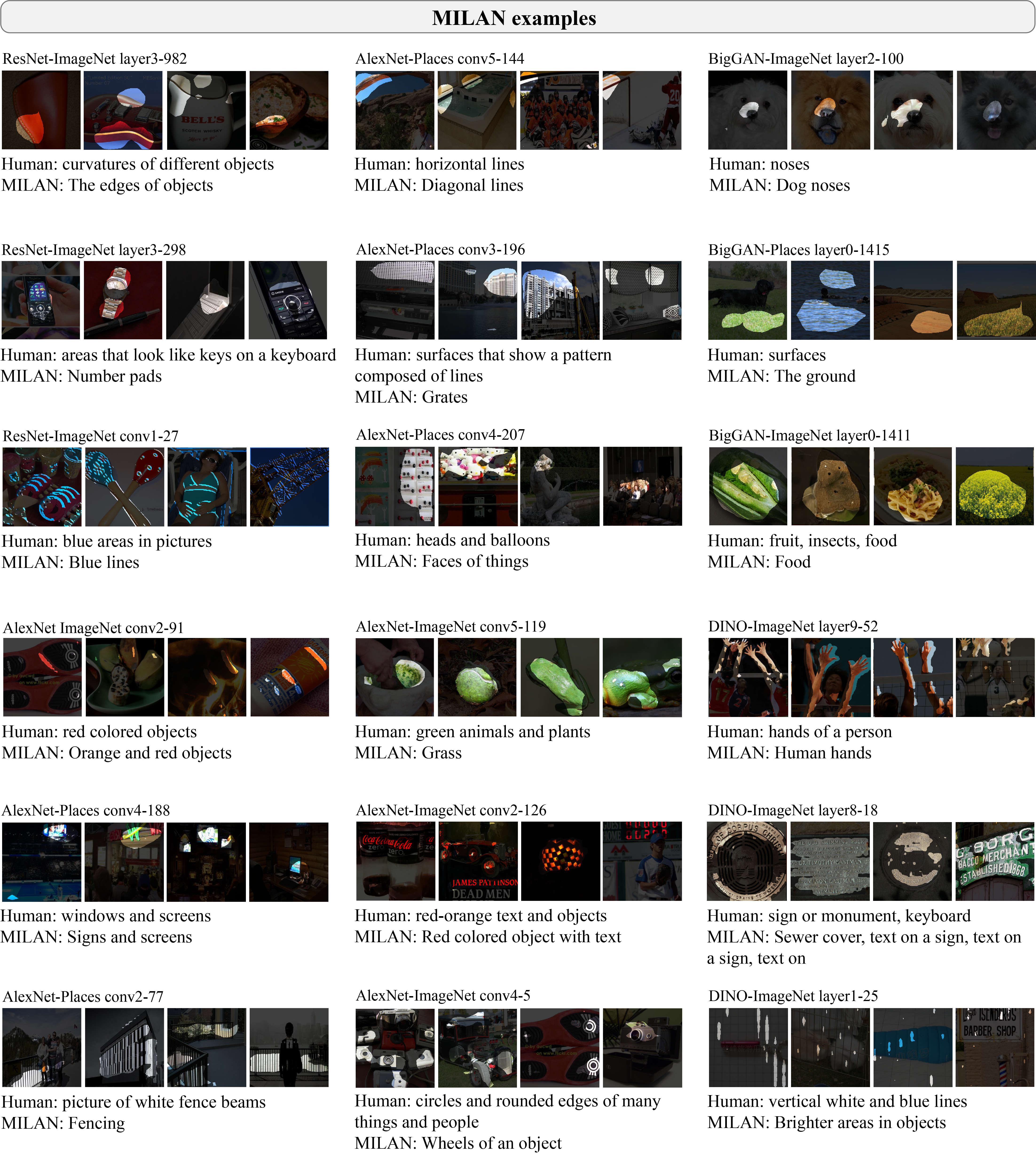
Finally, Table 6 shows statistics for milan descriptions generated on the held out sets from each generalization experiment. Compared to human annotators (Table 5), milan descriptions are on average shorter (2.7 vs. 4.5 tokens), use fewer unique words (1k vs. 4.6k), and contain adjectives twice as often (9.4% vs. 19.8%). Figure 12 contains additional examples, chosen at random.

Appendix D Analysis experiment details

Figure 13: Examples of ablated neurons for each condition Section 5, chosen from among the first 10 ablated.

Figure 14: Cut-and-paste adversarial attacks highlighting non-robust behavior by a neuron that scored high on the max-word-diff criterion of Section 5. (a) milan finds this neuron automatically because the generated description mentions two or more dissimilar concepts: animals and vehicles. The neuron is directly connected to the final fully-connected output layer, and strongly influences amphibian, hermit crab, and jeep predictions according to the connection weights. (b) To construct adversarial inputs, we pick three images from the ImageNet validation set that do not include concepts detected by the neuron. (c) We then select a different set of images to act as distractors that do include the concepts detected by the neuron. (d) By cutting and pasting the central object from the distractor to the original image, the model is fooled into predicting a class label that is completely unrelated to the pasted object: e.g., it predicts amphibian when the military vehicle is pasted.

We obtain the ResNet18 model pretrained on ImageNet from torchvision (Paszke et al., 2019). We obtain neuron descriptions for the same layers that we annotate in ResNet152 (Section 3.3) using the milan hyperparameters described in Section 3.2 and Section 3.4. We obtain part of speech tags, parse trees, and word vectors for each description from spaCy (Honnibal et al., 2020).

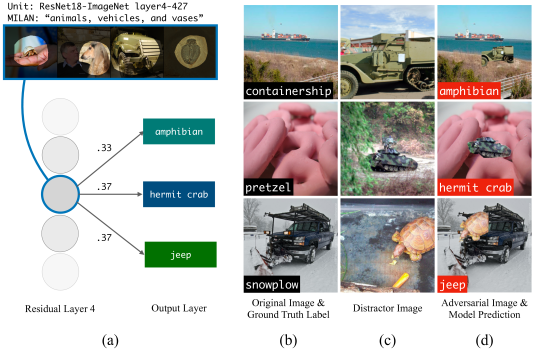
Figure 13 shows examples of neurons that scored high under each criterion (and consequently were among the first ablated in Fig. 5). Note that these examples include some failure cases of milan: for example, in the # verbs example, milan incorrectly categorizes all brass instruments as flutes; and in the # adjectives example, the description is disfluent. Nevertheless, these examples confirm our intuitions about the kinds of neurons selected for by each scoring criterion, as described in Section 5.

We hypothesized in Section 5 that neurons scoring high on the max-word-diff criterion correspond to non-robust behavior by the model. Figure 14 provides some evidence for this hypothesis: we construct cut-and-paste adversarial inputs in the style of Mu & Andreas (2020). Specifically, we look at the example max-word-diff neuron shown in Figure 13, crudely copy and paste one of the objects mentioned in its description (e.g., a vehicle-related object like a half track), and show that this can cause the model to predict one of the other concepts in the description (e.g., an animal-related class like amphibian).

Appendix E Editing experiment details

Hyperparameters

We train a randomly initialized ResNet18 on the spurious training dataset for a maximum of 100 epochs with a learning rate of 1e-4 and a minibatch size of 128. We annotate the same convolutional and residual units we did for ResNet152 in Section 3.3. We stop training when validation loss does not improve for 4 epochs.

How many neurons should we remove?

In practice, we cannot incrementally test our model on an adversarial set. So how do we decide on the number of neurons to zero? One option is to look solely at validation accuracy. Figure 15 recreates Figure 8 with accuracy on the held out validation set (which is distributed like the training dataset) instead of accuracy on the adversarial test set. The accuracy starts peaks and starts decreasing earlier than in Fig. 8, but if we were to choose the number to be the largest before validation accuracy permanently decreases, we would choose 8 neurons, which would still result in a 3.1% increase in adversarial accuracy.

Figure 15: Same as Fig. 8, but shows accuracy on the validation dataset, which is distributed identically to the training dataset. Dotted line denotes initial accuracy.

References

- Andreas & Klein (2017) Jacob Andreas and Dan Klein. Analogs of linguistic structure in deep representations. In Proceedings of the 2017 Conference on Empirical Methods in Natural Language Processing, pp. 2893–2897, Copenhagen, Denmark, September 2017. Association for Computational Linguistics. doi: 10.18653/v1/D17-1311. URL https://www.aclweb.org/anthology/D17-1311.
- Andreas et al. (2017) Jacob Andreas, Anca D Dragan, and Dan Klein. Translating neuralese. In ACL (1), 2017.
- Bahdanau et al. (2015) Dzmitry Bahdanau, Kyung Hyun Cho, and Yoshua Bengio. Neural machine translation by jointly learning to align and translate. In ICLR, January 2015.
- Bau et al. (2018) Anthony Bau, Yonatan Belinkov, Hassan Sajjad, Nadir Durrani, Fahim Dalvi, and James Glass. Identifying and controlling important neurons in neural machine translation. In International Conference on Learning Representations, 2018.
- Bau et al. (2017) David Bau, Bolei Zhou, Aditya Khosla, Aude Oliva, and Antonio Torralba. Network dissection: Quantifying interpretability of deep visual representations. In Computer Vision and Pattern Recognition (CVPR), 2017.
- Bau et al. (2019) David Bau, Jun-Yan Zhu, Hendrik Strobelt, Bolei Zhou, Joshua B Tenenbaum, William T Freeman, and Antonio Torralba. Gan dissection: Visualizing and understanding generative adversarial networks. In International Conference on Learning Representations (ICLR), 2019.
- Bau et al. (2020) David Bau, Jun-Yan Zhu, Hendrik Strobelt, Agata Lapedriza, Bolei Zhou, and Antonio Torralba. Understanding the role of individual units in a deep neural network. Proceedings of the National Academy of Sciences (PNAS), 2020.
- Bolukbasi et al. (2021) Tolga Bolukbasi, Adam Pearce, Ann Yuan, Andy Coenen, Emily Reif, Fernanda Viégas, and Martin Wattenberg. An interpretability illusion for bert. arXiv preprint arXiv:2104.07143, 2021.
- Brock et al. (2018) Andrew Brock, Jeff Donahue, and Karen Simonyan. Large scale gan training for high fidelity natural image synthesis. In International Conference on Learning Representations, 2018.
- Camburu et al. (2018) Oana-Maria Camburu, Tim Rocktäschel, Thomas Lukasiewicz, and Phil Blunsom. e-snli: Natural language inference with natural language explanations. arXiv preprint arXiv:1812.01193, 2018.
- Cammarata et al. (2021) Nick Cammarata, Gabriel Goh, Shan Carter, Chelsea Voss, Ludwig Schubert, and Chris Olah. Curve circuits. Distill, 6(1):e00024–006, 2021.
- Caron et al. (2021) Mathilde Caron, Hugo Touvron, Ishan Misra, Hervé Jégou, Julien Mairal, Piotr Bojanowski, and Armand Joulin. Emerging properties in self-supervised vision transformers. In Proceedings of the International Conference on Computer Vision (ICCV), 2021.
- Chen & He (2020) Xinlei Chen and Kaiming He. Exploring simple siamese representation learning, 2020.
- Dalvi et al. (2019) Fahim Dalvi, Nadir Durrani, Hassan Sajjad, Yonatan Belinkov, Anthony Bau, and James Glass. What is one grain of sand in the desert? analyzing individual neurons in deep nlp models. In Proceedings of AAAI, 2019.
- Dathathri et al. (2020) Sumanth Dathathri, Krishnamurthy Dvijotham, Alexey Kurakin, Aditi Raghunathan, Jonathan Uesato, Rudy Bunel, Shreya Shankar, Jacob Steinhardt, Ian Goodfellow, Percy Liang, et al. Enabling certification of verification-agnostic networks via memory-efficient semidefinite programming. In Neural Information Processing Systems (NeurIPS), 2020.
- Deng et al. (2009) Jia Deng, Wei Dong, Richard Socher, Li-Jia Li, Kai Li, and Li Fei-Fei. Imagenet: A large-scale hierarchical image database. In Computer Vision and Pattern Recognition (CVPR), 2009.
- Donahue et al. (2015) Jeffrey Donahue, Lisa Anne Hendricks, Sergio Guadarrama, Marcus Rohrbach, Subhashini Venugopalan, Kate Saenko, and Trevor Darrell. Long-term recurrent convolutional networks for visual recognition and description. In Proceedings of the IEEE conference on computer vision and pattern recognition, pp. 2625–2634, 2015.
- Dosovitskiy et al. (2021) Alexey Dosovitskiy, Lucas Beyer, Alexander Kolesnikov, Dirk Weissenborn, Xiaohua Zhai, Thomas Unterthiner, Mostafa Dehghani, Matthias Minderer, Georg Heigold, Sylvain Gelly, et al. An image is worth 16x16 words: Transformers for image recognition at scale. In International Conference on Learning Representations (ICLR), 2021.
- Erhan et al. (2009) Dumitru Erhan, Yoshua Bengio, Aaron Courville, and Pascal Vincent. Visualizing higher-layer features of a deep network. 2009.
- Gebru et al. (2018) Timnit Gebru, Jamie Morgenstern, Briana Vecchione, Jennifer Wortman Vaughan, Hanna Wallach, Hal Daumé III, and Kate Crawford. Datasheets for datasets. arXiv preprint arXiv:1803.09010, 2018.
- Girshick et al. (2014) Ross Girshick, Jeff Donahue, Trevor Darrell, and Jitendra Malik. Rich feature hierarchies for accurate object detection and semantic segmentation. In computer vision and pattern recognition (CVPR), pp. 580–587, 2014.
- Goh et al. (2021) Gabriel Goh, Nick Cammarata, Chelsea Voss, Shan Carter, Michael Petrov, Ludwig Schubert, Alec Radford, and Chris Olah. Multimodal neurons in artificial neural networks. Distill, 2021.
- Grill et al. (2020) Jean-Bastien Grill, Florian Strub, Florent Altché, Corentin Tallec, Pierre H. Richemond, Elena Buchatskaya, Carl Doersch, Bernardo Avila Pires, Zhaohan Daniel Guo, Mohammad Gheshlaghi Azar, Bilal Piot, Koray Kavukcuoglu, Rémi Munos, and Michal Valko. Bootstrap your own latent: A new approach to self-supervised learning, 2020.
- He et al. (2015) Kaiming He, Xiangyu Zhang, Shaoqing Ren, and Jian Sun. Deep residual learning for image recognition, 2015.
- Hendricks et al. (2016) Lisa Anne Hendricks, Zeynep Akata, Marcus Rohrbach, Jeff Donahue, Bernt Schiele, and Trevor Darrell. Generating visual explanations. In European conference on computer vision, pp. 3–19. Springer, 2016.
- Hendricks et al. (2018) Lisa Anne Hendricks, Ronghang Hu, Trevor Darrell, and Zeynep Akata. Grounding visual explanations. In Proceedings of the European Conference on Computer Vision (ECCV), pp. 264–279, 2018.
- Hochreiter & Schmidhuber (1997) Sepp Hochreiter and Jürgen Schmidhuber. Long short-term memory. In Neural computation, 1997.
- Honnibal et al. (2020) Matthew Honnibal, Ines Montani, Sofie Van Landeghem, and Adriane Boyd. spaCy: Industrial-strength Natural Language Processing in Python, 2020. URL https://doi.org/10.5281/zenodo.1212303.
- Jaccard (1912) Paul Jaccard. The distribution of the flora in the alpine zone. New Phytologist, 11(2):37–50, 1912.
- Karpathy et al. (2015) Andrej Karpathy, Justin Johnson, and Li Fei-Fei. Visualizing and understanding recurrent networks. arXiv preprint arXiv:1506.02078, 2015.
- Kim et al. (2018) Been Kim, Martin Wattenberg, Justin Gilmer, Carrie Cai, James Wexler, Fernanda Viegas, et al. Interpretability beyond feature attribution: Quantitative testing with concept activation vectors (tcav). In International conference on machine learning (ICML), 2018.
- Krizhevsky et al. (2012) Alex Krizhevsky, Ilya Sutskever, and Geoffrey E Hinton. Imagenet classification with deep convolutional neural networks. In Advances in Neural Information Processing Systems (NeurIPS), 2012.
- Laina et al. (2020) Iro Laina, Ruth C. Fong, and Andrea Vedaldi. Quantifying learnability and describability of visual concepts emerging in representation learning. Advances in Neural Information Processing Systems, 2020-December, 2020. ISSN 1049-5258. Funding Information: We would like to thank Yuki Asano and Christian Rupprecht for helpful discussions and for their feedback on this work. We are also grateful for the EPSRC programme grant Seebibyte EP/M013774/1 (I.L.), ERC starting grant IDIU 638009 (I.L), and Open Philanthropy Project (R.F.). Publisher Copyright: © 2020 Neural information processing systems foundation. All rights reserved.; 34th Conference on Neural Information Processing Systems, NeurIPS 2020 ; Conference date: 06-12-2020 Through 12-12-2020.
- Lin et al. (2014) Tsung-Yi Lin, Michael Maire, Serge Belongie, James Hays, Pietro Perona, Deva Ramanan, Piotr Dollár, and C. Lawrence Zitnick. Microsoft coco: Common objects in context. In David Fleet, Tomas Pajdla, Bernt Schiele, and Tinne Tuytelaars (eds.), Computer Vision – ECCV 2014, pp. 740–755, Cham, 2014. Springer International Publishing. ISBN 978-3-319-10602-1.
- Loshchilov & Hutter (2019) Ilya Loshchilov and Frank Hutter. Decoupled weight decay regularization. In ICLR, 2019.
- Mahendran & Vedaldi (2015) Aravindh Mahendran and Andrea Vedaldi. Understanding deep image representations by inverting them. In computer vision and pattern recognition (CVPR), 2015.
- Mitchell et al. (2019) Margaret Mitchell, Simone Wu, Andrew Zaldivar, Parker Barnes, Lucy Vasserman, Ben Hutchinson, Elena Spitzer, Inioluwa Deborah Raji, and Timnit Gebru. Model cards for model reporting. In Proceedings of the conference on fairness, accountability, and transparency, pp. 220–229, 2019.
- Morcos et al. (2018) Ari S Morcos, David GT Barrett, Neil C Rabinowitz, and Matthew Botvinick. On the importance of single directions for generalization. In International Conference on Learning Representations (ICLR), 2018.
- Mu & Andreas (2020) Jesse Mu and Jacob Andreas. Compositional explanations of neurons. In Advances in Neural Information Processing Systems, 2020.
- Narang et al. (2020) Sharan Narang, Colin Raffel, Katherine Lee, Adam Roberts, Noah Fiedel, and Karishma Malkan. WT5?! Training text-to-text models to explain their predictions. arXiv preprint arXiv:2004.14546, 2020.
- Olah et al. (2017) Chris Olah, Alexander Mordvintsev, and Ludwig Schubert. Feature visualization. In Distill, 2017.
- Olah et al. (2018) Chris Olah, Arvind Satyanarayan, Ian Johnson, Shan Carter, Ludwig Schubert, Katherine Ye, and Alexander Mordvintsev. The building blocks of interpretability. In Distill, 2018.
- Papineni et al. (2002) Kishore Papineni, Salim Roukos, Todd Ward, and Wei-Jing Zhu. Bleu: a method for automatic evaluation of machine translation. In Proceedings of the 40th annual meeting of the Association for Computational Linguistics, pp. 311–318, 2002.
- Park et al. (2018) Dong Huk Park, Lisa Anne Hendricks, Zeynep Akata, Anna Rohrbach, Bernt Schiele, Trevor Darrell, and Marcus Rohrbach. Multimodal explanations: Justifying decisions and pointing to the evidence. In Proceedings of the IEEE Conference on Computer Vision and Pattern Recognition, pp. 8779–8788, 2018.
- Paszke et al. (2019) Adam Paszke, Sam Gross, Francisco Massa, Adam Lerer, James Bradbury, Gregory Chanan, Trevor Killeen, Zeming Lin, Natalia Gimelshein, Luca Antiga, Alban Desmaison, Andreas Kopf, Edward Yang, Zachary DeVito, Martin Raison, Alykhan Tejani, Sasank Chilamkurthy, Benoit Steiner, Lu Fang, Junjie Bai, and Soumith Chintala. Pytorch: An imperative style, high-performance deep learning library. In H. Wallach, H. Larochelle, A. Beygelzimer, F. d'Alché-Buc, E. Fox, and R. Garnett (eds.), Advances in Neural Information Processing Systems 32, pp. 8024–8035. Curran Associates, Inc., 2019. URL http://papers.neurips.cc/paper/9015-pytorch-an-imperative-style-high-performance-deep-learning-library.pdf.
- Preuer et al. (2019) Kristina Preuer, Günter Klambauer, Friedrich Rippmann, Sepp Hochreiter, and Thomas Unterthiner. Interpretable deep learning in drug discovery. In Explainable AI: Interpreting, Explaining and Visualizing Deep Learning, pp. 331–345. Springer, 2019.
- Radford et al. (2017) Alec Radford, Rafal Jozefowicz, and Ilya Sutskever. Learning to generate reviews and discovering sentiment. arXiv preprint arXiv:1704.01444, 2017.
- Rajani et al. (2019) Nazneen Fatema Rajani, Bryan McCann, Caiming Xiong, and Richard Socher. Explain yourself! leveraging language models for commonsense reasoning. arXiv preprint arXiv:1906.02361, 2019.
- Rashtchian et al. (2010) Cyrus Rashtchian, Peter Young, Micah Hodosh, and Julia Hockenmaier. Collecting image annotations using amazon’s mechanical turk. In Proceedings of the NAACL HLT 2010 Workshop on Creating Speech and Language Data with Amazon’s Mechanical Turk, pp. 139–147, 2010.
- Schwettmann et al. (2021) Sarah Schwettmann, Evan Hernandez, David Bau, Samuel Klein, Jacob Andreas, and Antonio Torralba. Toward a visual concept vocabulary for gan latent space. International Conference on Computer Vision, 2021.
- Sharma et al. (2018) Piyush Sharma, Nan Ding, Sebastian Goodman, and Radu Soricut. Conceptual captions: A cleaned, hypernymed, image alt-text dataset for automatic image captioning. In Proceedings of ACL, 2018.
- Simonyan & Zisserman (2015) Karen Simonyan and Andrew Zisserman. Very deep convolutional networks for large-scale image recognition. In International Conference on Learning Representations (ICLR), 2015.
- Storkey (2009) Amos Storkey. When training and test sets are different: characterizing learning transfer. Dataset shift in machine learning, 30:3–28, 2009.
- Vaughan & Wallach (2020) Jennifer Wortman Vaughan and Hanna Wallach. A human-centered agenda for intelligible machine learning. Machines We Trust: Getting Along with Artificial Intelligence, 2020.
- Wang et al. (2020) Zeyu Wang, Berthy Feng, Karthik Narasimhan, and Olga Russakovsky. Towards unique and informative captioning of images. In European Conference on Computer Vision (ECCV), 2020.
- Xiao et al. (2020) Kai Xiao, Logan Engstrom, Andrew Ilyas, and Aleksander Madry. Noise or signal: The role of image backgrounds in object recognition. arXiv preprint arXiv:2006.09994, 2020.
- Xu et al. (2015) Kelvin Xu, Jimmy Lei Ba, Ryan Kiros, Kyunghyun Cho, Aaron Courville, Ruslan Salakhutdinov, Richard S. Zemel, and Yoshua Bengio. Show, attend and tell: Neural image caption generation with visual attention. In Proceedings of the 32nd International Conference on International Conference on Machine Learning - Volume 37, ICML’15, pp. 2048–2057. JMLR.org, 2015.
- Yang et al. (2021) Kaiyu Yang, Jacqueline Yau, Li Fei-Fei, Jia Deng, and Olga Russakovsky. A study of face obfuscation in imagenet. arXiv preprint arXiv:2103.06191, 2021.
- Zaidan & Eisner (2008) Omar Zaidan and Jason Eisner. Modeling annotators: A generative approach to learning from annotator rationales. In Proceedings of the 2008 conference on Empirical methods in natural language processing, pp. 31–40, 2008.
- Zeiler & Fergus (2014) Matthew D Zeiler and Rob Fergus. Visualizing and understanding convolutional networks. ECCV, 2014.
- Zellers et al. (2019) Rowan Zellers, Yonatan Bisk, Ali Farhadi, and Yejin Choi. From recognition to cognition: Visual commonsense reasoning. In Proceedings of the IEEE/CVF Conference on Computer Vision and Pattern Recognition, pp. 6720–6731, 2019.
- Zhang et al. (2020) Tianyi Zhang, Varsha Kishore, Felix Wu, Kilian Q. Weinberger, and Yoav Artzi. Bertscore: Evaluating text generation with bert. In International Conference on Learning Representations, 2020. URL https://openreview.net/forum?id=SkeHuCVFDr.
- Zhou et al. (2017) Bolei Zhou, Agata Lapedriza, Aditya Khosla, Aude Oliva, and Antonio Torralba. Places: A 10 million image database for scene recognition. IEEE transactions on pattern analysis and machine intelligence, 2017.
- Zhou et al. (2019) Bolei Zhou, Hang Zhao, Xavier Puig, Tete Xiao, Sanja Fidler, Adela Barriuso, and Antonio Torralba. Semantic understanding of scenes through the ade20k dataset. International Journal of Computer Vision, 127(3):302–321, 2019.