On the behavior of multidimensional radially symmetric solutions of the repulsive Euler-Poisson equations

Abstract.

It is proved that the radially symmetric solutions of the repulsive Euler-Poisson equations with a non-zero background, corresponding to cold plasma oscillations blow up in many spatial dimensions except for ${\bf d}=4$ for almost all initial data. The initial data, for which the solution may not blow up, correspond to simple waves. Moreover, if a solution is globally smooth in time, then it is either affine or tends to affine as $t\to\infty$.

1. Introduction

In this paper, we study a version of the repulsive Euler-Poisson equations

(1) $$\displaystyle{\partial n\over\partial t}+\mbox{div}\,(n{\bf V})=0,\quad\displaystyle{\partial{\bf V}\over\partial t}+\left({\bf V}\cdot\nabla\right){\bf V}=\,k\,\nabla\Phi,\quad\Delta\Phi=n-n_{0},$$

where the solution components, the scalar functions $n$ (density), $\Phi$ (force potential), and the vector ${\bf V}$ (velocity) depend on the time $t$ and the point $x\in{\mathbb{R}}^{\bf d}$, ${\bf d}\geq 1$, $n_{0}>0$ is the density background. Positive or negative value of the constant $k$ corresponds to the repulsive and attractive force, respectively.

The Euler-Poisson equations arise in many applications, see [11] for references, but for us they are of interest primarily in the context of cold plasma oscillations, where $k=1$. At present, much attention is paid to the study of cold plasma in connection with the possibility of accelerating electrons in the wake wave of a powerful laser pulse [13]; nevertheless, there are very few theoretical results in this area.

The equations of hydrodynamics of “cold” or electron plasma in the non-relativistic approximation in dimensionless quantities have the form (see, e.g., [1], [8])

(2) $$\displaystyle{\partial n\over\partial t}+\mbox{div}\,(n{\bf V})=0,\quad\displaystyle{\partial{\bf V}\over\partial t}+\left({\bf V}\cdot\nabla\right){\bf V}=\,-{\bf E}-\left[{\bf V}\times{\bf B}\right],$$

(3) $$\frac{\partial{\bf E}}{\partial t}=n{\bf V}+{\rm rot}\,{\bf B},\qquad\frac{\partial{\bf B}}{\partial t}=-{\rm rot}\,{\bf E},\qquad\mbox{div}\,{\bf B}=0,$$

$n$ and ${\bf V}=(V_{1},V_{2},V_{3})$ are the density and velocity of electrons, ${\bf E}=(E_{1},E_{2},E_{3})$ and ${\bf B}=(B_{1},B_{2},B_{3})$ are vectors of electric and magnetic fields. All components of solution depends on $t\in{\mathbb{R}}_{+}$ and $x\in{\mathbb{R}}^{3}$.

It is commonly known that the plasma oscillations described by (2), (3), tend to break. Mathematically, the breaking process means a blow-up of the solution, and the appearance of a delta-shape singularity of the electron density [6], see also [5] and references therein for numerical examples illustrating the behavior of solution on the stage of the blow-up. Among the main interests of physicists is the study of the possibility of the existence of a smooth solution for as long as possible.

System (2) – (3) has an important class of solutions depending only on the radius-vector of point $r=\sqrt{x_{1}^{2}+x_{2}^{2}+x_{3}^{2}}$, i.e.

(4) $${\bf V}=F(t,r){\bf r},\quad{\bf E}=G(t,r){\bf r},\quad{\bf B}=Q(t,r){\bf r},\quad n=n(t,r),$$

where ${\bf r}=(x_{1},x_{2},x_{3})$.

Since ${\rm div}{\bf B}=3Q(t,r)+r(Q(t,r))_{r},$ then the condition ${\rm div}{\bf B}=0$ implies $Q(t,r)=\tilde{Q}(t)r^{-3}$, therefore a bounded in the origin solution exists if and only if ${\bf B}\equiv 0.$ In its turn, it implies ${\rm rot}\,{\bf E}=0$. From the first equations of (2) and (3) under the assumption that the solution is sufficiently smooth and that the steady-state density $n_{0}$ is equal to 1, we get

(5) $$n=1-\mbox{div}\,{\bf E},$$

therefore $n$ can be removed from the system. Thus, the resulting system is

(6) $$\displaystyle{\partial{\bf V}\over\partial t}+\left({\bf V}\cdot\nabla\right){\bf V}=\,-{\bf E},\quad\frac{\partial{\bf E}}{\partial t}+{\bf V}\mbox{div}\,{\bf E}={\bf V}.$$

If we introduce the potential $\Phi$ such that $\nabla\Phi=-{\bf E}$, we can rewrite system (5), (6) as the Euler-Poisson equations (1) with $n_{0}=1$.

Note that system (6) can be considered in any space dimensions ${\bf d}$ (non necessarily ${\bf d}=3$, as in the initial setting). In what follows, we deal with just this case.

Consider the initial data

(7) $$({\bf V},{\bf E})|_{t=0}=(F_{0}(r){\bf r},G_{0}(r){\bf r}),\quad(F_{0}(r),G_{0}(r))\in C^{2}(\bar{\mathbb{R}}_{+}),$$

where ${\bf r}=(x_{1},\dots,x_{\bf d}),\quad r=|{\bf r}|,$ with the physically natural condition $n|_{t=0}>0$.

We call a solution of (6), (7) smooth for $t\in[0,t_{*})$, $t_{*}\leq\infty$, if the functions $F$ and $G$ in (4) belong to the class $C^{1}([0,t_{*})\times\bar{\mathbb{R}}_{+})$. The blow-up of solution implies that the derivatives of solution tends to infinity as $t\to t_{*}<\infty$.

Definition 1.

Solution $({\bf V},{\bf E})$ to system (6) is called an affine solution if it has the form ${\bf V}=\mathfrak{V}(t){\bf r}$, ${\bf E}=\mathfrak{E}(t){\bf r}$, where $\mathfrak{V}$ and $\mathfrak{E}$ are $({\bf d}\times{\bf d})$ matrices.

Definition 2.

Solution $({\bf V},{\bf E})$ to system (6) is called a simple wave if it has the form ${\bf V}=F(t,r){\bf r}$, ${\bf E}=G(t,r){\bf r}$, where $F(t,r)$ and $G(t,r)$ are functionally dependent.

The main result of this paper is the following:

Theorem 1.

The solution of the Cauchy problem (6), (7) for ${\bf d}\geq 2$, ${\bf d}\neq 4$, blows up in a finite time for all initial data, possibly except for the data, corresponding to simple waves. If the solution is globally smooth in time, then it is either affine or tends in the $C^{1}$-norm on each compact subset of the half-axis $[0,\infty)$ to an affine solution as $t\to\infty$.

Theorem 1 can be reformulated in the terms of the Euler-Poisson equations (1).

The results are obtained analytically for small deviations of the trivial steady state and partly thanks to numerical considerations for arbitrary initial data.

The meaning of Theorem 1 is that in spaces of higher dimensions (except for ${\bf d}=4$) there cannot be a non-trivial solution of the Euler-Poisson equations, globally smooth in time, for practically all initial data. In other words, if we want to get a globally smooth solution, we must choose the initial data in a very narrow class of”simple waves, for which one component the solution depends on another. Such a class of solutions cannot be realized as a perturbation of a stationary state with a compact support (see Sec.6), which makes them unpromising both from the point of view of physical applications and from the point of view of a computational experiment.

Note that many results can be obtained in a more convenient way for the Euler-Poisson equations written as (6), this applies, in particular, to equations with linear damping, cf. [18] and [2].

An important contribution to the study of critical phenomena of solutions of the repulsive Euler-Poisson equations was made in [11], where, in particular, radially symmetric solutions in a space of many dimensions are studied. In [20] a critical threshold in the terms of the initial data was obtained for this case. However, the background value of the density was taken as zero in all these studies. In our case, a nonzero background density naturally arises, which leads to the appearance of oscillations and radically changes the research technique and the behavior of the solution. Let us note [19], which contains some progress in this case.

Note that the behavior of the solution changes significantly in the case attractive case $k<0$ , we refer to [3], where conditions for the existence of a globally smooth solution in terms of initial data for zero and non-zero backgrounds are obtained. See also [2] for recent interesting results concerning critical thresholds in Euler-Poisson systems in different settings.

2. Explicit solutions along characteristics

First of all, we notice that (4) and (6) imply that $F$ and $G$ satisfy the following Cauchy problem:

(8) $$\displaystyle{\partial G\over\partial t}+Fr\displaystyle{\partial G\over\partial r}=F-{\bf d}FG,\quad\displaystyle{\partial F\over\partial t}+Fr\displaystyle{\partial F\over\partial r}=-F^{2}-G,$$

(9) $$(F(0,r),G(0,r))=(F_{0}(r),G_{0}(r)),\quad(F_{0}(r),G_{0}(r))\in C^{2}(\bar{\mathbb{R}}_{+}).$$

Along the characteristic

(10) $$\dot{r}=Fr,$$

starting from the point $r_{0}\in[0,\infty)$ system (8) takes the form

(11) $$\dot{G}=F-{\bf d}FG,\qquad\dot{F}=-F^{2}-G.$$

On the phase plane $(G,F)$ system (11) implies one equation

$$\frac{1}{2}\displaystyle{dF^{2}\over dG}=-\frac{F^{2}+G}{1-{\bf d}G},$$

which is linear with respect to $F^{2}$ and can be explicitly integrated. Indeed, we have for ${\bf d}=2$

(12) $$2F^{2}=(2G-1)\ln|1-2G|+C_{2}(2G-1)-1,$$

$$C_{2}=\frac{1+2F^{2}(0,r_{0})}{2G(0,r_{0})-1}-\ln|1-2G(0,r_{0})|,$$

for ${\bf d}=1$ and ${\bf d}\geq 3$

(13) $$F^{2}=\frac{2G-1}{{\bf d}-2}+C_{\bf d}|1-{\bf d}G|^{\frac{2}{{\bf d}}},\quad C_{\bf d}=\frac{1-2G(0,r_{0})+({\bf d}-2)F^{2}(0,r_{0})}{({\bf d}-2)|1-{\bf d}G(0,r_{0})|^{\frac{2}{{\bf d}}}}.$$

Lemma 1.

The condition $n>0$ implies $G<\frac{1}{{\bf d}}$ provided $G(t,r)\in C^{1}([0,t_{*})\times\bar{\mathbb{R}})$, $t_{*}\leq\infty$.

Proof.

From the first equation (11) and (10) we have

(14) $$1-{\bf d}\,G={\rm const}\,r^{-{\bf d}},$$

therefore the sign of $1-{\bf d}\,G(r(t))$ coincides with the sign of $1-{\bf d}G(0,r_{0})$, this means that on the phase plane $(G,F)$ of the system (11) the motions on the half-planes $G<\frac{1}{{\bf d}}$ and $G>\frac{1}{{\bf d}}$ are separated.

Since (5) implies $\mbox{div}\,{\bf E}={\bf d}\,G+G_{r}r<1$, then at the point $r=0$ the condition $G<\frac{1}{{\bf d}}$ follows from (5) directly. Further, on the phase plane $(G,F)$ there is only one equilibrium, the origin. Therefore, in the half-plane $G>\frac{1}{{\bf d}}$ no bounded trajectory exists. If in some point $r_{0}>0$ initially ${\bf d}\,G(0,r_{0})>1$, then $G(r(t))\to+\infty$ and $r(t)\to 0$ as $t\to t_{*}>0$ (see (14)), and we obtain a contradiction with property $n>0$. $\Box$

Lemma 2.

For ${\bf d}\geq 2$ the functions $F$ and $G$ are bounded if and only if $G_{0}(r)<\frac{1}{{\bf d}}$.

Proof.

If $G(0,r_{0})<\frac{1}{{\bf d}}$, $r_{0}\in\bar{\mathbb{R}}$, then the phase trajectories of (11) are in the half-plane $G<\frac{1}{{\bf d}}$ (Lemma 1). In this half-plane the leading term in the right hand side of (12) is $(2\,G-1)\ln|1-2\,G|$, and the leading term in the right hand side of (13) is $\frac{2\,G-1}{{\bf d}-2}$. Therefore $F$ and $G$ are bounded for any $t>0$. $\Box$

Note that the situation is different for ${\bf d}=1$, where the phase trajectory is bounded not for all $G<\frac{1}{{\bf d}}=1$. Indeed, the leading term as $G\to-\infty$ in the right hand side of (13) is $C_{1}(1-G)^{2}$, $F$ and $G$ can be bounded if only if $\displaystyle C_{1}=\frac{F^{2}(0)+2G(0)-1}{(1-G(0))^{2}}<0$ for every $r_{0}$. The 1D case is completely analyzed in [17].

Our considerations also imply

Lemma 3.

Let ${\bf d}\geq 2$. Then along every characteristic curve starting from $r_{0}\in\bar{\mathbb{R}}_{+}$ the functions $F(t)$ and $G(t)$, solution of (11), are periodic with the period

(15) $$T=2\int\limits_{G_{-}}^{G_{+}}\frac{d\eta}{(1-{\bf d}\,\eta)F(\eta)},$$

$F$ is given as (12) or (13), $G_{-}<0$ and $G_{+}>0$ are the lesser and greater roots of the equation $F(G)=0$. Moreover, $\int\limits_{0}^{T}F(\tau)\,d\tau=0$.

The last property follows from the fact that the phase curve of (11) is symmetric with respect to the axis $F=0$.

The following lemma helps us to study the properties of the period $T$ depending on ${\bf d}$.

Lemma 4.

The period of revolution of the phase curve of equation (11) depends on ${\bf d}$ and the starting point of trajectory, except for ${\bf d}=1$ and ${\bf d}=4$, where $T=2\pi$. In the other cases the following asymptotics holds for the deviation of order $\varepsilon$ from the origin:

(16) $$T=2\pi(1+\frac{1}{24}({\bf d}-1)({\bf d}-4)\varepsilon^{2}+o(\varepsilon^{2})),\quad\varepsilon\to 0,$$

i.e. for ${\bf d}\in(1,4)$ the period is less that $2\pi$, for ${\bf d}>4$ the period is greater that $2\pi$.

Proof.

The results for ${\bf d}=1$ and ${\bf d}=4$ can be obtained explicitly. For ${\bf d}=1$ the period was computed in [17], for ${\bf d}=4$

$$I_{4}=\int\limits^{G}\frac{d\eta}{(1-{\bf d}\,\eta)F(\eta)}=\arctan\frac{1-2C_{4}\sqrt{1-4G}}{\sqrt{4C_{4}\sqrt{1-4G}+4G-2}}+\rm const.$$

For a starting point $(G_{+},0))$, $G_{+}\in\left(0,\frac{1}{{\bf d}}\right)$, we get $C_{4}=\frac{1-2G_{+}}{2\sqrt{1-4G_{+}}}$ and $G_{-}=\frac{G_{+}}{4G_{+}-1}<0$. Since $\lim\limits_{G\to G_{+}-0}I_{4}-\lim\limits_{G\to G_{-}+0}I_{4}=\pi$, the period is $2\pi$.

To prove formula (16) we use the Lindstedt-Poincaré method of stretching of the independent coordinate to avoid secular terms in regular asymptotic expansions (e.g. [15], Sec.3). Namely, we choose a small parameter $\varepsilon$, the deviation of the initial point of the trajectory from the origin, set

(17) $$t=s\,(1+\varepsilon w_{1}+\varepsilon^{2}w_{2}+o(\varepsilon^{2}))$$

together with

$$G(s)=\varepsilon G_{1}(s)+\varepsilon^{2}G_{2}(s)+\varepsilon^{3}G_{3}(s)+o(\varepsilon^{3}),\quad F(s)=\varepsilon F_{1}(s)+\varepsilon^{2}F_{2}(s)+\varepsilon^{3}F_{3}(s)+o(\varepsilon^{3}),$$

and substitute to (11). Thus, for initial point $(\varepsilon,0)$ we get

$$G_{1}(s) = \cos s,\quad F_{1}(s)=-\sin s,$$

$$G_{2}(s) = -w_{1}\,s\sin s-\frac{1}{2}+\frac{1}{3}(2+{\bf d})\cos s-\frac{1}{3}(2+{\bf d})\cos 2s,$$

$$F_{2}(s) = -w_{1}\,s\cos s-\frac{1}{3}(2+{\bf d})\sin s+\frac{1}{3}(2+{\bf d})\sin 2s,$$

what implies $w_{1}=0$, and

$$G_{3}(s) = a\,s\sin s+A_{0}+A_{1}\cos s+A_{2}\cos 2s+A_{3}\cos 3s,$$

$$F_{3}(s) = a\,s\cos s+B_{1}\sin s+B_{2}\sin 2s+B_{3}\sin 3s,$$

where $a=\frac{1}{24}({\bf d}-1)({\bf d}-4)-w_{2}$ and $A_{i}=A_{i}$, $i=0,\dots,3$, $B_{i}=B_{i}$, $i=1,\dots,3$, are constant that depend on ${\bf d}$. Thus, to eliminate the secular term, we must choose $a=0$, or $w_{2}=\frac{1}{24}({\bf d}-1)({\bf d}-4)$. Thus, returning to the variable $t$, we obtain formula (16). $\Box$

Remark 1.

Continuing the calculation of subsequent coefficients in the expansion (17) at each step we get functions $G_{i}(s)$ and $F_{i}(s)$ having period $2\pi$ with respect to $s$, and $w_{i}=({\bf d}-1)({\bf d}-4)W_{i}({\bf d})$, where $W_{i}({\bf d})$ is a function, positive for ${\bf d}>0$.

Fig.1 shows the phase curves on the plane $(F,G)$ for the same starting point $(0.1,0)$ and the period $T$ for different starting points $(G_{+},0)$ (found numerically as improper integral (15)) for different ${\bf d}$. Evidently, $T(0)=2\pi$ (see (25) with $G=F=0$) and $T\to\pi\sqrt{{\bf d}}=2\int\limits_{0}^{\infty}\frac{dF}{F^{2}+\frac{1}{{\bf d}}}$ as $G_{+}\to\frac{1}{{\bf d}}$;

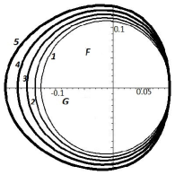
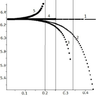
Figure 1. Phase portrait on the plane $(F,G)$ for $G_{+}=0.1$ (left) and the dependence of the period on $G_{+}$ (right) for ${\bf d}=1,2,3,4,5$.

3. The behavior of derivatives

We denote ${\mathcal{D}}=\mbox{div}\,{\bf V}$, $\lambda=\mbox{div}\,{\bf E}$, $J_{ij}=\partial_{x_{i}}{V_{i}}\,\partial_{x_{j}}{V_{j}}-\partial_{x_{j}}{V_{i}}\,\partial_{x_{i}}{V_{j}}$, $i\neq j$, $J=\sum\limits_{i,j=1,\,i\neq j}^{\bf d}J_{ij}.$ The number of terms in the sum is $C^{\bf d}_{2}=\frac{({\bf d}-1){\bf d}}{2}$.

It can be readily shown that

(18) $${\mathcal{D}}={\bf d}\,F+F_{r}\,r,\quad\lambda={\bf d}\,G+G_{r}\,r,\quad J=({\bf d}-1)\,F\,F_{r}\,r+\frac{({\bf d}-1){\bf d}}{2}\,F^{2},$$

therefore

(19) $$2J = 2\,({\bf d}-1)\,{\mathcal{D}}\,F-({\bf d}-1)\,{\bf d}\,F^{2}.$$

Lemma 5.

The solution of the Cauchy problem (8), (9) with a bounded density belongs to the class $C^{1}([0,t_{*})\times\bar{\mathbb{R}}_{+})$ if and only if $\mathcal{D}$ and $\lambda$ are bounded on $[0,t_{*})\times\bar{\mathbb{R}}_{+}$, $t_{*}\leq\infty$.

Proof.

If the density is bounded, then, as follows from Lemma 2, $F$ and $G$ are bounded. If the solution belongs to the class $C^{1}([0,t_{*})\times\bar{\mathbb{R}}_{+})$, then $F_{r}$ and $G_{r}$ are bounded for $t\in[0,t_{*})$. In turn, (18) implies that $\mathcal{D}$ and $\lambda$ are bounded.

On the other hand, if $\mathcal{D}$ and $\lambda$ are bounded together with the density, then $F$ and $G$ are bounded by Lemma 2 and $F_{r}$ and $G_{r}$ are bounded from (18). Since (8) is symmetric hyperbolic system, this implies that the solution is $C^{1}$- smooth globally in $t$ (see [10]). If $\mathcal{D}$ or $\lambda$ tends to $\infty$ as $t\to t_{*}<\infty$, then a singularity forms at the point $t_{*}<\infty$. $\Box$

System (6) implies

$$\displaystyle{\partial{\mathcal{D}}\over\partial t} + ({\bf V}\cdot\nabla{\mathcal{D}})=-{\mathcal{D}}^{2}+2J-\lambda,\qquad\displaystyle{\partial\lambda\over\partial t}+({\bf V}\cdot\nabla\lambda)={\mathcal{D}}(1-\lambda).$$

Taking into account (19), along the characteristic curve, starting from the point $r_{0}$, we obtain

(20) $$\dot{\mathcal{D}}=-{\mathcal{D}}^{2}+2\,({\bf d}-1)\,F\,{\mathcal{D}}-\lambda-({\bf d}-1)\,{\bf d}\,F^{2},\qquad\dot{\lambda}={\mathcal{D}}\,(1-\lambda),$$

a quadratically nonlinear system with the coefficient $F$ found from (11). In fact, (11), (20), can be considered as a system of 4 ODEs for $G,F,{\mathcal{D}},\lambda$, where (11) is separated.

Let us introduce new variables: $u={\mathcal{D}}-{\bf d}\,F$, $v=\lambda-{\bf d}\,G$. Evidently, if $u,v,F,G$ are bounded, then ${\mathcal{D}}$ and $\lambda$ are bounded. Thus, we get a system

(21) $$\dot{u}=-u^{2}-2\,F\,u-v,\quad\dot{v}=-u\,v+(1-{\bf d}\,G)\,u-{\bf d}\,F\,v.$$

Lemma 6.

Assume ${\bf d}\geq 2$. If the data (7) are such that the solution to the Cauchy problem (21),

$$u_{0}(r_{0})=({\mathcal{D}}-{\bf d}F)|_{t=0,\,r=r_{0}},\quad v_{0}(r_{0})=({\lambda}-{\bf d}G)|_{t=0,\,r=r_{0}},$$

is bounded for all fixed $r_{0}\in[0,+\infty)$, $t\in[0,t_{*})$, $t_{*}\leq\infty$, then ${\mathcal{D}}$ and $\lambda$ are bounded and for $t\in[0,t_{*})$ there exists a $C^{1}$-smooth solution to (6), (7) with a positive density.

Proof.

The lemma is a corollary of Lemmas 1, 2 and 5. Indeed, if the solution (21) is bounded, then ${\mathcal{D}}$ and $\lambda$ are bounded, since Lemmas 1 and 2 imply boundedness of $G$ and $F$ and positivity of density. According to the lemma 5, there exists a $C^{1}$-smooth solution to the problem (6), (7) with positive density. $\Box$

Corollary 1.

In the case ${\bf d}\geq 2$ the affine solution to (6), (7) is a globally smooth solution with positive density.

Proof.

System (21) has the trivial solution, it is evidently globally smooth. It corresponds to the affine solution, since $u=F_{r}r=0$ and $v=G_{r}r=0$ imply $F=f(t)$ and $G=g(t)$. The affine solution has the form ${\bf V}=\mathfrak{V}(t){\bf r}$, ${\bf E}=\mathfrak{E}(t){\bf r}$, with $\mathfrak{V}(t)=f(t)\mathfrak{I}$, $\mathfrak{E}(t)=g(t)\mathfrak{I}$, $\mathfrak{I}$ is the identity matrix. $\Box$.

Remark 2.

The fact that the affine solution with positive density is globally smooth for ${\bf d}\geq 2$, follows directly from (12), (13). Indeed, if $F(t,r)=f(t)$, $G(t,r)=g(t)$, then $F$ and $G$ are derivatives of the solution $({\bf V}=F\,{\bf r},{\bf E}=G\,{\bf r})$ with respect to $|{\bf r}|$, and we proved in Sec.2 that they are bounded, if $g(0)<\frac{1}{{\bf d}}$, i.e. density is positive.

4. Linearization and the Radon lemma

Next, we need the following version of the Radon lemma (1927) [7], Theorem 3.1, see also [16].

Theorem 2 (The Radon lemma).

A matrix Riccati equation

(22) $$\dot{W}=M_{21}(t)+M_{22}(t)W-WM_{11}(t)-WM_{12}(t)W,$$

($W=W(t)$ is a matrix $(n\times m)$, $M_{21}$ is a matrix $(n\times m)$, $M_{22}$ is a matrix $(m\times m)$, $M_{11}$ is a matrix $(n\times n)$, $M_{12}$ is a matrix $(m\times n)$) is equivalent to the homogeneous linear matrix equation

(23) $$\dot{Y}=M(t)Y,\quad M=\left(\begin{array}[]{cc}M_{11}&M_{12}\\ M_{21}&M_{22}\end{array}\right),$$

($Y=Y(t)$ is a matrix $(n\times(n+m))$, $M$ is a matrix $((n+m)\times(n+m))$ ) in the following sense.

Let on some interval ${\mathcal{J}}\in\mathbb{R}$ the matrix-function $\,Y(t)=\left(\begin{array}[]{c}\mathfrak{Q}(t)\\ \mathfrak{P}(t)\end{array}\right)$ ($\mathfrak{Q}$ is a matrix $(n\times n)$, $\mathfrak{P}$ is a matrix $(n\times m)$) be a solution of (23) with the initial data

$$Y(0)=\left(\begin{array}[]{c}I\\ W_{0}\end{array}\right)$$

($I$ is the identity matrix $(n\times n)$, $W_{0}$ is a constant matrix $(n\times m)$) and $\det\mathfrak{Q}\neq 0$ on ${\mathcal{J}}$. Then $W(t)=\mathfrak{P}(t)\mathfrak{Q}^{-1}(t)$ is the solution of (22) with $W(0)=W_{0}$ on ${\mathcal{J}}$.

System (21) can be written as (22) with

$$W=\begin{pmatrix}u\\ v\end{pmatrix},\quad M_{11}=\begin{pmatrix}0\\ \end{pmatrix},\quad M_{12}=\begin{pmatrix}1&0\\ \end{pmatrix},$$

$$M_{21}=\begin{pmatrix}0\\ 0\end{pmatrix},\quad M_{22}=\begin{pmatrix}-2\,F&-1\\ 1-d\,G&-d\,F\\ \end{pmatrix}.$$

Thus, we obtain the linear Cauchy problem

(24) $$\begin{pmatrix}\dot{q}\\ \dot{p}_{1}\\ \dot{p}_{2}\\ \end{pmatrix}=\begin{pmatrix}0&1&0\\ 0&-2\,F&-1\\ 0&1-d\,G&-d\,F\\ \end{pmatrix}\begin{pmatrix}q\\ p_{1}\\ p_{2}\\ \end{pmatrix},\quad\begin{pmatrix}q\\ p_{1}\\ p_{2}\\ \end{pmatrix}(0)=\begin{pmatrix}1\\ u_{0}\\ v_{0}\\ \end{pmatrix},$$

with periodical coefficients, known from (11). System (24) implies

$$\ddot{p}_{1}+(2+{\bf d})F\dot{p}_{1}+(1+2({\bf d}-1)F^{2}-(2+{\bf d})G)p_{1}=0.$$

The standard change of the variable $p_{1}(t)=P(t)\,e^{-\frac{{\bf d}+2}{2}\int\limits^{t}_{0}F(\tau)\,d\tau}$ reduces the latter equation to

(25) $$\ddot{P}+{Q}P=0,\quad{Q}=1-\frac{{\bf d}+2}{2}G-\frac{1}{4}({\bf d}-2)({\bf d}-4)F^{2}.$$

Theorem 2 implies that the solution of (21) blows up if and only if $q(t)$ vanishes at some point $t_{*},\,0<t_{*}<\infty$.

From (24) we find

(26) $$q(t)=1+\int\limits_{0}^{t}p_{1}(\tau)\,d\tau=1+\int\limits_{0}^{t}P(\xi)\,e^{-\frac{d+2}{2}\int\limits^{\xi}_{0}F(\tau)\,d\tau}\,d\xi.$$

5. Proof of the main theorem

1. The idea of the proof of the theorem is as follows. It is shown that in the case of initial data of a general form, not related to a simple wave, the function $q$ contains a term that is the product of a periodic function and a growing exponent, and therefore necessarily vanishes in a finite time. Since $q$ serves as the denominator in the expression for $u$ and $v$, the derivative of the solution $({\bf V},{\bf E})$ becomes unbounded in finite time. Since $q$ is expressed in terms of $P$ and $F$ (see (26)), and $F$ is periodic with zero-mean periodicity (see Lemma 3), the property of $q$ to oscillate with increasing amplitude is inherited on the properties of solutions to equation (25), which is an ordinary differential equation with periodic coefficients.

Such equations are described by the Floquet theory (e.g.[4]). It implies that for a periodic ${Q}(t)$ with period $T$, any solution of (25) has the form $P={\mathcal{P}}_{1}(t)e^{\sigma_{1}t}+{\mathcal{P}}_{2}(t)e^{\sigma_{2}t}$, $\sigma_{1}\neq\sigma_{2}$, or $P=e^{\sigma t}({\mathcal{P}}_{1}(t)+{\mathcal{P}}_{2}(t)\,t)$, where the functions ${\mathcal{P}}_{1},{\mathcal{P}}_{2}$ are periodic with period $T$. However, in the general case there is no methods of finding characteristic exponents. In our case ${Q}(t)={Q}(-t)$, therefore (25) has solutions $e^{\mu t}\mathcal{P}(t)$, and $e^{-\mu t}\mathcal{P}(-t)$, $\mathcal{P}$ is $T$-periodic, which can be taken as a fundamental system provided that $\mu$ is real.

2. Let us describe the idea of looking for $\mu$ ([12], section 16.2). Suppose $z(t)$ is a solution of (25) with initial conditions $z(0)=1$, $z^{\prime}(0)=0$. Then

$$z(t)=\frac{1}{2\mathcal{P}(0)}\left(e^{\mu t}\mathcal{P}(t)+e^{-\mu t}\mathcal{P}(-t)\right),$$

since $\mathcal{P}(\pm T)=\mathcal{P}(0)$, $\mathcal{P}^{\prime}(\pm T)=\mathcal{P}^{\prime}(0)$, without loss of generality $\mathcal{P}(0)\neq 0$. Thus,

(27) $$\cosh\mu T=z(T).$$

The boundedness and unboundedness of $e^{\mu t}\mathcal{P}(t)$ (with its derivative and antiderivative) is completely defined by its characteristic exponent $\mu$, defined as a solution of (27). Unboundedness takes place for $|\cosh\mu T|>1$.

In particular, if $z(T)>1$, then $\mu\in\mathbb{R}$, and the general solution of (25) has the form $P=C_{+}e^{\mu t}\mathcal{P}(t)+C_{-}e^{-\mu t}\mathcal{P}(-t)$, with arbitrary constants $C_{+}$, $C_{-}$. Thus, for an arbitrary choice of the data $P$ is unbounded and $q$ oscillates with a growing amplitude.

3. However, for a special choice of the data with $C_{+}=0$ the solution $P$ tends to zero as $t\to\infty$, however $q$, computed with these data, can vanish in a finite point $t_{*}$. Therefore, the respective solution of (21) can blow up or not. If the solution does not blow up, then $u$ and $v$ tend to zero as $t\to\infty$. If this property holds for every $r_{0}\in\bar{\mathbb{R}}_{+}$, then $r_{0}F_{r}(t,r_{0})\to 0$, $r_{0}G_{r}(t,r_{0})\to 0$ and the solution of (6), (7) tends to the affine one uniformly on each compact subset of the half-axis $[0,\infty)$ as $t\to\infty$.

4. Let us show that if $C_{+}=0$ for all characteristic curves, then $G(t,r)$ and $F(t,r)$ are functionally dependent, that is $\Delta(t,r)=F_{r}G_{t}-F_{t}G_{r}=0$ for every $r,t\in\bar{\mathbb{R}}_{+}$.

Differentiating (8) with respect to $r$ and $t$ we get

(28) $$\dot{\Delta}=(({\bf d}+3)F+rF_{r})\Delta$$

along the characteristic curve $r=r(t)$, starting from $r(0)=r_{0}$. Therefore it is enough to check that $\Delta(0,r_{0})=0$.

Since $P(0)=p_{1}(0)=u_{0}=C_{-}\,\mathcal{P}(0)$, $\dot{P}(0)=-C_{-}(\dot{\mathcal{P}}(0)+\mu\mathcal{P}(0))$, $p_{2}(0)=v_{0}=C_{-}(\dot{\mathcal{P}}(0)+\mu\mathcal{P}(0)+\frac{{\bf d}-2}{2}F_{0})$, then

$$\frac{v_{0}}{u_{0}}=\frac{G_{r}(0,r_{0})}{F_{r}(0,r_{0})}=\dot{\mathcal{P}}(0)+\mu\mathcal{P}(0)+\frac{{\bf d}-2}{2}F_{0}.$$

The value of $F_{0}=F(0,r)$, $\mu$, $\mathcal{P}(0)$ also depends on $r_{0}$, we do not write this argument for brevity. We can take the values of $G_{t}(0,r)$ and $F_{t}(0,r)$ from (8). After computations we get

$$\Delta(0,r_{0})=\left((1-{\bf d}G_{0})\,F_{0}+(F_{0}^{2}+G_{0})\left(\frac{{\bf d}-2}{2}\,F_{0}+\mu+\frac{\dot{\mathcal{P}}(0)}{\mathcal{P}(0)}\right)\right)F_{r}(0,r_{0}).$$

For every $r_{0}$ we can choose $G_{0}(r_{0})=G(0,r_{0})$ and $F_{0}(r_{0})=F(0,r_{0})$ such that $\Delta(0,r_{0})=0$, and these data correspond to a functionally dependent $G$ and $F$. In other words, the solution corresponds to a simple wave and, in general, $F=F(G)$. This case we consider in Sec.6.

5. Thus, if we succeed to prove that in our case the characteristic exponent is real, e.g. $z(T)>1$, then we prove the theorem.

First we prove a particular case of Theorem 1.

Proposition 1.

The statement of Theorem 1 holds for the case of small deviation from the zero stationary state.

Proof.

Our reasoning are similar to the asymptotical analysis of the Mathieu equation [12]

$$\ddot{p}(\tau)+(h-2\theta\,\cos 2\tau){p}(\tau)=0,\quad h>0.$$

Solution $z(\tau)$ of the Mathieu equation with initial conditions $z(0)=1$, $\dot{z}(0)=0$ is called the Mathieu C function and can be studied asymptotically. Namely, if $|\theta|\ll 1$, then we can consider $\theta$ as a parameter of regular perturbation, and the solution is found as a series $z=\sum\limits_{k=0}^{\infty}z_{k}(\tau)\theta^{k}$. For every $k$ we get a linear nonhomogeneous equation $\ddot{z_{k}}(\tau)+h{z_{k}}(\tau)=g_{k}(\tau),$ subject to initial data $z_{0}(0)=1$, $\dot{z}_{0}(0)=0$, $z_{k}(0)=\dot{z}_{k}(0)=0$, $k\in\mathbb{N}$, which can be solved in a standard way. Evidently, $z_{0}(\pi)=\cos(\pi\sqrt{h})$. It is easy to check that $z_{1}(\pi)=0$. Thus, we get

$$\cosh\mu\pi=z(\pi)=\cos(\pi\sqrt{h})+\sum\limits_{k=2}^{\infty}z_{k}(\pi)\theta^{k}.$$

It is an analog of formula [12], Sec.16.3 (2).

If $z_{0}(\pi)=1$, then to find the effect of a small perturbation on the characteristic exponent, we calculate $z_{k}(\pi)$ up to the step when $\alpha=z_{k}(\pi)\neq 0$ and get

$$\cosh\mu\pi=z(\pi)=1+\alpha\theta^{k}+o(\theta^{k}),\,\theta\to 0,\,k\geq 2.$$

.

Our situation is more complicated, since we have to consider the periodic coefficient $Q$ in (25) as a series in small initial deviations from zero equilibrium are order $\varepsilon$, $\varepsilon\to 0$. Moreover, the period itself is a series in $\varepsilon$. We expand all functions up to the second order. Namely, if we assume

$$G(t) = \varepsilon G_{1}(t)+\varepsilon^{2}G_{2}(t)+o(\varepsilon^{2}),\quad F(t)=\varepsilon F_{1}(t)+\varepsilon^{2}F_{2}(t)+o(\varepsilon^{2}),$$

$$G(0) = \varepsilon,\quad F(0)=0,$$

then system (11) implies

$$G_{1}(t) = \cos t,\quad F_{1}(t)=-\sin t,$$

$$G_{2}(t) = -\frac{1}{2}+\frac{1}{3}(2+{\bf d})\cos t-\frac{1}{3}(2+{\bf d})\cos 2t,$$

$$F_{2}(t) = -\frac{1}{3}(2+{\bf d})\sin t+\frac{1}{3}(2+{\bf d})\sin 2t.$$

Let us assume

$$z(t)=z_{0}+\varepsilon z_{1}(t)+\varepsilon^{2}z_{2}(t)+o(\varepsilon^{2}),\quad z(0)=1,\,z^{\prime}(0)=0,$$

and substitute to (25). Then

$$z_{0}(t) = \cos t,\quad z_{1}(t)=-\frac{1}{12}(2+{\bf d})(2\cos(t)+\cos 2t-3),$$

$$z_{2}(t) = w\,t\sin t+A_{0}+A_{1}\cos t+A_{2}\cos 2t+A_{3}\cos 3t,$$

where $A_{k}=A_{k}({\bf d})$, $k=0,\dots,3$, $w=\frac{1}{12}({\bf d}-1)({\bf d}-4)\neq 0$.

One can check that $z_{0}(2\pi)=1,$ $z_{1}(2\pi)=z_{2}(2\pi)=0$.

Lemma 4 states that the period of $Q$ is $T=2\pi(1+w\varepsilon^{2}+o(\varepsilon^{2}))$ (see (16)), therefore in the order $\varepsilon^{2}$ we should take into account the change of period. Since $z^{\prime}_{2}(2\pi)=2\pi w$, therefore $z^{\prime}_{2}(2\pi)>0$ if $T>2\pi$ and $z^{\prime}_{2}(2\pi)<0$ if $T<2\pi$, as $T$ changes near $2\pi$. Therefore we have $z_{2}(T)>0$, in a neighborhood of $2\pi$. A more accurate result is given by the expansion $z_{2}(T)=4\pi^{2}w^{2}\varepsilon^{2}+o(\varepsilon^{2})$, $\varepsilon\to 0$. Thus, $z(T)>1$ for $\varepsilon\ll 1$.

The proposition is proved. $\Box$

Recall that in order to prove the theorem in the general case, it is necessary to show that $z(T)>1$, where $z(t)$ is the solution of the equation (25) with initial conditions $z(0)=1$, $z^{\prime}(0)=0$. Because of the complicated form of $F$ and $G$, we cannot hope to obtain this result analytically. Even for the much simpler Mathieu equation, the domains of instability for arbitrary $h$ and $\theta$ (domains on the plane $(h,\theta)$, corresponding to real $\mu$) can only be found numerically [14].

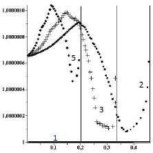
Figure 2. Dependence of $e^{\mu T}$ on $G_{+}$ for ${\bf d}=1$ (and ${\bf d}=4$ till $G_{+}=0.25$), solid line, ${\bf d}=2$, solid circles, ${\bf d}=3$, crosses, ${\bf d}=5$, solid diamonds.

However, we can find the dependence $\mu(G_{+})$, where $G_{+}$ is the greater (positive) root of the equation $F(G)=0$ (see (12), (13)) numerically. Namely, we need to prove that $e^{\mu(G_{+})T(G_{+})}=z(T(G_{+}))>1,$ for all $G_{+}\in(0,\frac{1}{{\bf d}})$.

Let us describe the steps of the computations.

1. Given $G_{+}$ we find the numerical solution of the system (11),

$$\dot{z}=z_{1},\quad\dot{z}_{1}=-Q(G,F)z,$$

with initial data $G(0)=G_{+},\,F(0)=0,\,z(0)=1,\,z_{1}(0)=0$, the Fehlberg fourth-fifth order Runge-Kutta method was used;

2. We find $T$ as a point where $F$ change sign, the step in $t$ is $10^{-7}$;

3. We find $z(T)=e^{\mu T}$ (Fig.2).

Calculations are made with the step $0.005$ in $G_{+}$.

Thus, we see that for ${\bf d}\neq 1$, ${\bf d}\neq 4$, $z(T)>1$ for all possible $G_{+}$, whence follows the conclusion of the theorem.

For ${\bf d}\neq 1$ and ${\bf d}\neq 4$ we have $z(T)=z(2\pi)=1$.

Let us notice that for large ${\bf d}$ possible range of $G_{+}$ is $(0,\frac{1}{{\bf d}}\ll 1)$, therefore any solution can be considered as a small perturbation of the zero state.

Remark 3.

Note that the difference $\Delta=z(T)-1$ can be regarded as a ”measure of instability” in the sense that the greater this difference, the faster the solution blows up. Fig.2 shows that first, if the deviation $\varepsilon=G_{+}$ from the zero stationary state is small enough, $\Delta$ increases monotonically in $\varepsilon$ (from the proof of Proposition 1 one can see that $\Delta=c^{2}\varepsilon^{4}+o(\varepsilon^{4})$, $c=\rm const$). However, then $\Delta$ sharply decreases, remains rather small in a narrow range of $\varepsilon$, and then increases again near the boundary $\frac{1}{{\bf d}}$.

Remark 4.

The result about the breaking of oscillations for physical dimensions ${\bf d}=2$ and ${\bf d}=3$ is confirmed by direct numerics, developed specifically for the cold plasma equations [5], [9].

Remark 5.

Numerical results, performed with high accuracy, suggest that the oscillation does not blow up for ${\bf d}=4$ for all cases of non-negative density $G_{+}<\frac{1}{4}$. We do not currently know of an analytical proof analogous to ${\bf d}=1$ for this conjecture. This problem reduces to finding an additional first integral of the system of four equations (11), (20).

6. Simple waves

Theorem 1 predicts the existence of non-affine solutions with special initial data (7), which are globally smooth and tends to an affine solution as $t\to\infty$.

To construct them, we look for simple waves of the equation (8), such that $F=F(G)$. Thus, (8) reduces to one equation

(29) $$\displaystyle{\partial G\over\partial t}+F(G)r\displaystyle{\partial G\over\partial r}=F(G)(1-{\bf d}G),$$

with $F(G)$ found from (12) or (13), where the constant $C_{\bf d}$ in (12) or (13) does not depend on the initial point $r_{0}$ and the periods of oscillations given as (15) are equal for all characteristics. If we fix $C_{\bf d}$, we obtain the relation between $G$ and $F$ in this special kind of solution, and the corresponding initial data.

Example 1.

Let us construct initial data, corresponding to a simple wave, for ${\bf d}=2$. We choose $G_{0}(r)=\frac{1}{4}e^{-a^{2}r^{2}}$. If we complement this datum by the zero initial velocity $F_{0}(r)=0$, we get a standard laser pulse [5]. Nevertheless, these data are not appropriate for our goal. Instead, we choose $C_{2}=-2$ and find $F_{0}(r)$ from the condition

$$F_{0}^{2}(r)=\frac{1}{2}\,((2G_{0}(r)-1)\ln|1-2G_{0}(r)|+C_{2}(2G_{0}(r)-1)-1),$$

see (12). It can be readily checked that the right-hand side of this expression is positive. Thus,

$$F_{0}(r)=\pm\frac{1}{2}\,\left(1-e^{-a^{2}r^{2}}+\left(\frac{1}{2}\,e^{-a^{2}r^{2}}-1\right)\,\ln\left(1-\frac{1}{2}\,e^{-a^{2}r^{2}}\right)\right)^{\frac{1}{2}}.$$

We can see that $F_{0}(r)\to\pm\frac{1}{2}$ as $r\to\infty$, therefore this initial datum can be considered as a perturbation of the affine initial datum ${\bf V}=\pm\frac{1}{2}\,{\bf r}$.

Further, differentiating (29) with respect to $r$, for $s=G_{r}$ we obtain along the characteristic curve, starting from the point $r_{0}$, the following Bernoulli equation (we take into account (14)):

(30) $$\dot{s}\,=\,-K_{2}(G)\,s^{2}+K_{1}(G)\,s,$$

$$K_{1}(G)=F^{\prime}(G)\,(1-{\bf d}\,G)-(1+{\bf d})F(G),\quad K_{2}=r(G)\,F^{\prime}(G),\quad G=G(t),$$

which has a trivial solution $s=0$, corresponding to the affine solution. If $s(0)\neq 0$, then the derivative of $s(t)$ changes sign on the graph of function $y(t)=\frac{K_{1}(t)}{K_{2}(t)}$, which is periodic and lies from both sides of the axis $s=0$. Thus, $s(t)$ according the scenario of Theorem 1 either oscillates, asymptotically tending to zero or blows up in a finite time.

Due to a complex structure of $G(t)$ it is not possible to obtain a criterium of the blow-up, however, the following result holds.

We call a perturbation of a solution small if the $C^{1}$-norm of the difference between the perturbation and the solution itself is small on every compact subset of the half-axis $[0,\infty)$.

Proposition 2.

A sufficiently small ”simple wave” perturbation of the affine data $({\bf E}_{0}=0,\,{\bf V}_{0}=\beta\,{\bf r})$, $\beta\neq 0$, generates a solution of (6), (7), which does not blow up in a finite time.

Proof.

The small perturbations have the form $G(t)=\epsilon\cos t+o(\epsilon)$, $F=F(G)$, $\epsilon\to 0$. It can be checked that this kind of perturbation is possible only if we choose $C_{2}=-1-2\beta^{2}$ and $C_{\bf d}=\frac{1}{{\bf d}-2}+\beta^{2}$, ${\bf d}\geq 3$, with $\beta^{2}>\epsilon^{2}$. Note that $\beta$ is common to all points $r_{0}\in[0,\infty)$, while $\epsilon$ may depend on $r_{0}$.

Since

$$K_{1}=-({\bf d}+2)\,|\beta|+O(\epsilon),\quad K_{2}=-r_{0}\,|\beta|+O(\epsilon),$$

then neglecting the terms which tends to zero with $\epsilon$ we get from (30)

(31) $$s(t)=\frac{({\bf d}+2)s(0)}{({\bf d}+2)e^{({\bf d}+2)|\beta|t}+(1-e^{({\bf d}+2)|\beta|t})\,r_{0}s(0)},\quad r_{0}\geq 0.$$

Thus, we always can choose sufficiently small $|s(0)|\,r_{0}$ such that the denominator of (31) does not vanish for $t>0$. Thus, $s$ does not blow up and tends exponentially to zero. $\Box$

Remark 6.

The result, similar to Proposition 2 can be proved for the perturbations of an arbitrary affine data $({\bf E}_{0}=\alpha\,{\bf r},\,{\bf V}_{0}=\beta\,{\bf r})$, $\alpha^{2}+\beta^{2}\neq 0$.

It also holds for perturbations in the class of simple waves of the trivial steady state. However, in the latter case, the analysis is more delicate. Note also that the initial perturbation of the trivial state in the class of simple waves cannot be compactly supported or vanish at infinity. Consequently, a solution globally smooth in time tends as $t\to\infty$ to an affine solution, which is itself a small perturbation of the trivial state.

Remark 7.

It is not surprising that there exists a special subclass of solutions to (6) equations that have a more regular behavior than solutions in the general case. For one-dimensional equations of relativistic cold plasma considered in [17] the situation is similar, i.e. simple waves can be globally smooth in time.

7. Behavior of density

Since we reformulated (1) in terms of ${\bf V},{\bf E}$ as (6), (7), we now need to return to the original variables and understand how the singularity in the term of density $n$ arises.

Since $n=1-\lambda$ and $\lambda=\mbox{div}\,{\bf E}$ in notation of Sec.3 (see (5)), then $n\to+\infty$ as $\lambda\to-\infty$. Recall that $\lambda=v+{\bf d}G$, $G$ is bounded (Lemma 2), then $\lambda\to-\infty$ if and only if $v\to-\infty$.

When we consider the solution along a characteristic, starting from a fixed point $r_{0}\geq 0$, then according to Sec.4, $v=\frac{p_{2}}{q}$, where the behavior of $q$ obeys (26), $q(0)=1$, which, in its turn, is defined by $P$. The function $P$ oscillates with exponentially increasing amplitude and in some moment $t_{*}$ the function $q$ becomes zero and $v$ becomes infinity. However, at $0<t<t_{*}$ the denominator $q$ oscillates, being positive, getting closer and closer to zero. So $n(t,r(t))$ also oscillates before going to infinity. The behavior of $\lambda$ that determines $n$ can be studied numerically as a part of the solution of (11), (20).

The easiest way to trace these oscillations is when the blow up occurs at the point $r_{0}=0$, where the maximum of density forms (the physicists call it the ”axial maximum”). The respective characteristic is a straight line (see (10)). In other words, along the characteristic $r_{0}=0$, the solution loses smoothness earlier than along all other characteristics. For this situation the initial data should be especially chosen (as in Example 1). With arbitrary initial data, the behavior of the density is complex, and a supercomputer is required for a thorough analysis. We refer to the results of computations and pictures given in the book [5] for the physical cases ${\bf d}=2$ and ${\bf d}=3$, Ch.4 and 8. The density forms a delta-shape singularity.

References

- [1] A.F. Alexandrov, L.S. Bogdankevich, A.A. Rukhadze, Principles of plasma electrodynamics, Springer series in electronics and photonics, Springer: Berlin Heidelberg, 1984.
- [2] M.Bhatnagar, H.Liu, Critical thresholds in one-dimensional damped Euler-Poisson systems, Mathematical Models and Methods in Applied Sciences, 30(5), 891-916 (2020).
- [3] D.Chae, E. Tadmor, On the finite time blow-up of the Euler-Poisson equations in , Commun. Math. Sci., 6(3), 785-789 (2008).
- [4] C. Chicone, Ordinary Differential Equations with Applications. Springer-Verlag, New York 1999.
- [5] E.V. Chizhonkov, Mathematical aspects of modelling oscillations and wake waves in plasma, CRC Press, 2019.
- [6] R. C. Davidson, Methods in Nonlinear Plasma Theory, Acad. Press, New York, 1972.
- [7] G. Freiling, A survey of nonsymmetric Riccati equations, Linear Algebra and its Applications 351-352, 243-270 (2002).
- [8] V. L. Ginzburg, Propagation of electromagnetic waves in plasma, Pergamon, New York, 1970.
- [9] L.M. Gorbunov, A.A. Frolov, E.V.Chizhonkov, N.E.Andreev, Breaking of nonlinear cylindrical plasma oscillations, Plasma Physics Reports, 36 (4), 345–356 (2010).
- [10] C.M.Dafermos, Hyperbolic conservation laws in continuum physics, The 4th Edition, Berlin-Heidelberg: Springer, 2016.
- [11] S.Engelberg, H.Liu, E.Tadmor, Critical Thresholds in Euler-Poisson Equations, Indiana University Mathematics Journal, 50, 109-157 (2001).
- [12] A. Erdélyi, Higher transcendental functions. Vol. III. Based on notes left by Harry Bateman, Reprint of the 1955 original (Robert E. Krieger Publishing Co., Inc., Melbourne, Fla., 1981).
- [13] E. Esarey, C. B. Schroeder, and W. P. Leemans, Physics of laser-driven plasma-based electron accelerators, Rev. Mod. Phys., 81(2009), 1229-1285.
- [14] N. W.McLachlan, Theory and Applications of Mathieu Functions, Oxford University Press, 1947.
- [15] A. H. Nayfeh, Perturbation methods, John Wiley & Sons, New York, 2000.
- [16] W. T. Reid, Riccati Differential Equations, Academic Press, New York, 1972.
- [17] O.S. Rozanova, E.V. Chizhonkov, On the conditions for the breaking of oscillations in a cold plasma, Z. Angew. Math. Phys., 72 (2021), 13.
- [18] O. Rozanova, E.Chizhonkov, M.Delova, Exact thresholds in the dynamics of cold plasma with electron-ion collisions, AIP Conference Proceedings, 2302 (1), 060012 (2020), https://doi.org/10.1063/5.0033619
- [19] C.Tan, Eulerian dynamics in multidimensions with radial symmetry, SIAM Journal on Mathematical Analysis, 53 (3), 3040-3071 (2021).
- [20] D. Wei, E. Tadmor, H. Bae. Critical Thresholds in multi-dimensional Euler-Poisson equations with radial symmetry. Commun. Math. Sci., 10(1):75-86, 2012.