Abstract

Quantum reservoir computing is a machine-learning approach designed to exploit the dynamics of quantum systems with memory to process information. As an advantage, it presents the possibility to benefit from the quantum resources provided by the reservoir combined with a simple and fast training strategy. In this work, this technique is introduced with a quantum reservoir of spins and it is applied to find the ground-state energy of an additional quantum system. The quantum reservoir computer is trained with a linear model to predict the lowest energy of a particle in the presence of different speckle-disorder potentials. The performance of the task is analyzed with a focus on the observable quantities extracted from the reservoir and it shows to be enhanced when two-qubit correlations are employed.

1 1 0 https://doi.org/ Quantum Reservoir Computing for Speckle-Disorder Potentials Quantum Reservoir Computing for Speckle-Disorder Potentials Pere Mujal ¹ Pere Mujal Mujal, P. Correspondence: peremujal@ifisc.uib-csic.es

1 Introduction

In the last few years, the study of quantum systems has taken advantage of the increasing interest and the developments of machine learning techniques to face both theoretical and experimental challenges, which has lead to the emergence of the broad field of quantum machine learning Biamonte et al. (2017); Dunjko and Briegel (2018); Carrasquilla (2020); Schuld et al. (2015); Carleo et al. (2019). Some successful examples of the use of machine learning include, among others, the detection and classification of quantum phases Kottmann et al. (2020); Dong et al. (2019); Carrasquilla and Melko (2017); Wang (2016); Rem et al. (2019); Huembeli et al. (2018); Canabarro et al. (2019); Schindler et al. (2017), the prediction of the ground-state energy and other characteristic quantities of quantum systems Mills et al. (2017); Pilati and Pieri (2020, 2019); Mujal et al. (2021), and the enhanced control and readout in experimental setups Wigley et al. (2016); Tranter et al. (2018); Barker et al. (2020); Flurin et al. (2020). Additionally, many efforts are devoted to develop machine-learning algorithms that exploit quantum resources, aiming to find a quantum advantage in performing tasks. Quantum reservoir computing (QRC) and related approaches belong to this last category Mujal et al. (2021); Ghosh et al. (2021).

The concept of QRC was introduced in Fujii and Nakajima (2017) as an extension to the quantum realm of classical reservoir computing (RC) Lukoševičius and Jaeger (2009); Jaeger and Haas (2004); Maass and Markram (2004); Brunner et al. (2019). The main idea behind RC, as an unconventional computing method Konkoli (2017); Adamatzky et al. (2007), is the use of the natural dynamics of systems to process information, together with a simplified training strategy Butcher et al. (2013). For supervised learning techniques, for instance in the case of deep neural networks, one of the major drawbacks is the training process of models with typically thousands of free parameters to be optimally adjusted, which requires a lot of computational resources and/or time. Instead of that, in RC, the connections between the constituents of the reservoir are kept fixed and only the output quantities from the reservoir are involved in the training process and could be easily retrained for a different purpose. This scheme has shown to be sufficient to achieve very good performances in diverse tasks Lukoševičius (2012); Antonik et al. (2019); Alfaras et al. (2019); Pathak et al. (2018).

Quantum reservoirs are good candidates to be exploited for computational purposes for several reasons. First of all, the number of degrees of freedom in quantum systems increases exponentially with the number of constituents. Therefore, with relatively small systems, a large state space is available, which has been shown to be beneficial, i.e. it increases the memory capacity Schuld and Killoran (2019); Abbas et al. (2021); Fujii and Nakajima (2017); Nokkala et al. (2021); Martínez-Peña et al. (2020). In second place, the presence of entanglement can also contribute to achieve a quantum advantage when quantum correlations are exploited Martínez-Peña et al. (2020). Finally, there exist several proposals suitable to be implemented in a wide variety of experimental platforms to realize not only classical tasks but also quantum ones Mujal et al. (2021), for instance, entanglement detection Ghosh et al. (2019), quantum state tomography Ghosh et al. (2020) and quantum state preparation Ghosh et al. (2019); Krisnanda et al. (2021).

In this article, the possibility of using a quantum reservoir to study another quantum system is explored as an alternative to classical machine-learning models. A first goal in this work is to show that a quantum reservoir can be used to make predictions on the ground-state energy of a quantum particle in a speckle-disorder potential Aspect and Inguscio (2009) by only providing as an input this external potential and by using only a linear model to train the output observables. This problem is of relevance for understanding the Anderson localization phenomenon in quantum systems due to the presence of disorder, which determines their transport properties Anderson (1958). Additionally, we aim to analyze the effect on the performance when two-body quantum correlations in the reservoir are used compared with one-body observables for the mentioned task.

This work is organized as follows. In Section 2, the details on the quantum system in study are provided together with the database used. The description of how the input is encoded into the quantum reservoir is found in Section 3. In Section 4, the characteristics of the quantum reservoir system are explained. In Section 5, the quantum reservoir computing procedure is presented with the mathematical description of the state of the reservoir and its observables. The expressions of the trained models and an analysis of their performance are given in Section 6. Finally, the discussion of the results and the conclusions are in Section 7.

2 Database of Speckle-Disorder Potentials and Ground-State Energies

The problem to be addressed with the model proposed in this work consists in finding the lowest energy of the following Hamiltonian, which describes a particle of mass $m$ in one dimension with position $x$ in the presence of an external potential $V(x)$:

$$\mathcal{H}=-\frac{\hbar^{2}}{2m}\frac{\partial^{2}}{\partial x^{2}}+V(x),$$ (1)

where $\hbar$ is the reduced Planck constant. $V(x)$ is a speckle potential that in cold-atoms experiments is created by means of optical fields passing through a diffusion plate Clément et al. (2006); Billy et al. (2008); Roati et al. (2008) and can be numerically produced with Gaussian random numbers Modugno (2006); Huntley (1989). This potential introduces disorder into the system and originates the Anderson localization phenomenon Anderson (1958); Aspect and Inguscio (2009).

In previous studies, classical machine-learning models with convolutional neural networks have shown to be able to make very good predictions on the first energies of this system and for different system sizes by applying transfer-learning protocols Pilati and Pieri (2019). Additionally, the extension to the system with few repulsively interacting bosons Mujal et al. (2019) has also been explored including the particle number as an additional feature to the trained model Mujal et al. (2021).

The database used in this article is part of the database used in  Mujal et al. (2021), which is publicly available at  Mujal et al. (2020). In this work, the first 10000 speckle-potential instances of the single-particle dataset and their corresponding ground-state energies are used. The energies in the database were computed numerically by means of exact diagonalization as explained in Mujal et al. (2019) and in more detail in Mujal (2019).

3 Input Ecoding into the Quantum Reservoir

The values of each different speckle-potential instance in the dataset are provided in a discrete grid in space of $K=1024$ points, $V(x_{k})=V_{k}$, with $k=1,\,...\,,K$. Therefore, our input is a set of vectors of size $1024$ where the spatial structure of each potential is given by the order of the elements. For this reason, the values of the potential are introduced into the dynamics of the quantum reservoir in the same order. From the point of view of the quantum reservoir, a given speckle potential corresponds to an external time-dependent signal fed at discrete times, $t=k\Delta t$.

The input at a given time, $V_{k}$, is encoded in one of the qubits of the system (See Figure 1), qubit 1, by setting its state as Martínez-Peña et al. (2021); Fujii and Nakajima (2017); Kutvonen et al. (2020); Martínez-Peña et al. (2020):

$$\ket{\psi_{k}}=\sqrt{1-s_{k}}\ket{0}+\sqrt{s_{k}}\ket{1},$$ (2)

where $s_{k}=V_{k}/V_{\textnormal{max}}$ and the value of $V_{\textnormal{max}}$ is always the same and fixed as the maximum reached among all the $10000$ speckle instances in the dataset. In this way, $s_{k}\in[0,1]$ to have a properly normalized state for the qubit and all inputs are re-scaled the same quantity. The basis states that are used are the eigenstates of the Pauli matrix $\hat{\sigma}^{z}$, namely $\hat{\sigma}^{z}\ket{0}=\ket{0}$ and $\hat{\sigma}^{z}\ket{1}=-\ket{1}$.

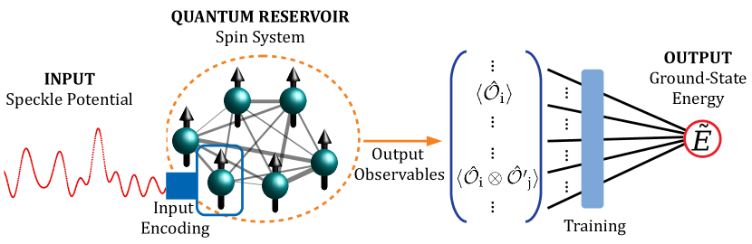
Figure 1: Schematic representation of the use of a quantum reservoir to predict the ground-state energy of a quantum particle in a speckle potential. The spatial-dependent values of the speckle potential are transformed into a time-dependent signal fed into the state of one spin of the reservoir at discrete time steps. The quantum reservoir system evolves between input injections. Different observables are extracted from the reservoir system and used in the training process to produce ground-state energy predictions.

4 Hamiltonian of the Reservoir of Spins

The quantum reservoir employed in this work is a system consisting of $N=6$ spins (or qubits). The unitary dynamics of this system are governed by the following transverse-field Ising Hamiltonian:

$$\hat{H}_{\textnormal{R}}=\frac{1}{2}\sum_{i=1}^{N}h\hat{\sigma}_{i}^{z}+\sum_{i<j}^{N}J_{ij}\hat{\sigma}_{i}^{x}\hat{\sigma}_{j}^{x},$$ (3)

where $\hat{\sigma}_{i}^{z}$ and $\hat{\sigma}_{j}^{x}$ are Pauli matrices acting on qubits $i$ and $j$, respectively. The spin-spin couplings $J_{ij}$, represented as lines of different thickness in Figure 1, are randomly generated once from a uniform distribution in the interval $[-J_{s}/2,J_{s}/2]$ and then kept constant. We work on a system of units with $\hbar=1$ and $J_{s}=1$. The time intervals $\Delta t$, are expressed in units of $1/J_{s}$, and $h$, that corresponds to an external magnetic field in the z direction, is fixed at $h=10J_{s}$, such that the system is in the appropriate dynamical regime Martínez-Peña et al. (2021). This kind of system was in the original proposal of QRC in Fujii and Nakajima (2017) and has been extensively studied for information processing purposes in further several works Chen and Nurdin (2019); Nakajima et al. (2019); Martínez-Peña et al. (2020, 2021); Kutvonen et al. (2020); Mujal et al. (2021); Tran and Nakajima (2020).

5 Quantum Reservoir Computer Operation

The role of the quantum reservoir is to provide a map between the input speckle to the output observables. They carry the information about the input that has been processed during the time-evolution of the reservoir system. The memory of the system, for the present purposes, is exploited within each instance. However, the system is reset before the introduction of each speckle-potential at time $t=0$. In this way, there are no dependencies between consecutive instances. The general scheme of the procedure is depicted in Figure 1.

The density matrix that describes the quantum state of the reservoir of spins before the injection of each potential reads:

$$\rho_{0}=\ket{0,\,...\,,0}\bra{0,\,...\,,0}.$$ (4)

Afterwards, for a given speckle-potential instance, the state of the reservoir at each time step $k$, is given by:

$$\rho_{k}=e^{-i\hat{H}_{\textnormal{R}}\Delta t}\left(\ket{\psi_{k}}\bra{\psi_{k}}\otimes\textnormal{Tr}_{1}({\rho}_{k-1})\right)e^{i\hat{H}_{\textnormal{R}}\Delta t},$$ (5)

where $\textnormal{Tr}_{1}()$ indicates the partial trace with respect to the first qubit. The dependence on the speckle points, $V_{k}$, is through fixing the state of the first qubit, $\ket{\psi_{k}}\bra{\psi_{k}}$, in the form of Equation (2). Between input injections, there is a unitary evolution of the state of the reservoir of $\Delta t$ duration governed by the Hamiltonian in (3).

From the state of the reservoir, the expectation values of the following single-qubit observables at each time step $k$ are computed as:

$$\langle\hat{\sigma}^{\alpha}_{i}\rangle_{k}=\textnormal{Tr}\left(\rho_{k}\hat{\sigma}^{\alpha}_{i}\right),$$ (6)

for all spins, $i=1,\,....\,N$, and in the three directions $\alpha=x,y,z$. Afterwards, the average over all time steps is taken to obtain:

$$\langle\hat{\sigma}^{\alpha}_{i}\rangle\equiv\frac{1}{K}\sum_{k=1}^{K}\langle\hat{\sigma}^{\alpha}_{i}\rangle_{k}.$$ (7)

Similarly, the expectation values of the two-qubit observables are calculated,

$$\langle\hat{\sigma}^{\alpha}_{i}\hat{\sigma}^{\beta}_{j}\rangle_{k}=\textnormal{Tr}\left(\rho_{k}\hat{\sigma}^{\alpha}_{i}\hat{\sigma}^{\beta}_{j}\right),$$ (8)

and

$$\langle\hat{\sigma}^{\alpha}_{i}\hat{\sigma}^{\beta}_{j}\rangle\equiv\frac{1}{K}\sum_{k=1}^{K}\langle\hat{\sigma}^{\alpha}_{i}\hat{\sigma}^{\beta}_{j}\rangle_{k},$$ (9)

with $i<j$ and $\alpha,\beta=x,y,z$.

6 Training and Predictions of the Models

From the output observables of the quantum reservoir, two models to make predictions, $\tilde{E}$, on the ground-state energies are proposed. Both are constructed by fitting a least-squares linear model with the training dataset, which corresponds to the first 7500 speckle instances and target energies $E$. The quality of the models is tested with the remaining 2500 potentials and it is quantified by the mean absolut error (MAE),

$$\textnormal{MAE}=\frac{1}{M}\sum_{l=1}^{M}|E_{l}-\tilde{E}_{l}|,$$ (10)

and the coefficient of determination

$$R^{2}=1-\frac{\sum_{l=1}^{M}(E_{l}-\tilde{E}_{l})^{2}}{\sum_{l=1}^{M}(\bar{E}-E_{l})^{2}},$$ (11)

where $\bar{E}$ is the mean energy $\bar{E}\equiv(1/M)\sum_{l=1}^{M}E_{l}$, and $M$ is the number of instances, $M=7500$ for the training data, and $M=2500$ for the test data. If $R^{2}=0$, the predicted and the target energies are not linearly related, whereas for $R^{2}=1$ the predictions are perfect.

In the first case, the single-qubit observables in Equation (7) are employed and the final output, $\tilde{E}$, for each instance is written as:

$$\begin{gathered}\tilde{E}=v_{0}+\sum_{i=1}^{N}\left(v_{1,i}\langle\hat{\sigma}^{x}_{i}\rangle+v_{2,i}\langle\hat{\sigma}^{y}_{i}\rangle+v_{3,i}\langle\hat{\sigma}^{z}_{i}\rangle+v_{4,i}\langle\hat{\sigma}^{x}_{i}\rangle^{2}+v_{5,i}\langle\hat{\sigma}^{y}_{i}\rangle^{2}+v_{6,i}\langle\hat{\sigma}^{z}_{i}\rangle^{2}\right.\\ \left.+v_{7,i}\langle\hat{\sigma}^{x}_{i}\rangle\langle\hat{\sigma}^{y}_{i}\rangle+v_{8,i}\langle\hat{\sigma}^{y}_{i}\rangle\langle\hat{\sigma}^{z}_{i}\rangle+v_{9,i}\langle\hat{\sigma}^{z}_{i}\rangle\langle\hat{\sigma}^{x}_{i}\rangle+v_{10,i}\langle\hat{\sigma}^{x}_{i}\rangle\langle\hat{\sigma}^{y}_{i}\rangle\langle\hat{\sigma}^{z}_{i}\rangle\right).\end{gathered}$$ (12)

In this last model and for a system with $N=6$, there are 61 free parameters, $v$ with the corresponding labels, that are optimized during the training.

In the second case, there are 451 different weights $w$ to be adjusted when the two-qubit quantities in Equation (9) are used in the similar following way:

$$\begin{gathered}\tilde{E}=w_{0}+\sum_{i<j=1}^{N}\left(w_{1,i,j}\langle\hat{\sigma}^{x}_{i}\hat{\sigma}^{x}_{j}\rangle+w_{2,i,j}\langle\hat{\sigma}^{y}_{i}\hat{\sigma}^{y}_{j}\rangle+w_{3,i,j}\langle\hat{\sigma}^{z}_{i}\hat{\sigma}^{z}_{j}\rangle\right.\\ \left.+w_{4,i,j}\langle\hat{\sigma}^{x}_{i}\hat{\sigma}^{x}_{j}\rangle^{2}+w_{5,i,j}\langle\hat{\sigma}^{y}_{i}\hat{\sigma}^{y}_{j}\rangle^{2}+w_{6,i,j}\langle\hat{\sigma}^{z}_{i}\hat{\sigma}^{z}_{j}\rangle^{2}+w_{7,i,j}\langle\hat{\sigma}^{x}_{i}\hat{\sigma}^{x}_{j}\rangle\langle\hat{\sigma}^{y}_{i}\hat{\sigma}^{y}_{j}\rangle\right.\\ \left.+w_{8,i,j}\langle\hat{\sigma}^{y}_{i}\hat{\sigma}^{y}_{j}\rangle\langle\hat{\sigma}^{z}_{i}\hat{\sigma}^{z}_{j}\rangle+w_{9,i,j}\langle\hat{\sigma}^{z}_{i}\hat{\sigma}^{z}_{j}\rangle\langle\hat{\sigma}^{x}_{i}\hat{\sigma}^{x}_{j}\rangle+w_{10,i,j}\langle\hat{\sigma}^{x}_{i}\hat{\sigma}^{x}_{j}\rangle\langle\hat{\sigma}^{y}_{i}\hat{\sigma}^{y}_{j}\rangle\langle\hat{\sigma}^{z}_{i}\hat{\sigma}^{z}_{j}\rangle\right)\\ +\sum_{i\neq j=1}^{N}\left(w_{11,i,j}\langle\hat{\sigma}^{x}_{i}\hat{\sigma}^{y}_{j}\rangle+w_{12,i,j}\langle\hat{\sigma}^{y}_{i}\hat{\sigma}^{z}_{j}\rangle+w_{13,i,j}\langle\hat{\sigma}^{z}_{i}\hat{\sigma}^{x}_{j}\rangle\right.\\ \left.+w_{14,i,j}\langle\hat{\sigma}^{x}_{i}\hat{\sigma}^{y}_{j}\rangle^{2}+w_{15,i,j}\langle\hat{\sigma}^{y}_{i}\hat{\sigma}^{z}_{j}\rangle^{2}+w_{16,i,j}\langle\hat{\sigma}^{z}_{i}\hat{\sigma}^{x}_{j}\rangle^{2}+w_{17,i,j}\langle\hat{\sigma}^{x}_{i}\hat{\sigma}^{y}_{j}\rangle\langle\hat{\sigma}^{y}_{i}\hat{\sigma}^{z}_{j}\rangle\right.\\ \left.+w_{18,i,j}\langle\hat{\sigma}^{y}_{i}\hat{\sigma}^{z}_{j}\rangle\langle\hat{\sigma}^{z}_{i}\hat{\sigma}^{x}_{j}\rangle+w_{19,i,j}\langle\hat{\sigma}^{z}_{i}\hat{\sigma}^{x}_{j}\rangle\langle\hat{\sigma}^{x}_{i}\hat{\sigma}^{y}_{j}\rangle+w_{20,i,j}\langle\hat{\sigma}^{x}_{i}\hat{\sigma}^{y}_{j}\rangle\langle\hat{\sigma}^{y}_{i}\hat{\sigma}^{z}_{j}\rangle\langle\hat{\sigma}^{z}_{i}\hat{\sigma}^{x}_{j}\rangle\right).\end{gathered}$$ (13)

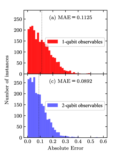
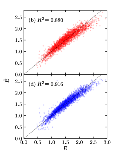
Figure 2: (Left) Absolut error distributions corresponding to the test data of the model with single-qubit observables in (a) and two-qubit observables in (c). A dashed line indicates the mean absolut error (MAE). (Right) Predicted energies $\tilde{E}$ as a function of the target energies $E$ for the test data. In (b) the predictions are made with the model in Equation (12) and in (d) with the one in  (13). The ideal situation, with perfect predictions, is depicted with a dashed line and would correspond to $R^{2}=1$.

As in the neural-network models in Pilati and Pieri (2019) and Mujal et al. (2021), the predictions $\tilde{E}$ are functions of the speckle points in space. In the present case, the required nonlinear dependence of the outputs on the input values of the potential are, in general, guaranteed by both the form of input encoding in Equation (2) and an appropriate choice of the Hamiltonian parameters Mujal et al. (2021). Beyond that, further nonlinear dependencies on the input have been introduced by combining the observables in (12) and (13) because it is beneficial to increase the performance without losing the linearity of the models.

The quality of the predictions of the two models is shown in Figure 2. Remarkably, the model that produces the predictions from the single-qubit observables of the reservoir with only 61 optimized parameters is able to learn from the training data without overfitting. The MAE and $R^{2}$ for the training data are 0.1126 and 0.8808, respectively, and practically equal to the values of the test data provided in Figure 2. In panel (a), in the distribution of the absolute error, there is a considerable number of speckle instances whose error is below the MAE. Moreover in panel (b), there is a clear correlation between the target energies and the predicted ones for the test data reflected on the large value of $R^{2}=0.880$, which is close to 0.9. If the model of two-qubit observables is employed instead, the accuracy of the predictions is, in general, improved. The peak of the distribution in panel (c) of the absolute error is sharper and closer to 0, as well as the value of the MAE. In accordance, in the scatter plot in panel (d) the value of $R^{2}$ surpasses 0.9 and we are closer to the ideal situation. Also in this case with much more free parameters, 451, the comparison between the values of the MAE$=0.0833$ and $R^{2}=0.936$ for the training data and the test data in panels (c) and (d) indicates that there is not a significant overfitting problem.

7 Discussion and Conclusions

The results obtained with the models proposed in this work show that a quantum reservoir is suitable to be used to address the problem of making predictions on the ground-state energy of different speckle-disorder potentials. By following this approach, the computational capabilities of the quantum dynamics of the system are exploited and linear models with the observables of the quantum reservoir are sufficient to achieve a noticeable accuracy. In this way, we have taken advantage of both a simple and fast training strategy and the presence of quantum correlations. This paves the way to further develop models that follow a similar strategy, for instance, for systems of interacting particles in the presence of a speckle potential.

In fact, for practical purposes, the quality of the predictions should be increased in order to compete with state-of-the-art deep convolutional neural networks. To reach this aim, several strategies could be followed. It would be interesting to explore the effect of changing the form of the input encoding into the quantum reservoir and to study its impact on the quality of the predictions of the models. In addition to that, in the present work we have only explored the possibility of using single-qubit and two-qubit observables. The extension to three-body quantities and beyond should be considered and could contribute to improve the performance. This would lead to more flexible models, as the number of observables would be increased as well as the number of free parameters. Additionally, in a similar way, increasing the number of spins would enlarge the Hilbert space and increase the capabilities of the quantum reservoir. Regarding the Hamiltonian of the reservoir system, the values of the couplings and the external magnetic field could be seen as hyperparameters. As the performance in realizing the task depends on their values, to improve the results presented in this work, they could be optimized by defining an additional validation dataset.

This research was funded by: the Spanish State Research Agency, through the Severo Ochoa and María de Maeztu Program for Centers and Units of Excellence in R&D, grant number MDM-2017-0711; Comunitat Autònoma de les Illes Balears, Govern de les Illes Balears, through the QUAREC project, grant number PRD2018/47; the Spanish State Research Agency through the QUARESC project, grant numbers PID2019-109094GB-C21 and -C22/AEI/10.13039/501100011033.

The data used in this study are openly available in Zenodo at Mujal et al. (2020).

References

- Biamonte et al. (2017) Biamonte, J.; Wittek, P.; Pancotti, N.; Rebentrost, P.; Wiebe, N.; Lloyd, S. Quantum machine learning. Nature 2017, 549, 195–202. doi:\changeurlcolorblack10.1038/nature23474.
- Dunjko and Briegel (2018) Dunjko, V.; Briegel, H.J. Machine learning & artificial intelligence in the quantum domain: a review of recent progress. Reports on Progress in Physics 2018, 81, 074001. doi:\changeurlcolorblack10.1088/1361-6633/aab406.
- Carrasquilla (2020) Carrasquilla, J. Machine learning for quantum matter. Advances in Physics: X 2020, 5, 1797528. doi:\changeurlcolorblack10.1080/23746149.2020.1797528.
- Schuld et al. (2015) Schuld, M.; Sinayskiy, I.; Petruccione, F. An introduction to quantum machine learning. Contemporary Physics 2015, 56, 172–185. doi:\changeurlcolorblack10.1080/00107514.2014.964942.
- Carleo et al. (2019) Carleo, G.; Cirac, I.; Cranmer, K.; Daudet, L.; Schuld, M.; Tishby, N.; Vogt-Maranto, L.; Zdeborová, L. Machine learning and the physical sciences. Rev. Mod. Phys. 2019, 91, 045002. doi:\changeurlcolorblack10.1103/RevModPhys.91.045002.
- Kottmann et al. (2020) Kottmann, K.; Huembeli, P.; Lewenstein, M.; Acín, A. Unsupervised Phase Discovery with Deep Anomaly Detection. Phys. Rev. Lett. 2020, 125, 170603. doi:\changeurlcolorblack10.1103/PhysRevLett.125.170603.
- Dong et al. (2019) Dong, X.Y.; Pollmann, F.; Zhang, X.F. Machine learning of quantum phase transitions. Phys. Rev. B 2019, 99, 121104. doi:\changeurlcolorblack10.1103/PhysRevB.99.121104.
- Carrasquilla and Melko (2017) Carrasquilla, J.; Melko, R.G. Machine learning phases of matter. Nature Physics 2017, 13, 431–434. doi:\changeurlcolorblack10.1038/nphys4035.
- Wang (2016) Wang, L. Discovering phase transitions with unsupervised learning. Phys. Rev. B 2016, 94, 195105. doi:\changeurlcolorblack10.1103/PhysRevB.94.195105.
- Rem et al. (2019) Rem, B.S.; Käming, N.; Tarnowski, M.; Asteria, L.; Fläschner, N.; Becker, C.; Sengstock, K.; Weitenberg, C. Identifying quantum phase transitions using artificial neural networks on experimental data. Nature Physics 2019, 15, 917–920. doi:\changeurlcolorblack10.1038/s41567-019-0554-0.
- Huembeli et al. (2018) Huembeli, P.; Dauphin, A.; Wittek, P. Identifying quantum phase transitions with adversarial neural networks. Phys. Rev. B 2018, 97, 134109. doi:\changeurlcolorblack10.1103/PhysRevB.97.134109.
- Canabarro et al. (2019) Canabarro, A.; Fanchini, F.F.; Malvezzi, A.L.; Pereira, R.; Chaves, R. Unveiling phase transitions with machine learning. Phys. Rev. B 2019, 100, 045129. doi:\changeurlcolorblack10.1103/PhysRevB.100.045129.
- Schindler et al. (2017) Schindler, F.; Regnault, N.; Neupert, T. Probing many-body localization with neural networks. Phys. Rev. B 2017, 95, 245134. doi:\changeurlcolorblack10.1103/PhysRevB.95.245134.
- Mills et al. (2017) Mills, K.; Spanner, M.; Tamblyn, I. Deep learning and the Schrödinger equation. Phys. Rev. A 2017, 96, 042113. doi:\changeurlcolorblack10.1103/PhysRevA.96.042113.
- Pilati and Pieri (2020) Pilati, S.; Pieri, P. Simulating disordered quantum Ising chains via dense and sparse restricted Boltzmann machines. Phys. Rev. E 2020, 101, 063308. doi:\changeurlcolorblack10.1103/PhysRevE.101.063308.
- Pilati and Pieri (2019) Pilati, S.; Pieri, P. Supervised machine learning of ultracold atoms with speckle disorder. Scientific Reports 2019, 9, 5613. doi:\changeurlcolorblack10.1038/s41598-019-42125-w.
- Mujal et al. (2021) Mujal, P.; Àlex Martínez Miguel.; Polls, A.; Juliá-Díaz, B.; Pilati, S. Supervised learning of few dirty bosons with variable particle number. SciPost Phys. 2021, 10, 73. doi:\changeurlcolorblack10.21468/SciPostPhys.10.3.073.
- Wigley et al. (2016) Wigley, P.B.; Everitt, P.J.; van den Hengel, A.; Bastian, J.W.; Sooriyabandara, M.A.; McDonald, G.D.; Hardman, K.S.; Quinlivan, C.D.; Manju, P.; Kuhn, C.C.N.; Petersen, I.R.; Luiten, A.N.; Hope, J.J.; Robins, N.P.; Hush, M.R. Fast machine-learning online optimization of ultra-cold-atom experiments. Scientific Reports 2016, 6, 25890. doi:\changeurlcolorblack10.1038/srep25890.
- Tranter et al. (2018) Tranter, A.D.; Slatyer, H.J.; Hush, M.R.; Leung, A.C.; Everett, J.L.; Paul, K.V.; Vernaz-Gris, P.; Lam, P.K.; Buchler, B.C.; Campbell, G.T. Multiparameter optimisation of a magneto-optical trap using deep learning. Nature Communications 2018, 9, 4360. doi:\changeurlcolorblack10.1038/s41467-018-06847-1.
- Barker et al. (2020) Barker, A.J.; Style, H.; Luksch, K.; Sunami, S.; Garrick, D.; Hill, F.; Foot, C.J.; Bentine, E. Applying machine learning optimization methods to the production of a quantum gas. Machine Learning: Science and Technology 2020, 1, 015007. doi:\changeurlcolorblack10.1088/2632-2153/ab6432.
- Flurin et al. (2020) Flurin, E.; Martin, L.S.; Hacohen-Gourgy, S.; Siddiqi, I. Using a Recurrent Neural Network to Reconstruct Quantum Dynamics of a Superconducting Qubit from Physical Observations. Phys. Rev. X 2020, 10, 011006. doi:\changeurlcolorblack10.1103/PhysRevX.10.011006.
- Mujal et al. (2021) Mujal, P.; Martínez-Peña, R.; Nokkala, J.; García-Beni, J.; Giorgi, G.L.; Soriano, M.C.; Zambrini, R. Opportunities in Quantum Reservoir Computing and Extreme Learning Machines. Advanced Quantum Technologies 2021, p. 2100027. doi:\changeurlcolorblackhttps://doi.org/10.1002/qute.202100027.
- Ghosh et al. (2021) Ghosh, S.; Nakajima, K.; Krisnanda, T.; Fujii, K.; Liew, T.C.H. Quantum Neuromorphic Computing with Reservoir Computing Networks. Advanced Quantum Technologies 2021, 4, 2100053. doi:\changeurlcolorblackhttps://doi.org/10.1002/qute.202100053.
- Fujii and Nakajima (2017) Fujii, K.; Nakajima, K. Harnessing Disordered-Ensemble Quantum Dynamics for Machine Learning. Phys. Rev. Applied 2017, 8, 024030. doi:\changeurlcolorblack10.1103/PhysRevApplied.8.024030.
- Lukoševičius and Jaeger (2009) Lukoševičius, M.; Jaeger, H. Reservoir computing approaches to recurrent neural network training. Comput. Sci. Rev. 2009, 3, 127–149. doi:\changeurlcolorblackhttps://doi.org/10.1016/j.cosrev.2009.03.005.
- Jaeger and Haas (2004) Jaeger, H.; Haas, H. Harnessing Nonlinearity: Predicting Chaotic Systems and Saving Energy in Wireless Communication. Science 2004, 304, 78–80. doi:\changeurlcolorblack10.1126/science.1091277.
- Maass and Markram (2004) Maass, W.; Markram, H. On the computational power of circuits of spiking neurons. Journal of Computer and System Sciences 2004, 69, 593–616. doi:\changeurlcolorblackhttps://doi.org/10.1016/j.jcss.2004.04.001.
- Brunner et al. (2019) Brunner, D.; Soriano, M.C.; Van der Sande, G. Photonic Reservoir Computing: Optical Recurrent Neural Networks; Walter de Gruyter GmbH & Co KG, 2019.
- Konkoli (2017) Konkoli, Z. On reservoir computing: from mathematical foundations to unconventional applications. In Advances in unconventional computing; Springer, 2017; pp. 573–607.
- Adamatzky et al. (2007) Adamatzky, A.; Bull, L.; De Lacy Costello, B.; Stepney, S.; Teuscher, C. Unconventional Computing 2007; Luniver Press, 2007.
- Butcher et al. (2013) Butcher, J.B.; Verstraeten, D.; Schrauwen, B.; Day, C.R.; Haycock, P.W. Reservoir computing and extreme learning machines for non-linear time-series data analysis. Neural Networks 2013, 38, 76–89. doi:\changeurlcolorblackhttps://doi.org/10.1016/j.neunet.2012.11.011.
- Lukoševičius (2012) Lukoševičius, M. A practical guide to applying echo state networks. In Neural networks: Tricks of the trade; Springer, 2012; pp. 659–686.
- Antonik et al. (2019) Antonik, P.; Marsal, N.; Brunner, D.; Rontani, D. Human action recognition with a large-scale brain-inspired photonic computer. Nature Machine Intelligence 2019, 1, 530–537. doi:\changeurlcolorblack10.1038/s42256-019-0110-8.
- Alfaras et al. (2019) Alfaras, M.; Soriano, M.C.; Ortín, S. A Fast Machine Learning Model for ECG-Based Heartbeat Classification and Arrhythmia Detection. Frontiers in Physics 2019, 7, 103. doi:\changeurlcolorblack10.3389/fphy.2019.00103.
- Pathak et al. (2018) Pathak, J.; Hunt, B.; Girvan, M.; Lu, Z.; Ott, E. Model-Free Prediction of Large Spatiotemporally Chaotic Systems from Data: A Reservoir Computing Approach. Phys. Rev. Lett. 2018, 120, 024102. doi:\changeurlcolorblack10.1103/PhysRevLett.120.024102.
- Schuld and Killoran (2019) Schuld, M.; Killoran, N. Quantum machine learning in feature Hilbert spaces. Physical Review Letters 2019, 122, 040504. doi:\changeurlcolorblack10.1103/PhysRevLett.122.040504.
- Abbas et al. (2021) Abbas, A.; Sutter, D.; Zoufal, C.; Lucchi, A.; Figalli, A.; Woerner, S. The power of quantum neural networks. Nature Computational Science 2021, 1, 403–409. doi:\changeurlcolorblack10.1038/s43588-021-00084-1.
- Nokkala et al. (2021) Nokkala, J.; Martínez-Peña, R.; Zambrini, R.; Soriano, M.C. High-Performance Reservoir Computing With Fluctuations in Linear Networks. IEEE Transactions on Neural Networks and Learning Systems 2021.
- Martínez-Peña et al. (2020) Martínez-Peña, R.; Nokkala, J.; Giorgi, G.L.; Zambrini, R.; Soriano, M.C. Information Processing Capacity of Spin-Based Quantum Reservoir Computing Systems. Cognit. Comput. 2020, pp. 1–12. doi:\changeurlcolorblack10.1007/s12559-020-09772-y.
- Ghosh et al. (2019) Ghosh, S.; Opala, A.; Matuszewski, M.; Paterek, T.; Liew, T.C.H. Quantum reservoir processing. npj Quantum Inf. 2019, 5, 35. doi:\changeurlcolorblack10.1038/s41534-019-0149-8.
- Ghosh et al. (2020) Ghosh, S.; Opala, A.; Matuszewski, M.; Paterek, T.; Liew, T.C.H. Reconstructing Quantum States With Quantum Reservoir Networks. IEEE Trans. Neural Netw. Learn. Syst. 2020, pp. 1–8. doi:\changeurlcolorblack10.1109/TNNLS.2020.3009716.
- Ghosh et al. (2019) Ghosh, S.; Paterek, T.; Liew, T.C.H. Quantum Neuromorphic Platform for Quantum State Preparation. Phys. Rev. Lett. 2019, 123, 260404. doi:\changeurlcolorblack10.1103/PhysRevLett.123.260404.
- Krisnanda et al. (2021) Krisnanda, T.; Ghosh, S.; Paterek, T.; Liew, T.C. Creating and concentrating quantum resource states in noisy environments using a quantum neural network. Neural Netw. 2021, 136, 141–151. doi:\changeurlcolorblackhttps://doi.org/10.1016/j.neunet.2021.01.003.
- Aspect and Inguscio (2009) Aspect, A.; Inguscio, M. Anderson localization of ultracold atoms. Phys. Today 2009, 62, 30–35. doi:\changeurlcolorblack10.1063/1.3206092.
- Anderson (1958) Anderson, P.W. Absence of Diffusion in Certain Random Lattices. Phys. Rev. 1958, 109, 1492–1505. doi:\changeurlcolorblack10.1103/PhysRev.109.1492.
- Clément et al. (2006) Clément, D.; Varón, A.F.; Retter, J.A.; Sanchez-Palencia, L.; Aspect, A.; Bouyer, P. Experimental study of the transport of coherent interacting matter-waves in a 1D random potential induced by laser speckle. New Journal of Physics 2006, 8, 165–165. doi:\changeurlcolorblack10.1088/1367-2630/8/8/165.
- Billy et al. (2008) Billy, J.; Josse, V.; Zuo, Z.; Bernard, A.; Hambrecht, B.; Lugan, P.; Clément, D.; Sanchez-Palencia, L.; Bouyer, P.; Aspect, A. Direct observation of Anderson localization of matter waves in a controlled disorder. Nature 2008, 453, 891–894. doi:\changeurlcolorblack10.1038/nature07000.
- Roati et al. (2008) Roati, G.; D’Errico, C.; Fallani, L.; Fattori, M.; Fort, C.; Zaccanti, M.; Modugno, G.; Modugno, M.; Inguscio, M. Anderson localization of a non-interacting Bose–Einstein condensate. Nature 2008, 453, 895–898. doi:\changeurlcolorblack10.1038/nature07071.
- Modugno (2006) Modugno, M. Collective dynamics and expansion of a Bose-Einstein condensate in a random potential. Phys. Rev. A 2006, 73, 013606. doi:\changeurlcolorblack10.1103/PhysRevA.73.013606.
- Huntley (1989) Huntley, J. Speckle photography fringe analysis: assessment of current algorithms. Appl. Opt. 1989, 28, 4316–4322. doi:\changeurlcolorblack10.1364/AO.28.004316.
- Mujal et al. (2019) Mujal, P.; Polls, A.; Pilati, S.; Juliá-Díaz, B. Few-boson localization in a continuum with speckle disorder. Phys. Rev. A 2019, 100, 013603. doi:\changeurlcolorblack10.1103/PhysRevA.100.013603.
- Mujal et al. (2020) Mujal, P.; Martínez Miguel, A.; Polls, A.; Juliá-Díaz, B.; Pilati, S. Database used for the supervised learning of few dirty bosons with variable particle number. Zenodo 2020. doi:\changeurlcolorblack10.5281/zenodo.4058492.
- Mujal (2019) Mujal, P. Interacting ultracold few-boson systems. PhD thesis, Universitat de Barcelona, 2019.
- Martínez-Peña et al. (2021) Martínez-Peña, R.; Giorgi, G.L.; Nokkala, J.; Soriano, M.C.; Zambrini, R. Dynamical Phase Transitions in Quantum Reservoir Computing. Phys. Rev. Lett. 2021, 127, 100502. doi:\changeurlcolorblack10.1103/PhysRevLett.127.100502.
- Kutvonen et al. (2020) Kutvonen, A.; Fujii, K.; Sagawa, T. Optimizing a quantum reservoir computer for time series prediction. Sci. Rep. 2020, 10, 14687. doi:\changeurlcolorblack10.1038/s41598-020-71673-9.
- Chen and Nurdin (2019) Chen, J.; Nurdin, H.I. Learning nonlinear input–output maps with dissipative quantum systems. Quantum Inf. Process. 2019, 18, 198. doi:\changeurlcolorblack10.1007/s11128-019-2311-9.
- Nakajima et al. (2019) Nakajima, K.; Fujii, K.; Negoro, M.; Mitarai, K.; Kitagawa, M. Boosting Computational Power through Spatial Multiplexing in Quantum Reservoir Computing. Phys. Rev. Applied 2019, 11, 034021. doi:\changeurlcolorblack10.1103/PhysRevApplied.11.034021.
- Mujal et al. (2021) Mujal, P.; Nokkala, J.; Martínez-Peña, R.; Giorgi, G.L.; Soriano, M.C.; Zambrini, R. Analytical evidence of nonlinearity in qubits and continuous-variable quantum reservoir computing. Journal of Physics: Complexity 2021, 2, 045008. doi:\changeurlcolorblack10.1088/2632-072x/ac340e.
- Tran and Nakajima (2020) Tran, Q.H.; Nakajima, K. Higher-Order Quantum Reservoir Computing. (Preprint) arXiv:2006.08999.