What makes us humans: Differences in the critical dynamics underlying the human and fruit-fly connectome

Abstract

Previous simulation studies on human connectomes suggested, that critical dynamics emerge subcrititcally in the so called Griffiths Phases. Now we investigate this on the largest available brain network, the $21.662$ node fruit-fly connectome, using the Kuramoto synchronization model. As this graph is less heterogeneous, lacking modular structure and exhibit high topological dimension, we expect a difference from the previous results. Indeed, the synchronization transition is mean-field like, and the width of the transition region is larger than in random graphs, but much smaller than as for the KKI-18 human connectome. This demonstrates the effect of modular structure and dimension on the dynamics, providing a basis for better understanding the complex critical dynamics of humans.

I Introduction

Power law (PL) distributed neuronal avalanches were shown in neuronal recordings (spiking activity and local field potentials, LFPs) of neural cultures in vitro Beggs and Plenz (2003); Mazzoni et al. (2007); Pasquale et al. (2008); Friedman et al. (2012), LFP signals in vivo Hahn et al. (2010), field potentials and functional magnetic resonance imaging (fMRI) blood-oxygen-level-dependent (BOLD) signals in vivo Shriki et al. (2013); Tagliazucchi et al. (2012), voltage imaging in vivo Scott et al. (2014), and $10$–$100$ single-unit or multi-unit spiking and calcium-imaging activity in vivo Priesemann et al. (2014); Bellay et al. (2015); Hahn et al. (2017); Seshadri et al. (2018). Furthermore, source reconstructed magneto- and electroencephalographic recordings (MEG and EEG), characterizing the dynamics of ongoing cortical activity, have also shown robust PL scaling in neuronal long-range temporal correlations. These are at time scales from seconds to hundreds of seconds and describe behavioral scaling laws consistent with concurrent neuronal avalanches Palva et al. (2013). However, the measured scaling exponents do not seem to be universal.

Besides the experiments theoretical research provide evidence that the brain operates in a critical state between sustained activity and an inactive phase Chialvo and Bak (1999); Chialvo (2004, 2006, 2007); Chialvo et al. (2008); Fraiman et al. (2009); Expert et al. (2011); Fraiman and Chialvo (2012); Deco and Jirsa (2012); Deco et al. (2014); Senden et al. (2017); Muñoz (2018).

Criticality in general occurs at continuous, second order phase transitions and an ubiquitous phenomenon in nature as systems can benefit many ways from it. As correlations and fluctuations diverge Haimovici et al. (2013) in neural systems working memory and long-range interactions can be generated spontaneously Johnson S. and Marro (2013) and the sensitivity to external signals is maximal. Furthermore, it has also been shown that information-processing capabilities are optimal near the critical point. Therefore, systems tune themselves close to criticality via self-organization (SOC) Bak et al. (1987); Chialvo (2010), presumably slightly below to avoid blowing over excitation. However, criticality is not a necessary condition for power-law statistics to appear, see Touboul and Destexhe (2017), so the presented numerical results do not provide a full proof for the criticality hypothesis of the whole brain, but remain within the validity of model assumptions.

Besides, if quenched heterogeneity (that is called disorder compared to homogeneous system) is present, rare-region (RR) effects Vojta (2006) and an extended semi-critical region, known as Griffiths Phase (GP) Griffiths (1969) can emerge. RR-s are very slowly relaxing domains, remaining in the opposite phase than the whole system for a long time, causing slow evolution of the order parameter. In the entire GP, which is an extended control parameter region around the critical point, susceptibility diverges and auto-correlations exhibit fat tailed, power-law behavior, resulting in bursty behavior Ódor (2014), frequently observed in nature Karsai et al. (2018). Even in infinite dimensional systems, where mean-field behavior is expected, Griffiths effects can occur in finite time windows Cota et al. (2016).

Heterogeneity effects are very common in nature and result in dynamical criticality in extended GP-s, in case of quasi-static quenched disorder approximation Muñoz et al. (2010). This leads to avalanche size and time distributions, with non-universal power-law tails. It has been shown within the framework of modular networks Muñoz et al. (2010); Ódor et al. (2015); Cota et al. (2018) and a large human connectome graph Gastner and Ódor (2016); Ódor (2016, 2016); Ódor et al. (2021). The word connectome is defined as the structural network of neural connections in the brain Sporns et al. (2005). Recently the hemibrain has been derived from a 3D image of roughly half the fruit-fly (FF) brain. It contains verified connectivity between  25,000 neurons that form more than twenty-million connections Scheffer and Meinertzhagen (2019); Xu et al. (2020). However, as this is not a complete central nervous system many of the connections do not connect to the nodes published.

As individual neurons in-vitro emit periodic signals Penn et al. (2016), it is tempting to use oscillator models and to investigate criticality at the synchronization transition point. Note, however that according to other experiments they can also show a variety of spiking behaviors. Recently, a brain model analysis using Ginzburg–Landau type equations concluded that empirically reported scale-invariant avalanches can possibly arise if the cortex is operated at the edge of a synchronization phase transition, where neuronal avalanches and incipient oscillations coexist Di Santo et al. (2018).

One of the most fundamental models showing phase synchronization is the Kuramoto model of interacting oscillators Kuramoto (2012) and was used to study synchronization transition on various synthetic and connectome graphs available Villegas et al. (2014, 2016); Millán et al. (2018); Ódor and Kelling (2019); Ódor et al. (2021). Note, that the Kuramoto equation, while neglecting the integration feature of spiking activity of neighboring neurons, still provides a fundamental, mechanistic model for synchronization transition and criticality. It also involves the quasi-static assumption, according to which the time scale of network change is much larger than the time scale of reaching the steady state of the processes running on it. That means, it is permissible to focus on determining the critical dynamics on a snapshot of the connectome, not taking plasticity and learning into account. There is also uncertainty in the KKI-18 full human brain connectome structure as discussed in Ódor et al. (2021), but a recent study claims that diffusion tensor imaging is in good agreement with ground-truth data from histological tract tracing Delettre et al. (2019).

Because of quenched, purely topological heterogeneity an intermediate phase was found between the standard synchronous and asynchronous phases, showing ”frustrated synchronization”, meta-stability and chimera-like states Abrams and Strogatz (2004). This complex phase was investigated further in the presence of noise Villegas et al. (2016) and on a simplicial complex model of manifolds with finite and tunable spectral dimension Millán et al. (2018) as a simple model for the brain.

In case of a representative of large human white matter connectomes Gastner and Ódor (2016) the $N=804\,092$ node KKI-18 network GP-s have been found via measuring the desynchronization times of local perturbations Ódor and Kelling (2019); Ódor et al. (2021). Now we extend this kind of investigation via Kuramoto model (KM) on the FF connectome. The comparison of the synchronization transition results on the KKI-18 and FF is valid, because for FF we know the full topology of the neural network and for KKI-18 the unknown, microscopic details below its $1\ \rm mm^{3}$ resolution are not expected to affect the long-wavelength behavior determining the critical properties. Our model describes a resting state brain. External sources, leading to the well known Widom line phenomena have recently been studied both by experiments and simulations. Quasi-criticality, generated by external excitation, was suggested to explain the lack of universality observed in different experiments Fosque et al. (2021).

II The topology of the fruit-fly connectome

We downloaded the hemibrain data-set (v1.0.1) from dow (2020). It has $N_{FF}=21.662$ nodes and $L_{FF}=3.413.160$ edges, out of which the largest single connected component contains $N=21.615$ and $L=3.410.247$ directed and weighted edges, that we used in the simulations. The number of incoming edges varies between $1$ and $2708$. The weights are integer numbers, varying between $1$ and $4299$. The average node degree is $\langle k\rangle=315.129$ (for the in-degrees it is: $157.6$), while the average weighted degree is $\langle w\rangle=628$. The adjacency matrix is visualized by the insets of Fig. 1. One can see a rather homogeneous, almost structureless network, however it is not random, as discussed in the graph analysis Scheffer (2020). For example, the degree distribution is much wider than that of a random Erdős-Rényi (ER) graph and exhibits a fat tail.

The weight distribution $p(w)$ we obtained by exponentially growing bin sizes: $w_{i}\propto 1.12^{i}$ can can be seen on Fig. 1. Interestingly, the tail of $p(w)$ shows a nontrivial shape, as compared to Fig.5 of Ref. Scheffer (2020), where this fine structure cannot be seen, due to the linear binning used there. A fitting for the whole weight distribution data, assuming a PL with exponential cutoff is published in  Scheffer (2020), which is characterized by the exponent $-1.67$. The application of growing bin sizes on the weights of the available traced connections does not suggest an exponential cutoff, but a PL tail with an exponent $-2.9(2)$ could be fitted for the $w>100$ region. We think this might be relevant, because in case of KKI-18 connectome a similar PL was found for the tail of link weight distribution and maybe it is related to an optimal weight distribution (counting the multiplicity of edges) in real networks embedded in the 3D space. Of course, due to the partial FF connectome data, we assume that the additional, omitted edges result in a tail with a finite exponential size cutoff.

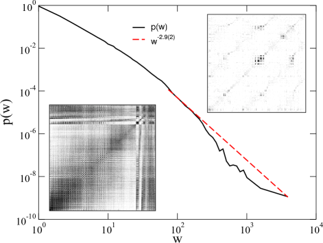
Figure 1: Weight distribution of the fruit-fly connectome. Right inset: adjacency matrix plot of the fruit-fly connectome. Left inset: full adjacency matrix down-sampled with a max pooling kernel of size $10\times 10$. Black dots denote connections between presynaptic and postsynaptic neurons. Right inset: zoom-in to the center of the matrix without down-sampling.

The modularity quotient of the FF network defined by

$$Q=\frac{1}{N\langle{k}\rangle}\sum\limits_{ij}\left(A_{ij}-\frac{k_{i}k_{j}}{N\langle{k}\rangle}\right)\delta(g_{i},g_{j}),$$ (1)

is very low: $Q=0.002264$, where $A_{ij}$ is the adjacency matrix and $\delta(i,j)$ is the Kronecker delta function. The weighted modularity quotient is even lower: $Q_{w}=0.0001184$. In comparison, the modularity quotient of the KKI-18 network is about $40$ times greater: $Q_{w}=0.0047$

The Watts-Strogatz clustering coefficient Watts and Strogatz (1998) of a network of $N$ nodes is

$$C=\frac{1}{N}\sum_{i}2n_{i}/[k_{i}(k_{i}-1)]\ ,$$ (2)

where $n_{i}$ denotes the number of direct edges interconnecting the $k_{i}$ nearest neighbors of node $i$. This is $C_{FF}=0.191$, about $12.36$ times larger than that of a random network of same size: $C_{r}=0.01545$, obtained by $C_{r}=\langle k\rangle/N$. In case of KKI-18 we found: $C_{KKI-18}=0.5$.

The average shortest path length is defined as

$$L=\frac{1}{N(N-1)}\sum_{j\neq i}d(i,j)\ ,$$ (3)

where $d(i,j)$ is the graph distance between vertices $i$ and $j$. For FF this is $L_{FF}=2.7531$, about $1.3$ times larger than that of the random network of same size: $L_{r}=2.1162$, following from the formula Fronczak et al. (2004):

$$L_{r}=\frac{\ln(N)-0.5772}{\ln\langle k\rangle}+1/2\ .$$ (4)

So, the FF is a small-world network, according to the definition of the coefficient Humphries and Gurney (2008):

$$\sigma=\frac{C/C_{r}}{L/L_{r}}\ ,$$ (5)

because $\sigma_{FF}=9.5$ is much larger than unity.

We estimated the effective graph (topological) dimension, which is obtained by the breadth-first search algorithm: $d=5.4(5)$, which is defined by $N(r)\sim r^{d}$, where we counted the number of nodes $N(r)$ with chemical distance $r$ or less from the seeds and calculated averages over the trials. Note, however that finite size cutoff happens already for $r>2$. This dimension renders this model into the mean-field region, because the upper-critical dimension is $d_{c}=4$.

III Numerical analysis of the Kuramoto model

We used the KM of interacting oscillators Kuramoto (2012) to study the synchronization on the human KKI-18, the FF connectome as well as on ER random graphs for comparison KM was originally defined on full graphs, corresponding to mean-field behavior Hong et al. (2007). The critical dynamical behavior has recently been explored on various random graphs Choi et al. (2013); Juhász et al. (2019); Ódor and Kelling (2019). Phase transition in the KM can happen only above the lower critical dimension $d_{c}^{-}=4$ HPClett. In lower dimensions, a true, singular phase transition in the $N\to\infty$ limit is not possible, but partial synchronization can emerge with a smooth crossover if the oscillators are strongly coupled.

The KM describes interacting oscillators with phases $\theta_{i}(t)$ located at $N$ nodes of a network, which evolve according to the dynamical equation

$$\dot{\theta_{i}}(t)=\omega_{i,0}+K\sum_{j}W_{ij}\sin[\theta_{j}(t)-\theta_{i}(t)].$$ (6)

Here, $W_{ij}$ is the weighted adjacency matrix and summation is performed over neighboring nodes of $i$. There is a quenched heterogeneity in $W_{ij}$ as well as in $\omega_{i,0}$, which is the intrinsic frequency of the $i$-th oscillator, drawn from a $g(\omega_{i,0})$ distribution. The global coupling $K$ is the control parameter of the model by which we can tune the system between asynchronous and synchronous states. One usually follows the synchronization transition through studying the Kuramoto order parameter defined by

$$R(t)=\frac{1}{N}\left|\sum_{j=1}^{N}e^{i\theta_{j}(t)}\right|,$$ (7)

which is non-zero above a critical coupling strength $K>K_{c}$ or tends to zero for $K<K_{c}$ as $R\propto\sqrt{1/N}$. At $K_{c}$, $R$ exhibits growth as

$$R(t,N)=N^{-1/2}\,t^{\eta}\,f_{\uparrow}(t/N^{\tilde{z}})\ ,$$ (8)

with the dynamical exponents ${\tilde{z}}$ and $\eta$, if the initial state is incoherent.

Additionally, we have also calculated another order parameter, which measures the spread of frequencies

$$\Omega(t,N)=\frac{1}{N}\sum_{j=1}^{N}(\overline{\omega}-\omega_{j})^{2},$$ (9)

In case of a single peaked self-frequency distribution it is an appropriate order-parameter, besides the more commonly used measure, which counts the number of oscillators in the largest cluster having an identical frequency Hong et al. (2005).

Generally we used the Runge-Kutta-4 integration algorithm with step sizes $\delta=0.01$ or $\delta=0.1$ if it was sufficient, via a special, parallel algorithm, running on GPU-s. We have averaged over the solutions for thousands of different initial self-frequencies, chosen randomly from Gaussian distributions with zero mean and unit variance at each control parameter value. In a previous paper Ódor et al. (2021), we have shown the possibility of rescaling these onto more realistic, narrow banded frequencies thanks to the Galilean invariance of the KM. Some of the runs, especially for larger couplings $K\geq 3$ , were tested by the adaptive solver Bulrisch-Stoer P. (1983) of the boost library. For very large couplings, $K>30$ only the adaptive solver could provide reasonable results.

First we have determined the growth behavior of $R(t)$ of the Kuramoto equation solution with incoming weight normalization, in order to mimic a local homeostasis, provided by the unknown balance of inhibition/excitation:

$$W^{\prime}_{ij}=W_{ij}/\sum_{j\;\in\;\rm{neighb.\ of}\ i}W_{ij}.$$ (10)

This renormalization has been used in previous connectome studies  Ódor (2016); Ódor and Kelling (2019); Ódor et al. (2021); Rocha et al. (2018); Ódor et al. (2021). Recently, a comparison of modeling and experiments arrived at a similar conclusion: equalized network sensitivity improves the predictive power of a model at criticality in agreement with the fMRI correlations Rocha et al. (2018). The solution of equations were started from incoherent states, but for larger $K$ values it was better to start from coherent states in order to reach the steady states without large oscillations.

As Fig. 2 shows there is a transient region up to $t<30$ followed by a level-off as the correlation length exceeds the system size, causing a steady state saturation of the phase synchronization. In the transient region curves with $K>1.7$ exhibit an upward, while those with $K<1.7$ downward curvature. To see the corrections to scaling we determined the effective exponents of $R$ as the discretized, logarithmic derivative of Eq. (8) at these discrete time steps $t_{k}$, near the transition point

$$\eta_{\mathrm{eff}}=\frac{\ln\langle R(t_{k+3})\rangle-\ln\langle R(t_{k})\rangle}{\ln(t_{k+3})-\ln(t_{k})}\ .$$ (11)

Here the brackets denote sample averaging over different initial conditions. These effective exponent values can be seen on the local slope inset of the figure. Some fluctuation and modulation effects, coming from the weak modular graph structure of the FF, remain. One can estimate a synchronization transition at $K_{c}=1.70(2)$, characterized by $\eta=0.70(5)$. This is close to the mean-field value, obtained in Choi et al. (2013); Ódor and Kelling (2019) $\eta_{MF}\simeq 0.75$ and higher than those of the large human white matter connectomes, where the graph dimension was found to be $d<d_{c}=4$ Gastner and Ódor (2016).

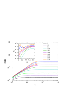
Figure 2: Growth of $R(t)$ on the weight normalized FF, using incoherent initial state for different $K$ global coupling values as shown by the legends. One can locate a transition by the convex/concave criterion at $K_{c}=1.70(2)$, where an initial PL growth can be observed. The inset shows the local slopes of the same data on $1/t$ scale with the same color coding from $K=1.75$ (top curve) to $K=1.55$ (bottom curve).

Using the steady state values we also determined the transition as the function of the control parameter $K$. Fig. 3 displays a comparison of the FF transition with the results obtained on the KKI-18 human connectome. The transition is sharp around $K_{c}=1.70(2)$ and $R$ changes from $0.02$ to $0.97$ as $K$ from $1.2$ to $6$. In comparison, similar change of $R$ for the KKI-18 spans from $1.6<K<10^{3}$. We also plotted the results obtained without the application of weight normalization by running on the raw FF network on Fig.3. In this case the transition occurs at a much lower coupling: $K_{c}=0.00090(5)$, so we multiplied them on the plot by the average weight value $K^{\prime}=K\times 628$. Note, that the transition of the raw case is not smoother than the homeostatic one, just it appears to be like that, as the consequence of the linear up-scaling of $K$. It happens in the $0.0005<K<0.2$ region. The steady state results on a random ER graph with $N=22.000$ and $\langle k\rangle=315$ are also displayed. Here we used weight normalization condition (10) as for FF. The synchronization transition occurs in the $1.4<K<5$ region, which is slightly narrower than for the FF.

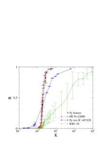
Figure 3: Synchronization transition of $R(t\to\infty,K)$ on different graphs.

We can analyze the transition further by determining the fluctuations of $R(t\to\infty,K)$ near the transition. This is plotted on Fig. 4. As we can see the standard deviation: $\sigma(R(t\to\infty,K))$ of the FF is very similar to that of an ER graph of same size and average degree, but somewhat wider. In comparison the KKI-18 exhibits a much more smeared transition region, even though the weighted average degree is smaller: $\langle w\rangle_{\mathrm{KKI-18}}=448$ than that of the fly connectome: $\langle w\rangle_{\mathrm{FF}}=628$. As $d_{KKI-18}<d_{c}^{-}=4$ this is a crossover transition and no exact finite scaling is applicable to rescale it.

In case of KM on random ER graphs increasing the size causes small decrease of $K_{c}$ as well as narrower peaks as shown in Ódor and Kelling (2019). If we increase the average degree from $\langle k\rangle=4$ to $\langle k\rangle=350$, the critical point $K_{c}\simeq 0.482$ moves to $K_{c}\simeq 1.65$ close to that of the full graph case $K_{c}\simeq 1.6$. Thus, one may expect that the bigger average degree of FF would cause a peak at larger couplings.

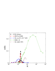
Figure 4: Fluctuations of $R(t\to\infty,K)$ for different graphs.

In contrary we can see that the Hierarchical Modular Network (HMN) structure of KKI-18 causes nontrivial effects on the $\sigma(R)$ peak and on the width of the phase synchronization transition region.

We have also investigated the frequency synchronization order parameter, which is defined here as Eq.( 9). In case of the single peaked Gaussian self-frequencies one can follow the frequency entrainment by this quantity. This has the advantage of having lower critical dimension: $d_{c}^{-}=2$ as compared to the phases: $d_{c}^{-}=4$. This was showed on regular lattices HPClett, but Ref. Millán et al. (2019) obtained similar conclusion on complex network. Thus in case of graph, like the KKI-18, a real frequency phase-transition can occur, if we found the the human brain to exhibit topological dimension $d>2$, even for higher resolutions.

Indeed as the Fig. 5 shows the frequency transitions on the fly on the ER and on the human KKI-18 are very similar. Now the finite size scaling

$$|K-K_{c}|\propto N^{-1/\tilde{\nu}}$$ (12)

is applicable as all of these graphs have $d>d_{c}^{-}$.

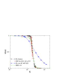
Figure 5: Frequency entrainment order parameter $\Omega(t\to\infty,K)$ of the KM obtained on different graphs.

By considering the fluctuations of this order parameter: $\sigma(\Omega(t\to\infty,K))$ we find that the peaks are close, but the KKI-18 transition region is much wider in the high coupling region, than in case of the ER and the FF (see  6).

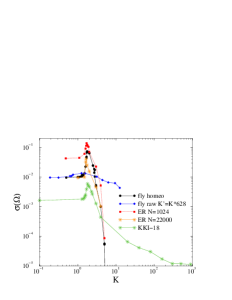
Figure 6: Fluctuations of the frequency entrainment order parameter $\sigma(\Omega(t\to\infty,K))$ for different graphs.

The fluctuation region on the random ER graph is the narrowest and the peak value decreases as we increase $N$. We have also plotted the results obtained on the raw FF graph, up-scaled by the average value of the weights: $K^{\prime}=K\times 628$. The distribution looks wider, but this is just the consequence of the horizontal rescaling.

Finally, we also performed measurements for the desynchronization times as in Ódor and Kelling (2019); Ódor et al. (2021). To define desynchronization ”avalanches” in terms of the Kuramoto order parameter, we can consider processes, starting from fully de-synchronized initial states by a single phase perturbation (or by an external phase shift at a node), followed by growth and return to $R(t_{x})=1/\sqrt{N}$, corresponding to the disordered state of $N$ oscillators. In the simulations one can measure the first return, crossing times $t_{x}$ in many random realizations of the system. In  Ódor and Kelling (2019); Ódor et al. (2021), the return or spontaneous desynchronization time was estimated by $t_{x}=(t_{k}+t_{k-1})/2$, where $t_{k}$ was the first measured crossing time, when $R(t_{k})$ fell below $1/\sqrt{N}$.

Following a histogramming procedure, one can obtain $p_{x}(t)$ distributions shown on Fig.7 for the weight normalized, homeostatic case. For $K=1.65(5)$ (i.e. near the transition point estimated before), we can find critical PL decay characterized by $\tau_{t}\simeq 1.6(1)$, close to the mean-field value of the spontaneous desynchronization of $R(t)$, as defined in Ódor and Kelling (2019).

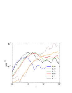
Figure 7: Desynchronization time distributions $p_{x}(t)t^{1.6}$ near the transition point in case of the fly connectome with local homeostasis for different couplings, as shown by the legends.

For $K>1.7$ the curves decay as $p_{x}(t)\sim 1/t$ up to a cutoff, corresponding to the ordered state, while for $K<1.5$ the curves break down sharply. It is hard to decide if there is a narrow GP in the $1.5\leq K\leq 1.7$ region due to the strong fluctuations remained even after averaging over tens of thousands of samples with different $\omega_{i,0}$ initial conditions.

Similar results have been obtained using the raw FF graph, as shown on Fig.8. The transition point is at $K_{c}=0.0008(1)$, where we can observe a saturation of the $p_{x}(t)t^{1.6}$ for $t>200$, thus again mean-field scaling occurs. At $K=0.001$ we can also see the $p_{x}(t)\propto 1/t$ decay, corresponding to the synchronized state, in which arbitrarily large decay times can happen, but no signs of sub-critical PL-s, corresponding to a GP have been found.

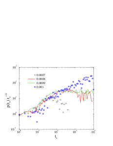
Figure 8: Desynchronization time distributions $p_{x}(t)t^{1.6}$ near the transition point, using the raw fly connectome graph for different couplings, as shown by the legends.

For comparison we have done this analysis for full and for ER graphs with $N=22.000$ and $\langle k\rangle=315$. Now we just show the results for the ER case on Fig.9. Below $K_{c}\simeq 1.59$ the $p_{x}(t)t^{1.6}$ curves break down quickly, without any sign of PL tails. While for $K=1.59$ we see a saturation for $t>200$, the $K=1.62$ curve seems to cross over to the singular $p_{x}(t)\sim 1/t$ behavior. Going beyond this the curves break down very quickly again, suggesting that within the maximum measurement time $t=10^{4}$ desynchronization events could not happen.

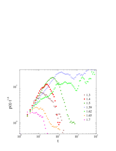
Figure 9: Desynchronization time distributions $p_{x}(t)t^{1.6}$ near the transition point in case of ER graphs with different couplings, as shown by the legends.

We have also tested the effects of the introduction of negative couplings by flipping the sign of outgoing weight values: $W_{ij}=-W_{ij}$ of $30\%$ of randomly chosen nodes. As the consequence the transition region broadens considerably as shown on Fig.4.

IV Conclusions

In conclusion we have investigated KM at the edge of synchronization by comparing the dynamical behavior on the FF, ER and the KKI-18 large human connectome. The FF network topology is rather similar, almost free of modules, to the high-dimensional ER graph. Thus we found a mean-field like behavior, unlike for the KKI-18, which has $d<4$, a HMN structure, which enhances and broadens the transition region with the appearance of GP singularity. Although the link weight distribution of FF exhibits a fat tail, it does not seem to be enough to introduce visible GP effects, or maybe a very weak ones. Thus one can think that the fly brain’s simpler structure does not allow the appearance of the complex sub-critical dynamical phenomena, which are present in the human brain. The lack of modules on smaller scales may also explain that in global human brain measurements non- universal scaling Palva et al. (2013) are reported, while local electrode studies Beggs and Plenz (2003) show mean-field exponents. Possibly electrode studies Beggs and Plenz (2003) measure local activity and within those small volumes modules and GP are less relevant than on the whole brain scale.

The range of the synchronization transition region is slightly broader than in case of the ER, but much narrower than in case of the KKI-18 when we applied link weight normalization, to mimic local homeostasis. This is shown both by the phase and frequency order parameters. Without link weight normalization the KM transition occurs at very low coupling values, but shows mean-field scaling. This was shown by measuring the synchronization growth exponent $\eta$ and the desynchronization time exponent $\tau_{t}$.

If we allow negative couplings the transition region broadens further, leading to a spin glass like phase, where GP effects may also emerge. But as the details and dynamics of such negative couplings are unknown in case of the FF-s we have not investigated this further. We have arrived to similar conclusions as the very recent publication by Buendia et al Buendia et al. (2021) in case of the complex interplay between structure and dynamics, but we showed the emergence of a critical transition in terms of desynchronization times as well as the initial-slip, characterized by the exponent $\eta$.

Given the limitations and assumptions we mentioned in the Introduction we have provided ample numerical evidence for the different dynamical critical behavior of the Kuramoto model, as the result of the different connectome topology of a fly and of a human brain. Further studies on other animals, preferably mammals should be performed in order to fully justify the proposition expressed in the title.

References

- Beggs and Plenz (2003) J. Beggs and D. Plenz, J. Neuroscience 23, 11167 (2003).
- Mazzoni et al. (2007) A. Mazzoni, F. D. Broccard, E. Garcia-Perez, P. Bonifazi, M. E. Ruaro, and V. Torre, PLOS ONE 2, 1 (2007).
- Pasquale et al. (2008) V. Pasquale, P. Massobrio, L. Bologna, M. Chiappalone, and S. Martinoia, Neuroscience 153, 1354 (2008).
- Friedman et al. (2012) N. Friedman, S. Ito, B. A. W. Brinkman, M. Shimono, R. E. L. DeVille, K. A. Dahmen, J. M. Beggs, and T. C. Butler, Phys. Rev. Lett. 108, 208102 (2012).
- Hahn et al. (2010) G. Hahn, T. Petermann, M. N. Havenith, S. Yu, W. Singer, D. Plenz, and D. Nikolić, Journal of Neurophysiology 104, 3312 (2010), pMID: 20631221.
- Shriki et al. (2013) O. Shriki, J. Alstott, F. Carver, T. Holroyd, R. N. Henson, M. L. Smith, R. Coppola, E. Bullmore, and D. Plenz, Journal of Neuroscience 33, 7079 (2013).
- Tagliazucchi et al. (2012) E. Tagliazucchi, P. Balenzuela, D. Fraiman, and D. Chialvo, Frontiers in Physiology 3, 15 (2012).
- Scott et al. (2014) G. Scott, E. D. Fagerholm, H. Mutoh, R. Leech, D. J. Sharp, W. L. Shew, and T. Knöpfel, Journal of Neuroscience 34, 16611 (2014).
- Priesemann et al. (2014) V. Priesemann, M. Wibral, M. Valderrama, R. Pröpper, M. Le Van Quyen, T. Geisel, J. Triesch, D. Nikolić, and M. H. J. Munk, Frontiers in Systems Neuroscience 8, 108 (2014).
- Bellay et al. (2015) T. Bellay, A. Klaus, S. Seshadri, and D. Plenz, Elife 4, e07224 (2015).
- Hahn et al. (2017) G. Hahn, A. Ponce-Alvarez, C. Monier, G. Benvenuti, A. Kumar, F. Chavane, G. Deco, and Y. Frégnac, PLOS Computational Biology 13, 1 (2017).
- Seshadri et al. (2018) S. Seshadri, A. Klaus, D. Winkowski, and et al., Transl Psychiatry 8 (2018).
- Palva et al. (2013) J. Palva, A. Zhigalov, J. Hirvonen, O. Korhonen, K. Linkenkaer-Hansen, and S. Palva, Proceedings of the National Academy of Sciences of the United States of America 110, 3585 (2013).
- Chialvo and Bak (1999) D. Chialvo and P. Bak, Neuroscience 90, 1137 (1999).
- Chialvo (2004) D. R. Chialvo, Physica A: Statistical Mechanics and its Applications 340, 756 (2004), complexity and Criticality: in memory of Per Bak (1947–2002).
- Chialvo (2006) D. R. Chialvo, Nature Physics 2, 301 (2006).
- Chialvo (2007) D. R. Chialvo, AIP Conference Proceedings 887, 1 (2007), eprint https://aip.scitation.org/doi/pdf/10.1063/1.2709580.
- Chialvo et al. (2008) D. R. Chialvo, P. Balenzuela, and D. Fraiman, AIP Conference Proceedings 1028, 28 (2008), eprint https://aip.scitation.org/doi/pdf/10.1063/1.2965095.
- Fraiman et al. (2009) D. Fraiman, P. Balenzuela, J. Foss, and D. R. Chialvo, Phys. Rev. E 79, 061922 (2009).
- Expert et al. (2011) P. Expert, R. Lambiotte, D. R. Chialvo, K. Christensen, H. J. Jensen, D. J. Sharp, and F. Turkheimer, Journal of The Royal Society Interface 8, 472 (2011).
- Fraiman and Chialvo (2012) D. Fraiman and D. Chialvo, Frontiers in Physiology 3, 307 (2012).
- Deco and Jirsa (2012) G. Deco and V. K. Jirsa, Journal of Neuroscience 32, 3366 (2012).
- Deco et al. (2014) G. Deco, A. Ponce-Alvarez, P. Hagmann, G. Romani, D. Mantini, and M. Corbetta, Journal of Neuroscience 34, 7886 (2014).
- Senden et al. (2017) M. Senden, N. Reuter, M. P. van den Heuvel, R. Goebel, and G. Deco, NeuroImage 146, 561 (2017).
- Muñoz (2018) M. A. Muñoz, Rev. Mod. Phys. 90, 031001 (2018).
- Haimovici et al. (2013) A. Haimovici, E. Tagliazucchi, P. Balenzuela, and D. R. Chialvo, Phys. Rev. Lett. 110, 178101 (2013).
- Johnson S. and Marro (2013) J. J. Johnson S., Torres and J. Marro, PLoS ONE 8, e50276 (2013).
- Bak et al. (1987) P. Bak, C. Tang, and K. Wiesenfeld, Phys. Rev. Lett. 59, 381 (1987).
- Chialvo (2010) D. R. Chialvo, Nature Physics 6, 744 (2010).
- Touboul and Destexhe (2017) J. Touboul and A. Destexhe, Phys. Rev. E 95, 012413 (2017), URL https://link.aps.org/doi/10.1103/PhysRevE.95.012413.
- Vojta (2006) T. Vojta, Journal of Physics A: Mathematical and General 39, R143 (2006).
- Griffiths (1969) R. B. Griffiths, Phys. Rev. Lett. 23, 17 (1969).
- Ódor (2014) G. Ódor, Phys. Rev. E 89, 042102 (2014).
- Karsai et al. (2018) M. Karsai, H.-H. Jo, and K. Kaski, SpringerBriefs in Complexity (2018).
- Cota et al. (2016) W. Cota, S. C. Ferreira, and G. Ódor, Phys. Rev. E 93, 032322 (2016).
- Muñoz et al. (2010) M. A. Muñoz, R. Juhász, C. Castellano, and G. Ódor, Phys. Rev. Lett. 105, 128701 (2010).
- Ódor et al. (2015) G. Ódor, R. Dickman, and G. Ódor, Scientific Reports 5, 14451 (2015).
- Cota et al. (2018) W. Cota, G. Ódor, and S. C. Ferreira, Scientific Reports 8, 9144 (2018).
- Gastner and Ódor (2016) M. T. Gastner and G. Ódor, Scientific Reports 6, 27249 (2016).
- Ódor (2016) G. Ódor, Phys. Rev. E 94, 062411 (2016).
- Ódor et al. (2021) G. Ódor, M. T. Gastner, J. Kelling, and G. Deco, Journal of Physics: Complexity 2, 045002 (2021).
- Sporns et al. (2005) O. Sporns, G. Tononi, and R. Kötter, PLOS Computational Biology 1, e42 (2005).
- Scheffer and Meinertzhagen (2019) L. K. Scheffer and I. A. Meinertzhagen, Annual Review of Cell and Developmental Biology 35, 637 (2019), pMID: 31283380, eprint https://doi.org/10.1146/annurev-cellbio-100818-125444.
- Xu et al. (2020) C. S. Xu, M. Januszewski, Z. Lu, S.-y. Takemura, K. J. Hayworth, G. Huang, K. Shinomiya, J. Maitin-Shepard, D. Ackerman, S. Berg, et al., bioRxiv (2020).
- Penn et al. (2016) Y. Penn, M. Segal, and E. Moses, Proceedings of the National Academy of Sciences of the United States of America 113, 3341 (2016).
- Di Santo et al. (2018) S. Di Santo, P. Villegas, R. Burioni, and M. Muñoz, Proceedings of the National Academy of Sciences of the United States of America 115, E1356 (2018).
- Kuramoto (2012) Y. Kuramoto, Chemical Oscillations, Waves, and Turbulence, Springer Series in Synergetics (Springer Berlin Heidelberg, 2012), ISBN 9783642696893.
- Villegas et al. (2014) P. Villegas, P. Moretti, and M. Muñoz, Scientific Reports 4 (2014).
- Villegas et al. (2016) P. Villegas, J. Hidalgo, P. Moretti, and M. Muñoz (2016), pp. 69–80.
- Millán et al. (2018) A. Millán, J. Torres, and G. Bianconi, Scientific Reports 8 (2018).
- Ódor and Kelling (2019) G. Ódor and J. Kelling, Scientific Reports 9, 19621 (2019).
- Ódor et al. (2021) G. Ódor, J. Kelling, and G. Deco, J. Neurocomputing 461, 696 (2021).
- Delettre et al. (2019) C. Delettre, A. Messé, L.-A. Dell, O. Foubet, K. Heuer, B. Larrat, S. Meriaux, J.-F. Mangin, I. Reillo, C. de Juan Romero, et al., Network Neuroscience 3, 1038 (2019).
- Abrams and Strogatz (2004) D. M. Abrams and S. H. Strogatz, Phys. Rev. Lett. 93, 174102 (2004).
- Fosque et al. (2021) L. J. Fosque, R. V. Williams-García, J. M. Beggs, and G. Ortiz, Phys. Rev. Lett. 126, 098101 (2021).
- dow (2020) The hemibrain dataset (v1.0.1) (2020), URL https://storage.cloud.google.com/hemibrain-release/neuprint/hemibrain_v1.0.1_neo4j_inputs.zip.
- Scheffer (2020) L. K. Scheffer, Graph properties of the adult drosophila central brain (2020), URL https://www.biorxiv.org/content/early/2020/05/20/2020.05.18.102061.
- Watts and Strogatz (1998) D. J. Watts and S. H. Strogatz, Nature 393, 440 (1998).
- Fronczak et al. (2004) A. Fronczak, P. Fronczak, and J. A. Hołyst, Physical Review E 70, 056110 (2004).
- Humphries and Gurney (2008) M. D. Humphries and K. Gurney, PLOS ONE 3, e0002051 (2008).
- Hong et al. (2007) H. Hong, H. Chaté, H. Park, and L.-H. Tang, Physical Review Letters 99 (2007).
- Choi et al. (2013) C. Choi, M. Ha, and B. Kahng, Physical Review E - Statistical, Nonlinear, and Soft Matter Physics 88 (2013).
- Juhász et al. (2019) R. Juhász, J. Kelling, and G. Ódor, Journal of Statistical Mechanics: Theory and Experiment 2019, 053403 (2019).
- Hong et al. (2005) H. Hong, H. Park, and M. Choi, Physical Review E - Statistical, Nonlinear, and Soft Matter Physics 72 (2005).
- P. (1983) D. P., Numerische Mathematik 41, 399 (1983).
- Rocha et al. (2018) R. Rocha, L. Koçillari, S. Suweis, M. Corbetta, and A. Maritan, Scientific Reports 8 (2018).
- Millán et al. (2019) A. P. Millán, J. J. Torres, and G. Bianconi, Phys. Rev. E 99, 022307 (2019), URL https://link.aps.org/doi/10.1103/PhysRevE.99.022307.
- Buendia et al. (2021) V. Buendia, P. Villegas, R. Burioni, and M. A. Munoz, The broad edge of synchronisation: Griffiths effects and collective phenomena in brain networks (2021), eprint 2109.11783.