A note on explicit solutions of FitzHugh-Rinzel system

Abstract

The numerous scientific feedbacks that the FitzHugh-Rinzel system (FHR) is having in various scientific fields, lead to further studies on the determination of its explicit solutions. Indeed, such a study can help to get a better understanding of several behaviours in the complex dynamics of biological systems. In this note, a class of travelling wave solutions is determined and specific solutions are achieved to explicitly show the contribution due to a diffusion term considered in the FHR model.

1 Introduction

One of the most commonly known models in biomathematics is the FitzHugh-Rinzel (FHR) system [1, 2, 3]. It derives from the FitzHugh-Nagumo (FHN) model [4, 11, 5, 6, 10, 12, 8, 9, 7] and unlike the latter, it has an additional variable suitable for evaluating and studying nerve cell bursting phenomena.

In general, bursting oscillations can be described by a system variable that changes periodically from a rapid spike oscillation to a silent phase during which the membrane potential changes slowly [13].

Studies concerning bursting phenomena are increasingly present in various scientific fields (see, for instance, [14] and references therein), and in particular, some applications concern the restoration of synaptic connections. In fact, it seems that certain nanoscale memristor devices have the potential to reproduce the behaviour of a biological synapse, suggesting that in the future electronic synapses may be introduced to directly connect neurons [15, 16].

The interest aroused the FHR system applications also leads to the research of explicit solutions. Indeed, in an attempt to understand the various phenomena that the FitzHugh-Rinzel system is able to describe, knowing the expression of the solution can lead to a more complete analysis of the phenomenon itself. In view of this, in this paper, the exact solutions are determined by pointing the research to travelling wave solutions.

The paper is organized as follows. In Section 2, the mathematical problem is defined. In Section 3, taking into account travelling waves, a class of explicit solutions is determined, and in Section 4, a solution has been developed to show the incidence of the diffusive term inserted in the FHR system. Finally, in Section 5, some concluding remarks have been underlined.

2 Mathematical Considerations

Generally, the FitzHugh-Rinzel model under consideration is the following:

(2.1) $$\left\{\begin{array}[]{lll}\displaystyle{\frac{\partial\,u}{\partial\,t}}=\,u-u^{3}/3+I\,-\,w\,\,+y\\ \\ \displaystyle{\frac{\partial\,w}{\partial\,t}}\,=\,\varepsilon(-\beta w+c+u)\\ \\ \displaystyle{\frac{\partial\,y}{\partial\,t}}\,=\,\delta(-u+h-dy),\end{array}\right.$$

where $I,\varepsilon,\beta,c,d,h,\delta$ indicate arbitrary constants.

In this paper, in order to evaluate also the contribution due to a diffusion term, the following FHR system is considered:

(2.2) $$\left\{\begin{array}[]{lll}\displaystyle{\frac{\partial\,u}{\partial\,t}}=\,D\,\frac{\partial^{2}\,u}{\partial\,x^{2}}-au\,\,+ku^{2}\,(\,a+1\,-u\,)\,-\,w\,\,+y\,\,+I\\ \\ \displaystyle{\frac{\partial\,w}{\partial\,t}}\,=\,\varepsilon(-\beta w+c+u)\\ \\ \displaystyle{\frac{\partial\,y}{\partial\,t}}\,=\,\delta(-u+h-dy).\end{array}\right.$$

Indeed, the term with $D>0$ represents just the diffusion contribution and it derives from the Hodgkin-Huxley (HH) theory for nerve membranes when the spatial variation in the potential $V$is considered [11].

When $D=0,$ $k=1/3$ and $a=-1,$ system (2.2) turns into (2.1).

After indicating by means of

(2.3) $$u(x,0)\,=\,u_{0}\,,\qquad w(x,0)\,=\,w_{0}\qquad y(x,0)=y_{0},\qquad\qquad(\,x\,\in\Re\,)$$

the initial values, from (2.2) it follows that:

(2.4) $$\left\{\begin{array}[]{lll}\displaystyle w\,=\,w_{0}\,e^{\,-\,\varepsilon\beta\,t\,}\,+\,\frac{c}{\beta}\,(1-e^{-\,\varepsilon\,\beta\,t})\,+\varepsilon\int_{0}^{t}\,e^{\,-\,\varepsilon\,\beta\,(\,t-\tau\,)}\,u(x,\tau)\,d\tau\\ \\ \displaystyle y\,=\,y_{0}\,e^{\,-\,\delta\,d\,t\,}\,+\,\frac{h}{d}\,(1-e^{-\,\delta\,d\,t})\,-\delta\int_{0}^{t}\,e^{\,-\,\delta\,d\,(\,t-\tau\,)}\,u(x,\tau)\,d\tau.\end{array}\right.$$

So, when $k=1,$ problem (2.2) turns into

(2.5) $$\left\{\begin{array}[]{lll}\displaystyle u_{t}-Du_{xx}+au+\int^{t}_{0}[\varepsilon e^{-\varepsilon\beta(t-\tau)}+\delta e^{-\delta d(t-\tau)}]u(x,\tau)d\tau=F(x,t,u)\\ \\ \displaystyle\,u(x,0)\,=u_{0}(x)\,\,\,\,\,\,x\,\in\,\Re,\end{array}\right.$$

where

(2.6) $$F=u^{2}(a+1-u)+I-w_{0}e^{-\varepsilon\beta t}+y_{0}e^{-\delta dt}-\frac{c}{\beta}(1-e^{-\varepsilon\beta t})+\frac{h}{d}(1-e^{-\delta dt}).$$

By means of the Laplace transform, the solution of problem (2.5)-(2.6) can be expressed through an integral equation involving the fundamental solution $H(x,t).$ Indeed, in [14] it has been proved that the solution assumes the following form:

$$\displaystyle u(x,t)=\int_{\Re}\,H(x-\xi,t)\,\,u_{0}(\xi)\,\,d\xi\,$$

(2.7)

$$\displaystyle\,+\,\int^{t}_{0}d\tau\int_{\Re}H(x-\xi,t-\tau)\,\,F\,[\,\xi,\tau,u(\xi,\tau\,)\,]\,\,d\xi.$$

Denoting by $J_{1}(z)\,$ the Bessel function of first kind and order $\,1,\,$ and considering the following functions:

$$H_{1}(x,t)\,=\,\,\,\frac{e^{-\frac{x^{2}}{4\,D\,t}\,}}{2\sqrt{\pi Dt}}\,\,\,e^{-\,a\,t}\,+\,$$

(2.8)

$$\displaystyle-\frac{1}{2}\,\,\,\,\,\int^{t}_{0}\frac{e^{-\frac{x^{2}}{4\,D\,y}\,-a\,y}}{\sqrt{t-y}}\,\,\,\frac{\,\sqrt{\varepsilon}\,\,e^{-\beta\varepsilon\,(\,t\,-\,y\,)}}{\sqrt{\pi\,D\,}}J_{1}(\,2\,\sqrt{\,\varepsilon\,y\,(t-y)\,}\,\,)\,\,\}dy,$$

(2.9) $$H_{2}=\int_{0}^{t}H_{1}(x,y)\,\,e^{-\delta d(t-y)}\sqrt{\frac{\delta y}{t-y}}J_{1}(\,2\,\sqrt{\,\delta\,y\,(t-y)\,}\,\,\,dy,$$

one gets

(2.10) $$H=H_{1}-H_{2}.$$

3 Explicit Solutions

Several methods have been developed to find exact solutions of the partial differential equations [19, 17, 20, 21, 18, 22].

Here, in order to find explicit solutions in the form of travelling solutions, from system (2.2) the following equation is deduced:

(3.11) $$u_{tt}=Du_{xxt}-au_{t}+2uu_{t}(a+1)-3u^{2}u_{t}+\varepsilon\beta w-\varepsilon c-\varepsilon u-\delta u+\delta h-\delta dy.$$

Moreover, letting

$\beta\varepsilon=\delta d,$

one obtains

$$u_{tt}=Du_{xxt}-au_{t}+2uu_{t}(a+1)-3u^{2}u_{t}-\varepsilon c-\varepsilon u-\delta u+\delta h+$$

$$\varepsilon\beta(-u_{t}+Du_{xx}-au+u^{2}(a+1)-u^{3}+I).$$

Now, if one introduces the variable wave

$$z=x-C\,t,$$

from (3) one gets

$$\displaystyle D\,C\,u_{zzz}+(C^{2}-\varepsilon\beta\,D)u_{zz}-3Cu^{2}u_{z}+2C(a+1)u\,u_{z}+\varepsilon\beta u^{3}+$$

(3.13)

$$\displaystyle-\,C\,(a\,+\varepsilon\beta)\,u_{z}-\,\varepsilon\beta(a+1)u^{2}+\,\varepsilon\beta\,a\,u+(\varepsilon+\delta)\,u-K=0.$$

where

$K=(\delta h-\varepsilon\,c)+\varepsilon\beta\,I.$

The solutions to be determined are of the type

(3.14) $$u(z)=A\,\,f(z)+\,b\,,$$

where one assumes

(3.15) $$f(z)=\frac{1}{1+e^{(z-z_{0})}}.$$

Since

$$f_{z}-f^{2}+f=0,$$

it results in:

$$\displaystyle u_{z}=\,A\,f^{2}(z)-A\,f$$

$$\displaystyle u_{zz}=2\,Af^{3}-3\,A\,f^{2}+Af$$

$$\displaystyle u_{zzz}=6Af^{4}(z)-12\,A\,f^{3}(z)+7Af^{2}-Af$$

$$u\,\displaystyle u_{z}=A^{2}\,f^{3}+(-A^{2}+Ab)f^{2}-Abf$$

$$u^{2}\,u_{z}=A^{3}f^{4}+(2A^{2}\,b\,-A^{3})f^{3}+(Ab^{2}-2A^{2}b)f^{2}-Ab^{2}f.$$

In order to satisfy equation (3), one has to assume

(3.16) $$A^{2}=2D$$

and

(3.17) $$\delta=-\varepsilon.$$

Moreover, under the assumption that

$C>\sqrt{3}/4\,\,\wedge\,D>0$

or

$\displaystyle C<-\sqrt{3}/4\,\wedge\,D>0$

or

$\displaystyle 0<D<\,\frac{1}{12}\,(3-\sqrt{3}\,\sqrt{3-16\,C^{2}}\,\,\wedge\,-\sqrt{3}/4\,<\,C\,<\sqrt{3}/4\,$

or

$\displaystyle D>\,\frac{1}{12}\,(3+\sqrt{3}\,\sqrt{3-16\,C^{2}}\,\,\wedge-\sqrt{3}/4\,<\,C\,<\sqrt{3}/4\,,$

constants $a,b,$ and $K$ must satisfy the following relationships:

$$\displaystyle b=\frac{1}{6\sqrt{2D}}\,\,\big{(}\sqrt{2}\,\,\sqrt{2C^{2}+6D^{2}-3D}\,+2C-6D+3\sqrt{2D}\big{)}$$

$$\displaystyle a=3\,b-\frac{C}{A}+\frac{3A}{2}-1$$

$$\displaystyle K=\varepsilon\beta b^{3}-\varepsilon\beta(a+1)b^{2}+[(\varepsilon+\delta)+\varepsilon\beta a]b.$$

4 Application

The previous analysis allows us to make some applications. Indeed, in order to point out the contribution of diffusion effects due to the second order term with the coefficient $D,$ let us assume, for instance, the following values:

$$\,C=1;\,\,\,z_{0}=0;\,\,\,\varepsilon\,\beta=0.1\,.$$

In this way, this results in:

(4.18) $$b=\frac{\sqrt{6D^{2}-3D+2}}{6\sqrt{D}}-\frac{\sqrt{D}}{\sqrt{2}}+\frac{1}{3\sqrt{2D}}+\frac{1}{2}$$

and consequently, one has

(4.19) $$u(z)=\,\frac{\sqrt{2D}}{1+e^{z}}\,\,+\,\,\frac{\sqrt{6D^{2}-3D+2}}{6\sqrt{D}}-\frac{\sqrt{D}}{\sqrt{2}}+\frac{1}{3\sqrt{2D}}+\frac{1}{2}$$

Plotting the graph of function (4.19), it is possible to note how the diffusion term influences the damping of the solution both when the coefficient $D$ is equal to or less than $1$ and when $D$ is greater than $1.$

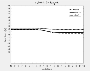
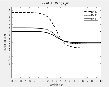
Figure 1: Solution u(z) when $\varepsilon\beta=0.1,$ $z_{0}=0$, $C=1.$ On the left: the values for the parameter D are such that $0<D\leq 1$, while in the right-hand graph: we have considered $D>1.$

5 Remarks

$\bullet$ The paper is concerned with the ternary autonomous dynamical system of FitzHugh-Rinzel (FHR) which, in biophysics, seems to be appropriate to describe some phenomena such as bursting oscillations. In this note, the FHR system under consideration includes a diffusion term, represented by a second order term, that derives directly from the Hodgkin-Huxley theory for nerve membranes and that is frequently inserted in the FitzHugh-Nagumo model, too.

$\bullet$ Solutions can be expressed by means of an integral equation involving the fundamental solution. However, to give direct feedbacks related to the contribution due to the diffusion term $D$, by means of the method of travelling wave, explicit solutions have been determined.

$\bullet$ Once arbitrary parameters have been set, the trajectories of solutions are shown, whether the parameter $D$ is less than $1$ or $D$ is greater than 1.

$\bullet$ Of course, as the chosen constants change, the behaviour of the various solutions can be pointed out.

References

- [1] N. A. Kudryashov. On Integrability of the FitzHugh – Rinzel Model. Russian Journal of Nonlinear Dynamics 15 (1) (2019) 13–19.
- [2] E. Kwessi and L. J. Edwards. A Nearly Exact Discretization Scheme for the FitzHugh–Nagumo Model. Differ Equ Dyn Syst. https://doi.org/10.1007/s12591-021-00569-5 (2021).
- [3] M. De Angelis. A priori estimates for solutions of FitzHugh-Rinzel system. https://arxiv.org/pdf/2106.09980.pdf (2021).
- [4] E M. Izhikevich. Dynamical Systems in Neuroscience: The Geometry of Excitability and Bursting. The MIT press, England, 2007.
- [5] M.De Angelis and P. Renno. Asymptotic effects of boundary perturbations in excitable systems, Discrete and continuous dynamical systems series B 19 (7) (2014) 2039-2045.
- [6] N. A. Kudryashov, K. R. Rybka and A. Sboev. Analytical properties of the perturbed FitzHugh-Nagumo model. Applied Mathematics Letters 76 (2018) 142-147.
- [7] M. De Angelis. On a model of superconductivity and biology. Advances and Applications in Mathematical Sciences 7 (1) (2010) 41-50.
- [8] S. Rionero and I. Torcicollo. On the dynamics of a nonlinear reaction–diffusion duopoly mode. International Journal of Non-Linear Mechanics 99 (2018) 105-111.
- [9] M. De Angelis. Asymptotic Estimates Related to an Integro Differential Equation. Nonlinear Dynamics and Systems Theory 13 (3) (2013) 217–228
- [10] M De Angelis. A priori estimates for excitable models. Meccanica 48 (10) (2013) 2491–2496.
- [11] J. D. Murray. Mathematical Biology I. Springer-Verlag, N.Y, 2003.
- [12] M. De Angelis and P. Renno. Existence, uniqueness and a priori estimates for a non linear integro - differential equation. Ricerche di Matematica 57 (2008) 95-109.
- [13] J. P. Keener and J. Sneyd. Mathematical Physiology . Springer-Verlag, N.Y, 1998.
- [14] F.De Angelis and M. De Angelis. On solutions to a FitzHugh–Rinzel type model. Ricerche di Matematica 70 (2021) 51–65.
- [15] Sung Hyun Jo, Ting Chang, Idongesit Ebong, Bhavitavya B. Bhadviya, Pinaki Mazumder, and Wei Lu. Nano Letters 10 (4) (2010) 1297-1301.
- [16] F. Corinto, V. Lanza, A. Ascoli and M. Gilli. Synchronization in Networks of FitzHugh-Nagumo Neurons with Memristor Synapses. 20th European Conference on Circuit Theory and Design (ECCTD) (2011) 608-611.
- [17] M. De Angelis. On the transition from parabolicity to hyperbolicity for a nonlinear equation under Neumann boundary conditions. Meccanica 53 (15) (2018) 3651–3659.
- [18] S. Abbas, M. Benchohra and J. R. Graef. Upper and Lower Solutions for Fractional q-Difference Inclusions. Nonlinear Dynamics and Systems Theory 21 (1) (2021)1–12.
- [19] A. Rodriguez and J. Collado. Periodic Solutions in Non-Homogeneous Hill Equation. Nonlinear Dynamics and Systems Theory 20 (1) (2020) 78–91.
- [20] M. De Angelis. A wave equation perturbed by viscous terms: fast and slow times diffusion effects in a Neumann problem. Ricerche di Matematica 68 (1) (2019) 237–252.
- [21] N. A.Kudryashov. Asymptotic and Exact Solutions of the FitzHugh–Nagumo Model. Regul. Chaotic Dyn. 23 (2) (2018) 152-160.
- [22] N. A.Kudryashov. One method for finding exact solutions of nonlinear differential equations. Commun. Nonlinear Sci. Numer Simul 17 (2012) 2248-2253.