Skeletal Reaction Models for Methane Combustion

Abstract

A local-sensitivity-analysis technique is employed to generate new skeletal reaction models for methane combustion from the foundational fuel chemistry model (FFCM-1). The sensitivities of the thermo-chemical variables with respect to the reaction rates are computed via the forced-optimally time dependent (f-OTD) methodology. In this methodology, the large sensitivity matrix containing all local sensitivities is modeled as a product of two low-rank time-dependent matrices. The evolution equations of these matrices are derived from the governing equations of the system. The modeled sensitivities are computed for the auto-ignition of methane at atmospheric and high pressures with different sets of initial temperatures, and equivalence ratios. These sensitivities are then analyzed to rank the most important (sensitive) species. A series of skeletal models with different number of species and levels of accuracy in reproducing the FFCM-1 results are suggested. The performances of the generated models are compared against FFCM-1 in predicting the ignition delay, the laminar flame speed, and the flame extinction. The results of this comparative assessment suggest the skeletal models with 24 and more species generate the FFCM-1 results with an excellent accuracy.

1 Introduction

There is a continuing need to develop skeletal kinetics models for hydrocarbon combustion [1, 2, 3]. These models are typically produced by systematic elimination of unimportant species and reactions from a detailed kinetics model, while maintaining its overall predictive ability [3, 4, 5, 6]. Within the past several decades, a variety of techniques have been proposed for this purpose, e.g. local sensitivity analysis (LSA) [7, 8, 9, 10], computational singular perturbation [11, 12, 13], reaction flux analysis [14, 15, 16], and directed relation graph (DRG) and its variants [17, 18, 19]. The LSA-based approaches, which are computationally costly for large kinetics models, contain techniques such as principal component analysis [20, 21, 22, 23, 24, 25, 26] and species ranking construction [27]. In LSA, the sensitivities can be computed either by solving a sensitivity equation (SE) or by solving an adjoint equation (AE). The latter can become quite costly for time-dependent sensitivity problems, since the AE must be solved in a forward-backward workflow requiring significant I/O costs for large chemical kinetic systems.

The f-OTD method is an on-the-fly reduced order modeling (ROM) technique, recently introduced for computing sensitivities in evolutionary dynamical systems [28]. Unlike, the traditional ROM techniques, the f-OTD does not require any offline data generation, and all the computations are carried out online. Reference [10] introduces a LSA-based skeletal kinetics reduction technique that benefits from the computational advantages of the f-OTD, and automatically eliminates unimportant reactions and species. In this approach, the sensitivity matrix i.e. $S(t)\in\mathbb{R}^{n_{eq}\times n_{r}}$ is approximated by the product of two skinny matrices $U(t)=[\mbox{\boldmath$u$}_{1}(t),\mbox{\boldmath$u$}_{2}(t),\dots,\mbox{\boldmath$u$}_{r}(t)]\in\mathbb{R}^{n_{eq}\times r}$, and $Y(t)=[\mbox{\boldmath$y$}_{1}(t),\mbox{\boldmath$y$}_{2}(t),\dots,\mbox{\boldmath$y$}_{r}(t)]\in\mathbb{R}^{n_{r}\times r}$ which contain the f-OTD modes and f-OTD coefficients, respectively; with $n_{eq}$ denoting the number of equations (or outputs), $n_{r}$ the number of independent parameters, $r\ll$ min{$n_{eq},n_{r}$} the reduction size, and $S(t)\approx U(t)Y^{T}(t)$. As shown in [29], the f-OTD type decomposition is an equivalent decomposition to the dynamical low-rank approximation [30]. The computed sensitivities are then analyzed locally to find and rank the most important (sensitive) species. Skeletal models are generated by selecting sufficient number of high ranked species in order to make accurate predictions of physical quantities of interest.

The objective of the present work is to generate accurate skeletal models for methane combustion at atmospheric and high pressure conditions. The f-OTD method is used for modeling local sensitivities of the temperature and the mass fractions with respect to reaction rates, and skeletal reduction is conducted by analyzing these sensitivities and ranking the most sensitive species. Several detailed kinetics models are available for methane combustion: GRI 3.0 [31], USC Mech II [32], and CRECK [33] models are usually used for atmospheric pressures ($\sim$1 $atm$), while the foundational fuel chemistry model (FFCM-1) [34], AramcoMech model 3.0 [35], and a model of Hashemi et al. (H68) [36] are utilized for high pressure conditions. Shock tube and/or rapid compression machine experiments are required at high levels of pressure to gain insight into the underlying kinetics [37, 38, 39]. Here, the detailed kinetics model is chosen by benchmarking the predicted laminar flame speeds, the ignition delays, and the extinction curves against experimental data. Figures 1(a) and 1(c) portray the laminar premixed flame speed predictions by FFCM-1, GRI 3.0, CRECK, and H68. The experimental data at atmospheric and high pressures are taken from Lowry et al. [40] and Rozenchan et al. [41], respectively. It is shown that the flame speeds calculated by FFCM-1 and H68 are in good agreements with the experimental results. Figure 1(b) shows that the FFCM-1 prediction for diffusion flame extinction is closer to the experimental data of Chelliah and co-workers [42] at 1 $atm$. Figure 1(d) benchmarks the ignition delays as predicted by several detailed models against the experimental data of Karimi et al. [43] at $100$ $bar$. Aramco 3.0, CRECK, and FFCM-1 indicate great performances in predicting ignition delays. Based on these comparisons, the FFCM-1 with 38 species and 569 irreversible reactions is selected as the starting bench-marked detailed kinetics model.

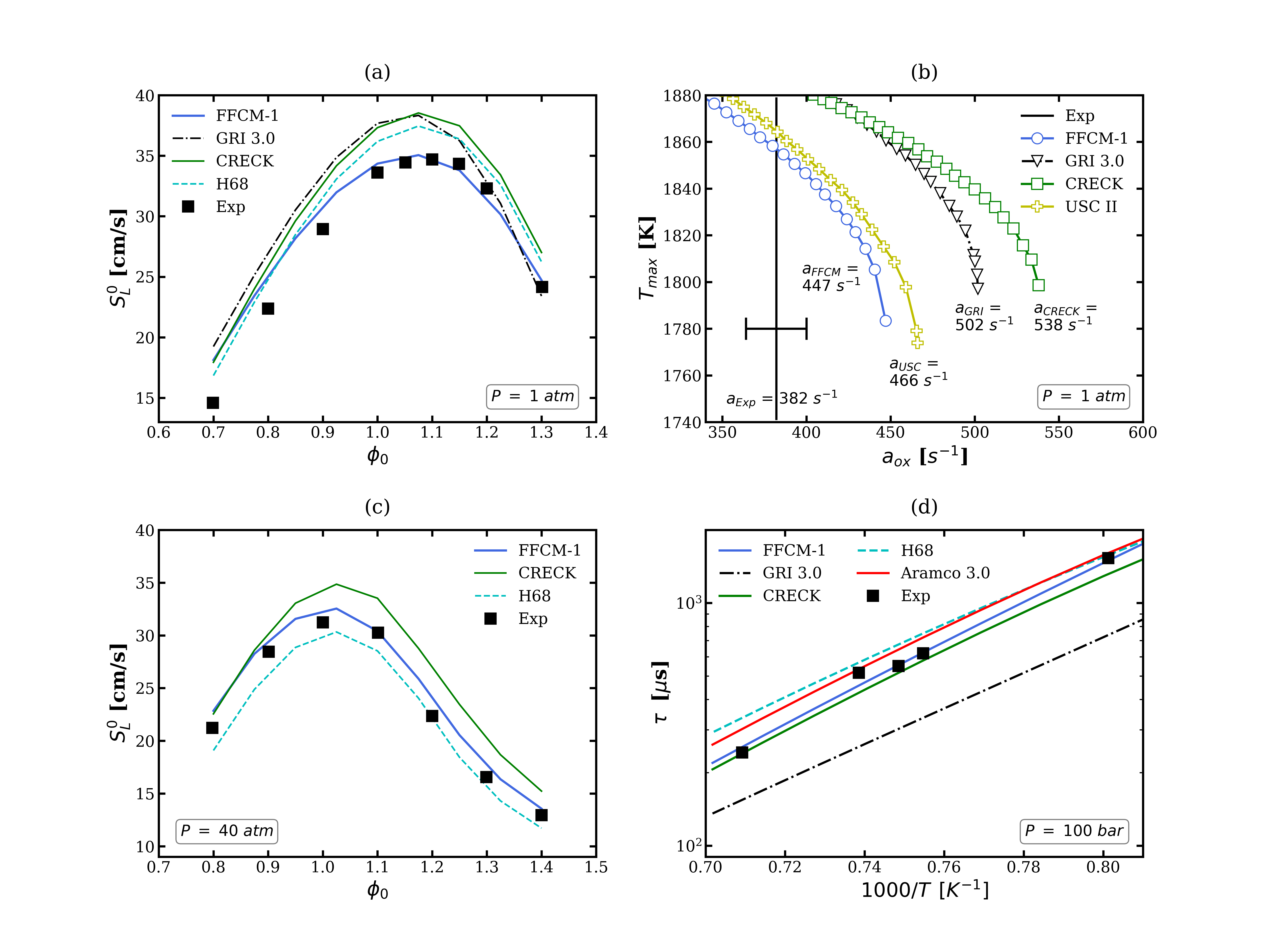
Figure 1: Validation of kinetic models against experimental data: (a) predictions of CH₄-air laminar flame speed vs. experimental data (square markers) of Lowry et al. [40] at $\phi_{0}=1.0$ and T₀ = 298 $K$, (b) predictions of CH₄-air diffusion flame extinction vs. experimental data of Chelliah et al. [42], which is shown as a vertical line with 95% confidence interval, (c) predictions of “CH₄/17% O₂/83% He” flame speed vs experimental data (square markers) of Rozenchan et al. [41] at $\phi_{0}$ = $1.0$ and T₀ = 300 $K$, (d) ignition delay predictions benchmarked against experimental data (square markers) of Karimi et al. [43] for a mixture of CH₄/O₂/Ar=3:6:91 (mole fraction).

2 F-OTD for Skeletal Reduction

2.1 Reduced-order modeling of the sensitivity with f-OTD

The temporal changes in mass fractions $\mbox{\boldmath$\psi$}=[\psi_{1},\psi_{2},\dots,\psi_{n_{s}}]^{T}$ of chemical species and temperature $T$ in an adiabatic, constant pressure $P$, and spatially homogeneous chemical system of $n_{s}$ species reacting through $n_{r}$ irreversible reactions are governed by the following initial value problem [44, 10]:

$$\frac{d\xi_{i}}{dt}=f_{i}\left(\mbox{\boldmath$\xi$},\mbox{\boldmath$\alpha$}\right),\ \ \mbox{\boldmath$\xi$}(0)=[\mbox{\boldmath$\psi$}_{0},T_{0}],$$ (1)

where $\mbox{\boldmath$\xi$}=[\mbox{\boldmath$\psi$},T]\in\mathbb{R}^{n_{eq}}$, $\mbox{\boldmath$f$}=[\mbox{\boldmath$f$}_{\mbox{\boldmath$\psi$}},f_{T}]$, $t$ is time, and $n_{eq}=n_{s}+1$. In Eq. (1), $\mbox{\boldmath$\alpha$}=[1,1,\dots,1]\in\mathbb{R}^{n_{r}}$ denotes the vector of sensitivity parameters perturbing the progress rate of reactions $\mathcal{Q}_{j}=\alpha_{j}\mathcal{k}_{j}\prod_{m=1}^{n_{s}}(\rho\psi_{m}/W_{m})^{\nu^{\prime}_{mj}}$ with $j=1,2,\dots,n_{r}$. Here, $\rho$ denotes the density, $\nu^{\prime}_{mj}$ is the molar stoichiometric coefficients of species $m$ in reaction $j$, and $W_{m}$ is the molecular weight of species $m$. A perturbation with respect to $\alpha_{j}$ around $\alpha_{j}=1$, implies an infinitesimal perturbation of $\mathcal{Q}_{j}$. The parameter $\mathcal{k}_{j}$ is the forward rate constant of reaction $j$, which is calculated via the modified Arrhenius model for elementary reactions [45]. All reversible reactions are cast as irreversible reactions. The matrix, $S(t)\in\mathbb{R}^{n_{eq}\times n_{r}}$, contains local sensitivity coefficients, $S_{ij}=\partial\xi_{i}/\partial\alpha_{j}$, and is evolved by solving the sensitivity equation:

$$\begin{split}\frac{dS_{ij}}{dt}&=\sum_{m=1}^{n_{eq}}\frac{\partial f_{i}}{\partial\xi_{m}}\frac{\partial\xi_{m}}{\partial\alpha_{j}}+\frac{\partial f_{i}}{\partial\alpha_{j}}=\sum_{m=1}^{n_{eq}}L_{im}S_{mj}+F_{ij},\end{split}$$ (2)

where $L_{im}=\frac{\partial f_{i}}{\partial\xi_{m}}$ and $F_{ij}=\frac{\partial f_{i}}{\partial\alpha_{j}}$ denote the Jacobian and the forcing matrices, respectively.

In f-OTD, the sensitivity matrix $S(t)$ is factorized into a time-dependent subspace in the $n_{eq}$-dimensional phase space of compositions represented by a set of f-OTD modes: $U(t)=[\mbox{\boldmath$u$}_{1}(t),\mbox{\boldmath$u$}_{2}(t),\dots,\mbox{\boldmath$u$}_{r}(t)]\in\mathbb{R}^{n_{eq}\times r}$. These modes are orthonormal: $\mbox{\boldmath$u$}_{i}^{T}(t)\mbox{\boldmath$u$}_{j}(t)=\delta_{ij}$, where $\delta_{ij}$ denotes the Kronecker delta function. The rank of $S(t)\in\mathbb{R}^{n_{eq}\times n_{r}}$ is $d=\mbox{min}\{n_{eq},n_{r}\}$, while the f-OTD modes represent a rank-$r$ subspace, where $r\ll d$. The sensitivity matrix is approximated via the f-OTD decomposition, $S(t)\approx U(t)Y^{T}(t)$, where $Y(t)=[\mbox{\boldmath$y$}_{1}(t),\mbox{\boldmath$y$}_{2}(t),\dots,\mbox{\boldmath$y$}_{r}(t)]\in\mathbb{R}^{n_{r}\times r}$ is the f-OTD coefficient matrix. Therefore, each sensitivity coefficient $S_{ij}$ can be approximated as a finite sum of time-dependent terms: $S_{ij}(t)\approx\sum_{k=1}^{r}U_{ik}(t)Y_{jk}(t)$. The key characteristic of the model is that both $U(t)$ and $Y(t)$ are time-dependent, and evolve according to the closed form evolution equations extracted from the governing equations of the system [10]:

$$\frac{dU}{dt} = QLU+QFYC^{-1},$$ (3a)

$$\frac{dY}{dt} = YL_{r}^{T}+F^{T}U,$$ (3b)

where $L_{r}=U^{T}LU\in\mathbb{R}^{r\times r}$ is a reduced linearized operator, $Q=I-UU^{T}$ is the orthogonal projection onto the space spanned by the complement of $U$, and $C=Y^{T}Y\in\mathbb{R}^{r\times r}$ is a correlation matrix. The model constructed in this way is able to capture sudden transitions associated with the largest finite time Lyapunov exponents [46, 47]. Equation (3) is a coupled system of ODEs and constitutes the f-OTD evolution equations. The matrix $C(t)$ is, generally full, implying that the f-OTD coefficients are correlated. The f-OTD modes can become uncorrelated and energetically ranked by rotating the modes along the eigen-direction of the matrix $C$. When the energy of some of the f-OTD modes are dominant and their singular values are orders of magnitude larger than the energy associated with the other modes, it would be better to use the rank-adaptive and sparse-sampling f-OTD methodology [48, 49]. This would circumvent numerical instabilities due to the presence of $C^{-1}$ in Eq. (3a). The f-OTD modes align themselves with the most instantaneously sensitive directions of the composition evolution equation when perturbed by $\alpha$. These directions can be unambiguously defined as the rank-$r$ reduction of instantaneous singular value decomposition (SVD) of $S(t)$. It has been shown that f-OTD closely approximates the instantaneous SVD of $S(t)$, and also approximates sensitive directions without having access to any data on full-dimensional $S(t)$ [10]. Similar methodologies via time-dependent bases have also been utilized in stochastic ROM [50, 51, 52, 53, 29], flow control [54], rare events predictions [55], and ROM of transport equations [56, 57].

2.2 Important reactions & species

In f-OTD, modeled sensitivities are computed in factorized format by solving Eqs. (3), in addition to Eq. (1), and the values of $\xi$, $U$, and $Y$ are stored at resolved time steps $t_{i}\in[0,t_{f}]$. At each resolved time step, and for each case, the eigen decomposition of $S^{T}S\in\mathbb{R}^{n_{r}\times n_{r}}$ as $S^{T}S=A\Lambda A^{T}$ are computed along with $\mbox{\boldmath$w$}\in\mathbb{R}^{n_{r}\times 1}=(\Sigma\lambda_{i}|\mbox{\boldmath$a$}_{i}|)/(\Sigma\lambda_{i})\in\mathbb{R}^{n_{r}}$. The $w$ vectors are basically the average of eigenvectors of $S^{T}S$ matrix weighted based on their associated eigenvalues. This prevents the f-OTD method from dealing with each eigenvector ($\mbox{\boldmath$a$}_{i}$) separately. The first sorted eigenvalue ($\lambda_{1}$) is usually orders of magnitude larger than the others, which implies $\mbox{\boldmath$w$}(t)\approx|\mbox{\boldmath$a$}_{1}(t)|$. Each element of $w$, i.e. $w_{i}$, is positive and associated with a certain reaction ($i$th reaction). The larger the $w_{i}$ value, the more important the reaction $i$ is. The variable $\chi_{i}$ is used to define as the highest value associated with $w_{i}$, i.e. $\chi_{i}=max_{t}(w_{i}(t))$.

The elements of $\chi$ vector are sorted in descending order to find the indices of the most important reactions in the detailed model. Species are also sorted based on their first presence in the sorted reactions, i.e. the species which first shows up in a higher ranked reaction are more important than a species that first participate in a lower ranked reaction. This yields in a reaction and species ranking based on the $\chi$ vector. Finally, a set of species are chosen by setting the threshold $\chi_{\epsilon}$ on the element of $\chi$ vector and eliminating species whose associated $\chi_{i}$ values are smaller. The skeletal model reduction is reaction based, thus any non-reactive species with non-zero mass fraction in the initial condition should be manually added to the skeletal model, such as N₂ and/or Ar.

In summary, the f-OTD method instantaneously observes the ignition system, and sorts the reactions based on their effects on sensitivities to find the most important species. These species and the reactions which connect them together create the skeletal models. In chemical kinetic systems, perturbations with respect to “fast” reactions generate very large sensitivities for short time periods, but these sensitivities vanish as $t\rightarrow\infty$. On the other hand, perturbations with respect to “slow” reactions generate smaller and more sustained sensitivities. Since the approach is based on the instantaneous observation of sensitivities, both slow and fast reactions can leave an imprint on the instantaneous normalized reaction vector ($w$). However, if the sensitivities associated with these reactions would be averaged together over a period of time, then the smaller sensitivities associated with slow reactions could be out-weighted by the large sensitivities associated with fast reactions.

3 Skeletal Reduction of FFCM-1

The f-OTD method is employed to compute local sensitivities based on Eq. (3) for atmospheric and high pressure ignition of methane. The $U$ and $Y$ matrices are initialized by solving the sensitivity equation (Eq. (2)) for few time steps, and then performing singular value decomposition on the sensitivity matrix. All f-OTD simulations are performed with $r=2$. The initial conditions for temperature, pressure, and equivalence ratio are $T_{0}\in\{1200,1500,2000\}$ $K$, $P\in\{1,20,40,60,80,100\}$ $atm$, and $\phi\in\{0.5,1.0,1.5\}$, respectively. Therefore, in total 48 cases are considered. As described in §2, the outcome of the reduction process is a series of skeletal models as listed in Table 1. The generated f-OTD models are labeled by “f-OTD-X” in which “X” denotes the number of species included in the model. In Table 1, $n_{r}$ shows the number of irreversible reactions in each of the models.

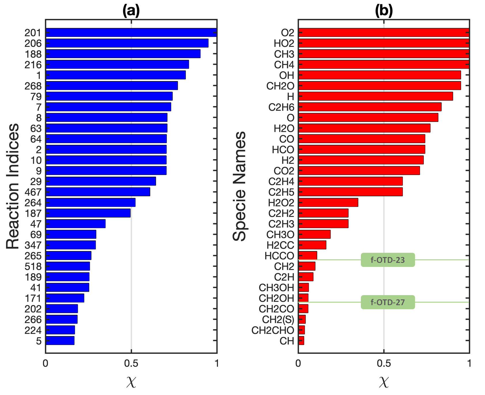
Figure 2: The FFCM-1 skeletal reduction for methane-air: sorted (a) reactions and (b) species based on their importance as determined by their associated $\chi$ values.

Table 1: FFCM-1 based skeletal models

Model	$n_{s}$	$n_{r}$	$\chi_{\epsilon}$
FFCM-1	38	569	0
f-OTD-27	27	319	0.0583
f-OTD-25	25	261	0.0877
f-OTD-24	24	247	0.0992
f-OTD-23	23	213	0.1093

3.1 Reactions and species ranking

Figure 2 shows the species and reaction rankings based on the process described in §2.2. Reactions R201 (O₂ + CH₄ $\rightarrow$ CH₃ + HO₂), R206 ( CH₃ + O₂ $\rightarrow$ OH + CH₂O), and R188 (CH₄ (+M) $\rightarrow$ CH₃ + H (+M)) are identified as the top three most important ones in FFCM-1 for methane ignition. The oxidation of methane is initiated by its reaction with molecular oxygen (R201). The methyl radical (CH₃) then reacts with the molecular oxygen to form OH + CH₂O via R206. As for the species, O₂, HO₂, CH₃, CH₄, OH, CH₂O, H, C₂H₆, O, H₂O are the top 10 most important ones. The f-OTD-23 model contains the top 22 ranked species in Fig. 2(b) plus nitrogen (non-reactive species with non-zero initial mass fractions). The f-OTD-24, f-OTD-25, f-OTD-26, and f-OTD-27 models are produced by adding, respectively, CH₂, C₂H, CH₃OH, and CH₂OH and their reactions step by step to f-OTD-23.

3.2 Skeletal model validation

The performances of the reduced models are assessed by comparing their estimations for the ignition delays, the laminar flame speeds, and the counter-flow extinction strains against FFCM-1 for different mixtures. Here, the ignition delay is defined as the time required by carbon monoxide (CO) to reach its maximum production rate. The flame speeds and the extinction curves are generated by Cantera [58] with a plug flow boundary condition assumption [59] for extinction simulations.

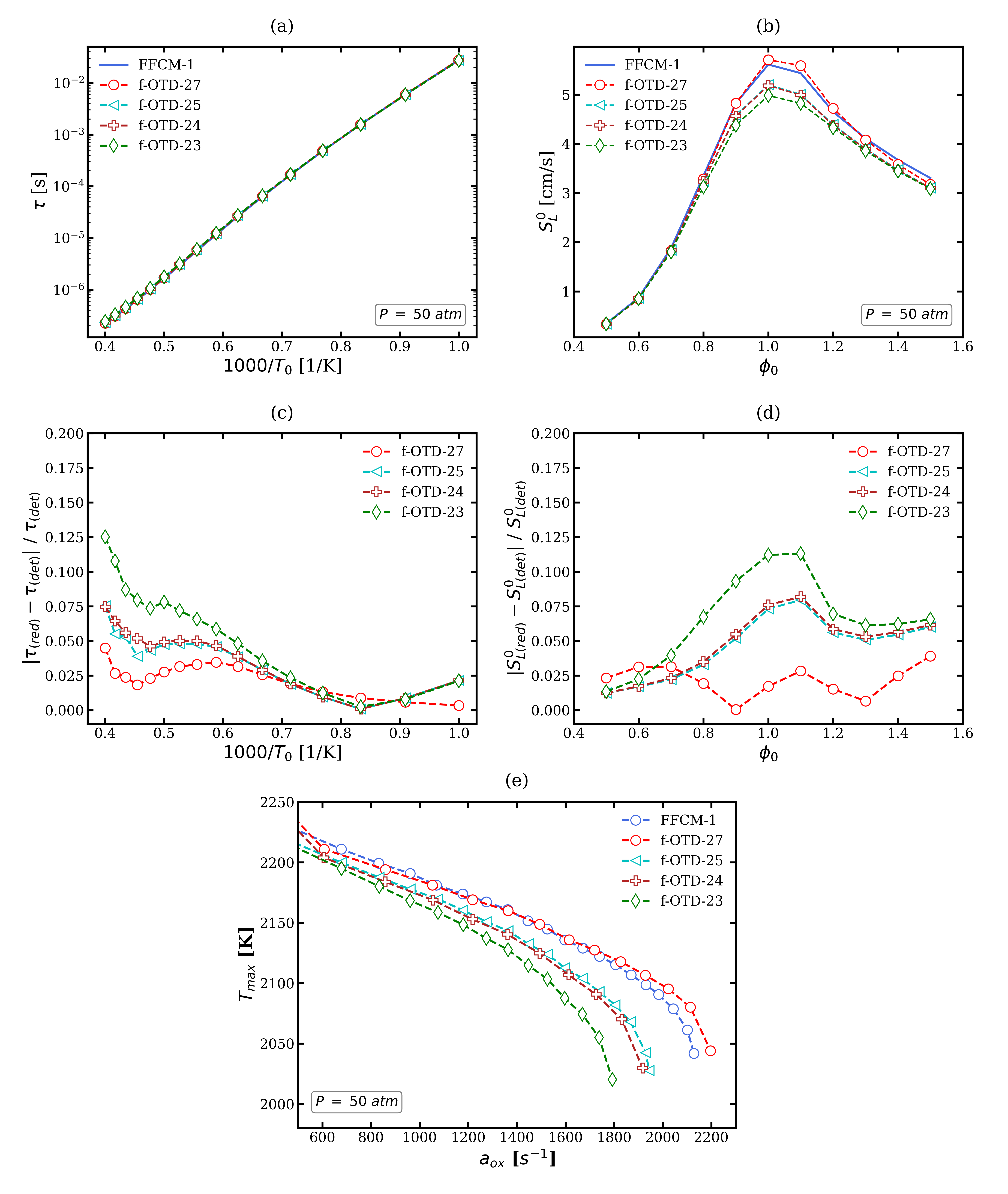
Figure 3: Predictions via f-OTD skeletal models at $P=50$ $atm$: (a) ignition delays, $\phi_{0}=1.0$, (b) flame speeds, $T_{0}=300$ $K$, (c) relative errors of skeletal models in terms of the ignition delays, (d) relative errors of skeletal models in terms of the flame speeds, (e) nonpremixed flame extinction with $T_{0}=300$ $K$.

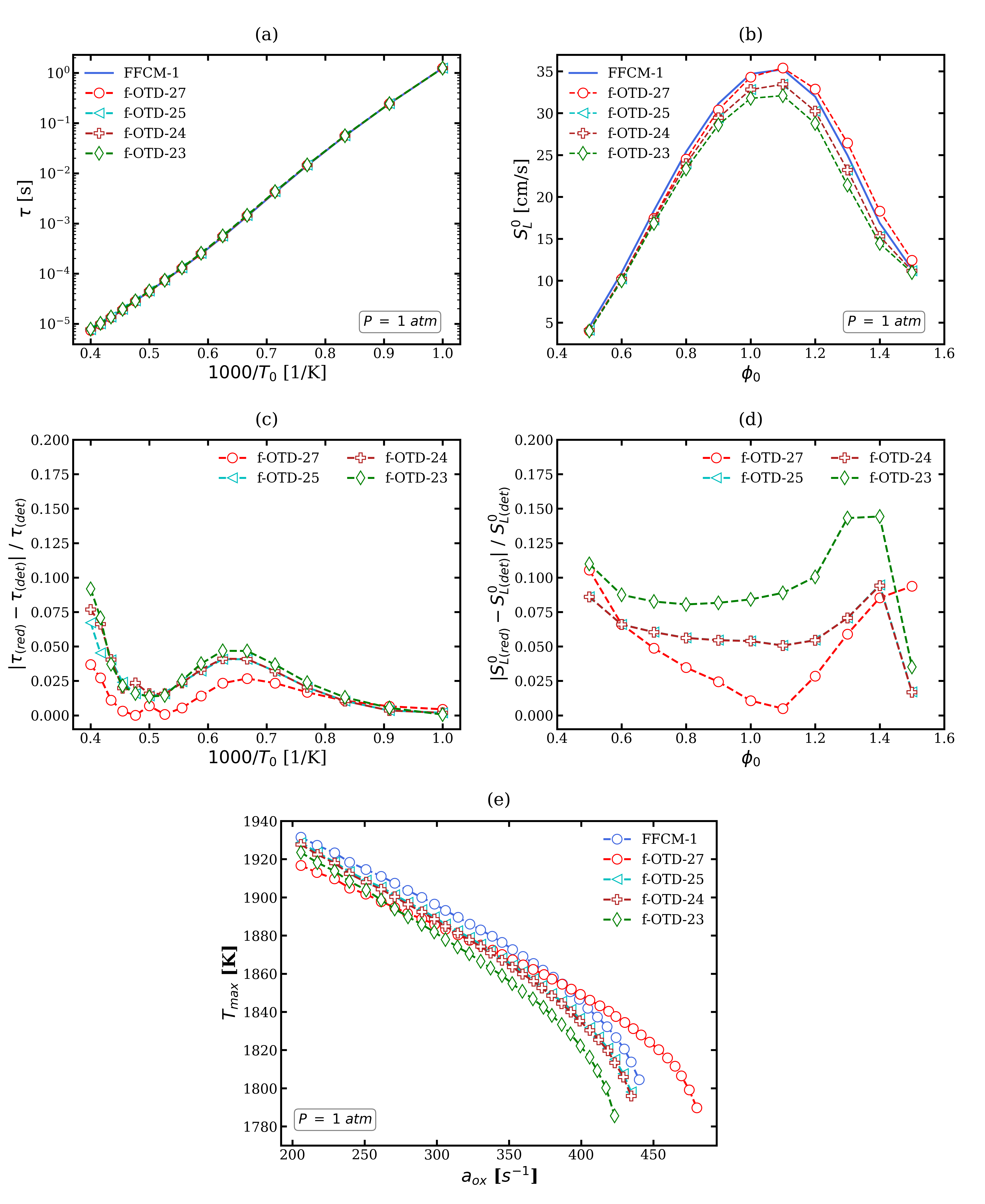
Figure 4: Predictions via f-OTD skeletal models at $P=1$ $atm$: (a) the ignition delays, $\phi_{0}=1.0$, (b) the flame speeds, $T_{0}=300$ $K$, (c) relative errors of skeletal models in terms of ignition delays, (d) relative errors of skeletal models in terms of the flame speeds, (e) nonpremixed flame extinction, $T_{0}=300$ $K$.

Figure 3 compares the f-OTD results at $P=50$ $atm$ against FFCM-1. Figure 3(a) and (c) show that f-OTD models with $n_{s}\geq 24$ predict ignition delays with less than 10% error for $T_{0}\in[1000,2500]K$, and less than 5% error for $T_{0}\in[1000,1670]K$. The f-OTD-27 is the most accurate skeletal model for estimating ignition delays at $P=50$ $atm$ with less than 5% overall error. Figure 3(b) and (d) portray the ability of f-OTD-24, f-OTD-25, and f-OTD-27 models in reproducing the laminar flame speeds of FFCM-1 with less than 10% error. The maximum error of f-OTD-27 for flame speed estimations is 3%. Figure 3(e) shows that the f-OTD model with 27 species reproduces the extinction curve of FFCM-1 almost exactly. Altogether, the accuracy of f-OTD models in regenerating FFCM-1 results improves with increasing the number of species. Moreover, f-OTD-24 and f-OTD-25 show very similar predictions. This means that while C₂H is an important species, including it in f-OTD-25 does not change the predictions significantly.

Figure 4 shows the performance of f-OTD models at $P=1$ $atm$. Figures 4(a), (b), (c), and (d) indicate better performances of the models in predicting the ignition delays and the laminar flame speeds by increasing $n_{s}$. The f-OTD-27 is the most accurate model with less than 5% error in estimating ignition delays, and 10% error in predicting laminar flame speeds. However, the flame speeds calculated by f-OTD-27 have larger errors for very lean and very rich fuels, i.e. $\phi_{0}<0.6$ and $\phi_{0}>1.4$. Altogether, Fig. 4 suggests that at atmospheric pressure, f-OTD model with $n_{s}\geq 24$ provides reasonable predictions for the three quantities as considered.

Figures 5 - 7 demonstrate the ability of f-OTD-24 and f-OTD-27 in reproducing the FFCM-1 results, over a wide range of pressures ($P=60$ $atm$, $80$ $atm$, and $100$ $atm$). Figure 5 compares the ignition delays predicted by these f-OTD models against FFCM-1, and Fig. 6 indicates that f-OTD-24 and f-OTD-27 estimate the FFCM-1 flame speeds accurately. The f-OTD-27 predicts the laminar flame speeds reasonably well, with its worst predictions at $\phi_{0}>$1.2 where the relative error is still less than 10%. Figure 6 also shows that the maximum flame speed decreases by increasing the pressure from $60$ $atm$ to $100$ $atm$. Figure 7 compares the extinction curves of f-OTD-24 and f-OTD-27 against FFCM-1. Both models perform very well in this high pressure condition. Figure 8 shows the structure of freely-propagating, premixed flame of methane at two different pressures, i.e. $P=1$ $atm$ and $P=50$ $atm$. f-OTD-24 and f-OTD-27 reproduce the temperature and mass fractions predictions of FFCM-1 with a good accuracy.

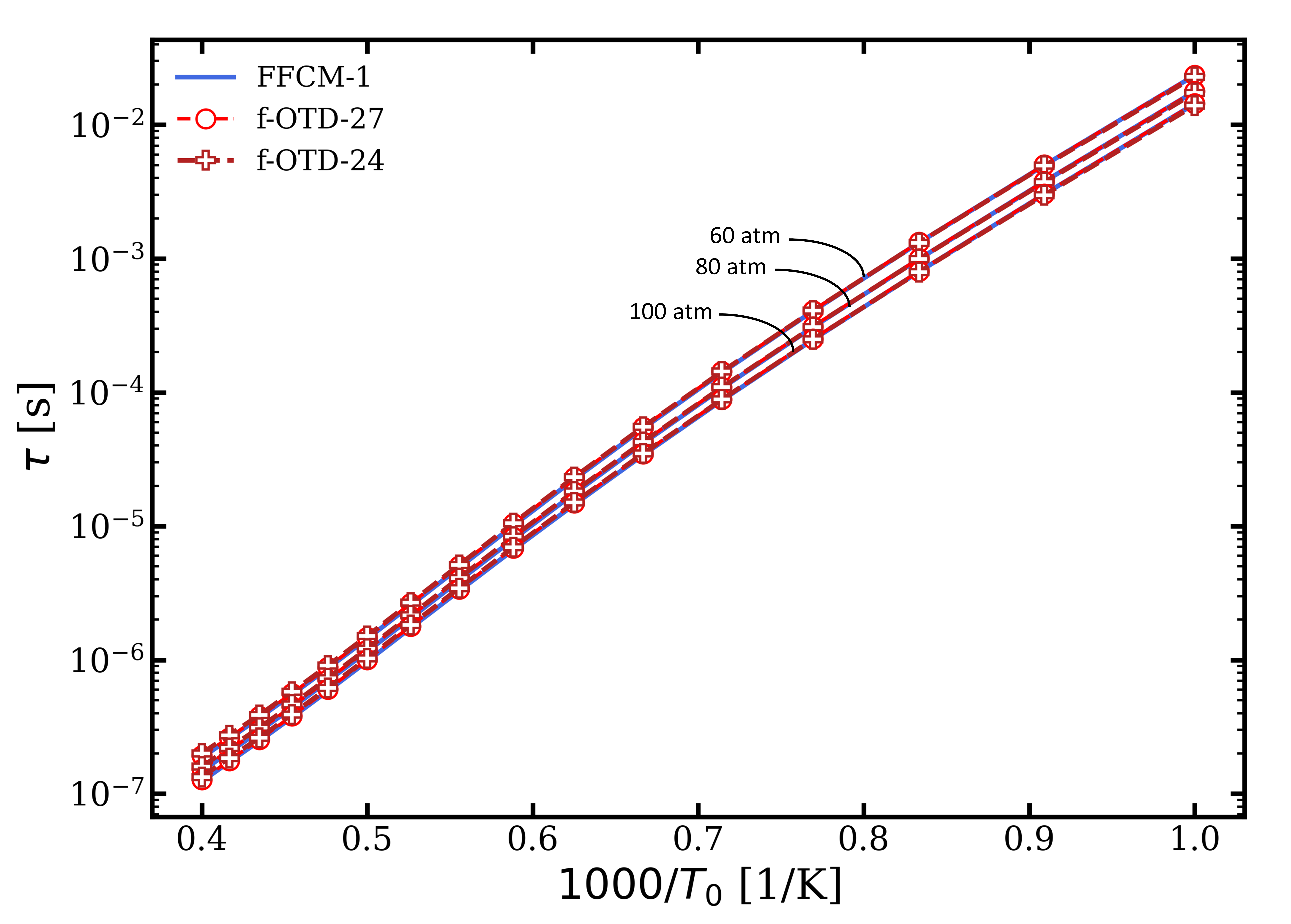
Figure 5: Predictions via f-OTD-24 and f-OTD-27: Ignition delays for $P=60,80$, and $100$ $atm$ with $\phi_{0}=1.0$.

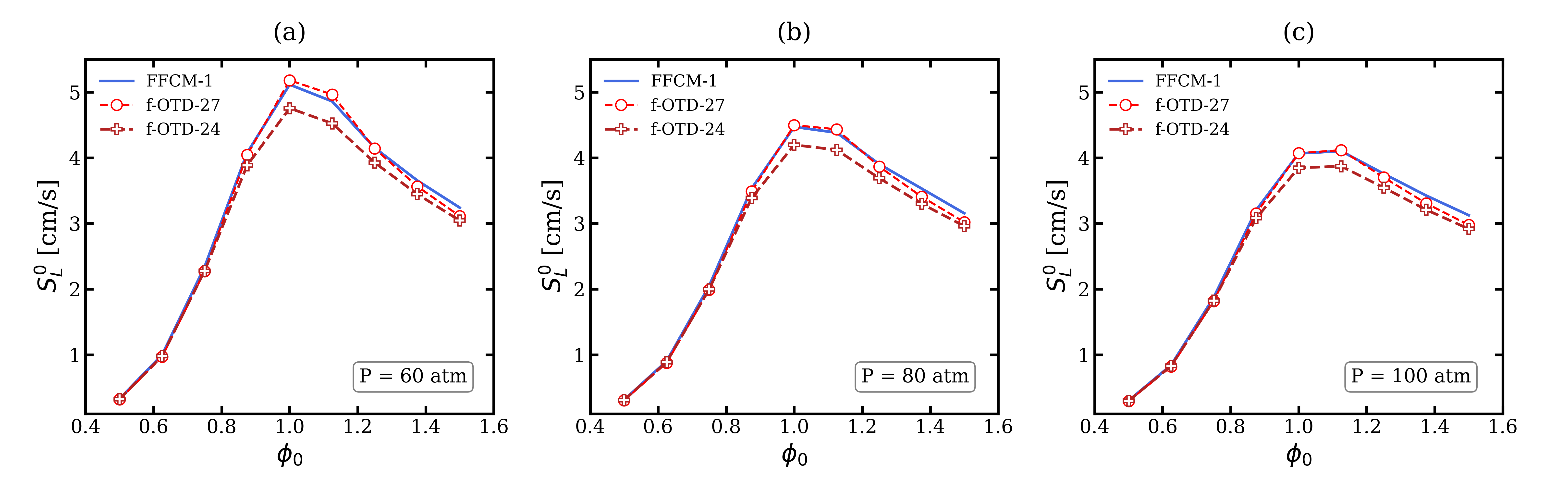
Figure 6: Predictions via f-OTD-24 and f-OTD-27: Laminar flame speeds for $P=60,80$, and $100$ $atm$ with $T_{0}=300$ $K$.

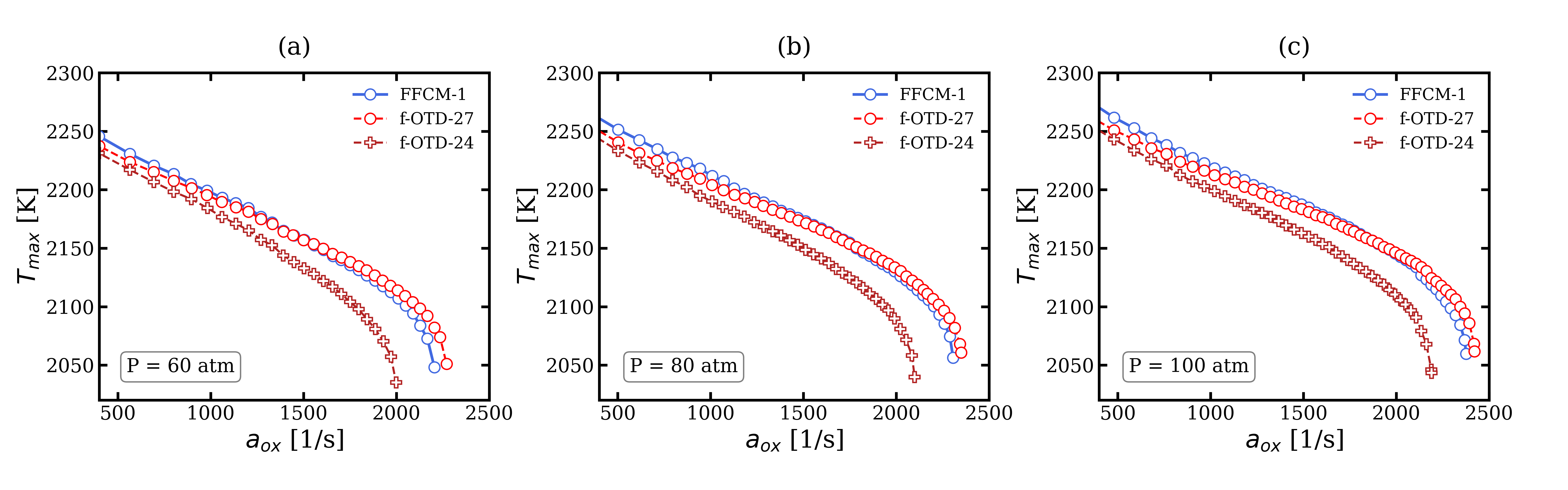
Figure 7: Predictions via f-OTD-24 and f-OTD-27: Diffusion flame extinction for $P=60,80$, and $100$ $atm$ with $T_{0}=300$ $K$.

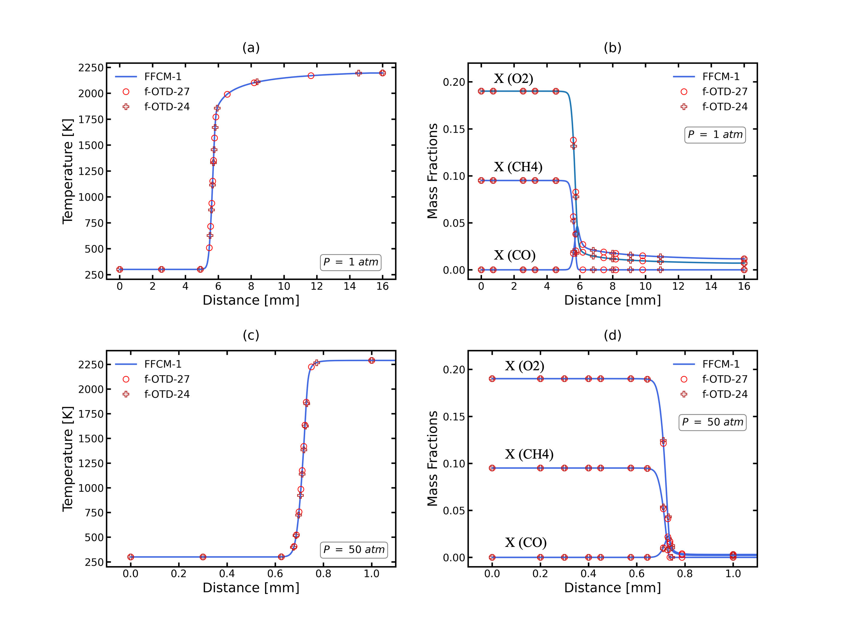
Figure 8: Prediction via f-OTD-24 and f-OTD-27: 1 D freely-propagating, premixed flame structure with $T_{0}$ $=$ $300$ $K$, $\phi_{0}$ $=$ $1.0$, and $P=1\&50$ $atm$

4 Conclusions

New skeletal kinetics models are generated from the FFCM-1 for the methane combustion at atmospheric and high pressure conditions. In the reduction process, local sensitivities are computed by the f-OTD method for the auto-ignition problem with different sets of initial conditions. The calculated sensitivities are then analyzed, and the 38 species of the FFCM-1 are ranked based on their importance. Different skeletal models with different levels of accuracy are generated by selecting more high ranked species. The ignition delays, the laminar flame speeds, and the diffusion flame extinctions predicted by the generated models are benchmarked against FFCM-1. The results show the model with 27 species and 319 irreversible reactions accurately reproduces the predictions of FFCM-1 at all conditions. The model with 24 species and 247 irreversible reactions also provides reasonable predictions. Therefore, f-OTD-24 and f-OTD-27 are the recommended skeletal models for the FFCM-1 over the observed range of pressures, temperatures, and equivalence ratios. The Cantera format (.cti) of these skeletal models are supplied in the Appendix.

The f-OTD method has demonstrated its ability for reduced order modeling of local sensitivities in time dependent combustion systems, and is recommended for future multi-dimensional reacting flow simulations. The described local sensitivity analysis technique for skeletal reduction is also recommended for other detailed kinetics models. This technique does not require a priori expert knowledge of chemistry, thus can be used for skeletal reduction of very large reaction networks, e.g. heavy hydrocarbon fuels like JP-10 (C₁₀H₁₆). For future work the f-OTD method is recommended for skeletal reduction of very large reaction networks, i.e. with $\mathcal{O}(1000)$ species, by implementing rank-adaptive and sparse-sampling techniques  [48, 49].

Appendix

All reduced mechanisms developed in this work can be accessed via this link.

References

- [1] K. Kohse Höinghaus, Combustion in The Future: The Importance of Chemistry, Proc. Combust. Inst. 38 (1) (2021) 1–56.
- [2] A.N.Gorban, Model Reduction in Chemical Dynamics: Slow Invariant Manifolds, Singular Perturbations, Thermodynamic Estimates, and Analysis of Reaction Graph, Curr. Opin. Chem. Eng. 21 (2018) 48–59.
- [3] T. Lu, C. Law, Toward Accommodating Realistic Fuel Chemistry in Large-Scale Computations, Prog. Energy Combust. Sci. 35 (2) (2009) 192–215.
- [4] D. Goussis, U. Maas, Model Reduction for Combustion Chemistry, in: Turbulent combustion modeling, Springer, 2011, pp. 193–220.
- [5] M. D. Smooke, Reduced Kinetic Mechanisms and Asymptotic Approximations for Methane-Air Flames: A Topical Volume, Springer, 1991.
- [6] N. Peters, B. Rogg (Eds.), Reduced Kinetic Mechanisms for Applications in Combustion Systems, Vol. 15 of Lecture Notes in Physics, Springer-Verlag, Berlin, Germany, 1993.
- [7] T. Turányi, Sensitivity Analysis of Complex Kinetic Systems. Tools and Applications, J. Math. Chem. 5 (3) (1990) 203–248.
- [8] A. S. Tomlin, The Role of Sensitivity and Uncertainty Analysis in Combustion Modelling, Proc Combust Inst 34 (1) (2013) 159–176.
- [9] F. vom Lehn, L. Cai, H. Pitsch, Sensitivity Analysis, Uncertainty Quantification, and Optimization for Thermochemical Properties in Chemical Kinetic Combustion Models, Proc Combust Inst 37 (1) (2019) 771–779.
- [10] A. Nouri, H. Babaee, P. Givi, H. Chelliah, D. Livescu, Skeletal Model Reduction with Forced Optimally Time Dependent Modes, Combust. Flame 235 (2022) 111684.
- [11] S. Lam, D. Goussis, The CSP Method for Simplifying Kinetics, Int. J. Chem. Kinet. 26 (4) (1994) 461–486.
- [12] M. Neophytou, D. Goussis, M. Van Loon, E. Mastorakos, Reduced Chemical Mechanisms for Atmospheric Pollution Using Computational Singular Perturbation Analysis, Atmos. Environ. 38 (22) (2004) 3661–3673.
- [13] T. Lu, C. K. Law, A Criterion Based on Computational Singular Perturbation for The Identification of Quasi Steady State Species: A Reduced Mechanism for Methane Oxidation with No Chemistry, Combust. Flame 154 (4) (2008) 761–774.
- [14] T. Turanyi, Reduction of Large Reaction Mechanisms, New J. Chem. 14 (11) (1990) 795–803.
- [15] H. Wang, M. Frenklach, Detailed Reduction of Reaction Mechanisms for Flame Modeling, Combust. Flame 87 (3-4) (1991) 365–370.
- [16] W. Sun, Z. Chen, X. Gou, Y. Ju, A Path Flux Analysis Method for The Reduction of Detailed Chemical Kinetic Mechanisms, Combust. Flame 157 (7) (2010) 1298–1307.
- [17] T. Lu, C. K. Law, A Directed Relation Graph Method for Mechanism Reduction, Proc. Combust. Inst. 30 (1) (2005) 1333–1341.
- [18] P. Pepiot-Desjardins, H. Pitsch, An Efficient Error-propagation-based Reduction Method for Large Chemical Kinetic Mechanisms, Combust. Flame 154 (1-2) (2008) 67–81.
- [19] K. E. Niemeyer, C.-J. Sung, M. P. Raju, Skeletal Mechanism Generation for Surrogate Fuels Using Directed Relation Graph with Error Propagation and Sensitivity Analysis, Combust. Flame 157 (9) (2010) 1760–1770.
- [20] N. Brown, G. Li, M. Koszykowski, Mechanism Reduction via Principal Component Analysis, Int. J. Chem. Kinet. 29 (6) (1997) 393–414.
- [21] G. Esposito, H. Chelliah, Skeletal Reaction Models Based on Principal Component Analysis: Application to Ethylene–Air Ignition, Propagation, and Extinction Phenomena, Combust. Flame 158 (3) (2011) 477–489.
- [22] A. Parente, J. Sutherland, B. Dally, L. Tognotti, P. Smith, Investigation of The MILD Combustion Regime via Principal Component Analysis, Proc. Combust. Inst. 33 (2) (2011) 3333–3341.
- [23] A. Parente, J. Sutherland, Principal Component Analysis of Turbulent Combustion Data: Data Pre-processing and Manifold Sensitivity, Combust. Flame 160 (2) (2013) 340–350.
- [24] H. Mirgolbabaei, T. Echekki, Nonlinear Reduction of Combustion Composition Space with Kernel Principal Component Analysis, Combust. Flame 161 (1) (2014) 118–126.
- [25] A. Coussement, B. Isaac, O. Gicquel, A. Parente, Assessment of Different Chemistry Reduction Methods based on Principal Component Analysis: Comparison of The MG-PCA and Score-PCA Approaches, Combust. Flame 168 (2016) 83–97.
- [26] M. Malik, B. Isaac, A. Coussement, P. Smith, A. Parente, Principal Component Analysis Coupled with Nonlinear Regression for Chemistry Reduction, Combust. Flame 187 (2018) 30–41.
- [27] A. Stagni, A. Frassoldati, A. Cuoci, T. Faravelli, E. Ranzi, Skeletal Mechanism Reduction Through Species-Targeted Sensitivity Analysis, Combust. Flame 163 (2016) 382–393.
- [28] M. Donello, M. H. Carpenter, H. Babaee, Computing Sensitivities in Evolutionary Systems: A Real-Time Reduced Order Modeling Strategy, SIAM J. Sci. Comput. (2022) A128–A149.
- [29] P. Patil, H. Babaee, Real-Time Reduced-Order Modeling of Stochastic Partial Differential Equations Via Time-Dependent Subspaces, J. Comput. Phys. 415 (2020) 109511.
- [30] O. Koch, C. Lubich, Dynamical Low-Rank Approximation, SIAM J. Matrix Anal. Appl 29 ( 2) ( 2007) 434–454.
- [31] G. P. Smith, D. M. Golden, M. Frenklach, N. W. Moriarty, B. Eiteneer, M. Goldenberg, C. T. Bowman, R. K. Hanson, S. Song, W. C. Gardiner Jr., V. V. Lissianski, Z. Qin, Gri-Mech 3.0, http://www.me.berkeley.edu/gri_mech/.
-
[32]
H. Wang, X. You, A. V. Joshi, S. G. Davis, A. Laskin, F. Egolfopoulos, C. K.
Law, Usc Mech Version
ii. High-temperature Combustion Reaction Model of h2/co/c1-c4
Compounds.
URL http://ignis.usc.edu/USC_Mech_II.htm - [33] E. Ranzi, A. Frassoldati, R. Grana, A. Cuoci, T. Faravelli, A. Kelley, C. Law, Hierarchical and Comparative Kinetic Modeling of Laminar Flame Speeds of Hydrocarbon and Oxygenated Fuels, Prog. Energy Combust. Sci. 38 (4) (2012) 468–501.
- [34] G. Smith, Y. Tao, H. Wang, Foundational Fuel Chemistry Model Version 1.0 (ffcm-1), 2016, URL: http://nanoenergy. stanford. edu/ffcm1.
- [35] C. W. Zhou, Y. Li, U. Burke, C. Banyon, K. P. Somers, S. Ding, S. Khan, J. W. Hargis, T. Sikes, O. Mathieu, et al., An Experimental and Chemical Kinetic Modeling Study of 1, 3-butadiene Combustion: Ignition Delay Time and Laminar Flame Speed Measurements, Combust. Flame 197 (2018) 423–438.
- [36] H. Hashemi, J. M. Christensen, S. Gersen, H. Levinsky, S. J. Klippenstein, P. Glarborg, High-Pressure Oxidation of Methane, Combust. Flame 172 (2016) 349–364.
- [37] M. Pierro, A. Laich, J. J. Urso, C. Kinney, S. Vasu, M. A. Albright, Ignition Delay Times of Methane Fuels at Thrust Chamber Conditions in An Ultra-high-pressure Shock Tube, in: AIAA SCITECH 2022 Forum, 2022, p. 1254.
- [38] J. Shao, A. M. Ferris, R. Choudhary, S. J. Cassady, D. F. Davidson, R. K. Hanson, Shock-induced Ignition and Pyrolysis of High-pressure Methane and Natural Gas Mixtures, Combust. Flame 221 (2020) 364–370.
- [39] Y. Li, C. W. Zhou, K. P. Somers, K. Zhang, H. J. Curran, The Oxidation of 2-Butene: A High Pressure Ignition Delay, Kinetic Modeling Study and Reactivity Comparison With Isobutene and 1-Butene, Proc. Combust. Inst. 36 (1) (2017) 403–411.
- [40] W. Lowry, J. de Vries, M. Krejci, E. Petersen, Z. Serinyel, W. Metcalfe, H. Curran, G. Bourque, Laminar Flame Speed Measurements and Modeling of Pure Alkanes and Alkane Blends at Elevated Pressures, J Eng Gas Turbine Power 133 (9).
- [41] G. Rozenchan, D. L. Zhu, C. K. Law, S. D. Tse, Outward Propagation, Burning Velocities, and Chemical Effects of Methane Flames Up to 60 Atm, Proc Combust Inst 29 (2) (2002) 1461–1470.
- [42] B. Sarnacki, G. Esposito, R. Krauss, H. Chelliah, Extinction Limits and Associated Uncertainties of Nonpremixed Counterflow Flames of Methane, Ethylene, Propylene and n-Butane in Air, Combust. Flame 159 (3) (2012) 1026–1043.
- [43] M. Karimi, B. Ochs, Z. Liu, D. Ranjan, W. Sun, Measurement of Methane Autoignition Delays in Carbon Dioxide and Argon Diluents at High Pressure Conditions, Combust. Flame 204 (2019) 304–319.
- [44] I. Zsely, J. Zador, T. Turanyi, Similarity of Sensitivity Functions of Reaction Kinetic Models, J. Phys. Chem. A 107 (13) (2003) 2216–2238.
- [45] F. A. Williams, Combustion Theory, 2nd Ed., CRC Press, Taylor Francis Group, London, 1985.
- [46] H. Babaee, T. Sapsis, A Minimization Principle for The Description of Modes Associated with Finite-Time Instabilities, Proc. R. Soc. A 472 (2186) (2016) 20150779.
- [47] H. Babaee, M. Farazmand, G. Haller, T. Sapsis, Reduced-Order Description of Transient Instabilities and Computation of Finite-time Lyapunov Exponents, Chaos 27 (6) (2017) 063103.
- [48] M. Donello, G. Palkar, M. H. Naderi, D. C. Del Rey Fernández, H. Babaee, CUR Decomposition for Scalable Rank-Adaptive Reduced-Order Modeling of Nonlinear Stochastic PDEs with Time-Dependent Bases, arXiv:2305.04291 (2023).
- [49] M.H. Naderi, H. Babaee, Adaptive Sparse Interpolation for Accelerating Nonlinear Stochastic Reduced-order Modeling with Time-Dependent Bases, Comput Methods Appl Mech Eng 405 ( 2023) 115813.
- [50] T. Sapsis, P. Lermusiaux, Dynamically Orthogonal Field Equations for Continuous Stochastic Dynamical Systems, Physica D: Nonlinear Phenom. 238 (23-24) (2009) 2347–2360.
- [51] M. Cheng, T. Hou, Z. Zhang, A Dynamically Bi-Orthogonal Method for Time-Dependent Stochastic Partial Differential Equations i: Derivation and Algorithms, J. Comput. Phys. 242 (2013) 843–868.
- [52] H. Babaee, M. Choi, T. P. Sapsis, G. E. Karniadaki, A Robust Bi-Orthogonal/Dynamically-Orthogonal Method Using The Covariance Pseudo-Inverse with Application to Stochastic Flow Problems, J. Comput. Phys. 344 (2017) 303–319.
- [53] H. Babaee, An Observation-Driven Time-Dependent Basis for A Reduced Description of Transient Stochastic Systems, Proc. R. Soc. A: Math. Phys. Eng. Sci. 475 (2231) (2019) 20190506.
- [54] A. Blanchard, S. Mowlavi, T. Sapsis, Control of Linear Instabilities by Dynamically Consistent Order Reduction on Optimally Time-dependent Modes, Nonlinear Dyn. 95 (4) (2019) 2745–2764.
- [55] M. Farazmand, T. Sapsis, Dynamical Indicators for The Prediction of Bursting Phenomena in High-dimensional Systems, Phys. Rev. E 94 (2016) 032212.
- [56] D. Ramezanian, A. Nouri, H. Babaee, On-The-Fly Reduced Order Modeling of Passive and Reactive Species via Time-dependent Manifolds, Comput. Methods Appl. Mech. Eng. 382 (2021) 113882.
- [57] A. Amiri-Margavi, H. Babaee, On-The-Fly Reduced-Order Modeling of Transient Flow Response Subject to High-Dimensional External Forcing, American Physical Society Division of Fluid Dynamics, Indianapolis, IN, Nov 2022. .
- [58] D. Goodwin, H. Moffat, R. Speth, Cantera: An Object-oriented Software Toolkit for Chemical Kinetics, Thermodynamics, and Transport Processes, http://www.cantera.org, Version 2.6.0 (2017).
- [59] T. Fiala, T. Sattelmayer, Nonpremixed Counterflow Flames: Scaling Rules for Batch Simulations, J. Combust. 2014.