Modified Brans-Dicke cosmology with Minimum Length Uncertainty

Abstract

We consider a modification of the Brans-Dicke gravitational Action Integral inspired by the existence of a minimum length uncertainty for the scalar field. In particular the kinetic part of the Brans-Dicke scalar field is modified such that the equation of motion for the scalar field be modified according  to the quadratic Generalized Uncertainty Principle (GUP). For the background geometry we assume the homogeneous and isotropic Friedmann–Lemaître–Robertson–Walker metric. We investigate the dynamics and the cosmological evolution for the dynamical variables of the theory and we compare the results with the unmodified Brans-Dicke theory. It follows that in consideration because of the additional degrees of freedom in the energy-momentum tensor the dynamical variables describe various aspects of the cosmological history. This is one of the first studies on the effects of GUP in a Machian gravitational theory.

I Introduction

A systematic theoretical approach for the explanation of the recent cosmological observations is the modification of the Einstein-Hilbert Action Integral by the introduction of new degrees of freedom cl1 . Specifically, the newly introduced dynamical terms in the Action Integral can describe matter components, such as in the scalar field theories sf1 ; sf2 ; sf3 ; sf4 , or geometrodynamical degrees of freedom with the introduction of geometric invariants in the Action Integral mod1 ; mod2 ; mod3 ; mod4 . The purpose in both approaches is common. The new dynamical terms in the field equations should drive the dynamics mm1 ; mm2 ; mm3 such that to reproduce the observational values for the physical parameters and describe various epochs of the cosmological history ff1 ; ff2 ; ff3 .

Furthermore, the existence of a maximum energy scale in nature is predicted by String Theory, the Doubly Special Relativity and other approaches of quantum gravity ml1 ; ml2 ; ml3 ; ml4 ; ml5 .  This specific energy scale follows as a result of a minimum length scale, of the order of the Planck length, and the modification of Heisenberg’s Uncertainty Principle into a Generalized Uncertainty principle (GUP) Maggiore . The modification of the Uncertainty Principle for the quantum observables leads to the definition of a deformed Heisenberg algebra and consequently to the modification of the Poisson Brackets on the classical limits. The effect of GUP in Hamiltonian Mechanics and in General Relativity was the subject of study of a series of works by various authors, see for instance mc1 ; mc2 ; mc3 ; mc4 ; mc5 ; mc6 ; mc7 and references therein. There are various applications of GUP in cosmological studies. Indeed, GUP has been applied as a mechanism for the description of the cosmological constant as quantum effects cc1 ; cc2 ; cc3 ; cc4 ; cc5 . The predicted value of the cosmological constant by the GUP cc5 fails to explain the observations mc3 .

An alternate approach to the consideration of GUP in gravitational physics was proposed in angup1 . In particular, it has been proposed that the quintessence gravitational model sf1 for the description of dark energy be modified such that the equation of motion for the scalar field, i.e. the Klein-Gordon equation, include the higher-order derivative terms provided by the deformed Heisenberg algebra. Indeed, in the case of the quadratic GUP in the gravitational Action Integral of quintessence theory new higher-order terms have been introduced as a result of the modification of the Lagrangian function for the scalar field. In this approach the GUP has been applied to modify the components in the gravitational Action Integral which contributes to the energy-momentum tensor. With the use of a Lagrange multiplier it has been found that the resulting theory is equivalent to that of a multiscalar field model. The cosmological history and dynamics for the modified quintessence model differ from the unmodified field where it was found that the de Sitter Universe, that is, the exact solution with a cosmological constant term, exists always in the dynamics independently of the scalar field potential, which is not true for the unmodified model. Moreover, the effects of the GUP can be observable in the cosmological perturbations, for more details we refer the reader in angup2 ; angup3 .

In this piece of work inspired by angup1 we investigate the effects of the GUP in the case of scalar-tensor theories and specifically in the case of Brans-Dicke model Brans . Such an analysis is important in order to understand the effects of GUP under Mach’s Principle. According to our knowledge there are no applications in the literature on GUP of Mach’s Principle. Recall that why the initial attempt of Einstein is to construct a Machian theory, General Relativity fails to satisfy Mach’s Principle ein1 ; ein2 , for instance Schwarzschild is vacuum solution which describes a geometric object without any reference frame with inertia. The plan of the paper is as follows.

In Section II we present the basic equation for the Brans-Dicke cosmology in the case of a spatially flat Friedmann–Lemaître–Robertson–Walker (FLRW) background space. The modified Brans-Dicke model is presented in Section III. In Section IV we present the dynamics and the cosmological evolution for the physical variables as provided by the modified theory. The results are compared with that of Brans-Dicke theory to understand the effects of the GUP. Furthermore, in Section V we extend our analysis in the case of nonzero spatial curvature for the FLRW geometry. Finally, in Section VI we summarize our results and we draw our conclusions.

II Brans-Dicke cosmology

In 1961 Brans , Carl H. Brans and Robert H. Dicke introduced a gravitational theory which satisfies the Machian Principle. Specifically a scalar field is introduced into the gravitational Action Integral which interacts with the Ricci scalar. Indeed, for a four-dimensional Riemannian space with metric term $g_{\mu\nu}$ and Ricci scalar $R$, the Brans-Dicke Action Integral is expressed as

$$S=\int dx^{4}\sqrt{-g}\left[\frac{1}{2}\phi R-\frac{1}{2}\frac{\omega_{BD}}{\phi}g^{\mu\nu}\phi_{;\mu}\phi_{;\nu}-V\left(\phi\right)\right],$$ (1)

where $\omega_{BD}\neq\frac{3}{2}$ is known as the Brans-Dicke parameter, into which a scalar field potential function, $V\left(\phi\right)$, has been introduced.

The gravitational field equations in Brans-Dicke Theory are

$$G_{\mu\nu}=\frac{1}{\phi}\left(\frac{\omega_{BD}}{\phi}\left(\phi_{;\mu}\phi_{;\nu}-\frac{1}{2}g_{\mu\nu}g^{\kappa\lambda}\phi_{;\kappa}\phi_{;\lambda}\right)-g_{\mu\nu}V\left(\phi\right)-\left(g_{\mu\nu}g^{\kappa\lambda}\phi_{;\kappa\lambda}-\phi_{;\mu}\phi_{;\nu}\right)\right),$$ (2)

in which the scalar field satisfies the equation of motion

$$g^{\mu\nu}\phi_{;\mu\nu}-\frac{1}{2\phi}g^{\mu\nu}\phi_{;\mu}\phi_{;\nu}+\frac{\phi}{2\omega_{BD}}\left(R-2V_{,\phi}\right)=0.$$ (3)

At this point it is important to mention that for large values of $\omega_{BD}$, the contribution of the scalar field is small and one expects that, when $\omega_{BD}$ reaches infinity, the limit of General Relativity is recovered. However, as it was found omegaBDGR Brans-Dicke theory and General Relativity are different gravitational theories and the limit of General Relativity is not recovered.

The Brans-Dicke Action Integral (1) is equivalent to another theory of gravity. For $\omega_{BD}=0$,  the Brans-Dicke Action reduces to the so-called O’Hanlon theory of gravity Hanlon . The latter is equivalent with the higher-order theory of gravity known as $f\left(R\right)$ theory, where the scalar field affects the higher-order derivatives by the use of a Lagrange multiplier s01 .

Without loss of generality we can define the new field, $\ \phi=\psi^{2}$, such that the Action Integral (1) is written as

$$S=\int dx^{4}\sqrt{-g}\left[\frac{1}{2}\psi^{2}R-\frac{\bar{\omega}_{BD}}{2}g^{\mu\nu}\psi_{;\mu}\psi_{;\nu}-V\left(\psi\right)\right],$$ (4)

with $\omega_{BD}=4\bar{\omega}_{BD}$. Expression (4) belongs to the family of scalar-tensor theories fbook .

On the other hand, if we define the scalar field, $\phi=e^{\Phi}$, then the Brans-Dicke Action (1) is

$$S=\int dx^{4}\sqrt{-g}\left[\frac{1}{2}e^{\Phi}\left(R-\omega_{BD}g^{\mu\nu}\Phi_{;\mu}\Phi_{;\nu}\right)-V\left(\Phi\right)\right],$$ (5)

which is the Action for the dilaton field fbook .

An important characteristic of the Scalar-tensor theories, consequently of the Brans-Dicke theory, is that the Scalar-tensor theories are related though conformal transformations, while the Scalar-tensor theories can be written in the equivalent form of Einstein’s General Relativity with a minimally coupled scalar field under a conformal transformation. For more details we refer the reader to ns11 and references therein.

II.1 FLRW background space

According to the cosmological principle, in large scales the background space is described by the homogeneous and isotropic spatially flat FLRW metric with metric tensor described by the line element

$$ds^{2}=-dt^{2}+a^{2}\left(t\right)\left(dr^{2}+r^{2}\left(d\theta^{2}+\sin^{2}\theta d\phi^{2}\right)\right).$$ (6)

The function, $a\left(t\right),$ is the scale factor of the universe, while the Hubble function is defined as $H=\frac{\dot{a}}{a},$ with $\dot{a}=\frac{da}{dt}$. Moreover, the scalar field is considered to inherit the symmetries of the background space, that is, $\phi$ is homogeneous and depends only upon the independent parameter $t$, that is, $\phi=\phi\left(t\right)$.

The gravitational field equations (2), (3) are fbook

$$3H^{2} =\frac{\omega_{BD}}{2}\left(\frac{\dot{\phi}}{\phi}\right)^{2}+\frac{V\left(\phi\right)}{\phi}-3H\left(\frac{\dot{\phi}}{\phi}\right),$$ (7)

$$\dot{H} =-\frac{\omega_{BD}}{2}\left(\frac{\dot{\phi}}{\phi}\right)^{2}+2H\left(\frac{\dot{\phi}}{\phi}\right)-\frac{1}{2(2\omega_{BD}+3)\phi}\left(2V-\phi\frac{dV}{d\phi}\right),$$ (8)

$$\ddot{\phi}+3H\dot{\phi} =\frac{1}{2\omega_{BD}+3}\left(2V-\phi\frac{dV}{d\phi}\right).$$ (9)

The dynamical system (7)-(9) has been widely studied in the literature. Analytic and exact solutions have been found for various functional forms of the potential function, $V\left(\phi\right)$, in a series of studies sb01 ; sb02 ; sb03 ; sb04 ; sb05 . In the presence of additional matter source exact and analytic solutions for the cosmological field equations have been determined before in sb06 ; sb06a ; sb07 ; sb08 ; sb09 .

The dynamical evolution of the cosmological parameters and the construction of the cosmological history provided by the field equations (7)-(9) was the subject of study in sb05 ; ref01 . See also ref3 ; ref4 for extensions.

For the quadratic potential function, $V\left(\phi\right)=V_{0}\phi^{2}$, it was found ref01 that the field equations (7)-(9) provide two asymptotic solutions in which the scale factor is power-law and a de Sitter solution which is always a future attractor. On the other hand, when $V\left(\phi\right)=V_{0}\phi^{A}$, $A\neq 2$, there exist three asymptotic scaling solutions for the scale factor. For the analysis of the dynamics for arbitrary potential see sb05 .

Another important characteristic for the dynamical system (7)-(9)  is that it admits a minisuperspace description and it can be reproduced by the variation of the point-like Lagrangian

$$L\left(a,\dot{a},\phi,\dot{\phi},\psi,\dot{\psi}\right)=-6a\phi\dot{a}^{2}-6a^{2}\dot{a}\dot{\phi}-\frac{\omega_{BD}}{2\phi}a^{3}\dot{\phi}^{2}+a^{3}V\left(\phi\right).$$ (10)

In the following we consider the generalization of the Brans-Dicke Action Integral inspired by the GUP in which the minimum length uncertainty plays an important role.

III Generalized Uncertainty Principle

We consider the quadratic GUP where the modified Heisenberg uncertainty principle is expressed as follows

$$\Delta X_{i}\Delta P_{j}\geqslant\frac{\hbar}{2}[\delta_{ij}(1+\beta_{0}\frac{\ell_{Pl}^{2}}{2\hbar^{2}}P^{2})+2\beta_{0}\frac{\ell_{Pl}^{2}}{2\hbar^{2}}P_{i}P_{j}]\,,$$ (11)

with deformed Heisenberg algebra

$$[X_{i},P_{j}]=i\hbar[\delta_{\alpha\beta}(1+\beta_{0}\frac{\ell_{Pl}^{2}}{2\hbar^{2}}P^{2})+2\beta_{0}\frac{\ell_{Pl}^{2}}{2\hbar^{2}}P_{\alpha}P_{\beta}].$$ (12)

The parameter, $\beta_{0}$, is called the deformation parameter Quesne2006 ; Vagenas ; Kemph1 ; Kemph2 , which can be positive or negative neg1 ; neg2 ; neg3 ; neg5 . In the following we define $\beta=\beta_{0}\ell_{Pl}^{2}/2\hbar^{2}$. In the limit where $\beta_{0}=0$, the usual Heisenberg uncertainty principle is recovered. The modification of the Heisenberg uncertainty principle is not unique and other forms of the GUP have been proposed in the literature sd1 ; sd2 ; sd3 ; sd4 .

In the relativistic four vector form, the commutation relation (12) can be written as Vagenas

$$[X_{\mu},P_{\nu}]=-i\hbar[(1-\beta(\eta^{\mu\nu}P_{\mu}P_{\nu}))\eta_{\mu\nu}-2\beta P_{\mu}P_{\nu}].$$ (13)

Consequently the deformed operators by keeping underformed the $X_{\mu}$ are

$$P_{\mu}=p_{\mu}(1-\beta(\eta^{\alpha\gamma}p_{\alpha}p_{\gamma}))~{},~{}~{}X_{\nu}=x_{\nu},$$ (14)

where now$~{}p^{\mu}=i\hbar\frac{\partial}{\partial x_{\mu}},$ and $[x_{\mu},p_{\nu}]=-i\hbar\eta_{\mu\nu}$.

The Klein-Gordon equation for spin-0 particle with rest mass zero in the concept of GUP is defined as

$$\left[\eta^{\mu\nu}P_{\mu}P_{\nu}-\left(mc\right)^{2}\right]\Psi=0,$$ (15)

or equivalently by using (14)

$$\square\Psi-2\beta\hbar^{2}\square\left(\square\Psi\right)+\left(\frac{mc}{\hbar}\right)^{2}\Psi+O\left(\beta^{2}\right)=0.$$ (16)

$\square$ is the Laplace operator for the metric tensor $\eta_{\mu\nu}$. Equation (16) is fourth-order partial differential equation. Specifically it is a singular pertubation differential equation.

The Action Integral for the modified Klein-Gordon equation is

$$S_{KG}=\int dx^{4}\left(\frac{1}{2}\eta^{\mu\nu}\mathcal{D}_{\mu}\Psi\mathcal{D}_{\nu}\Psi-\frac{1}{2}V_{0}\Psi^{2}\right),$$ (17)

where $\mathcal{D}_{\mu}=\nabla_{\mu}+\beta\hbar^{2}\frac{\partial}{\partial x^{\mu}}\square$.

Indeed we can introduce the new variable, $\Phi=\square\Psi$, to write the modified Klein-Gordon equation as a system of two second-order differential equations, that is

$$\square\Psi-\Phi=0,$$ (18)

$$2\beta\hbar^{2}\square\Phi+\left(V_{0}\Psi+\Phi\right)=0,$$ (19)

where now the resulting Lagrangian function is

$$S_{KG}=\int dx^{4}\sqrt{-g}\left(\frac{1}{2}\eta^{\mu\nu}\Psi_{,\mu}\Psi_{,\nu}+2\beta\hbar^{2}\eta^{\mu\nu}\Psi_{,\mu}\Phi_{,\nu}+\beta\hbar^{2}\Phi^{2}-\frac{1}{2}V_{0}\Psi^{2}\right).$$ (20)

III.1 Modified Brans-Dicke cosmology

Inspired by the latter analysis, the modified scalar field Lagrangian function is used gup1 as a dark energy candidate to modify the gravitational field equations in the case of quintessence. Indeed, the field equations are of higher-order. Thus by the introduction of an additional scalar field the modified Friedmann’s equations are of second-order. It was found that because of the presence of the perturbative terms the behaviour of the dynamics differs and for the case of an exponential potential the de Sitter universe follows, in contrast to the usual quintessence scenario gup2 . This means that quadratic GUP may play role in the description of the inflationary era. The relation between the cosmological constant and the GUP has been investigated before sd2 ; cc01 ; cc02 ; however our approach is different. In our approach we introduce new degrees of freedom by modify the Lagrangian for the matter component

Without loss of generality we assume the Brans-Dicke Action Integral (4). Then by following gup1 with the use of (20) it follows that

$$S_{mBD}=\int dx^{4}\sqrt{-g}\left[\frac{1}{2}\psi^{2}R-\frac{\bar{\omega}_{BD}}{2}\left(g^{\mu\nu}\nabla_{\mu}\psi\nabla_{\nu}\psi+2\beta\hbar^{2}\left(2g^{\mu\nu}\nabla_{\mu}\psi\nabla_{\nu}\zeta+\zeta^{2}\right)\right)+V\left(\psi\right)\right],$$ (21)

where $\zeta=\Delta\psi$, $\Delta$ is the Laplace operator with respect to the metric tensor $g_{\mu\nu}$.

Hence, for the FLRW background space with line element (6) from the Action Integral (21) we derive the modified Brans-Dicke point-like Lagrangian

$$L\left(a,\dot{a},\phi,\dot{\phi},\psi,\dot{\psi}\right)=-6a\psi^{2}\dot{a}^{2}-12\psi a^{2}\dot{a}\dot{\psi}-\frac{\bar{\omega}_{BD}}{2}a^{3}\left(\dot{\psi}^{2}+2\beta\hbar^{2}\dot{\psi}\dot{\zeta}-\zeta^{2}\right)+a^{3}V\left(\psi\right).$$ (22)

Therefore, the modified Brans-Dicke field equations are

$$6H^{2}+12H\left(\frac{\dot{\psi}}{\psi}\right)+\frac{\bar{\omega}_{BD}}{2}\left(\dot{\psi}^{2}+2\beta\hbar^{2}\left(\frac{\dot{\psi}}{\psi}\right)\left(\frac{\dot{\zeta}}{\psi}\right)-\frac{\zeta^{2}}{\psi^{2}}\right)+\frac{V\left(\psi\right)}{\psi^{2}}=0,$$ (23)

$$2\dot{H}+3H^{2}+4\left(\frac{\dot{\psi}}{\psi}\right)H+\left(\frac{\bar{\omega}_{BD}}{4}-2\right)\left(\frac{\dot{\psi}}{\psi}\right)^{2}+2\left(\frac{\ddot{\psi}}{\psi}\right)+\frac{V\left(\psi\right)}{2\psi^{2}}+\beta\frac{\bar{\omega}_{BD}}{4\psi^{2}}\left(\zeta^{2}-2\dot{\zeta}\dot{\psi}\right)=0,$$ (24)

$$\ddot{\psi}+3H\dot{\psi}+\zeta=0$$ (25)

and

$$\bar{\omega}_{BD}\left(\beta\ddot{\zeta}+\ddot{\psi}\right)+3\bar{\omega}_{BD}H\left(\beta\dot{\zeta}+\dot{\psi}\right)+V_{,\psi}+12\psi\left(\dot{H}+2H^{2}\right)=0.$$ (26)

We continue our analysis by studying the cosmological evolution and dynamics for dynamical variables as provided by the modified Brans-Dicke cosmological field equations.

IV Dynamical analysis

In order to study the dynamics of the field equations we work in the $H$-normalization. Thus we define the new set of variables ref4

$$x=\frac{\dot{\psi}}{\psi H}~{},~{}y=\frac{V\left(\psi\right)}{6\psi^{2}H^{2}}~{},~{}z=\beta\hbar^{2}\frac{\dot{\zeta}}{6\psi^{2}H^{2}}~{},~{}w=\beta\hbar^{2}\frac{\zeta^{2}}{12\psi^{2}H}~{},$$ (27)

$$\lambda=\psi\frac{V_{,\psi}\left(\psi\right)}{V\left(\psi\right)}~{},~{}\mu=-\frac{1}{\beta}\frac{\psi}{\zeta}~{},~{}\Gamma\left(\lambda\right)=\frac{V_{,\psi\psi}\left(\psi\right)V\left(\psi\right)}{\left(V_{,\psi}\left(\psi\right)\right)^{2}}.$$ (28)

Hence, the field equations, (23)-(26), can be written as the following algebraic-differential system

$$\frac{dx}{d\tau} =\left(1-\frac{\bar{\omega}_{BD}}{8}\right)x^{3}-\frac{1}{2}\left(4+3\bar{\omega}_{BD}z\right)x^{2}$$

$$+6\mu w-\frac{3}{2}x\left(1-y-\left(\bar{\omega}_{BD}+4\mu\right)w\right),$$ (29)

$$\frac{4}{y}\frac{dy}{d\tau} =\left(1-\bar{\omega}_{BD}\right)x^{2}+12\left(1+y\right)$$

$$+4x\left(\lambda-4-3\bar{\omega}_{BD}z\right)+12\left(\bar{\omega}_{BD}+4\mu\right)w~{},$$ (30)

$$8\bar{\omega}_{BD}\frac{dz}{d\tau} =8\left(1+\left(\lambda-3\right)y\right)+12\bar{\omega}_{BD}\left(1-y\right)z$$

$$+\left(\bar{\omega}_{BD}-8\right)\left(2+\bar{\omega}_{BD}z\right)x^{2}-3\bar{\omega}_{BD}\left(\bar{\omega}_{BD}+4\mu\right)z$$

$$+4x\left(4+\bar{\omega}_{BD}\left(10+3\bar{\omega}_{BD}z\right)z\right)+4w\left(2\left(\bar{\omega}_{BD}-12\right)\mu-6\bar{\omega}_{BD}\right),$$ (31)

$$\frac{4}{w}\frac{dw}{d\tau} =12\left(1+y\right)-x\left(16+\left(\bar{\omega}_{BD}-8\right)x+12\bar{\omega}_{BD}z\right)$$

$$-12\left(2\mu z-\left(\bar{\omega}_{BD}+4\mu\right)w\right),$$ (32)

$$\frac{d\lambda}{d\tau} =\lambda x\left(1-\lambda\left(1-\Gamma\left(\lambda\right)\right)\right),$$ (33)

$$\frac{d\mu}{d\tau} =\mu\left(x+3z\mu\right),$$ (34)

with algebraic constraint

$$1-\omega_{BD}w+2x+\frac{1}{12}\omega_{BD}x^{2}+y+\omega_{BD}xz=0.$$ (35)

Furthermore, the equation of state parameter for the effective cosmological fluid is expressed as

$$w_{tot}\left(x,y,z,w,\lambda,\mu\right)=y-\frac{1}{12}x\left(8+x\left(\bar{\omega}_{BD}-8\right)+12\bar{\omega}_{BD}z\right)+w\left(\bar{\omega}_{BD}+4\mu\right).$$ (36)

With the use of the algebraic equation (35) the dynamical system (29)-(34) can be reduced from a six-dimensional system to a five-dimensional system. Moreover, for the scalar field potential $V\left(\psi\right)$ we consider the power-law potential function $V\left(\psi\right)=V_{0}\psi^{\lambda_{0}}$, such that equation (33) become $\frac{d\lambda}{d\tau}=0$, with $\lambda=\lambda_{0}$. In such a case the dynamical system of our consideration is reduced to a four-dimensional system.

Let $P=\left(x\left(P\right),y\left(P\right),z\left(P\right),\mu\left(P\right)\right)$ be a stationary point for the system composed of the equations (29), (30), (31) and (34). Then by definition at the stationary point, $P$, the rhs of equations (29), (30), (31) and (34) are zero.

The stationary points are

$$P_{1}=\left(-1,0,z_{1},0\right),~{}P_{2}=\left(-\frac{6}{\lambda},\frac{2}{\lambda^{2}}\left(\lambda-6\right),z_{2},0\right),$$

$$P_{3}=\left(0,-1,\frac{\lambda-4}{3\bar{\omega}_{BD}},0\right)~{},~{}P_{4}=\left(-1,0,\frac{1}{12}-\frac{1}{\bar{\omega}_{BD}},\frac{4\bar{\omega}_{BD}}{\bar{\omega}_{BD}-4}\right),$$

$$P_{5}=\left(-\frac{6}{\lambda},\frac{2}{\lambda^{2}}\left(\lambda-6\right),\frac{\lambda\left(\lambda-10\right)+3\left(\bar{\omega}_{BD}-4\right)}{6\bar{\omega}_{BD}\lambda},\frac{12\bar{\omega}_{BD}}{\lambda\left(\lambda-10\right)+3\left(\bar{\omega}_{BD}-4\right)}\right),$$

$$P_{6}=\left(x_{6},0,-\frac{2}{\bar{\omega}_{BD}}\left(2+\frac{1}{x_{6}}\right)-\frac{x_{6}}{6},\frac{2\bar{\omega}_{BD}x_{6}^{2}}{12+x_{6}\left(24+\bar{\omega}_{BD}x_{6}\right)}\right).$$

Points $P_{1}$ describe describe a family of radiation-like solutions defined on the the three dimensional space with arbitrary value of $z$. The equation of state parameter is $w_{tot}\left(P_{1}\right)=\frac{1}{3}$, and the scale factor of the asymptotic solution is expressed by the power-law function $a\left(t\right)=a_{0}t^{\frac{1}{2}}$.  In order to infer the stability properties of the point we determine the eigenvalues of the linearized system around $P_{1}$. The four eigenvalues are

$$e_{1}\left(P_{1}\right)=0\text{~{}},~{}e_{2}\left(P_{1}\right)=1,~{}e_{3}\left(P_{1}\right)=-1~{},~{}e_{4}\left(P_{1}\right)=6-\lambda~{},$$

which means that the points $P_{1}$ are always a saddle points.

The family of points $P_{2}$ describes scaling solutions with $w_{tot}\left(P_{2}\right)=1-\frac{4}{\lambda}$. The asymptotic solution describes an accelerated universe for $0<\lambda<3$. The eigenvalues of the linearized system are

$$e_{1}\left(P_{2}\right)=0~{},~{}e_{2}\left(P_{2}\right)=-\frac{6}{\lambda}~{},$$

$$~{}e_{3}\left(P_{2}\right)=\frac{3}{\lambda}\left(1+\sqrt{25-4\lambda}\right),~{}e_{4}\left(P_{2}\right)=\frac{3}{\lambda}\left(1-\sqrt{25-4\lambda}\right).$$

Hence, points $P_{2}$ are always saddle points.

The asymptotic solution at the point $P_{3}$ is that of the de Sitter universe, i.e. $w_{tot}\left(P_{3}\right)=-1$ and $a\left(t\right)=a_{0}e^{H_{0}t\text{.}}$ We remark that the de Sitter solutions exist for arbitrary values of the parameter, $\lambda$, in contrast to the classical Brans-Dicke theory for which solutions exist only of a specific value of $\lambda$. That result is similar of the modified from the GUP quintessence model gup1 . The eigenvalues of the linearized system are derived to be

$$e_{1}\left(P_{3}\right)=0~{},~{}e_{2}\left(P_{3}\right)=-6~{},$$

$$e_{3}\left(P_{3}\right)=-3\text{~{}},~{}e_{4}\left(P_{3}\right)=-3.$$

Thus, there exists a codimension one surface on which the de Sitter universe is an attractor (the stable manifold). In order to determine the stability in the full phase space the center manifold theorem is applied because one eigenvalue is zero (then, exists a one dimensional center manifold).

Point $P_{4}$ corresponds to the radiation solution with $w_{tot}\left(P_{4}\right)=\frac{1}{3}$. The eigenvalues are

$$e_{1}\left(P_{4}\right)=1~{},~{}e_{2}\left(P_{4}\right)=1~{},$$

$$e_{3}\left(P_{4}\right)=2~{},~{}e_{4}\left(P_{4}\right)=6-\lambda\text{~{}},$$

from which we infer that the stationary point $P_{4}~{}$is a source for $\lambda<6$ or a saddle point for $\lambda>6$.

Point $P_{5}$ corresponds to the scaling solutions with $w_{tot}\left(P_{5}\right)=1-\frac{4}{\lambda}$. The eigenvalues of the linearized system around the stationary point are

$$e_{1}\left(P_{5}\right)=\frac{6}{\lambda}~{}\text{,~{}}e_{2}\left(P_{5}\right)=\frac{12}{\lambda}$$

$$~{}e_{3}\left(P_{2}\right)=\frac{3}{\lambda}\left(1+\sqrt{25-4\lambda}\right),~{}e_{4}\left(P_{2}\right)=\frac{3}{\lambda}\left(1-\sqrt{25-4\lambda}\right)$$

from which we infer that $P_{5}$ is always a saddle point.

Finally, point $P_{6}$ describes a family of points for which the asymptotic solution has $w_{tot}\left(P_{6}\right)=1+\frac{4}{3}x_{6}$. Hence, for $x_{6}<-1$, the solution describes an accelerated universe. The eigenvalues are determined to be

$$e_{1}\left(P_{6}\right)=0~{},~{}e_{2}\left(P_{6}\right)=6+x_{6}\left(2+\lambda\right),$$

$$e_{3}\left(P_{6}\right)=x_{6}\sqrt{\frac{\left(\bar{\omega}_{BD}-36\right)\left(x_{6}\right)^{2}-24\left(1+2x_{6}\right)}{12+24x_{6}+\bar{\omega}_{BD}\left(x_{6}\right)^{2}}}~{},$$

$$e_{5}\left(P_{6}\right)=-x_{6}\sqrt{\frac{\left(\bar{\omega}_{BD}-36\right)\left(x_{6}\right)^{2}-24\left(1+2x_{6}\right)}{12+24x_{6}+\bar{\omega}_{BD}\left(x_{6}\right)^{2}}.}$$

Therefore point $P_{6}$ is a saddle point. The results are summarized in Table 1.

Table 1: Stationary points for the modified Brans-Dicke cosmological model.

Point	$\mathbf{w}_{tot}\left(\mathbf{P}\right)$	Acceleration	Stability
$P_{1}$	$\frac{1}{3}$	No	Saddle
$P_{2}$	$1-\frac{4}{\lambda}$	$0<\lambda<3$	Saddle
$P_{3}$	$-1$	Yes	Saddle
$P_{4}$	$\frac{1}{3}$	No	Saddle
$P_{5}$	$1-\frac{4}{\lambda}$	$0<\lambda<3$	Saddle
$P_{6}$	$1+\frac{4}{3}x_{6}$	$x_{6}<-1$	Saddle

Let us now compare these results with those of the standard Brans-Dicke theory for the power-law potential. In standard Brans-Dicke theory, there exist only three stationary points which describe scaling solutions. The equation of state parameters at these points depend upon the power $\lambda$ of the potential and on the Brans-Dicke parameter $\omega_{BD}$. The de Sitter solution exists only for a specific parameter of $\lambda$. On the other hand in the model proposed in this work the field equations admit six stationary points. Three of the points, $P_{1}$, $P_{2}$ and $P_{6}$ are actually families of points. The asymptotic solutions describe three scaling solutions, two radiation solutions and the de Sitter universe. It is important to mention that the corresponding cosmological fluid at the scaling solutions, i.e. the parameters for the equation of state, does not depend upon the Brans-Dicke parameter. Specifically $w_{tot}$ is a function of the parameter $\lambda$ and of the fixed coordinates on the phase space of the stationary point through equation (36).

IV.1 Center manifold analysis for point $P_{3}$

IV.1.1 Case $\lambda\neq 4$

The Jordan Decomposition of the Jacobian matrix evaluated at $P_{3}$,

$$m=\left(\begin{array}[]{cccc}-3&0&0&0\\ -\lambda-2&-6&0&0\\ \frac{\lambda+8}{3\bar{\omega}_{BD}}&\frac{2}{\bar{\omega}_{BD}}&-3&0\\ 0&0&0&0\\ \end{array}\right),$$ (37)

We assume that $\lambda\neq 4$. The matrix $m$ can be decomposed as

$$m=s\cdot j\cdot s^{-1},$$ (38)

with similarity matrix

$$s=\left(\begin{array}[]{cccc}0&0&-\frac{3\bar{\omega}_{BD}}{\lambda-4}&0\\ -\frac{3\bar{\omega}_{BD}}{2}&0&\frac{(\lambda+2)\bar{\omega}_{BD}}{\lambda-4}&0\\ 1&1&0&0\\ 0&0&0&1\\ \end{array}\right),$$ (39)

and $j$ is the Jordan canonical form of $m$:

$$j=\left(\begin{array}[]{cccc}-6&0&0&0\\ 0&-3&1&0\\ 0&0&-3&0\\ 0&0&0&0\\ \end{array}\right).$$ (40)

We introduce the linear transformation

$$\left(\begin{array}[]{c}v\\ y_{1}\\ y_{2}\\ y_{3}\end{array}\right)=\left(\begin{array}[]{c}\mu\\ -\frac{2((\lambda+2)x+3(y+1))}{9\bar{\omega}_{BD}}\\ \frac{-3\lambda+2(\lambda+2)x+6y+9\bar{\omega}_{BD}z+18}{9\bar{\omega}_{BD}}\\ -\frac{(\lambda-4)x}{3\bar{\omega}_{BD}}\end{array}\right).$$ (41)

Then, assuming $\lambda\neq 4$, and using the linear transformation (41) we can write the dynamical system (29)-(34) as

$$\frac{dv}{d\tau}=3y_{1}v^{2}+3y_{2}v^{2}-\frac{3y_{3}v\bar{\omega}_{BD}}{\lambda-4}+\frac{(\lambda-4)v^{2}}{\bar{\omega}_{BD}},$$ (42)

$$\frac{dy_{1}}{d\tau}=-6y_{1}+y_{1}^{2}\left(-\frac{36y_{3}v\bar{\omega}_{BD}}{\lambda-4}-18v-9\bar{\omega}_{BD}\right)$$

$$+y_{1}\Bigg{(}-\frac{36y_{2}y_{3}v\bar{\omega}_{BD}}{\lambda-4}+y_{3}^{2}\left(\frac{18\bar{\omega}_{BD}^{2}}{(\lambda-4)^{2}}+v\left(\frac{9\bar{\omega}_{BD}^{2}}{(\lambda-4)^{2}}+\frac{12(\lambda+2)\bar{\omega}_{BD}}{(\lambda-4)^{2}}\right)\right)$$

$$+y_{3}\left(\frac{6(\lambda+2)\bar{\omega}_{BD}}{\lambda-4}+\left(\frac{36}{\lambda-4}+10\right)v\right)+\frac{2(\lambda-4)v}{\bar{\omega}_{BD}}\Bigg{)}+y_{2}\left(\frac{12(\lambda+2)y_{3}^{2}v\bar{\omega}_{BD}}{(\lambda-4)^{2}}+4y_{3}v\right)$$

$$+y_{3}^{3}\left(-\frac{6(\lambda+2)\bar{\omega}_{BD}^{2}}{(\lambda-4)^{3}}-\frac{3(\lambda+2)v\bar{\omega}_{BD}^{2}}{(\lambda-4)^{3}}\right)+y_{3}^{2}\left(\frac{v\bar{\omega}_{BD}}{4-\lambda}-\frac{2\bar{\omega}_{BD}}{\lambda-4}\right),$$ (43)

$$\frac{dy_{2}}{d\tau}=-3y_{2}+y_{1}^{2}\left(\frac{18y_{3}v\bar{\omega}_{BD}}{\lambda-4}+9v+\frac{9\bar{\omega}_{BD}}{2}\right)$$

$$+y_{1}\Bigg{(}y_{2}\left(-9v-\frac{9\bar{\omega}_{BD}}{2}\right)+y_{3}^{2}\left(v\left(-\frac{9\bar{\omega}_{BD}^{2}}{2(\lambda-4)^{2}}-\frac{12(\lambda+2)\bar{\omega}_{BD}}{(\lambda-4)^{2}}\right)-\frac{9\bar{\omega}_{BD}^{2}}{(\lambda-4)^{2}}\right)$$

$$+y_{3}\left(v\left(\frac{3\bar{\omega}_{BD}}{\lambda-4}-\frac{8(2\lambda+1)}{\lambda-4}\right)-\frac{3(\lambda+3)\bar{\omega}_{BD}}{\lambda-4}\right)+v\left(\frac{2-5\lambda}{\bar{\omega}_{BD}}+\frac{3}{2}\right)\Bigg{)}-\frac{18y_{2}^{2}y_{3}v\bar{\omega}_{BD}}{\lambda-4}$$

$$+y_{2}\Bigg{(}y_{3}^{2}\left(\frac{9\bar{\omega}_{BD}^{2}}{(\lambda-4)^{2}}+v\left(\frac{9\bar{\omega}_{BD}^{2}}{2(\lambda-4)^{2}}-\frac{12(\lambda+2)\bar{\omega}_{BD}}{(\lambda-4)^{2}}\right)\right)$$

$$+y_{3}\left(\frac{3(\lambda+1)\bar{\omega}_{BD}}{\lambda-4}+v\left(\frac{3\bar{\omega}_{BD}}{\lambda-4}+\frac{4-10\lambda}{\lambda-4}\right)\right)\Bigg{)}+y_{3}^{3}\left(\frac{6(\lambda+2)\bar{\omega}_{BD}^{2}}{(\lambda-4)^{3}}+\frac{3(\lambda+2)v\bar{\omega}_{BD}^{2}}{(\lambda-4)^{3}}\right)$$

$$+y_{3}^{2}\left(\frac{(5\lambda-2)\bar{\omega}_{BD}}{(\lambda-4)^{2}}+v\left(\frac{(5\lambda-2)\bar{\omega}_{BD}}{2(\lambda-4)^{2}}-\frac{3\bar{\omega}_{BD}^{2}}{4(\lambda-4)^{2}}\right)\right)+y_{3},$$ (44)

$$\frac{dy_{3}}{d\tau}=-3y_{3}+y_{1}\left(-\frac{18y_{3}^{2}v\bar{\omega}_{BD}}{\lambda-4}+y_{3}\left(-3v-\frac{9\bar{\omega}_{BD}}{2}\right)+\frac{3(\lambda-4)v}{\bar{\omega}_{BD}}\right)$$

$$+y_{2}\left(6y_{3}v-\frac{18y_{3}^{2}v\bar{\omega}_{BD}}{\lambda-4}\right)+y_{3}^{3}\left(\frac{9\bar{\omega}_{BD}^{2}}{(\lambda-4)^{2}}+\frac{9v\bar{\omega}_{BD}^{2}}{2(\lambda-4)^{2}}\right)+y_{3}^{2}\left(\frac{3(\lambda+1)\bar{\omega}_{BD}}{\lambda-4}+\frac{3v\bar{\omega}_{BD}}{8-2\lambda}\right).$$ (45)

The system (42), (43), (44), (45), is written in matrix form as

$$\frac{dv}{d\tau}=Cv+f(x,\mathbf{y}),$$ (46)

$$\frac{d\mathbf{y}}{d\tau}=P\mathbf{y}+\mathbf{g}(v,\mathbf{y}),\quad\mathbf{y}=(y_{1},y_{2},y_{3})^{T},$$ (47)

where

$$C=0,\quad P=\left(\begin{array}[]{ccc}-6&0&0\\ 0&-3&1\\ 0&0&-3\end{array}\right).$$ (51)

That is, $C$ is the zero $1\times 1$ matrix, $P$ is the square matrix with negative eigenvalues, $f$ and $\mathbf{g}$ vanishes at $\mathbf{0}$ and have vanishing derivatives at $\mathbf{0}$. The center manifold theorem asserts that there is a 1-dimensional invariant local center manifold $W^{c}(\mathbf{0})$ of (46)-(47) tangent to the center subspace (the $\mathbf{y}=\mathbf{0}$ space) at $\mathbf{0}$. Moreover, $W^{c}(\mathbf{0})$ can be represented as

$$W^{c}(\mathbf{0})=\left\{(v,\mathbf{y})\in\mathbb{R}\times\mathbb{R}^{3}=\mathbf{y}=\mathbf{h}(v),\quad|v|<\delta\right\};\quad\mathbf{h}(0)=0,D\mathbf{h}(0)=\mathbf{0},$$ (52)

for $\delta$ sufficently small (cf. reference perko , p 55). The restriction of the system (46)-(47) to the center manifold is

$$\frac{dv}{d\tau}=Cv+f(v,\mathbf{h}(v)).$$ (53)

According to Theorem 3.2.2 in Ref. center , if the origin of (53) is stable,  resp. unstable, then the origin of (46)-(47) is also stable,  resp. unstable. Therefore, we have to find the local center manifold, i.e., the problem reduces to the computation of $\mathbf{h}(v)$.

Substituting $\mathbf{y}=\mathbf{h}(x)$ in (47) and using the chain rule, $\frac{d\mathbf{y}}{d\tau}=D\mathbf{h}(v)\frac{dv}{d\tau}$, on can show that the function $\mathbf{h}(x)$ that defines the local center manifold satisfies

$$D\mathbf{h}(v)\left[Cv+f(v,\mathbf{h}(v))\right]-P\mathbf{h}(v)-\mathbf{g}(v,\mathbf{h}(v))=\mathbf{0}.$$ (54)

This condition allows for an approximation of $\mathbf{h}(x)$ by a Taylor series at $v=0$. Since $\mathbf{h}(0)=0,D\mathbf{h}(0)=\mathbf{0}$, then $\mathbf{h}(x)$ commences with quadratic terms. We substitute

$$\mathbf{h}(v)=\left(\begin{array}[]{c}h_{1}(v)\\ h_{2}(v)\\ h_{3}(v)\end{array}\right)=\left(\begin{array}[]{c}a_{1}v^{2}+a_{2}v^{3}+\ldots+a_{N-1}v^{N}+\mathcal{O}(v^{N+1})\\ b_{1}v^{2}+b_{2}v^{3}+\ldots+b_{N-1}v^{N}+\mathcal{O}(v^{N+1})\\ c_{1}v^{2}+c_{2}v^{3}+\ldots+c_{N-1}v^{N}+\mathcal{O}(v^{N+1})\end{array}\right)$$ (55)

and we find $\mathbf{h}(v)=\mathbf{0}$ at any given order $N$ in the Taylor expansion.

Therefore, applying this procedure to (42), (43), (44), (45), we obtain that the dynamics on the center manifold of $P_{3}$ is governed by

$$\frac{dv}{d\tau}=\frac{(\lambda-4)v^{2}}{\bar{\omega}_{BD}}.$$ (56)

It is obvious that the origin $v=0$ of (68) is asymptotically unstable (saddle point). According to Theorem 3.2.2 in Ref. center , the origin of previous is also unstable (saddle point).

For example, in the invariant set, $y_{1}=y_{3}=0$, the dynamics is given by

$$y_{2}^{\prime}=-3y_{2},\quad v^{\prime}=\frac{v^{2}(\lambda+3y_{2}\overline{\omega}_{BD}-4)}{\overline{\omega}_{BD}}.$$ (57)

In figure 1 a phase plot of the dynamical system (57) is presented, in which it is shown that the origin is unstable (saddle point).

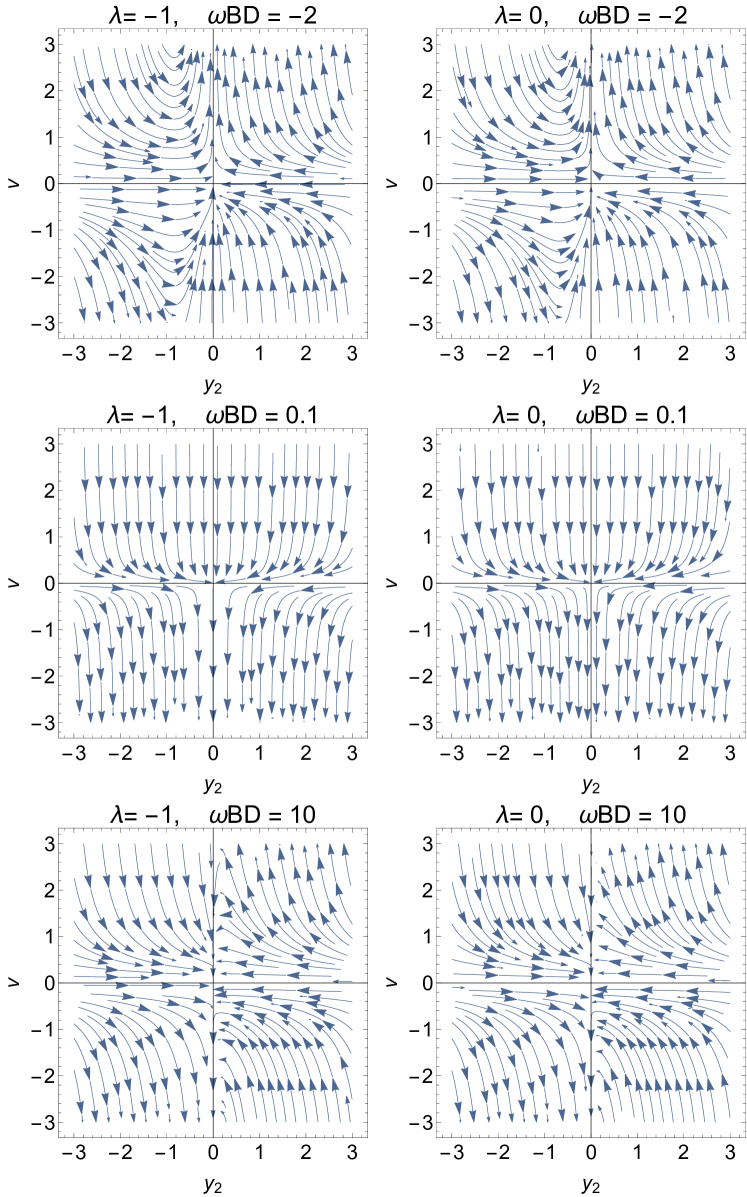
Figure 1: Phase plot of the dynamical system (57), where it is shown that the origin is unstable (saddle point).

IV.1.2 Case $\lambda=4$

Consider now the case $\lambda=4$. The specific model can describe a cosmological history with at least two acceleration phases, a matter epoch and a radiation era. That is an interesting result as it can describe the important eras of cosmological evolution. Note that $\lambda=4$ corresponds to potential $V\left(\psi\right)=V_{0}\psi^{4},$ and for the original scalar field $\phi$, the potential function $V\left(\phi\right)=V_{0}\phi^{2}$.

Now, for $\lambda=4$, the similarity matrix is given by

$$s=\left(\begin{array}[]{cccc}0&0&-\frac{1}{2}&0\\ -\frac{3\bar{\omega}_{BD}}{2}&0&1&0\\ 1&1&0&0\\ 0&0&0&1\\ \end{array}\right).$$ (62)

Introduce the linear transformation

$$\left(\begin{array}[]{c}v\\ y_{1}\\ y_{2}\\ y_{3}\end{array}\right)=\left(\begin{array}[]{c}\mu\\ -\frac{2(2x+y+1)}{3\bar{\omega}_{BD}}\\ \frac{2(2x+y+1)}{3\bar{\omega}_{BD}}+z\\ -2x\end{array}\right),$$ (63)

we obtain the system

$$\frac{dv}{d\tau}=3y_{1}v^{2}+3y_{2}v^{2}-\frac{y_{3}v}{2},$$ (64)

$$\frac{dy_{1}}{d\tau}=-6y_{1}+y_{1}^{2}(-6y_{3}v-18v-9\bar{\omega}_{BD})$$

$$+y_{1}\left(-6y_{2}y_{3}v+y_{3}^{2}\left(v\left(\frac{2}{\bar{\omega}_{BD}}+\frac{1}{4}\right)+\frac{1}{2}\right)+y_{3}\left(\frac{6v}{\bar{\omega}_{BD}}+6\right)\right)+\frac{2y_{2}y_{3}^{2}v}{\bar{\omega}_{BD}}$$

$$+y_{3}^{3}\left(-\frac{v}{12\bar{\omega}_{BD}}-\frac{1}{6\bar{\omega}_{BD}}\right),$$ (65)

$$\frac{dy_{2}}{d\tau}=-3y_{2}+y_{1}^{2}\left(3y_{3}v+9v+\frac{9\bar{\omega}_{BD}}{2}\right)$$

$$+y_{1}\Bigg{(}y_{2}\left(-9v-\frac{9\bar{\omega}_{BD}}{2}\right)+y_{3}^{2}\left(v\left(-\frac{2}{\bar{\omega}_{BD}}-\frac{1}{8}\right)-\frac{1}{4}\right)$$

$$+y_{3}\left(v\left(\frac{1}{2}-\frac{12}{\bar{\omega}_{BD}}\right)-\frac{7}{2}\right)+v\left(\frac{3}{2}-\frac{18}{\bar{\omega}_{BD}}\right)\Bigg{)}-3y_{2}^{2}y_{3}v$$

$$+y_{2}\left(y_{3}^{2}\left(v\left(\frac{1}{8}-\frac{2}{\bar{\omega}_{BD}}\right)+\frac{1}{4}\right)+y_{3}\left(v\left(\frac{1}{2}-\frac{6}{\bar{\omega}_{BD}}\right)+\frac{5}{2}\right)\right)$$

$$+y_{3}^{3}\left(\frac{v}{12\bar{\omega}_{BD}}+\frac{1}{6\bar{\omega}_{BD}}\right)+y_{3}^{2}\left(v\left(\frac{1}{4\bar{\omega}_{BD}}-\frac{1}{48}\right)+\frac{1}{2\bar{\omega}_{BD}}\right),$$ (66)

$$\frac{dy_{3}}{d\tau}=-3y_{3}+y_{1}\left(-3y_{3}^{2}v+y_{3}\left(-3v-\frac{9\bar{\omega}_{BD}}{2}\right)+18v\right)+y_{2}\left(6y_{3}v-3y_{3}^{2}v\right)$$

$$+y_{3}^{3}\left(\frac{v}{8}+\frac{1}{4}\right)+y_{3}^{2}\left(\frac{5}{2}-\frac{v}{4}\right).$$ (67)

Applying the procedure to find the center manifold to (64), (65), (66), (67), we obtain that the dynamics on the center manifold of $P_{3}$ is governed by

$$\frac{dv}{d\tau}=0.$$ (68)

Therefore, we rely on numerical inspection. For example, in the invariant set $y_{1}=y_{3}=0$ the dynamics is given by

$$y_{2}^{\prime}=-3y_{2},\quad v^{\prime}=3v^{2}y_{2}.$$ (69)

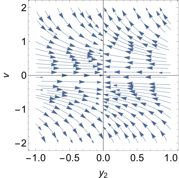
Figure 2: Phase plot of the dynamical system (69), wherein it is shown that the origin is unstable (saddle point).

In figure 2 a phase plot of the dynamical system (69) is presented, where it is shown that the origin is unstable (saddle point).

V Nonzero spatial curvature

We now assume the presence of nonzero spatial curvature, that is, the background space is described by the line element

$$ds^{2}=-dt^{2}+a^{2}\left(t\right)\left(\frac{dr^{2}}{1-Kr^{2}}+r^{2}\left(d\theta^{2}+\sin^{2}\theta d\phi^{2}\right)\right).$$ (70)

The parameter $K$ denotes the curvature for the three-dimensional hypersurface. For a closed FLRW universe $K=+1$, while for an open FLRW universe $K=-1$.

For a nonzero $K$ the cosmological field equations are modified as follows

$$6H^{2}+12H\left(\frac{\dot{\psi}}{\psi}\right)+\frac{\bar{\omega}_{BD}}{2}\left(\dot{\psi}^{2}+2\beta\hbar^{2}\left(\frac{\dot{\psi}}{\psi}\right)\left(\frac{\dot{\zeta}}{\psi}\right)-\frac{\zeta^{2}}{\psi^{2}}\right)+\frac{V\left(\psi\right)}{\psi^{2}}-6K\frac{\psi^{2}}{a^{2}}=0,$$ (71)

$$2\dot{H}+3H^{2}+4\left(\frac{\dot{\psi}}{\psi}\right)H+\left(\frac{\bar{\omega}_{BD}}{4}-2\right)\left(\frac{\dot{\psi}}{\psi}\right)^{2}+2\left(\frac{\ddot{\psi}}{\psi}\right)+\frac{V\left(\psi\right)}{2\psi^{2}}+\beta\frac{\bar{\omega}_{BD}}{4\psi^{2}}\left(\zeta^{2}-2\dot{\zeta}\dot{\psi}\right)-2K\frac{\psi^{2}}{a^{2}}=0,$$ (72)

$$\ddot{\psi}+3H\dot{\psi}+\zeta=0,$$ (73)

$$\bar{\omega}_{BD}\left(\beta\ddot{\zeta}+\ddot{\psi}\right)+3\bar{\omega}_{BD}H\left(\beta\dot{\zeta}+\dot{\psi}\right)+V_{,\psi}+12\psi\left(\dot{H}+2H^{2}-Ka^{-2}\right)=0.$$ (74)

In order to proceed with the analysis of the dynamical evolution and the investigation of the stationary points for the latter system we define the new set of variables kkd1

$$X=\frac{\dot{\psi}}{\psi\sqrt{H^{2}+\left|K\right|a^{-2}}}~{},~{}Y=\frac{V\left(\psi\right)}{6\psi^{2}\left(H^{2}+\left|K\right|a^{-2}\right)}~{},~{}Z=\beta\hbar^{2}\frac{\dot{\zeta}}{6\psi^{2}\sqrt{H^{2}+\left|K\right|a^{-2}}}~{}~{},$$ (75)

$$W=\beta\hbar^{2}\frac{\zeta^{2}}{12\psi^{2}\sqrt{H^{2}+\left|K\right|a^{-2}}}~{},~{}\eta=\frac{H}{\sqrt{H^{2}+\left|K\right|a^{-2}}}~{},~{}\lambda=\psi\frac{V_{,\psi}\left(\psi\right)}{V\left(\psi\right)}~{},$$ (76)

$$\mu=-\frac{1}{\beta}\frac{\psi}{\zeta}~{},~{}\Gamma\left(\lambda\right)=\frac{V_{,\psi\psi}\left(\psi\right)V\left(\psi\right)}{\left(V_{,\psi}\left(\psi\right)\right)^{2}}.$$

In the following we consider the two cases, $K=+1$ and $K=-1$.

V.1 Closed Universe

For a positive curvature term, i.e. $K=+1$, and for the new independent variable $d\sigma=\sqrt{H^{2}+\left|K\right|a^{-2}}dt$, the field equations in the dimensionless variables are

$$8\frac{dX}{d\sigma} =48\mu W-4\eta X\left(2\eta^{2}+3W(4\mu+\text{$\bar{\omega}_{BD}$})+3Y-5\right)$$

$$+(\text{$\bar{\omega}_{BD}$}-8)\eta X^{3}-4X^{2}\left(2\eta^{2}-3\text{$\bar{\omega}_{BD}$}\eta z+2\right),$$ (77)

$$\frac{4}{Y}\frac{dY}{d\sigma} =-4\eta\left(2\eta^{2}+3W(4\mu+\text{$\bar{\omega}_{BD}$})+3Y+1\right)$$

$$+(\text{$\bar{\omega}_{BD}$}-8)\eta X^{2}+4X\left(\lambda-2\eta^{2}+3\text{$\bar{\omega}_{BD}$}\eta Z-2\right),$$ (78)

$$-\text{$\bar{\omega}_{BD}$}\frac{dZ}{d\sigma} =-4W(-2(\text{$\bar{\omega}_{BD}$}-12)\mu-3\text{$\bar{\omega}_{BD}$}\eta Z(4\mu+\text{$\bar{\omega}_{BD}$})+6\text{$\bar{\omega}_{BD}$})$$

$$+4X\left(-4\eta-3\text{$\bar{\omega}_{BD}$}^{2}\eta Z^{2}+2\text{$\bar{\omega}_{BD}$}\left(\eta^{2}+4\right)Z\right)$$

$$+(\text{$\bar{\omega}_{BD}$}-8)X^{2}(2-\text{$\bar{\omega}_{BD}$}\eta Z)+8\left(2\eta^{2}+(\lambda-3)Y-1\right)$$

$$+4\text{$\bar{\omega}_{BD}$}\eta Z\left(2\eta^{2}+3Y-5\right),$$ (79)

$$\frac{4}{W}\frac{dW}{d\sigma} =4\left(-\eta\left(2\eta^{2}+3W(4\mu+\text{$\bar{\omega}_{BD}$})+3Y+1\right)-6\mu Z\right)$$

$$+(\text{$\bar{\omega}_{BD}$}-8)\eta X^{2}-4X\left(2\eta^{2}-3\text{$\bar{\omega}_{BD}$}\eta Z+2\right),$$ (80)

$$\frac{8}{\left(\eta^{2}-1\right)}\frac{d\eta}{d\sigma}=\left(8\eta^{2}+12W(4\mu+\text{$\bar{\omega}_{BD}$})-X(-8\eta+(\text{$\bar{\omega}_{BD}$}-8)X+12\text{$\bar{\omega}_{BD}$}Z)+12y-4\right),$$ (81)

$$\frac{d\lambda}{d\sigma}=\lambda x\left(1-\lambda\left(1-\Gamma\left(\lambda\right)\right)\right),$$ (82)

$$\frac{d\mu}{d\sigma}=\mu\left(x+3z\mu\right),$$ (83)

with constraint

$$12\left(Y+2\eta^{2}-1\right)-24X\eta-12\bar{\omega}_{BD}W+\bar{\omega}_{BD}x\left(X+12Z\right)=0.$$ (84)

As before for the scalar field potential we consider the power-law potential function in which $\lambda=const$.

By using the algebraic equation (84) the stationary points for the positive curvature are derived to be of the form $\mathbf{A}=\left(X\left(A\right),Y\left(A\right),Z\left(A\right),\mu\left(A\right),\eta\left(A\right)\right)$. Indeed the stationary points are

$$A_{1}^{\pm}=\left(\pm 1,0,Z_{1},\pm 1\right),~{}A_{2}^{\pm}=\left(\pm\frac{6}{\lambda},\frac{2}{\lambda^{2}}\left(\lambda-6\right),Z_{2},\pm 1\right),$$

$$A_{3}^{\pm}=\left(0,-1,\frac{\lambda-4}{3\bar{\omega}_{BD}},\pm 1\right)~{},~{}A_{4}^{\pm}=\left(\pm 1,0,\pm\left(\frac{1}{12}-\frac{1}{\bar{\omega}_{BD}}\right),\frac{4\bar{\omega}_{BD}}{\bar{\omega}_{BD}-4},\pm 1\right),$$

$$A_{5}^{\pm}=\left(\pm\frac{6}{\lambda},\frac{2}{\lambda^{2}}\left(\lambda-6\right),\mp\frac{\lambda\left(\lambda-10\right)+3\left(\bar{\omega}_{BD}-4\right)}{6\bar{\omega}_{BD}\lambda},\frac{12\bar{\omega}_{BD}}{\lambda\left(\lambda-10\right)+3\left(\bar{\omega}_{BD}-4\right)},\pm 1\right),$$

$$A_{6}^{\pm}=\left(X_{6},0,-\frac{2}{\bar{\omega}_{BD}}\left(\mp 2+\frac{1}{X_{6}}\right)-\frac{X_{6}}{6},\frac{2\bar{\omega}_{BD}X_{6}^{2}}{12+X_{6}\left(\mp 24+\bar{\omega}_{BD}X_{6}\right)}\pm 1\right),$$

$$A_{7}^{\pm}=\left(0,0,0,\mu,\pm\frac{\sqrt{2}}{2}\right),~{}A_{8}^{\pm}=\left(\pm\sqrt{2},0,Z_{9},0,\pm\frac{\sqrt{2}}{2}\right),$$

$$A_{9}^{\pm}=\left(\pm\sqrt{2},0,\frac{\bar{\omega}_{BD}-12}{6\sqrt{2}\bar{\omega}_{BD}},\frac{4\bar{\omega}_{BD}}{\bar{\omega}_{BD}-12},\pm\frac{\sqrt{2}}{2}\right).$$

For each stationary point we calculate the equation of state parameter $w_{tot}=-1-\frac{2}{3}\frac{\dot{H}}{H}$ and the deceleration parameter $q=\frac{1}{2}\left(1+3w_{tot}\right)\left(1+\frac{K}{a^{2}H^{2}}\right)$.

Stationary points, $A_{1}^{\pm}$, $A_{2}^{\pm}$, $A_{3}^{\pm}$, $A_{4}^{\pm}$ and $A_{5}^{\pm}$, describe spatially flat asymptotic solutions as described by the stationary points $P_{1}$, $P_{2}$, $P_{3}$, $P_{4}$ and $P_{5}$, respectively. For the points $A_{6}^{\pm}$ we derive $w_{tot}\left(A_{6}^{\pm}\right)=\frac{1}{3}\left(3+2X_{6}\left(X_{6}\mp 2\right)\right)$ and $q\left(A_{6}^{\pm}\right)=2\left(1\mp X_{6}\right)$. Consequently, $A_{6}^{\pm}$ describe asymptotic solutions with curvature. For the point $A_{6}^{+}$ the scale factor is exponential when $X_{6}=1\pm\frac{\sqrt{10}}{2}$.

Table 2: Stationary points for the modified Brans-Dicke cosmological model with positive curvature.

Point	$\mathbf{w}_{tot}\left(\mathbf{A}\right)$	Curvature	Stability
$A_{1}^{\pm}$	$\frac{1}{3}$	Flat	Saddle
$A_{2}^{\pm}$	$1-\frac{4}{\lambda}$	Flat	Saddle
$A_{3}^{\pm}$	$-1$	Flat	Saddle
$A_{4}^{\pm}$	$\frac{1}{3}$	Flat	Saddle
$A_{5}^{\pm}$	$1-\frac{4}{\lambda}$	Flat	Saddle
$A_{6}^{\pm}$	$\frac{1}{3}\left(3+2X_{6}\left(X_{6}\mp 2\right)\right)$	$K>0$	Saddle
$A_{7}^{\pm}$	$-\frac{1}{3}$	$K>0$	Saddle
$A_{8}^{\pm}$	$-\frac{1}{3}$	$K>0$	Saddle
$A_{9}^{\pm}$	$-\frac{1}{3}$	$K>0$	$A_{9}^{+}$ attractor for $\lambda<3$

The asymptotic solutions at the stationary points $A_{7}^{\pm}$, $~{}A_{8}^{\pm}$ and $~{}A_{9}^{\pm}$ are that with $w_{tot}=-\frac{1}{3}$ and $q=0$. Hence, at the points the asymptotic solutions describe spacetimes with nonzero spatial curvature.

We calculate the eigenvalues for the linearized system in order to study the stability properties for the stationary points.

The linearized system around the points $A_{1}^{\pm}$ gives the eigenvalues $e_{2}\left(A_{1}^{\pm}\right)=0$ , $e_{2}\left(A_{1}^{\pm}\right)=\pm 1$ , $e_{3}\left(A_{1}^{\pm}\right)=\mp 1~{}$, $e_{4}\left(A_{1}^{\pm}\right)=\pm 2$  and $e_{5}\left(A_{1}^{\pm}\right)=\pm\left(\lambda-6\right).~{}$Therefore, the solutions at the points $A_{1}^{\pm}$ are always unstable and $A_{1}^{\pm}$ are saddle points.

The eigenvalues of the stationary points $A_{2}^{\pm}$ are derived to be $e_{1}\left(A_{2}^{\pm}\right)=0$,$~{}e_{2}\left(A_{2}^{\pm}\right)=\pm\frac{6}{\lambda}$,$~{}e_{3}\left(A_{2}^{\pm}\right)=\pm\left(4-\frac{12}{\lambda}\right)~{}$, $e_{4}\left(A_{2}^{\pm}\right)=\mp\frac{3}{\lambda}\left(1+\sqrt{25-4\lambda}\right)$ and $e_{5}\left(A_{2}^{\pm}\right)=\frac{3}{\lambda}\left(1+\sqrt{25-4\lambda}\right)$. Consequently, $A_{2}^{\pm}$ are saddle points.

For points $A_{3}^{\pm}$ the eigenvalues are $e_{1}\left(A_{3}^{\pm}\right)=0$ , $e_{2}\left(A_{3}^{\pm}\right)=\pm 3$, $e_{3}\left(A_{3}^{\pm}\right)=\pm 3$, $e_{4}\left(A_{3}^{\pm}\right)=\mp 2$, $e_{5}\left(A_{3}^{\pm}\right)=\pm 6$. Hence points $A_{3}^{\pm}$ are saddle points.

Similarly for the  points $~{}A_{4}^{\pm}$ we derive $e_{1}\left(A_{4}^{\pm}\right)=\mp 1$, $~{}e_{2}\left(A_{4}^{\pm}\right)=\mp 1$, $e_{3}\left(A_{4}^{\pm}\right)=\pm 2\,$  $e_{4}\left(A_{4}^{\pm}\right)=\mp 2$, $e_{5}\left(A_{4}^{\pm}\right)=\pm\left(\lambda-6\right)~{}$, that is, $A_{4}^{\pm}$ are saddle points.

The linearized system around points $A_{5}^{\pm}$ are $e_{1}\left(A_{5}^{\pm}\right)=\mp\frac{6}{\lambda}$ , $e_{2}\left(A_{5}^{\pm}\right)=\pm\left(4-\frac{12}{\lambda}\right)$, $e_{3}\left(A_{5}^{\pm}\right)=\mp\frac{12}{\lambda}$ and $e_{4}\left(A_{5}^{\pm}\right)=\mp\frac{3}{\lambda}\left(1+\sqrt{\left(25-4\lambda\right)}\right)~{},~{}e_{5}\left(A_{5}^{\pm}\right)=\mp\frac{3}{\lambda}\left(1-\sqrt{\left(25-4\lambda\right)}\right)$, that is, the solutions at points $A_{5}^{\pm}$ are always unstable. Points $A_{5}^{\pm}$ are always saddle points.

The eigenvalues of points $A_{6}^{\pm}$ are derived to be $e_{1}\left(A_{6}^{\pm}\right)=0$, $e_{2}\left(A_{6}^{\pm}\right)=-4\left(X_{6}\mp 1\right)$, $e_{3}\left(A_{6}^{\pm}\right)=\left(2+\lambda\right)X_{6}\mp 6$, $e_{4}\left(A_{6}^{\pm}\right)=X_{6}\sqrt{\frac{X_{6}\left(\pm 48+\left(\bar{\omega}_{BD}-36\right)X_{6}\right)-24}{X_{6}\left(\bar{\omega}_{BD}\mp 24\right)+12}}$, $e_{5}\left(A_{6}^{\pm}\right)=-X_{6}\sqrt{\frac{X_{6}\left(\pm 48+\left(\bar{\omega}_{BD}-36\right)X_{6}\right)-24}{X_{6}\left(\bar{\omega}_{BD}\mp 24\right)+12}}$. Thus, the stationary points $A_{6}^{\pm}$ are saddle points.

For the points $A_{7}^{\pm}$ two of eigenvalues are $e_{1}\left(A_{7}^{\pm}\right)=\sqrt{2}$ , $e_{2}\left(A_{7}^{\pm}\right)=-\sqrt{2}$, from where we infer that $A_{7}^{\pm}$ are always saddle points.

The five eigenvalues for the linearized system around points $A_{8}^{\pm}~{}$are $e_{1}\left(A_{8}^{\pm}\right)=0$, $e_{2}\left(A_{8}^{\pm}\right)=\sqrt{2}~{}$, $e_{1}\left(A_{8}^{\pm}\right)=-\sqrt{2}$, $e_{2}\left(A_{8}^{\pm}\right)=\mp 2\sqrt{2}\,$, $e_{1}\left(A_{8}^{\pm}\right)=\pm\sqrt{2}\left(\lambda-3\right)$, which means that points  $A_{8}^{\pm}$ are saddle points.

The eigenvalues of the linearized system around $A_{9}^{\pm}$ are $e_{1}\left(A_{9}^{\pm}\right)=\mp\sqrt{2}$,$~{}e_{2}\left(A_{9}^{\pm}\right)=\mp\sqrt{2}$, $e_{3}\left(A_{9}^{\pm}\right)=\mp 2\sqrt{2}$, $e_{4}\left(A_{9}^{\pm}\right)=\mp 2\sqrt{2}$, $e_{5}\left(A_{9}^{\pm}\right)=\mp\sqrt{2}\left(3-\lambda\right)$, that is, point $A_{9}^{+}$ is an attractor for $\lambda<3$, while point $A_{9}^{+}$ is a source for $\lambda<3$, otherwise is a saddle point. The results are summarized in Table 2.

V.2 Open Universe

For a negative curvature FLRW background space the field equations in the dimensionless variables are

$$\frac{dX}{d\sigma} =6\mu W-\frac{3}{2}\eta X(W(4\mu+\text{$\bar{\omega}_{BD}$})+Y-1)$$

$$+\frac{1}{8}(\text{$\bar{\omega}_{BD}$}-8)\eta X^{3}-\frac{1}{2}X^{2}\left(2\eta^{2}-3\text{$\bar{\omega}_{BD}$}\eta Z+2\right),$$ (85)

$$\frac{4}{Y}\frac{dY}{d\sigma} =-12\eta(W(4\mu+\text{$\bar{\omega}_{BD}$})+Y+1)$$

$$+(\text{$\bar{\omega}_{BD}$}-8)\eta X^{2}+4X\left(\lambda-2\eta^{2}+3\text{$\bar{\omega}_{BD}$}\eta Z-2\right),$$ (86)

$$-8\bar{\omega}_{BD}\frac{dZ}{d\sigma} =-4W(-2(\text{$\bar{\omega}_{BD}$}-12)\mu-3\text{$\bar{\omega}_{BD}$}\eta Z(4\mu+\text{$\bar{\omega}_{BD}$})+6\text{$\bar{\omega}_{BD}$})$$

$$+4X\left(-4\eta-3\text{$\bar{\omega}_{BD}$}^{2}\eta Z^{2}+2\text{$\bar{\omega}_{BD}$}\left(\eta^{2}+4\right)Z\right)+(\text{$\bar{\omega}_{BD}$}-8)X^{2}(2-\text{$\bar{\omega}_{BD}$}\eta Z)$$

$$+8(\lambda-3)Y+12\text{$\bar{\omega}_{BD}$}\eta(Y-1)Z+8,$$ (87)

$$\frac{4}{W}\frac{dW}{d\sigma} =12(-\eta(W(4\mu+\text{$\bar{\omega}_{BD}$})+Y+1)-2\mu Z)+(\text{$\bar{\omega}_{BD}$}-8)\eta X^{2}$$

$$-4X\left(2\eta^{2}-3\text{$\bar{\omega}_{BD}$}\eta Z+2\right),$$ (88)

$$\frac{d\lambda}{d\sigma} =\lambda x\left(1-\lambda\left(1-\Gamma\left(\lambda\right)\right)\right),$$ (89)

$$\frac{d\mu}{d\sigma} =\mu\left(x+3z\mu\right),$$ (90)

$$\frac{d\eta}{d\sigma} =\frac{1}{8}\left(\eta^{2}-1\right)(12W(4\mu+\text{$\bar{\omega}_{BD}$})$$

$$-X(-8\eta+(\text{$\bar{\omega}_{BD}$}-8)x+12\text{$\bar{\omega}_{BD}$}Z)+12Y+4).$$ (91)

Furthermore, the algebraic constraint equation is

$$12\left(1+Y\right)+\bar{\omega}_{BD}X\left(X+12Z\right)-24X\eta-12\bar{\omega}_{BD}W=0.$$ (92)

For the power-law potential for which $\lambda=const$, the stationary points in the five-dimensional space $\left(X,Y,Z,\mu,\eta\right)$ are points $A_{1}^{\pm}$, $A_{2}^{\pm}$, $A_{3}^{\pm}$, $A_{4}^{\pm}$, $A_{5}^{\pm}~{}$and $A_{6}^{\pm}$.   The physical properties of the points are the same as those for positive curvature, as also the stability properties. What is more important to mention here is that the Milne solution sm1 is not provided by the GUP modified Brans-Dicke model. That is not an unexpected result. Milne solution is the vacuum solution of General Relativity, but because of the nature of coupling of the scalar field with the gravitational field a zero contribution of the scalar field in the field equations is not allowed.

VI Conclusions

In this piece of work we proposed a modified Brans-Dicke cosmological model inspired by the minimum length uncertainty. Specifically, in the Brans-Dicke Action Integral the kinetic part of the scalar field has been modified in order that the equation of motion for the scalar field be given by the quadratic GUP. New higher-order derivative terms for the scalar field have been introduced in the gravitational Action Integral. With the use of a Lagrange multiplier the higher-order derivative terms have been attributed to a new scalar field with nonzero interaction terms with the Brans-Dicke field.

We calculated the cosmological field equations for the a homogeneous and isotropic background space, described by the FLRW metric. In order to investigate the effects of the higher-order terms provided by GUP in the cosmological evolution we considered dimensionless variables in the context of the $H$-normalization and we determined the stationary points and their stability properties. We perform our analysis for the spatially flat FLRW universe as also in the presence of a nonzero spatial curvature.

We compare the results for the modified Brans-Dicke theory with that of the unmodified theory, where we observe that the new degrees of freedom given by GUP change dramatically the dynamics and the provided asymptotic solutions for the field equations. Specifically, for the case of a power-law potential function we found that more than one acceleration phases are provided by the theory, as also an asymptotic solution which describes the radiation era is always present. The physical properties of the stationary points depend upon on the exponent of the potential function and not on the value of the Brans-Dicke parameter, in contrary to the unmodified model.

This analysis is based on a series of studies where we consider the modification of the scalar field Lagrangian inspired by the GUP. In previous studies we consider the quintessence model while here we assume the Brans-Dicke theory. It both cases we found that the higher-order terms provided by GUP affects the dynamics such that more acceleration asymptotic solutions to be provided in the cosmological dynamics. In addition, the de Sitter universe is provided as an asymptotic solutions for the both theories, either for scalar field potentials where the de Sitter universe does not exist for the unmodified scalar field theories.

References

• (1) T. Clifton, P.G. Ferreira, A. Padilla and C. Skordis, Physics Rept. 1, 513 (2012)
• (2) B. Ratra and P.J.E Peebles, Phys. Rev. D 37 3406 (1988)
• (3) E.V Linder, Phys. Rev. D. 70 023511 (2004)
• (4) P. Christodoulidis, D. Roest and E.I. Sfakianakis, JCAP 12, 059 (2019)
• (5) P. Horava, Phys. Rev. D 79, 084008 (2009)
• (6) S. Kanno and J. Soda, Phys. Rev. D 74, 063505 (2006)
• (7) O. Bertolami and P.J. Martins, Phys. Rev. D 61, 064007 (2000)
• (8) J.D. Barrow and A.C. Ottewill, J. Phys. A 16, 2757 (1983)
• (9) H.A. Buchdahl, Mon. Not. Roy. Astron. Soc. 150, 1 (1970)
• (10) T. Harko, F.S.N. Lobo, S. Nojiri and S.D. Odintsov, Phys. Rev. D 84, 024020 (2011)
• (11) R. Ferraro and F. Fiorini, Phys. Rev. D 75, 084031 (2007)
• (12) S. Bahamonde, C. G. Bohmer and M. Wright, Phys. Rev. D 92, 104042 (2015)
• (13) A. Paliathanasis, JCAP 1708, 027 (2017)
• (14) T. Clifton and J.D. Barrow, Class. Quant. Grav. 23, 2951 (2006)
• (15) T.P. Sotiriou and V. Faraoni Rev. Mod. Phys. 82, 451 (2010)
• (16) S. Nojiri and S.D. Odintsov, Phys. Rep. 505, 59 (2011)
• (17) T.P. Sotiriou, Gravity and Scalar Fields, Modifications of Einstein’s Theory of Gravity at Large Distances ed. E. Papantonopoulos, Lecture Notes in Physics, vol 892. Springer, (2015)
• (18) G. Leon and F.O. Franz Silva, Class. Quantum Grav. 38, 015004 (2020)
• (19) G. Leon, A. Paliathanasis and J.L. Morales-Martinez, EPJC 78, 753 (2018)
• (20) L. Amendola, D. Polarski and S. Tsujikawa, Phys. Rev. Lett. 98, 131302 (2007)
• (21) L.J. Garay, Int. J. Mod. Phys. A 10, 145 (1995)
• (22) R. Casadio, O. Micu and P. Nicolini, Minimum Length Effects in Black Hole Physics, Quantum Aspects of Black Holes ed. X. Camlent, Fundamental Theories of Physics, 178. Springer, Cham (2015)
• (23) L.N. Chang, Z. Lewis, D. Mimic and T. Takeuchi, Advances in High Energy Physics 2011, 4935514 (2011)
• (24) C. Nassif, Int. J. Mod. Phys. D 19, 539 (2010)
• (25) J. Greensite, Phys. Lett. B 255, 375 (1991)
• (26) M. Maggiore, Phys. Lett. B 304, 65 (1993)
• (27) A. Camelia, Int. J. Mod. Phys. D 11, 35 (2002)
• (28) A.F. Ali, S. Das, E.C. Vagenas, Phys. Lett. B 678, 497 (2009)
• (29) Z. Silagadge, Phys. Lett. A 373, 2643 (2009)
• (30) E.C. Vagenas, A.F. Ali, M. Hemeda and H. Alshal, EPJC 79, 398 (2019)
• (31) F. Lu, J. Tao and P. Wang, JCAP 12, 036 (2018)
• (32) R. Casadio and F. Scardigli, Phys. Lett. B 807, 135558 (2020)
• (33) R.J. Adler, P. Chen and D.I. Santiago, Gen. Rel. Gravit. 33, 2101 (2001)
• (34) A. Paliathanasis and M. Tsamparlis, J. Geom. Phys. 107, 45 (2016)
• (35) Y.-G. Miao and Y.-J. Zhao, Int. J. Phys. D. 23, 1450062 (2014)
• (36) R.Garattini and M. Faizal, Nucl. Phys. B 905, 313 (2016)
• (37) A.M. Diab and A.N. Tawfik, Astron. Nachr. 342, 49 (2021)
• (38) K. Zeynali, F. Darabi and H. Motavalli, JCAP 12, 033 (2012)
• (39) L.N. Chang, D. Minic, N. Okamura and T. Takeuchi, Phys. Rev D 65, 125028 (2002)
• (40) A. Paliathanasis, S. Pan and S. Pramanik, Class. Quantum Grav. 32, 245006 (2015)
• (41) A. Giacomini, G. Leon, A. Paliathanasis and S. Pan, EPJC 80, 931 (2020)
• (42) A. Paliathanasis, G. Leon, W. Khyllep, J. Dutta and S. Pan, EPJC 81, 607 (2021)
• (43) C. Brans and R.H. Dicke, Phys. Rev. 124 195 (1961)
• (44) H. Bondi and J. Samuel, Phys. Lett. A 228, 121 (1997)
• (45) E. Gasco, Mach’s Principle: the original Einstein’s considerations (1907-12). Il Principio di Mach: le prime considerazioni di Einstein (1907-12), Italian Physical Society 13, 75 (2005)
• (46) V. Faraoni, Phys. Rev. D 59, 084021, (1999)
• (47) J. O’Hanlon, Phys. Rev. Lett. 29 137 (1972)
• (48) T.P. Sotiriou, Gravity and Scalar fields, Proceedings of the 7th Aegean Summer School: Beyond Einstein’s theory of gravity, Modifications of Einstein’s Theory of Gravity at Large Distances, Paros, Greece, ed. by E. Papantonopoulos, Lect.Notes Phys. 892, (2015).
• (49) V. Faraoni, Cosmology in Scalar-Tensor Gravity, Fundamental Theories of Physics vol. 139, Kluwer Academic Press: Netherlands (2004)
• (50) M. Tsamparlis, A. Paliathanasis, S. Basilakos and S. Capozziello, Gen. Rel. Grav. 45, 2003 (2013)
• (51) R. E. Morganstern, Phys. Rev. D 4, 946 (1971)
• (52) O. Obregn and P. Chauvet, Astroph. Space Sci. 56, 335 (1978)
• (53) V. Faraoni, Fundam. Theor. Phys. 139 (2004)
• (54) A. Paliathanasis, M. Tsamparlis, S. Basilakos and S. Capozziello, Phys. Rev. D 93, 043528 (2016)
• (55) G. Papagiannopoulos, J.D. Barrow, S. Basilakos, A. Giacomini and A. Paliathanasis, Phys. Rev. D 95, 024021 (2017)
• (56) R.E. Morganstern, Phys. Rev. D 4, 282 (1971)
• (57) A. E. Montenegro Jr. and S. Carneiro, Class. Quantum Grav. 24, 313 (2007)
• (58) V.B. Johri and G.K. Goswami, J. Math. Phys. 21, 2269 (1980)
• (59) B. Chauvineau, J. Math. Phys. 43, 1487 (2002)
• (60) A. Paliathanasis, M. Tsamparlis, S. Basilakos and J.D. Barrow, Phys. Rev. D 93, 043528 (2016)
• (61) O. Hrycyna and M. Szydlowski, JCAP 12, 016 (2013)
• (62) A. Cid, G. Leon and Y. Leyva, JCAP 16, 027 (2016)
• (63) G. Leon, A. Paliathanasis and L. Velazquez, Gen. Rel. Grav. 52, 71 (2020)
• (64) C. Quesne and V.M. Tkachuk, J. Phys. A 39, 10909 (2006)
• (65) S. Das and E.C. Vagenas, Phys. Rev. Lett. 101, 221301 (2008)
• (66) A. Kempf, J. Phys. A: Math. Gen. 30, 2093 (1997)
• (67) H. Hinrichen and A. Kempf, J. Math. Phys. 37, 2121 (1996)
• (68) P. Jizba, H. Kleinert and F. Scardigli, Phys. Rev. D 81, 084030 (2010).
• (69) L. Buoninfante, G.G. Luciano and L. Petruzziello, EPJC 79, 663 (2019).
• (70) F. Scardigli, G. Lambiase and E. Vagenas, Phys. Lett. B 767, 242 (2012).
• (71) L. Buoninfante, G. Lambiase, G.G. Luciano and L. Petruzziello, EPJC 80, 853 (2020)
• (72) P. Pedram, Phys. Lett. B 718, 638 (2012)
• (73) E.C. Vagenas, A.F. Ali, M. Hemeda and H. Alshal, EPJC 79, 398 (2019)
• (74) S. Aghababaei, H. Moradpour and E.C. Vagenas, Eur. Phys. J. Plus 136, 997 (2021)
• (75) H. Shababi and W.S. Chung, Phys. Lett. B 770, 445 (2017)
• (76) A. Paliathanasis, S. Pan and S. Pramanik, Class. Quantum Grav. 32, 245006 (2015)
• (77) A. Giacomini, G. Leon, A. Paliathanasis and S. Pan, EPJC 80, 931 (2020)
• (78) Y.-G. Miao and Y.-J. Zhao, Int. J. Mod. Phys. D. 23, 1450062 (2014)
• (79) A.M. Diab and A.N. Tawfik, Aston. Nachr. 342, 49 (2021)
• (80) M. Kerachian, G. Acquaviva and G. Lukes-Gerakopoulos, Phys. Rev. D 101, 043535 (2020)
• (81) M.P. Dabrowski, T. Denkiewicz and D. Blaschke, Annalen Phys. 16, 237 (2007)
• (82) L. Perko, Differential Equations and Dynamical Systems  Springer-Verlag, New York, 1991.
• (83) J. Guckenheimer and P. Holmes, Nonlinear Oscillations, Dynamical Systems and Bifurcations of Vector Fields  SpringerVerlag, New York, 1983.