A Kernel-Based Approach for Modelling Gaussian Processes with Functional Information

Abstract

Gaussian processes are among the most useful tools in modeling continuous processes in machine learning and statistics. If the value of a process is known at a finite collection of points, one may use Gaussian processes to construct a surface which interpolates these values to be used for prediction and uncertainty quantification in other locations. However, it is not always the case that the available information is in the form of a finite collection of points. For example, boundary value problems contain information on the boundary of a domain, which is an uncountable collection of points that cannot be incorporated into typical Gaussian process techniques. In this paper we construct a Gaussian process model which utilizes reproducing kernel Hilbert spaces to unify the typical finite case with the case of having uncountable information by exploiting the equivalence of conditional expectation and orthogonal projections. We discuss this construction in statistical models, including numerical considerations and a proof of concept.

1 Introduction

Gaussian processes (GPs; Rasmussen et al., 2006) are popular tools among statisticians and engineers for modeling complex problems because of their flexibility, simplicity, and their ability to quantify uncertainty. As Gaussian processes have become more popular in practice, there is an increased demand to modify Gaussian processes to possess certain characteristics. Swiler et al. (2020) give several such possibilities to implement bound constraints, monotonicity constraints, differential equation constraints, and boundary condition constraints.

In differential equations, boundary constraints on the actual values of the solution are called Dirchlet boundary conditions (as opposed to, e.g., Neumann boundary conditions which specify values of the derivatives). This is a common setting for modeling GPs. In a more general scenario, however, one may simply have knowledge of a process on a subset of the domain. This does not necessarily fit under the umbrella of “boundary conditions”, as the knowledge of the process may not be on the boundary and/or the process may not to be known to satisfy a differential equation. In this paper we propose a novel adaptation of a large class of Gaussian processes which have known, fixed values on an arbitrary subset of the domain. For simplicity, we will refer to this notion throughout the paper as “boundary constraints” while recognizing that the methodology is not limited to the boundary.

As motivation, consider the following materials science application. Finite element models can be used to predict the strength of composite materials consisting of a polymer matrix and a filler material consisting of embedded spherical particles (Arp et al., Submitted). There are seven parameters contributing to variations in strength, six of which determine properties of the filler and interactions between the filler and the matrix. The code to run the finite element model is too expensive to run directly, so Gaussian process models can serve as an approximation of the model given model runs throughout the domain. However, when there is no filler in the material, the strength of the composite is simply the strength of the polymer, which is a control parameter. Therefore, the strength of the composite is already known on a six-dimensional subset of the seven-dimensional domain. In an ideal setting one would be able to use that information in totality to improve the Gaussian process model. This information, though, cannot be captured via conditioning on a finite-dimensional multivariate Gaussian distribution.

Given that infinitely many points are available in this scenario, one may suggest selecting a sufficient number of discrete points so that prediction error on this subset is below a certain threshold. For instance, the standard rule of thumb for choosing the sample size in a computer experiment is $10d$ where $d$ is the dimension of the domain Loeppky et al. (2009). However, this rule is given in the context of computer experiments, where computing computer model runs can be very time consuming. Given the application stated above where there is no computational cost associated with the information, this may not be the best approach. A more tailored approach to choosing the necessary sample size given an error threshold is given by Harari et al. (2017), who consider sample size as a a random variable whose distribution is determined by the prior distribution on the parameterization of the covariance kernel family used. Though useful from a theoretical perspective, practically this would require strong prior knowledge of the parameter values, which is not likely to be known. Ultimately, one may simply check the prediction accuracy based upon various sample sizes and choose an appropriate sample size based upon trial and error. However, this still raises the question of how these points are distributed throughout the domain. Our interest here is thus a method for using Gaussian processes to capture information on an arbitrary subset of the domain in a more principled way.

There exist in the literature several proposed approaches for solving simplified versions of this problem. Solin and Särkkä (2019) suggested modifying an analytic stationary covariance function by approximation with a collection of functions which vanish on the boundary of the domain. The basis functions used were solutions to the eigenvalue problem for the homogeneous Laplace equation. Lange-Hegermann (2020) used pushforward mappings to modify Gaussian processes to satisfy homogeneous linear operator constraints, including boundary constraints. One particular pushforward of a Gaussian process $\mathbb{X}$ is of the form $\rho\mathbb{X}$, where $\rho:\mathbb{R}^{d}\to[0,1]$. The author suggested choosing $\rho$ so that $\rho\equiv 0$ on the boundary as a means of satisfying the constraint. Tan (2016) several years earlier developed an explicit construction representative of the reasoning from Lange-Hegermann (2020), and developed a mean function which permits nonzero constant boundary conditions. Though these methods have proven reasonable and effective under certain circumstances, none are able to handle truly general boundary conditions.

The reasoning behind our construction follows from a more probabilistic perspective, in which fixing the value of a Gaussian process at certain points can be considered as computing the conditional distribution. For Gaussian distributions, computing conditional distributions is very straightforward in finite dimensions. But, for cases in which the value is assumed to be fixed on an uncountable subset containing infinitely many points, it is not straightforward to compute the conditional distribution. Our approach is to consider conditional expectation as an orthogonal projection, and so computing the conditional distribution reduces to explicitly identifying the form of the projection, which we are able to do.

As an illustration, consider the following example. Let $T\subset\mathbb{R}^{d},$ and define $\mathbb{X}^{0}=\{X^{0}_{s};\,s\in T\}$ to be a Gaussian field with mean function $\mu$ and covariance kernel $k$. Define $T_{0}\subset T$ to be a finite collection of points, $T_{0}=\{t_{1},...,t_{n}\}$. It is well known that the stochastic process $\mathbb{X}^{n}=\{X^{n}_{s};\,s\in T\}$ where $X^{n}_{s}=X^{0}_{s}|(X_{t_{1}}=x_{t_{1}},...,X_{t_{n}}=x_{t_{n}})$ is a Gaussian process with mean function $\mu$

$$\mu_{0}(s)=\mu(s)+k(s,\mathbf{t})k(\mathbf{t},\mathbf{t})^{-1}(\mathbf{x}-\mu(\mathbf{t})),$$ (1)

and covariance kernel

$$k_{0}(s,s)=k(s,s)-k(s,\mathbf{t})k(\mathbf{t},\mathbf{t})^{-1}k(\mathbf{t},s),$$ (2)

where $\mathbf{t}=(t_{1},\ldots,t_{n})^{\top}$ and $s\in T$. This can be shown using orthogonal projections and properties of Hilbert spaces. Define

$$X=\begin{pmatrix}X_{1}\\ X_{2}\end{pmatrix}\sim\mathcal{N}\bigg{(}\begin{pmatrix}\mu_{1}\\ \mu_{2}\end{pmatrix},\begin{pmatrix}\Sigma_{11}&\Sigma_{12}\\ \Sigma_{12}^{\top}&\Sigma_{22}\end{pmatrix}\bigg{)},$$

Recalling that conditional expectation is an orthogonal projection, we can write $X_{1}=(X_{1}-PX_{2})+PX_{2}$, for some linear operator $P$ so that $\mbox{Cov}(X_{1}-PX_{2},X_{2})=0$. In the finite dimensional case, $P$ is simply a matrix. Expanding this covariance out, we see

$$0=\Sigma_{12}-P\Sigma_{22},$$

Thus, $P$ is the solution to $\Sigma_{12}=P\Sigma_{22}$. In the finite dimensional case, assuming $X_{2}$ is nondegenerate, we see $P=\Sigma_{12}\Sigma_{22}^{-1}$. Then, it follows that

$$E[X_{1}|X_{2}=x_{2}] =E[X_{1}-PX_{2}|X_{2}=x_{2}]+PE[X_{2}|X_{2}=x_{2}]=\mu_{1}-P\mu_{2}+Px_{2}$$

$$=\mu_{1}+P(x_{2}-\mu_{2}),$$

$$V(X_{1}|X_{2}=x_{2}) =V(X_{1}-PX_{2})=\mbox{Cov}(X_{1},X_{1}-PX_{2})-\mbox{Cov}(PX_{2},X_{1}-PX_{2})$$

$$=\mbox{Cov}(X_{1},X_{1}-PX_{2})=\Sigma_{11}-\Sigma_{12}P^{\top}.$$

In the finite dimensional case, projection matrices typically can be computed explicitly. However, for infinite dimensional function spaces, projections are not as tractable. Therefore, our goal is to identify the distribution of a Gaussian process $\mathbb{X}^{0}$ conditional on $\mathbb{X}^{0}|_{T_{0}}=g_{0}$ with an orthogonal projection from one function space to another, describe the projection operator in a more meaningful way, and use it to compute the conditional distribution. Then, we discuss how one might derive this result from conditioning on a representative set of points, providing an avenue for showing that our results do indeed represent the conditional distribution.

This paper is organized as follows: Section 2 introduces some of the relevant information and notation that will be used throughout the paper, while Section 3 describes the construction of the mean and covariance of the process and illustrates how it can be derived by limits. Section 4 provides some probabilistic credence to the derivation in Section 3 including the connection to conditional expectation, and Section 5 is dedicated to illustrating how one might actually employ this approach in the context of more complex statistical models, as well as the notion of inexact or noisy information on $T_{0}$. Lastly, Section 6 discusses computational implementation, including several examples. We draw on several fundamental results from probability, functional analysis, and Reproducing Kernel Hilbert space theory that can be found in Kallenberg (1997), Lax (2002), and Paulsen and Raghupathi (2016) respectively.

2 Preliminaries

Construction of a conditional distribution revolves around the covariance function, which for the case of Gaussian processes will be studied as an element of a function space. As conditional expectation is an orthogonal projection in a Hilbert space, we need the covariance function to satisfy more properties than simply continuity or continuous differentiability. In this section we breifly review reproducing kernel Hilbert spaces (RKHS) and universal kernels, which play fundamental roles in our proposed construction. We use $K$ to denote the integral operator in $L^{2}(T)$ associated with $k$, defined by

$$Kx(t)=\int_{T}k(s,t)x(s)ds,$$

where $T\subset\mathbb{R}^{d}$, denote the range of $K$ as $R(K)$, and define $\langle\cdot\,,\cdot\rangle$ to be the standard inner product on $L^{2}$.

2.1 Reproducing Kernel Hilbert Spaces

For $t\in T$, define $\delta_{t}$ to be the Dirac functional which maps a function $f$ to $f(t)$. The collection $\{\delta_{t}\}_{t\in T}$ are known as the evaluation functionals. These are commonly seen defined on the continuous functions $(C(T),||\cdot||_{\infty})$ where $||\cdot||_{\infty}$ denotes the supremum norm. As elements of the dual space, the evaluation functionals correspond to Dirac measures. The motivation behind reproducing kernel Hilbert spaces (RKHS) is to construct a Hilbert space so that the evaluation functionals are bounded, and thus identify uniquely with an element of the space itself. This is different from an $L^{2}$ space that contains congruence classes of functions in which two classes are equal if their representives are equal almost surely. Under this construction, the evaluation functionals are not even well-defined. Thus, to guarantee these functionals exist and are bounded, clearly the Hilbert space must contain only continuous functions. Therefore, a RKHS on $T$ is defined to be a collection of functions $(\mathcal{H}(T),\langle\cdot,\cdot\rangle_{\mathcal{H}(T)})$ such that the evaluation functionals are bounded.

A kernel $k$ defined on $T\times T$ has the reproducing property on $\mathcal{H}(T)$ if the representation of $\delta_{t}$ in $\mathcal{H}(T)$ is $k_{t}:=k(\cdot,t)$ for each $t\in T$. Thus, it follows that the inner product $\langle\cdot,\cdot\rangle_{\mathcal{H}(T)}$ satisfies $f(t)=\langle f,k_{t}\rangle_{\mathcal{H}(T)}$, for any $f\in\mathcal{H}(T),\,t\in T$. By the Moore-Aronszajn Theorem, each RKHS is identified uniquely with a kernel (2.14 Paulsen and Raghupathi, 2016, Theorem ). The space $\mathcal{H}(T)$ is constructed via closing the span of the functions $\{k_{t}\}_{t\in T}$ under $||\cdot||_{\mathcal{H}(T)}$, which implies $\{k_{t}\}_{t\in T}\subset\mathcal{H}(T)$. In addition, the norm of $k_{t}$ can be calculated explicitly by

$$||k_{t}||_{\mathcal{H}(T)}=\langle k_{t},k_{t}\rangle^{1/2}_{\mathcal{H}(T)}=k(t,t)^{1/2}.$$

Furthermore, for $s,t\in T$,

$$||k_{s}-k_{t}||^{2}_{\mathcal{H}(T)}=\langle k_{s}-k_{t},k_{s}-k_{t}\rangle_{\mathcal{H}(T)}=k(s,s)-k(s,t)-k(t,s)+k(t,t)$$

Using this, we may note that if $k$ is $\gamma$-Hölder continuous, then $||k_{s}-k_{t}||^{2}_{\mathcal{H}(T)}\leq B|s-t|^{\gamma}$, for some constant $B>0$. This fact plays an important role in showing weak convergence of Gaussian processes to a limit in Section 4.

Mercer’s theorem (Lax, 2002, pp. 343-344) plays a fundamental role in the theory of RKHS, which states that if $k$ is a continuous kernel, then for any $s,t\in T$, there exists a non-negative sequence $\{\lambda_{n}\}$ and an orthonormal basis $\{e_{n}\}$ such that

$$k(s,t)=\sum_{n=1}^{\infty}\lambda_{n}e_{n}(s)e_{n}(t),$$

which as a series converges absolutely and uniformly. In addition, it can be shown that for $f,g\in\mathcal{H}(T)$,

$$\langle f,g\rangle_{\mathcal{H}(T)}=\sum_{n=1}^{\infty}\frac{\langle f,e_{n}\rangle\langle g,e_{n}\rangle}{\lambda_{n}},$$

and thus any $f\in\mathcal{H}(T)$ must satisfy $\sum_{n=1}^{\infty}\frac{\langle f,e_{n}\rangle^{2}}{\lambda_{n}}<\infty$. Therefore, we can generalize this to write $\mathcal{H}(T)=\{\sum_{n=1}^{\infty}a_{n}e_{n}:\{\frac{a_{n}}{\sqrt{\lambda_{n}}}\}\in\ell^{2}\}$.

Consider the square root operator $K^{1/2}$ of the integral operator $K$. Observing that $\sum_{n=1}^{\infty}\lambda_{n}=\int_{T}k(s,s)ds<\infty$, it follows that $K^{1/2}$ is a bounded, compact, self-adjoint operator (Lax, 2002), and can be represented by

$$K^{1/2}x=\sum_{n=1}^{\infty}\lambda_{n}^{1/2}\langle x,e_{n}\rangle e_{n}.$$

Since for $x\in L^{2}(T),$

$$||K^{1/2}x||_{\mathcal{H}(T)}^{2} =\langle K^{1/2}x,K^{1/2}x\rangle_{\mathcal{H}(T)}=\sum_{n=1}^{\infty}\frac{\langle K^{1/2}x,e_{n}\rangle^{2}}{\lambda_{n}}=\sum_{n=1}^{\infty}\frac{(\sqrt{\lambda_{n}}\langle x,e_{n}\rangle)^{2}}{\lambda_{n}}$$

$$=\sum_{n=1}^{\infty}\langle x,e_{n}\rangle^{2}\leq||x||_{L^{2}}^{2},$$

where the last inequality is an application of Bessel’s inequality, we see that $\mbox{im}(K^{1/2})\subset\mathcal{H}(T)$. Thus, $K^{1/2}$ is bounded with respect to $||\cdot||_{\mathcal{H}(T)}$. In particular, if $K$ has a trivial nullspace, the eigenvectors $\{e_{n}\}$ span $L^{2}(T)$, which allows us to substitute the inequality with an equality. If this is the case, $K^{1/2}$ is an isometric isomorphism between $L^{2}(T)$ and $\mathcal{H}(T)$. Hence, $K^{-1/2}$ exists and is bounded, and for $f,g\in\mathcal{H}(T),$

$$\langle f,g\rangle_{\mathcal{H}(T)}=\langle K^{-1/2}f,K^{-1/2}g\rangle.$$

As motivated in the previous section, the projection occurs in both the mean and the covariance, meaning that the mean function should be an element of the RKHS. If the mean function is zero, this is trivially the case. Otherwise, it is difficult to check if a function is an element of $\mathcal{H}(T)$. As stated before, $\mathcal{H}(T)\subset C(T)$, but the converse is not true in general. For example, it has been shown that the RKHS associated with the square exponential kernel given by $k(s,t)=\exp\{-|s-t|^{2}\}$ does not contain any constant functions or polynomials in general (Ha Quang, 2010). Ideally, the mean function is an element of the RKHS, but in the case which it is not, it is important that it can be well approximated by an element of the RKHS. The notion of universality is an important concept which describes the “coverage” of a kernel with respect to the continuous functions.

2.2 Universal Kernels

Since the space of uniformly continuous functions does not form a Hilbert space, there cannot exist a kernel such that $\mathcal{H}(T)=C(T)$. Thus, the universality of a kernel refers to the ability of the associated RKHS to approximate continuous functions. In particular, a kernel is said to be universal if $\mathcal{H}(T)$ is dense in $C(T)$ under the supremum norm $||\cdot||_{\infty}$, i.e. if any continuous function can be approximated to arbitrary precision by an element of $\mathcal{H}(T)$. Uninversal kernels were covered extensively by Micchelli et al. (2006), and our insight stems from this paper.

In statistics and machine learning, it is typical for one to use translation-invariant or stationary kernels when defining Gaussian processes, i.e kernels $\tilde{k}$ such that $\tilde{k}(s,t)=k(s-t)$ for some function $k$. Bochner’s theorem (Lax, 2002, pp. 141-147) provides that $\tilde{k}$ is a kernel if and only if there exists a unique Borel measure $\nu$ on $\mathbb{R}^{d}$ satisfying for any $s\in\mathbb{R}^{d},$

$$k(s)=\int_{\mathbb{R}^{d}}e^{i(s,t)}\nu(dt),$$

where $(\cdot\,,\cdot)$ denotes the dot product on $\mathbb{R}^{d}$. Defining $\phi$ to be so that $\phi(s)(t)=e^{i(s,t)}$, we see that

$$k(s_{1}-s_{2})=\int_{\mathbb{R}^{d}}e^{i(s_{1},t)}e^{-i(s_{2},t)}\nu(dt)=\int_{\mathbb{R}^{d}}\phi(s_{1})(t)\overline{\phi(s_{2})}(t)\nu(dt)=\langle\phi(s_{1}),\phi(s_{2})\rangle.$$

Since $\phi$ does not depend on $k$, the properties of universality are completely determined by the measure $\nu$.

Micchelli et al. (2006) show that if $\nu$ is absolutely continuous with respect to Lebesgue measure, then $\tilde{k}$ is universal. In this sense, any characteristic function of a continuous, symmetric probability distribution is universal. This fact alone provides that since the square exponential kernel is the characteristic function of a zero mean Gaussian distribution, and the Matérn kernel is the characteristic function of the $t$-distribution, any square exponential and Matérn kernel is universal. Furthermore, any kernel of the form

$$k(s-t)=C\exp\bigg{(}-\sum_{i=1}^{d}\ell_{i}|s_{i}-t_{i}|^{p_{i}}\bigg{)},\,C,\ell_{i},p_{i}>0$$

is universal, as these are the characteristic functions of a subclass of symmetric stable distributions. Furthermore, non-stationary universal kernels may be constructed using the idea presented below.

Proposition 2.1.

Suppose $k$ is a universal kernel, and $q$ is a kernel of the form

$$q(s,t)=\sigma(s)\sigma(t)k(s,t),$$

where $\sigma$ is a continuous function on $T$ satisfying $0<m\leq\sigma(s)\leq M<\infty$ for some $m$ and $M$ for each $s\in\mathbb{R}^{d}$. Then, $q$ is universal.

Proof.

Since $k$ is universal, $R(K)$ is dense in $C(T)$. Now, define $Q:L^{2}(T)\to L^{2}(T)$ by

$$Qx(t)=\int_{X}q(s,t)x(s)ds=\sigma(t)\int_{X}k(s,t)\sigma(s)x(s)ds.$$

Thus, we observe that $I_{\sigma}=\{\sigma f:f\in R(K)\}\subset R(Q)$. Therefore, it suffices to show that $I_{q}$ is dense in $C(T)$ under $||\cdot||_{\infty}$. So, let $g\in C(T)$. Then, $\frac{g}{\sigma}\in C(T)$. So, for $\epsilon>0,$ choose $f\in R(K)$ so that $||f-\frac{g}{\sigma}||_{\infty}<\epsilon/M$. Then, for any $s\in T$,

$$|\sigma(s)f(s)-g(s)|=|\sigma(s)|\,\bigg{|}f(s)-\frac{g(s)}{\sigma(s)}\bigg{|}<\epsilon.$$

∎

Thus, one may combine translation invariant kernels such as those given above with non-homogeneous variance conditions to generate a general class of non-stationary universal covariance kernels. In practice, working with a universal kernel is important since it is often not realistic to assume the function one is interested in estimating is in $\mathcal{H}(T)$. In the next section, the importance of universal kernels will become clear, as the solution relies on the computation of an RKHS inner product.

3 Deriving the Mean and Covariance

In this section, we define a mean and covariance for a Gaussian process $\mathbb{X}$ that results from the limit of mean and covariance functions obtained via conditioning on finitely many points in a subset of the domain. Section 4 will discuss the implications these results from a probabilistic perspective.

3.1 Derivation

Let $T\subset\mathbb{R}^{d}$ be compact, and $T_{0}\subset T$ be an arbitrary set on which we assume information about a particular function $g$ is known. Any Gaussian process which is fixed on $T_{0}$ must have a covariance function $k_{0}$ satisfying $k_{0}(s,t)=0$, if one of $s,t\in T_{0}$. Denote by $\mathcal{H}(T)$ to be the RKHS associated with continuous and universal kernel $k$, and define

$$\mathcal{H}_{0}=\{f\in\mathcal{H}(T):\,f|_{T_{0}}\equiv 0\}.$$

It can be verified that $\mathcal{H}_{0}$ is a closed subspace of $\mathcal{H}(T)$, which implies that there exists an orthogonal projection $P:\mathcal{H}(T)\to\mathcal{H}_{0}$. $\mathcal{H}_{0}$ is also a RKHS with reproducing kernel $k_{0}(s,t)=(Pk)(s,t)=\langle Pk_{s},k_{t}\rangle_{\mathcal{H}(T)}$ (Paulsen and Raghupathi, 2016, Theorem 2.5). Furthermore, by properties of orthogonal projections, any function $f\in\mathcal{H}(T)$ which satisfies $f=g$ on $T_{0}$ must be of the form

$$f=h_{0}+g_{\perp},$$

where $g_{\perp}\in\mathcal{H}_{0}^{\perp}$ is so that $g$ has the unique representation $g=g_{0}+g_{\perp}$, where $g_{0},h_{0}\in\mathcal{H}_{0}$. The Kolmogorov existence theorem permits the existence of a Gaussian process given a mean $\mu$ and kernel function $k$ provided that the $k$ is symmetric and positive semi-definite (Kallenberg, 1997, pp. 92). As a corollary, we have the following result.

Theorem 3.1.

For a continuous covariance function $k$ given, and $\mu\in\mathcal{H}(T)$, there exists a Gaussian process $\mathbb{X}=\{X_{t};\,t\in T\}$ with mean $\mu_{0}=P\mu+g_{\perp}$ and covariance $Pk$. In addition, $X_{t}=g_{\perp}(t)$ a.s. for each $t\in T_{0}$.

Though such processes are guaranteed to exist, this result by itself is not very useful from a practical standpoint since it is unclear how one might compute $Pf$ for arbitrary $f\in\mathcal{H}(T)$. Note that

$$\mathcal{H}_{0}^{\perp}=\overline{\mbox{Span}}(\{k_{s};\,s\in T_{0}\}).$$

Hence, in the remainder of this section, we use $\mathcal{H}_{0}^{\perp}$ for computations, as the elements of this RKHS are more naturally described.

Let $k_{\perp}$ be the reproducing kernel for $\mathcal{H}_{0}^{\perp}$. Since $\mathcal{H}(T)=\mathcal{H}_{0}\oplus\mathcal{H}_{0}^{\perp}$, it follows that $k=k_{0}+k_{\perp}$ (Paulsen and Raghupathi, 2016, Corollary 5.5), and therefore $k_{0}=k-k_{\perp}$. Naturally, one may compute $k_{\perp}(s,t)=\langle(I-P)k_{s},k_{t}\rangle_{\mathcal{H}(T)}$. However, in this section, we will find a more tractable expression for $k_{\perp}$ which does not require the use of a projection operator.

First, suppose $T_{0}=\{t_{1},\ldots,t_{n}\}$, and define $Q$ to be the orthogonal projection onto $\mathcal{H}_{0}^{\perp}=\mbox{Span}(\{k_{t_{1}},\ldots,k_{t_{n}}\})$. Although computing the conditional distribution in this case is trivial, we provide an alternative derivation which extends directly to a more general setting. Without loss of generality, assume that $\{k_{t_{1}},\ldots,k_{t_{n}}\}$ is a linearly independent set so that the matrix $k(\mathbf{t},\mathbf{t})=(k(t_{i},t_{j}))_{i,j=1}^{n}$ has full rank. Then, any $f\in\mathcal{H}(T)$ can be decomposed uniquely as $f=f_{0}+Qf$, where $Qf_{0}\equiv 0$, and

$$Qf=\sum_{i=1}^{n}a_{i}(f)k_{t_{i}},$$

where $Qf(t_{i})=f(t_{i})$ for each $i=1,\ldots,n$ (Paulsen and Raghupathi, 2016, Corollary 3.5). In turn, this implies the vector $\mathbf{a}(f)=(a_{1}(f),\ldots,a_{n}(f))^{\top}$ satisfies

$$\mathbf{a}(f)=k(\mathbf{t},\mathbf{t})^{-1}f(\mathbf{t}).$$

Therefore, for $f_{1},f_{2}\in\mathcal{H}(T)$, the inner product on $\mathcal{H}_{0}^{\perp}$ for $Qf_{1},Qf_{2}$ is computed as

$$\langle Qf_{1},Qf_{2}\rangle_{\mathcal{H}(T)} =\Big{\langle}\sum_{i=1}^{n}a_{i}(f_{1})k_{t_{i}},\sum_{j=1}^{n}a_{j}(f_{2})k_{t_{j}}\Big{\rangle}_{\mathcal{H}(T)}=\sum_{i=1}^{n}\sum_{j=1}^{n}a_{i}(f_{1})a_{j}(f_{2})\langle k_{t_{i}},k_{t_{j}}\rangle_{\mathcal{H}(T)}$$

$$=\sum_{i=1}^{n}\sum_{j=1}^{n}a_{i}(f_{1})a_{j}(f_{2})k(t_{i},t_{j})=\mathbf{a}(f_{1})^{\top}k(\mathbf{t},\mathbf{t})\mathbf{a}(f_{2})=f(\mathbf{t})^{\top}k(\mathbf{t},\mathbf{t})^{-1}f_{2}(\mathbf{t}).$$

Using this formula, we see for $s_{1},s_{2}\in T$ that

$$k_{\perp}(s_{1},s_{2})=\langle Qk_{s_{1}},Qk_{s_{2}}\rangle_{\mathcal{H}(T)}=k(s_{1},\mathbf{t})k(\mathbf{t},\mathbf{t})^{-1}k(\mathbf{t},s_{2}),$$

which implies that

$$k_{0}(s_{1},s_{2})=k(s_{1},s_{2})-k(s_{1},\mathbf{t})k(\mathbf{t},\mathbf{t})^{-1}k(\mathbf{t},s_{2}).$$

By setting $P=I-Q$, noting that $g_{\perp}=Qg$, and using the reproducing property, we may write

$$\mu_{0}(s) =[(I-Q)\mu](s)+g_{\perp}(s)=\mu(s)+[Q(g-\mu)](s)=\mu(s)+\langle Qk_{s},Q(g-\mu)\rangle_{\mathcal{H}(T)}$$

$$=\mu(s)+k(s,\mathbf{t})k(\mathbf{t},\mathbf{t})^{-1}(g(\mathbf{t})-\mu(\mathbf{t})).$$

Note the formulae for $\mu_{0}$ and $k_{0}$ correspond with those for the conditional distribution of $X_{s}|(X_{t_{1}}=g(t_{1}),\ldots,X_{t_{n}}=g(t_{n}))$, as expected.

Define the mapping $\psi:\mathcal{H}_{0}^{\perp}\to\mathbb{R}^{n}$ by $\psi(f)=f(\mathbf{t})$. Equipping $\mathbb{R}^{n}$ with the inner product

$$\langle\mathbf{f_{1}},\mathbf{f}_{2}\rangle_{0}=\mathbf{f_{1}}^{\prime}k(\mathbf{t},\mathbf{t})^{-1}\mathbf{f_{2}},$$

it is clear that $\psi$ is an isometry. This observation is emphasized because of the fact that even though elements of $\mathcal{H}_{0}^{\perp}$ are functions on $T$, they are completely determined by their values on $T_{0}$. In fact, $(\mathbb{R}^{n},\langle\cdot,\cdot\rangle_{0})$ is itself an RKHS with kernel $k(\mathbf{t},\mathbf{t})$, which is congruent to $k|_{T_{0}\times T_{0}}$. Therefore, in some sense one can think of $\psi$ as a restriction to the set $T_{0}$. This is a key feature of our construction, one that holds true in the general case.

Now suppose $T_{0}$ is an arbitrary subset of $T$, and define $\mathcal{H}(T_{0})$ to be the RKHS generated by $k$ of functions defined on $T_{0}$. Although this space is different than $\mathcal{H}_{0}^{\perp}$, one can also write

$$\mathcal{H}(T_{0})=\overline{\mbox{Span}}(\{k_{s}|_{T_{0}}:s\in T_{0}\}),$$

so in some sense $\mathcal{H}(T_{0})$ and $\mathcal{H}_{0}^{\perp}$ are generated by the same functions, which leads to an important result.

Theorem 3.2.

There exists an isometric isomorphism between $\mathcal{H}_{0}^{\perp}$ and $\mathcal{H}(T_{0})$.

Proof.

Define $\psi:\mbox{Span}(\{k_{s};\,s\in T_{0}\})\to\mathcal{H}(T_{0})$ by $f\mapsto f|_{T_{0}}$. Clearly $\psi$ is well-defined and linear. Additionally, for arbitrary $n\geq 1$, $\{t_{1},\ldots,t_{n}\}\subset T_{0}$, and $f=\sum_{i=1}^{n}a_{i}k_{t_{i}}$, we have

$$\langle f,f\rangle_{\mathcal{H}(T)} =\sum_{i=1}^{n}\sum_{j=1}^{n}a_{i}a_{j}\langle k_{t_{i}},k_{t_{j}}\rangle_{\mathcal{H}(T)}=\sum_{i=1}^{n}\sum_{j=1}^{n}a_{i}a_{j}\langle\psi(k_{t_{i}}),\psi(k_{t_{j}})\rangle_{\mathcal{H}(T_{0})}$$

$$=\bigg{\langle}\psi\Big{(}\sum_{i=1}^{n}a_{i}k_{t_{i}}\Big{)},\psi\Big{(}\sum_{j=1}^{n}a_{j}k_{t_{j}}\Big{)}\bigg{\rangle}_{\mathcal{H}(T_{0})}=\langle\psi(f),\psi(f)\rangle_{\mathcal{H}(T_{0})}.$$

Therefore $\psi$ is an isometry. Since $\mbox{Span}(\{k_{s};\,s\in T_{0}\})$ is dense in $\mathcal{H}_{0}^{\perp}$, there exists an isometry $\tilde{\psi}:\mathcal{H}_{0}^{\perp}\to\mathcal{H}(T_{0})$ (Rudin, 1991, pp. 205) which is defined by limits, and therefore must also map $f\mapsto f|_{T_{0}}$. Clearly $\tilde{\psi}$ is one-to-one since $\tilde{\psi}f\equiv 0$ implies that $f|_{T_{0}}\equiv 0$, meaning that $f\in\mathcal{H}_{0}$. Since $f\in\mathcal{H}_{0}^{\perp}$, $f\equiv 0$.

Now, suppose $h\in\mathcal{H}(T_{0})$. Then, there exists a Cauchy sequence $\{h_{n}\}\subset\mbox{Span}(\{k_{s}|_{T_{0}};\,s\in T_{0}\})$ which converges to $h$. One may define $\{f_{n}\}\in\mathcal{H}_{0}^{\perp}$ so that $\tilde{\psi}f_{n}=h_{n}$. Since $\tilde{\psi}$ is an isometry, $\{f_{n}\}$ is Cauchy and therefore has a limit $f\in\mathcal{H}_{0}^{\perp}$. Then,

$$\tilde{\psi}f=\tilde{\psi}\Big{(}\lim_{n}f_{n}\Big{)}=\lim_{n}\,\tilde{\psi}f_{n}=\lim_{n}h_{n}=h,$$

which completes the proof. ∎

Thus, defining $Q$ to be the projection from $\mathcal{H}(T)$ to $\mathcal{H}_{0}^{\perp}$, we have

$$Qf(s)=\langle Qf,k_{s}\rangle_{\mathcal{H}(T)}=\langle f|_{T_{0}},k_{s}|_{T_{0}}\rangle_{\mathcal{H}(T_{0})}.$$

Therefore, in the more general case, for $s_{1},s_{2}\in T$, one may write

$$\mu_{0}(s_{1}) =\mu(s_{1})+\langle k_{s_{1}}|_{T_{0}},(g-\mu)|_{T_{0}}\rangle_{\mathcal{H}(T_{0})},$$ (3)

$$k_{0}(s_{1},s_{2}) =k(s_{1},s_{2})-\langle k_{s_{1}}|_{T_{0}},k_{s_{2}}|_{T_{0}}\rangle_{\mathcal{H}(T_{0})}.$$ (4)

Referring back to series representation of the RKHS inner product, the inner product $\langle\cdot,\cdot\rangle_{\mathcal{H}(T_{0})}$, is much more tractable than the inner product $\langle\cdot,\cdot\rangle_{\mathcal{H}_{0}^{\perp}}$ due to the fact that the kernel on $\mathcal{H}(T_{0})$ is known explicitly, whereas the kernel $k_{\perp}$ for $\mathcal{H}_{0}^{\perp}$ is computed via a projection which is less tractable from a numerical perspective. In the Section 6, we show that this formulation can be used in a numerical setting.

3.2 Limits

As mentioned in Section 1, one potential method of approximating the distribution of a Gaussian process conditional on all of $T_{0}$ is by conditioning on a representative finite subset of $T_{0}$. We will now show that the conditional mean and covariance computed from this method converge to $\mu_{0}$ and $k_{0}$ given by (3-4) as the number of points conditioned on increases. By Theorem 3.2, it is acceptable to consider functions on $T_{0}$. Assume any function defined in this section is done so on $T_{0}$ unless otherwise specified. Let $D=\{t_{n}\}$ be a countable dense subset of $T_{0}$, and consider $\mathcal{K}_{D}:=\overline{\mbox{Span}}(\{k_{t};\,t\in D\})$. Note that since $D$ is dense, for arbitrary $s\in T_{0}$, there exists a subsequence $\{t_{n_{j}}\}\subset D$ so that $k_{s}=\lim_{j\to\infty}k_{t_{j}}$. Therefore,

$$\{k_{s};\,s\in T_{0}\}\subset\mathcal{K}_{D}\subset\mathcal{H}(T_{0}).$$

which implies that $\mathcal{K}_{D}=\mathcal{H}(T_{0})$. As a consequence, for a given $f\in\mathcal{H}(T_{0})$ and for $\epsilon>0$, there exists an $N_{0}$ so that any interpolating approximation $f_{N}$ by $\{k_{t_{n}}\}_{n=1}^{N}$ of $f$ satisfies

$$||f_{N}-f||_{\mathcal{H}(T_{0})}<\epsilon,\,\mbox{if}\,N\geq N_{0}.$$

By defining $Q_{N}$ as the orthogonal projection on $\mbox{Span}(\{k_{t_{n}}\}_{n=1}^{N})$, this is statement is equivalent to saying that $Q_{N}f\to f$ for any $f\in\mathcal{H}(T_{0})$.

Now, define $\mu^{N}_{0}$ and $k_{0}^{N}$ as the mean and covariance resulting from conditioning on $\{t_{1},\ldots,t_{N}\}$. Recalling the derivation of $\langle Q_{N}f_{1},Q_{N}f_{2}\rangle_{\mathcal{H}(T_{0})}$, and noting that

$$\langle Q_{N}f_{1},Q_{N}f_{2}\rangle_{\mathcal{H}(T_{0})}\to\langle f_{1},f_{2}\rangle_{\mathcal{H}(T_{0})},$$

it follows that for $s_{1},s_{2}\in T$

$$\mu_{0}^{N}(s_{1}) =\mu(s_{1})+\langle Q_{N}k_{s_{1}},Q_{N}(g-\mu)\rangle_{\mathcal{H}(T_{0})}\to\mu(s_{1})+\langle k_{s},g-\mu\rangle_{\mathcal{H}(T_{0})}=\mu_{0}(s_{1})$$ (5)

$$k_{0}^{N}(s_{1},s_{2}) =k(s_{1},s_{2})-\langle Q_{N}k_{s_{1}},Q_{N}k_{s_{2}}\rangle_{\mathcal{H}(T_{0})}\to k(s_{1},s_{2})-\langle k_{s_{1}},k_{s_{2}}\rangle_{\mathcal{H}(T_{0})}=k_{0}(s_{1},s_{2}).$$ (6)

Observe also that

$$k_{0}^{N}(s_{1},s_{2})-k_{0}(s_{1},s_{2}) =\langle k_{s_{1}},k_{s_{2}}\rangle_{\mathcal{H}(T_{0})}-\langle Q_{N}k_{s_{1}},Q_{N}k_{s_{2}}\rangle_{\mathcal{H}(T_{0})}$$

$$=\langle(I-Q_{N})k_{s_{1}},(I-Q_{N})k_{s_{2}}\rangle_{\mathcal{H}(T_{0})},$$

which implies that $k_{0}^{N}-k_{0}$ is a positive kernel. In the sense of stochastic processes, this property implies that $k_{0}$ is a further reduction of variance from $k_{0}^{N}$. In fact, equations (5-6) correspond directly to equations (1-2) respectively. The next section we address the question of stochastic convergence.

4 Weak Convergence and a Probabilistic Perspective

One of the highlights of the previous section was showing that the finite dimensional distributions of a Gaussian process conditioned on $N$ points converges to a limiting process provided that the mean function $\mu$ is in the RKHS associated with the covariance kernel and the dense set of points defines a function $g$ which is also contained in the RKHS. Define the sequence of Gaussian processes $\{\mathbb{X}^{N}\}$ so that $\mathbb{X}^{N}$ has mean and covariance $\mu^{N}_{0}$ and $k^{N}_{0}$, and define $\mathbb{X}$ to be a Gaussian process with mean and covariance $\mu_{0}$ and $k_{0}$. To show that the limit of the finite dimensional distributions defines a Gaussian process $\mathbb{X}$ such that $\mathbb{X}^{N}\Rightarrow\mathbb{X}$, it remains to show that $\{\mathbb{X}^{N}\}$ is tight.

As the setting for many applications desires continuous processes, it is important to ensure that sample paths of $\{\mathbb{X}^{N}\}$ are almost surely continuous for each $N\geq 0$.

Lemma 4.1.

Suppose that $\mathbb{X}$ is a Gaussian process with mean $\mu$ and covariance kernel $k$. If $\mu$ is continuous and $k$ is $\gamma-$Hölder continuous on $\mathbb{R}^{d}\times\mathbb{R}^{d}$, then there is a version of $\mathbb{X}$ which almost surely continuous.

Proof.

We will use the Kolmogorov-Chentsov theorem (Kallenberg, 1997, pp. 35-36) which states that $\mathbb{X}$ has a continuous version on $\mathbb{R}^{d}$ taking on values in a complete metric space $(S,\rho)$ if there exists $a,b>0$ such that

$$E[\rho(X_{s},X_{t})^{a}]\leq|s-t|^{d+b},\,s,t\in\mathbb{R}^{d}.$$

Assume that $\mathbb{X}$ has zero mean and covariance as specified above. Define $\rho$ to be the Euclidean norm on $\mathbb{R}$, and recall that for any zero mean Gaussian random variable $Z$ and any even integer $a$,

$$E[Z^{a}]=C_{a}E[Z^{2}]^{a/2},$$

where $C_{a}=\prod_{i=1}^{a/2}(2i-1)$. Defining $a$ to be the smallest even integer strictly larger than $\frac{2d}{\gamma}$, we see for any $s,t\in\mathbb{R}^{d}$,

$$E[\rho(X_{t},X_{s})^{a}] =E[(X_{t}-X_{s})^{a}]=C_{a}E[(X_{t}-X_{s})^{2}]^{a/2}=C_{a}\big{[}k(t,t)-2k(t,s)+k(s,s)\big{]}^{a/2}$$

$$\leq C|s-t|^{\gamma a/2}=C|s-t|^{d+(\gamma a/2-d)}.$$

Thus, selecting $b=\gamma a/2-d$, and scaling $\rho$ appropriately, we get the result for a zero mean process. Lastly, the non-zero mean process can be achieved by translating the process by the mean, repeating the procedure above, and noting that the sum of continuous functions is continuous.

∎

It is indeed the case that $\{\mathbb{X}^{N}\}$ is tight if the conditions for the Kolmogorov-Chentsov theorem stated above are met uniformly on $N$ (Kallenberg, 1997, pp. 35-36). The theorem below provides conditions for the tightness of $\{\mathbb{X}^{N}\}$ to a Gaussian process $\mathbb{X}$ with mean function $\mu_{0}$ and covariance kernel $k_{0}$

Theorem 4.2.

If the covariance kernel $k$ is $\gamma-$Hölder continuous, $k$ is universal on $T_{0}$ and $g|_{T_{0}},\mu|_{T_{0}}\in\mathcal{H}(T_{0})$, then $\{\mathbb{X}^{N}\}$ is tight in $(C(T),||\cdot||_{\infty})$.

Proof.

Recall the remark in Section 3 in which the mean and covariance of $\mathbb{X}^{N}$ written $\mu^{N}$ and $k^{N}$ can be defined as

$$\mu^{N}_{0}(s) =\mu(s)+\langle Q_{N}k_{s},Q_{N}(g-\mu)\rangle_{\mathcal{H}(T_{0})},$$

$$k^{N}_{0}(s,t) =k(s,t)-\langle Q_{N}k_{s},Q_{N}k_{t}\rangle_{\mathcal{H}(T_{0})}.$$

Now, observe that for $s_{0}\in T$,

$$|k^{N}_{0}(s_{0},s)-k^{N}_{0}(s_{0},t)| \leq|k(s_{0},s)-k(s_{0},t)|+|\langle Q_{N}k_{s_{0}},Q_{N}(k_{s}-k_{t})\rangle_{\mathcal{H}(T_{0})}|$$

$$\leq C|s-t|^{\gamma}+||Q_{N}k_{s_{0}}||_{\mathcal{H}(T_{0})}||Q_{N}(k_{s}-k_{t})||_{\mathcal{H}(T_{0})}$$

$$\leq C|s-t|^{\gamma}+||k_{s_{0}}||_{\mathcal{H}(T_{0})}||k_{s}-k_{t}||_{\mathcal{H}(T_{0})}$$

$$\leq C|s-t|^{\gamma}+||k_{s_{0}}||_{\mathcal{H}(T_{0})}||k_{s}-k_{t}||_{\mathcal{H}(T)}$$

$$\leq C|s-t|^{\gamma}+C^{\prime}|s-t|^{\gamma/2}\leq\tilde{C}|s-t|^{\gamma/2},$$

where the first inequality follows frome the triangle inequality, the final inequality follows form the boundedness of $T$, and $\tilde{C}$ does not depend on $s_{0}$ or $N$. Since $k$ itself is $\gamma-$Hölder continuous, it follows that $k^{N}_{0}$ is $\gamma/2-$Hölder continuous on $T\times T$ uniformly in $N$. Furthermore, $\mu^{N}\to\mu$ uniformly where we again use the fact that $\tilde{K}$ is uniformly $\gamma/2-$Hölder continuous on $\{Q_{N}(g-\mu)\}$. Therefore, $\{\mathbb{X}^{N}\}$ is tight.

∎

Therefore, it follows that $\mathbb{X}^{N}\Rightarrow\mathbb{X}$ if the original mean function is continuous, and the covariance kernel is Hölder continuous. In particular, $\mathbb{X}$ is the Gaussian process $\mathbb{X}^{0}$ conditioned on $\mathbb{X}^{0}|_{D}=g$. One would like to extend this result to say that $\mathbb{X}$ is the Gaussian process conditioned on $\mathbb{X}^{0}|_{T_{0}}=g$. Since conditional expectation is determined by the $\sigma-$fields generated by the random elements, it suffices to show that

$$\sigma\big{(}\{X^{0}_{t}\,;\,t\in D\}\big{)}=\sigma\big{(}\{X^{0}_{t}\,;\,t\in T_{0}\}\big{)}.$$

This follows directly from the fact that for any sequence $\{t_{n_{j}}\}$ such that $t_{n_{j}}\to t$,

$$X_{t_{n_{j}}}\to X_{t},\,\mbox{a.s.}.$$

Furthermore, since measurability under limits of functions is preserved, for any $t\in T_{0}$, $X_{t}$ is $\sigma\big{(}\{X^{0}_{t}\,;\,t\in D\}\big{)}$-measurable. Thus, $\mathbb{X}$ is a version of the original stochastic process conditioned on $\mathbb{X}^{0}|_{T_{0}}=g$. To more aptly discuss the significance of this result, denote $\mathcal{F}_{0}=\sigma\big{(}\{X^{0}_{t}\,;\,t\in T_{0}\}\big{)}$. Then, defining $F_{g}=\{X^{0}_{t}=g(t);\,t\in T_{0}\}\in\mathcal{F}_{0}$, we may simply define $\mathbb{X}$ by $X_{t}=X^{0}_{t}|F_{g}$.

Now, speaking in more broad terms, suppose we define $X_{t}=E[X^{0}_{t}|\mathcal{F}_{0}]$. Since $\mathbb{X}^{0}$ is continuous, there exists a unique process up to a nullset $\mathcal{N}$ whose elements are defined above (Kallenberg, 1997, pp. 34). Furthermore, $\mathbb{X}$ is an $\mathcal{F}_{0}$-measurable process which can be thought of as an predictor of $\mathbb{X}^{0}$ rather than $g$, which allows us to discuss the notion of optimality in prediction.

Theorem 4.3.

For any $\mathcal{F}_{0}$-measurable process $\hat{\mathbb{X}}$, it follows that for any $t\in T$,

$$E\big{[}(X_{t}^{0}-\hat{X}_{t})^{2}\big{]}\geq E\big{[}(X_{t}^{0}-X_{t})^{2}\big{]}.$$

The proof of this follows directly from the definition of conditional expectation. To illustrate the value of this observation, consider a simple Gaussian process model given by $X^{0}(x)=\mu(x)+W(x)$, where $W$ is a centered Gaussian process with covariance kernel $k$, where it is of interest to predict $X^{0}$. Then, given the information of $\mathbb{X}^{0}$ on any subset of its domain, the predictive process containing the prior information of $\mathbb{X}^{0}$ which minimizes the mean square prediction error is $\mathbb{X}$.

5 Inexact Solutions and Noise

Throughout the past two sections, it has been assumed that $g$ and $\mu$ constricted to $T_{0}$ are contained in $\mathcal{H}(T_{0})$. Though necessary for our computations, this is actually a very limiting assumption as in general $\mathcal{H}(T_{0})$ is very small relative to $C(T_{0})$ (van der Vaart and van Zanten, 2011). We will see in the next section that this does not play much of a factor in a more practical setting provided that $\mathcal{H}(T_{0})$ is dense in $C(T_{0})$. Nevertheless, the model presented in the previous two sections is confined to a very basic Gaussian process model, and it is unclear based upon the previous sections how one may apply our method to more involved statistical models. This section is dedicated to showing how one might modify our approach when complexity is added into a Gaussian process model, illustrated through several different examples.

It is commonplace for Gaussian process computer models to have more than one source of uncertainty. For example, one may model correlated data $y^{0}$ as

$$y^{0}(x)=\mu(x)+\delta^{0}(x)+\varepsilon^{0}(x),$$

$\mu$ is a deterministic computer model, $\delta^{0}$ refers to zero mean model bias (Kennedy and O’Hagan, 2001), and $\varepsilon^{0}$ refers to zero mean error associated with collecting data, with $\delta^{0}$ and $\varepsilon^{0}$ independent Gaussian processes. Suppose that the output $y^{0}$ is known explicitly on $T_{0}$ and is described by the function $g$. This would correspond to $\varepsilon^{0}=0$ and $\delta^{0}=g-\mu$ on $T_{0}$ with zero variance. If $\varepsilon^{0}$ represents uncorrelated error, then one may use this information to update $y^{0}$ so that

$$y(x)=\mu_{0}(x)+\delta(x)+\varepsilon(x),$$

where $\mu_{0}$ is defined as in Section 3, $\delta(x)$ has mean zero and covariance $k_{0}$, and $\varepsilon$ is a zero mean white noise Gaussian process whose variance on $T_{0}$ is zero. If $\varepsilon^{0}$ is correlated error, then one may perform the same modification on $\varepsilon^{0}$ as done for $\delta^{0}$ provided that the covariance function for $\varepsilon^{0}$ is continuous.

As one can see, considering slight alterations in the overall structure of the model does not significantly alter our methodology if one assumes that the information on $T_{0}$ is known exactly. Now, we will consider more complicated case where information on $T_{0}$ is known less explicitly.

5.1 Handling information up to a white noise

Now, suppose the information on $T_{0}$ is known up the white noise $\varepsilon$ at each point which is independent of $\mathbb{X}^{0}$. In other words, we want to compute the distribution of $\mathbb{X}$ where $\mathbb{X}|_{T_{0}}=\tilde{g}=g+\varepsilon$. There are several reasons for adding the white noise term, with the first being that it may not be the case that information is known completely on $T_{0}$. Another common reason to consider is that covariance matrices constructed from very smooth kernels (e.g. square exponential) can be very ill-conditioned, and so one adds a ”nugget” term ensure stable computations (Ranjan et al., 2011). Using this formulation, one may derive very similar results as in Section 3.

In either case, the covariance function becomes $\tilde{k}(s,t)=k(s,t)+\sigma^{2}\mathbb{I}(s=t)$. Since this kernel is not continuous, the theory of RKHS cannot apply here in the sense that has been described in the previous sections. For $\mathbf{t}=(t_{1},\ldots,t_{n})$, the covariance matrix generated by $\tilde{k}$ is of the form $k(\mathbf{t},\mathbf{t})+\sigma^{2}I_{n}$, where $I_{n}$ is the $n\times n$ identity matrix. One may naturally extend this to $L^{2}$ by defining the operator $\tilde{K}=K+\sigma^{2}I$, where $K$ is the standard integral operator and $I$ is the identity operator, which are both defined on $L^{2}(T_{0})$. However, here it is important to note that $\tilde{K}$ maps to $L^{2}(T_{0})$ rather than a RKHS. Now, recall the representation of the RKHS inner product as

$$\langle f,g\rangle_{\mathcal{H}(T_{0})}=\langle K^{-1/2}f,K^{-1/2}\tilde{g}\rangle_{T_{0}},$$

where $\langle\cdot,\cdot\rangle_{T_{0}}$ denotes the $L^{2}$ inner product on $T_{0}$. Using previous notation, eigenvalues and eigenvectors of $\tilde{K}$ are $\{\lambda_{n}+\sigma^{2}\}$ and $\{e_{n}\}$, and so one may represent $\tilde{K}$ as

$$\tilde{K}(\cdot)=\sum_{n=1}^{\infty}(\lambda_{n}+\sigma^{2})\langle\,\cdot\,,e_{n}\rangle_{T_{0}}e_{n}.$$

Therefore, $\tilde{K}^{-1/2}$ can be represented by

$$\tilde{K}^{-1/2}(\cdot)=\sum_{n=1}^{\infty}\frac{1}{\sqrt{\lambda_{n}+\sigma^{2}}}\langle\,\cdot\,,e_{n}\rangle_{T_{0}}e_{n}.$$

Replacing $K^{-1/2}$ with $\tilde{K}^{-1/2}$, we may define a new inner product for $f_{1},f_{2}\in L^{2}(T_{0})$ by

$$\langle f_{1},f_{2}\rangle_{\tilde{K}}=\langle\tilde{K}^{-1/2}f_{1},\tilde{K}^{-1/2}f_{2}\rangle_{T_{0}}=\sum_{n=1}^{\infty}\frac{\langle f_{1},e_{n}\rangle_{T_{0}}\langle f_{2},e_{n}\rangle_{T_{0}}}{\lambda_{n}+\sigma^{2}}.$$

Since any continuous function defined on $T_{0}$ is also an element of $L^{2}$, this definition is valid. Using this, it follows that $\mathbb{X}$ is Gaussian with posterior mean $\tilde{\mu}_{0}$ and posterior covariance $\tilde{k}_{0}$, which are defined in the same way as $\mu_{0}$ and $k_{0}$, but replacing $\langle\cdot,\cdot\rangle_{\mathcal{H}(T_{0})}$ with $\langle\cdot,\cdot\rangle_{\tilde{K}}$. Therefore, we define $\tilde{\mu}_{0}$ and $\tilde{k}_{0}$ by

$$\tilde{\mu}_{0}(s_{1}) =\mu(s_{1})+\langle k_{s_{1}},\tilde{g}-\mu\rangle_{\tilde{K}},$$

$$\tilde{k}_{0}(s_{1},s_{2}) =k(s_{1},s_{2})-\langle k_{s_{1}},k_{s_{2}}\rangle_{\tilde{K}}.$$

Note here that $\tilde{g}$ is a stochastic process, so in fact this definition is not only conditional on $\mathbb{X}^{0}|_{T_{0}}$, but on $\varepsilon$ as well.

5.2 Handling Stochastic Information

Lastly, we consider the more general case where the information on $T_{0}$ is known up to a zero mean Gaussian process $\delta$ with covariance kernel $q$, which is again independent of $\mathbb{X}^{0}$. One may write this as finding the distribution of $\mathbb{X}$ where $\mathbb{X}|_{T_{0}}=g_{\delta}=g+\delta$. Then, again the covariance matrix in the finite case is given by $k(\mathbf{t},\mathbf{t})+q(\mathbf{t},\mathbf{t})$, and the associated RKHS with $k+q$ is the sum $\mathcal{H}_{k+q}(T_{0})=\mathcal{H}(T_{0})+\mathcal{H}_{q}(T_{0})$, where $\mathcal{H}_{q}(T_{0})$ is the RKHS associated with $q$. In general $\mathcal{H}(T_{0})\cap\mathcal{H}_{q}(T_{0})\not=\{0\}$, so the sum is not direct, which makes determining the inner product on $\mathcal{H}_{k+q}(T_{0})$ as the sum of its constituents nontrivial. However, it is the case that any element of $\mathcal{H}(T_{0})$ or $\mathcal{H}_{q}(T_{0})$ is also an element of $\mathcal{H}_{k+q}(T_{0})$, and therefore the mean and covariance are again defined as in (5-6), but replacing $\langle\cdot,\cdot\rangle_{\mathcal{H}(T_{0})}$ with $\langle\cdot,\cdot\rangle_{\mathcal{H}_{k+q}(T_{0})}$. Therefore, we define $\mu_{0}$ and $k_{0}$ by

$$\mu_{0}(s_{1}) =\mu(s_{1})+\langle k_{s_{1}},g_{\delta}-\mu\rangle_{\mathcal{H}_{k+q}(T_{0})},$$

$$k_{0}(s_{1},s_{2}) =k(s_{1},s_{2})-\langle k_{s_{1}},k_{s_{2}}\rangle_{\mathcal{H}_{k+q}(T_{0})}.$$

As mentioned in Section 5.1, this definition also is conditional on $\delta$ as well as $\mathbb{X}^{0}|_{T_{0}}$.

6 Numerical Implementation

The previous sections have shown that one may construct a Gaussian process which has zero variation on an arbitrary select subset $T_{0}$ of the domain, and define its mean and covariance functions in terms of an RKHS inner product. However, in practice, the RKHS inner product in the general case cannot be computed exactly. Here we discuss techniques for computing the inner products, followed by examples.

6.1 Computation of RKHS Inner Product

Recall that the RKHS norm is given in terms of the spectral decomposition $\{(\lambda_{n},e_{n})\}$ of the integral operator $K_{T_{0}}$, which in general must be computed numerically. Then, the inner product $\langle\cdot,\cdot\rangle_{\mathcal{H}(T_{0})}$ is approximated via the bilinear form $a_{N}(\cdot,\cdot)$, given by

$$a_{N}(f,g)=\sum_{n=1}^{N}\frac{\langle f,e_{n}\rangle_{T_{0}}\langle g,e_{n}\rangle_{T_{0}}}{\lambda_{n}}.$$

Naturally, the form of $a_{N}(\cdot,\cdot)$ does not permit a convergence independent of the selection of arbitrary $f,g\in\mathcal{H}(T_{0})$. However, a uniform-type convergence can be established for the family $\mathcal{K}:=\{k_{t}:t\in T\}$.

Proposition 6.1.

The collection of bilinear forms $\{a_{N}\}$ converge uniformly to $\langle\cdot,\cdot\rangle_{\mathcal{H}(T_{0})}$ on $\mathcal{K}\times\mathcal{K}$.

Proof.

Define $F_{N},F:T\times T\to\mathbb{R}$ by $F_{N}(s,t)=a_{N}(k_{s},k_{t})$ and $F(s,t)=\langle k_{s},k_{t}\rangle_{\mathcal{H}(T_{0})}$. It is clear that $F_{N}\to F$ pointwise, so it suffices to show that $\{F_{N}\}$ is equicontinuous. Defining $Q_{N}$ to be the projection from $\mathcal{H}(T_{0})$ to $\mbox{Span}(\{e_{n}\}_{n=1}^{N})$, it is clear that

$$F_{N}(s,t)=\langle Q_{N}k_{s},Q_{N}k_{t}\rangle_{\mathcal{H}(T_{0})},$$

and so equicontinuity follows directly from the fact that $F$ is Hölder continuous $\{Q_{N}\}$ are uniformly bounded by the identity operator.

∎

Thus, given a function $\mu\in\mathcal{H}(T_{0})$, and a tolerance $\epsilon$, one may select $N$ so that

$$|a_{N}(f,g)-\langle f,g\rangle_{\mathcal{H}(T_{0})}|<\epsilon,$$

for $f,g\in\mathcal{K}\cup\{\mu\}$, which suggests that using this methodology in an application setting is indeed stable. Naturally, $\{(\lambda_{n},e_{n})\}_{n=1}^{N}$ need to be computed, and are done so by solving the eigenvalue problem

$$Kf=\lambda f.$$

Oya et al. (2009) discuss various methods of computing RKHS inner products using this formulation, and suggested using a Ritz-Rayleigh (RR) approach to compute the approximate spectral decomposition of $K$ and inserting the approximate values $\{(\tilde{\lambda}_{n},\tilde{e}_{n})\}$ to compute the inner product. To summarize this approach, suppose that $A\in\mathbb{R}^{n\times n}$ is positive semidefinite, and $V\in\mathbb{R}^{p\times n}$ has orthonormal row vectors $\{v_{1},\ldots,v_{p}\}$, where $p<n$. Then, the matrix

$$A_{V}=VAV^{*}\in\mathbb{R}^{p\times p}$$

is a positive semidefinite matrix, which can be written as $A_{V}=UD_{\alpha}U^{*}$ for an orthonormal matrix $U$ and a diagonal matrix of eigenvalues $D_{\alpha}$. This matrix has the property that if an eigenvalue $e_{i}$ of $A$ is in the span of $V$, then there is a corresponding eigenvector $u$ of $A_{V}$ such that

$$e_{i}=V^{*}u$$

with $u^{*}A_{V}u=e_{i}^{*}Ae_{i}$. This algorithm also applies in an arbitrary Hilbert space, and is the basis for many numerical methods in applied mathematics. Naturally, the effectiveness depends upon the function basis used.

In the case of symmetric kernels, one may actually define the RKHS inner product in terms of Fourier transforms. Let $\tilde{k}(s-t)=k(s,t)$, and define $\mathcal{F}$ to be the Fourier operator. Then, for $f,g\in\mathcal{H}(T_{0})$ Berlinet and Thomas-Agnan (2004) define the RKHS inner product by

$$\langle f,g\rangle_{\mathcal{H}(T_{0})}=\frac{1}{(2\pi)^{d_{0}/2}}\int_{\mathbb{R}^{d_{0}}}\frac{\mathcal{F}[f](\omega)\overline{\mathcal{F}[g](\omega)}}{\mathcal{F}[\tilde{k}](\omega)}d\omega.$$

Direct computations of $\langle f,g\rangle_{\mathcal{H}(T_{0})}$ using this approach can potentially be expensive, but discrete Fourier approximations may prove useful in this scenario.

6.2 Numerically Verifying the Reproducing Property

Although the RKHS inner product cannot be explicitly calculated for arbitrary functions, the accuracy of any approximation method can be verified by utilizing the reproducing property. For example, it is always the case that for $f\in\mathcal{H}(T)$,

$$\langle f,k_{t}\rangle_{\mathcal{H}(T)}=f(t).$$

As shown in Section 3, one may approximate the inner product by computing the mean function of a Gaussian process conditioned on its value at several points in the domain. So, it also of interest to know how more spectral approaches such as those given in Section 6.1 compare with the interpolation method of reproducing $f$. As previously mentioned, it is unlikely that any continuous function $f$ is an element of $\mathcal{H}(T)$. Thus, it is worth considering the effects of reproducing functions which are not elements of $\mathcal{H}(T)$ as well as those which are.

Assume that $T=[-1,1]$, and $k(x,x^{\prime})=\exp\{-|x-x^{\prime}|^{2}\}$. Define $f_{1},f_{2}\in C[-1,1]$ to interpolate the points $\{(x_{j},y_{j})\}_{j=1}^{J}$ (which are assumed to be unknown), where $f_{1}$ does so using the kernel as a basis, and $f_{2}$ does so using a polynomial basis. Thus, $f_{1},f_{2}$ should have a similar appearance, but $f_{1}\in\mathcal{H}(T)$, whereas $f_{2}$ is not. $J$ is selected to be $6$, $\{x_{j}\}$ are selected to be equidistant on $[-1,1]$, and $\{y_{j}\}$ are randomly selected in $[-1,1]$. Figure 1 indicates, as one may expect, that the difference between $f_{1}$ and $f_{2}$ in this type of setup is negligible. However, Figure 2 indicates that the RR method described in Section 6.1 significantly outperforms the standard interpolation method for $f_{2}$, suggesting that this method perhaps is better for reproducing functions which are not necessarily in the RKHS.

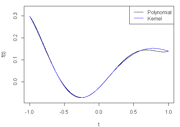
Figure 1: Plot showing $f_{1}$, $f_{2}$ constructed as described above. As one can see, the difference between the two functions is negligible.

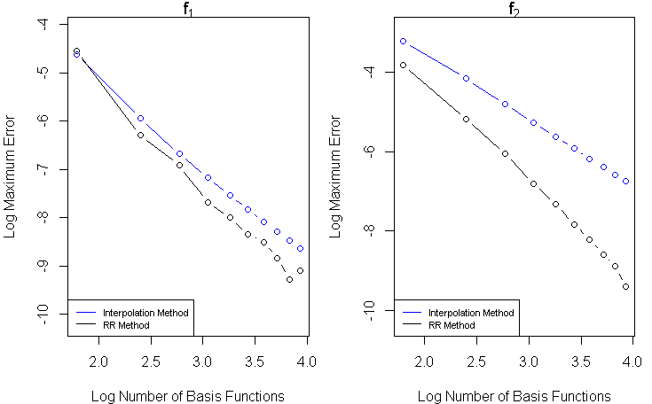
Figure 2: Plot showing the convergence rates of reproducing $f_{1}$ and $f_{2}$ via the RR method and the typical interpolation method seen in Gaussian process regression.

6.3 Numerical Examples

6.3.1 Boundary Conditions

As a basic application, let $T=[-1,1]^{2}$ and define $f$ by

$$f(t_{1},t_{2})=\frac{1}{2}e^{.2(t_{1}-.5)^{2}}\sin\Big{(}\frac{\pi t_{1}}{2}\Big{)}+e^{-x_{2}^{2}}\cos\Big{(}\frac{\pi x_{2}}{2}\Big{)}$$

Assume that the value of $f$ is known at $M$ points of the domain, as well as on

$$T_{0}=\partial T.$$

Since $T_{0}$ has dimension one, one may define a parameterization $\ell:[-1,1)\to T_{0}$ so that computations may be performed in one dimension. One practical issue with this however is that the function $f$ is continuously differentiable on $T$, whereas the function $f\circ\ell$ is not differentiable on $\{-1,-1/2,0,1/2\}$.

To assess the accuracy of the method for different numbers of basis functions, the test data used is a collection of points on the set $\mathcal{T}=\{(.9t,.9s):(t,s)\in\partial T\}$ and measure discrepancy based upon the the loss function

$$L(f,g)=\max_{t\in\mathcal{T}}|f(t)-g(t)|.$$

We select $M=10$, where the points on the interior are chosen via a Latin Hypercube sampling scheme. Figure 3 shows the error as the number of basis functions increases. Observe that the log error flattens out, unlike what is observed in Figure 2 from reproducing the function. This can be thought of as a phenomenon where essentially all of useful information from the boundary has been extracted, leading to diminishing returns on predictive power with additional basis functions.

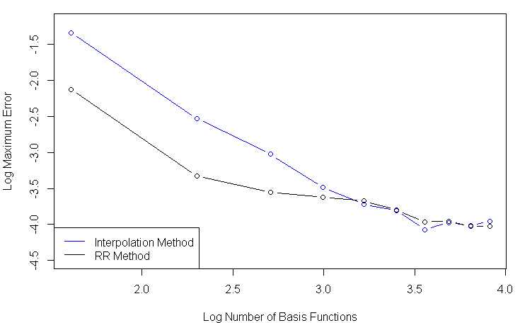
Figure 3: Plot of approximation error versus number of basis functions given boundary information, as described in Section 6.3.1.

6.3.2 Diagonal Conditions

As mentioned previously, $T_{0}$ is not limited to the boundary, and can be any subset of $T$. In this example, assume that $T=[-1,1]^{2}$, and let $T_{0}$ be the diagonal of $T$, i.e. $T_{0}=\{(t,t):t\in[-1,1]\}$. Define $f$ by

$$f(t_{1},t_{2})=t_{2}\sqrt{1+t_{1}}\cos(\pi t_{2})\sin\Big{(}\frac{\pi(t_{1}-t_{2})}{2}+1\Big{)}e^{.5(t_{1}+t_{2})^{2}}$$

Selecting $M=10$ as before, and choosing test points on the set $\mathcal{T}=T\cap\big{(}\{(t,t\pm.1):t\in[-1,1]\}\big{)}$, we again compute the maximum predictive error as a function of the number of basis functions for each method. Figure 4 suggests that all of the information from the diagonal is extracted very quickly using the RR method, whereas the convergence is much slower using the standard interpolation method to approximate the RKHS norm. This is likely due to the fact that a parameterization of the diagonal is differentiable whereas a parameterization of the boundary is not.

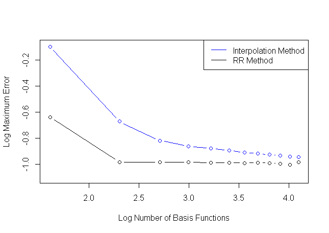
Figure 4: Plot of approximation error versus number of basis functions given information on the diagonal, as described in Section 6.3.2.

The results from these two examples indicate that our adopted approach in computing RKHS inner products has proven effective for incorporating information from more general subsets of the domain into a predictive Gaussian process model. Additionally, the method appears to be even more valuable in the case where the information available does not exist in the RKHS generated by the covariance kernel, which is certainly the case for the parameterized boundary in the first example, and likely the case in the complicated example given in the second example.

7 Conclusions and Future Directions

The goal of this paper was to construct Gaussian processes which are capable of using information from arbitrary connected subsets of the domain in a way which required minimal assumptions to be made. Using the theory of Reproducing Kernel Hilbert Spaces, we were able to explicitly define the conditional mean and covariance of Gaussian processes via orthogonal projections in an RKHS, prove that such processes exist, and show that the processes are optimal in the sense of minimizing pointwise mean square error given the initial assumptions made. In addition, we provided several numerical examples to exhibit the practical nature of our construction, which included evidence that one need not assume the functional information available is an element of a RKHS. Future work in this area includes extending the theory to more naturally handle the case where functional information is available on disjoint subsets of the domain. Another interesting avenue to extend this research is to provide a similar framework for including more general linear operator constraints, e.g. differential operator constraints.

References

- Arp et al. (Submitted) Joshua Arp, John Nicholson, Joseph Geddes, D. Brown, Sez Atamturktur, and Christopher Kitchens. Inferring effective interphase properties in composites by inverse analysis. ACS Applied Materials & Interfaces, Submitted.
- Berlinet and Thomas-Agnan (2004) Alain Berlinet and Christine Thomas-Agnan. Reproducing Kernel Hilbert Space in Probability and Statistics. 01 2004.
- Ha Quang (2010) Minh Ha Quang. Some properties of gaussian reproducing kernel hilbert spaces and their implications for function approximation and learning theory. Constructive Approximation, 32:307–338, 10 2010.
- Harari et al. (2017) Ofir Harari, A. Dean, D. Bingham, and D. Higdon. Computer experiments: Prediction accuracy, sample size and model complexity revisited. Statistica Sinica, 2017.
- Kallenberg (1997) Olav Kallenberg. Foundations of Modern Probability. Springer, 1997.
- Kennedy and O’Hagan (2001) Marc Kennedy and Anthony O’Hagan. Bayesian calibration of computer models. Journal of the Royal Statistical Society Series B, 63:425–464, 02 2001.
- Lange-Hegermann (2020) Markus Lange-Hegermann. Linearly constrained gaussian processes with boundary conditions. CoRR, 2020.
- Lax (2002) Peter Lax. Functional Analysis. Wiley, 2002.
- Loeppky et al. (2009) Jason Loeppky, Jerome Sacks, and William Welch. Choosing the sample size of a computer experiment: A practical guide. Technometrics, 51:366–376, 11 2009.
- Micchelli et al. (2006) Charles A. Micchelli, Yuesheng Xu, and Haizhang Zhang. Universal kernels. Journal of Machine Learning Research, 2006.
- Oya et al. (2009) Antonia Oya, Jesús Navarro-Moreno, and Juan Carlos Ruiz-Molina. Numerical evaluation of reproducing kernel hilbert space inner products. IEEE Transactions on Signal Processing, 57(3):1227–1233, 2009.
- Paulsen and Raghupathi (2016) V. I. Paulsen and M. Raghupathi. An Introduction to the Theory of Reproducing Kernel Hilbert Spaces. Cambridge University Press, 2016.
- Ranjan et al. (2011) Pritam Ranjan, Ronald Haynes, and Richard Karsten. A computationally stable approach to gaussian process interpolation of deterministic computer simulation data. Technometrics, 53(4):366–378, 2011.
- Rasmussen et al. (2006) C.E. Rasmussen, C.K.I. Williams, M.I.T. Press, F. Bach, and ProQuest (Firm). Gaussian Processes for Machine Learning. Adaptive computation and machine learning. MIT Press, 2006.
- Rudin (1991) W. Rudin. Functional Analysis. Higher mathematics series. McGraw-Hill, 1991.
- Solin and Särkkä (2019) Arno Solin and Simo Särkkä. Hilbert space methods for reduced-rank gaussian process regression. Statistics and Computing, 30:419–446, Aug 2019.
- Swiler et al. (2020) Laura P. Swiler, Mamikon Gulian, Ari L. Frankel, Cosmin Safta, and John D. Jakeman. A survey of constrained gaussian process regression: Approaches and implementation challenges. Journal of Machine Learning for Modeling and Computing, 1(2):119–156, 2020.
- Tan (2016) Matthias Tan. Gaussian process modeling with boundary information. Statistica Sinica, 10 2016.
- van der Vaart and van Zanten (2011) Aad van der Vaart and Harry van Zanten. Information rates of nonparametric gaussian process methods. Journal of Machine Learning Research, 12:2095–2119, 06 2011.