Schlömilch integrals and probability distributions on the simplex
David D. K. Chow

Abstract

The Schlömilch integral, a generalization of the Dirichlet integral on the simplex, and related probability distributions are reviewed. A distribution that unifies several generalizations of the Dirichlet distribution is presented, with special cases including the scaled Dirichlet distribution and certain Dirichlet mixture distributions. Moments and log-ratio covariances are found, where tractable. The normalization of the distribution motivates a definition, in terms of a simplex integral representation, of complete homogeneous symmetric polynomials of fractional degree.

1 Introduction

One of the most important multivariate integrals is the Dirichlet integral on the simplex [1], which is a multivariate generalization of the Euler beta function. Expressed as an integral over the simplex $S_{K}=\{\mathbf{y}=(y_{1},\ldots,y_{K})\subset\mathbb{R}^{K}:\sum_{i=1}^{K}y_{i}=1,y_{i}\geq 0\}$, the Dirichlet integral is

$$\int_{S_{K}}\textrm{d}^{K-1}y\,\!\prod_{i=1}^{K}y_{i}^{\alpha_{i}-1}=\frac{\prod_{i=1}^{K}\Gamma(\alpha_{i})}{\Gamma(\alpha_{+})},$$ (1.1)

where $\alpha_{i}>0$ and $\alpha_{+}=\sum_{i=1}^{K}\alpha_{i}$. Because of the sum constraint $\sum_{i=1}^{K}y_{i}=1$, we may regard the integrand as a function of $y_{1},\ldots,y_{K-1}$ and take

$$\int_{S_{K}}\textrm{d}^{K-1}y=\int_{0}^{1}\!\textrm{d}y_{1}\,\int_{0}^{1-y_{1}}\!\textrm{d}y_{2}\ldots\int_{0}^{1-y_{1}-\ldots-y_{K-2}}\!\textrm{d}y_{K-1}.$$ (1.2)

A generalization is the Schlömilch integral

$$\int_{S_{K}}\textrm{d}^{K-1}x\,\!\frac{\prod_{i=1}^{K}x_{i}^{\alpha_{i}-1}}{(\sum_{j=1}^{K}\beta_{j}x_{j})^{\alpha_{+}}}=\frac{\prod_{i=1}^{K}\Gamma(\alpha_{i})}{\Gamma(\alpha_{+})\prod_{i=1}^{K}\beta_{i}^{\alpha_{i}}},$$ (1.3)

where $\beta_{i}>0$, which was obtained by Schlömilch not long after the discovery of the Dirichlet integral, appearing first in the textbook [2] (p. 165), and then further developed in the article [3]. The Schlömilch integral (1.3) follows from the Dirichlet integral (1.1) through the coordinate transformation

$$y_{i}=\frac{\beta_{i}x_{i}}{\sum_{j=1}^{K}\beta_{j}x_{j}},$$ (1.4)

although it was originally derived in a more complicated manner. If all $\beta_{i}$ are equal, then this transformation is trivial and the Schlömilch integral (1.3) reduces to the Dirichlet integral (1.1).

Schlömilch gave a slightly more general result,

$$\int_{x_{i}\geq 0,\,\lambda\leq\sum_{i=1}^{K}x_{i}\leq\kappa}\!\textrm{d}^{K}x\,\frac{\prod_{i=1}^{K}x_{i}^{\alpha_{i}-1}}{(\theta+\sum_{j=1}^{K}\gamma_{j}x_{j})^{\alpha_{+}}}f({\textstyle\sum_{k=1}^{K}x_{k}})=\frac{\prod_{i=1}^{K}\Gamma(\alpha_{i})}{\Gamma(\alpha_{+})}\int_{\lambda}^{\kappa}\!\textrm{d}t\,\frac{t^{\alpha_{+}-1}f(t)}{\prod_{j=1}^{K}(\theta+\gamma_{j}t)^{\alpha_{j}}},$$ (1.5)

where $f$ is an arbitrary function, and we take $\beta_{i}=\theta+\gamma_{i}$ to facilitate comparison with the original literature. This type of generalization is analogous to Liouville’s well-known generalization of the Dirichlet integral. Taking $f(t)=\delta(t-1+\epsilon)$, i.e. a Dirac delta function centred at $1-\epsilon$ for some $\epsilon>0$, as well as $\lambda<1<\kappa$, then taking $\epsilon\rightarrow 0$, we obtain the Schlömilch integral (1.3). If all $\gamma_{i}$ are equal, then the more general Schlömilch integral (1.5) reduces to Liouville’s generalization of the Dirichlet integral.

The Schlömilch integral (1.3) or the slightly more general (1.5) have appeared in widely used textbooks from the late 19th and early 20th centuries, such as Todhunter (pp. 263–265 of [4]) and Edwards (pp. 169–173 of [5]). The result does not seem to have been widely used in research at that time, but an example is Dixon [6], who does not provide a reference, instead providing a self-contained derivation.

In contemporary use, the Schlömilch integral has applications in several areas of science and mathematics, and appears in reference books such as Gradshteyn and Ryzhik (entry 4.637 of [7]), Prudnikov, Brychkov and Marichev (Section 3.3.4 of [8]), and Zwillinger (p. 102 of [9]). The formula (1.3) is useful in both directions: it can be used directly as an evaluation of an integral on a simplex, but can also be used, as an intermediate step in a larger calculation, to replace $\prod_{i=1}^{K}\beta_{i}^{-\alpha_{i}}$ with a simplex integral. Perhaps most notably, the Schlömilch integral is in widespread use in quantum field theory, where it is a key tool for evaluating Feynman diagrams, with $x_{1},\ldots,x_{K-1}$ referred to as Feynman parameters, and the Schlömilch integral (1.3) sometimes attributed to Feynman. In this context, Feynman stated that the technique was suggested by Schwinger [10], as further explained in the historical study [11] (see in particular pp. 445 and 452–454). For a standard textbook treatment, see e.g. equation (6.42) of [12]; a recent review of Feynman integrals [13] considers Feynman parameters in Section 2.5.3. Despite its widespread use, the Schlömilch integral is not as well-known as it should be, as suggested by its rediscovery over the last few years in disparate fields [14, 15]; the Dirichlet integral itself has also been rederived recently [16]. Furthermore, the origin of the Schlömilch integral appears to have been completely forgotten.

Schlömilch pointed out that further results can be obtained by differentiating with respect to parameters. In equation (6) of [3], by differentiating with respect to $\theta$, is an equation equivalent to

$$\int_{\begin{subarray}{c}\\ \\ x_{i}\geq 0,\\ 0\leq\sum_{i=1}^{K}x_{i}\leq 1\end{subarray}}\!\textrm{d}^{K}x\,\frac{\prod_{i=1}^{K}x_{i}^{\alpha_{i}-1}f(\sum_{k=1}^{K}x_{k})}{(\theta+\sum_{j=1}^{K}\gamma_{j}x_{j})^{\alpha_{+}+1}}=\frac{\prod_{i=1}^{K}\Gamma(\alpha_{i})}{\Gamma(\alpha_{+}+1)}\int_{0}^{1}\!\textrm{d}t\,\frac{t^{\alpha_{+}-1}f(t)}{\prod_{j=1}^{K}(\theta+\gamma_{j}t)^{\alpha_{j}}}\sum_{i=1}^{K}\frac{\alpha_{i}}{\theta+\gamma_{i}t}.$$ (1.6)

Again by taking $f(t)=\delta(t-1+\epsilon)$ and then the limit $\epsilon\rightarrow 0$, we obtain the simplex integral

$$\int_{S_{K}}\textrm{d}^{K-1}x\,\!\frac{\prod_{i=1}^{K}x_{i}^{\alpha_{i}-1}}{(\sum_{j=1}^{K}\beta_{j}x_{j})^{\alpha_{+}+1}}=\frac{\prod_{i=1}^{K}\Gamma(\alpha_{i})}{\Gamma(\alpha_{+}+1)\prod_{j=1}^{K}\beta_{j}^{\alpha_{j}}}\sum_{i=1}^{K}\frac{\alpha_{i}}{\beta_{i}}.$$ (1.7)

This result may also be obtained by differentiating the Schlömilch integral (1.3) with respect to each $\beta_{i}$ and then summing. The differentiation procedure increases the exponent of the denominator of the integrand from $\alpha_{+}$ to $\alpha_{+}+1$ and can be repeated, increasing the exponent to $\alpha_{+}+n$, for positive integers $n$. In this article, we shall find explicit expressions for such integrals, and examine some further generalizations.

The Dirichlet integral and its generalizations have wide-ranging applications, but we shall focus here on applications to associated probability distributions on the simplex, for which these integrals appear in normalization constants. Through a special mixture distribution based on the Schlömilch integral, we shall provide a unified framework for several distributions appearing in the literature. Special cases include the G3D generalized Dirichlet distribution [17] or scaled Dirichlet distribution [18], the shifted-scaled Dirichlet distribution [19] or simplicial generalized beta distribution [20], the flexible Dirichlet distribution [21], and the tilted Dirichlet distribution [22]. In a similar manner, we shall also obtain a family of distributions that includes the Concrete or Gumbel-softmax distribution [23, 24]. By including additional parameters, these generalizations of the Dirichlet distribution allow for behaviours that the Dirichlet distribution itself cannot model, for example positive covariances $\textrm{Cov}(X_{i},X_{j})$.

Although we can show, through explicit computation, examples in which $\textrm{Cov}(X_{i},X_{j})$ is positive, moments cannot generally be computed so explicitly. Taking advantage of the fact that the distributions, when all parameters except $\boldsymbol{\alpha}$ are fixed, belong to the exponential family of distributions, it is easier to compute log-ratio covariances $\textrm{Cov}[\log(X_{i}/X_{j}),\log(X_{k}/X_{l})]$. Moreover, the importance of log-ratios has been emphasized in the context of compositional data analysis [18].

As a mathematical aside, the normalization constants of the distributions involve simplex integrals that relate to generalized hypergeometric functions, in particular the Carlson $R$-function, which is a rewriting of the Lauricella $F_{D}$-hypergeometric function. In certain cases these provide generalizations of the complete homogeneous symmetric polynomials $h_{n}(X_{1},\ldots,X_{K})$. Taking a converse viewpoint, we find a natural way of generalizing such polynomials from non-negative integer $n$ to fractional $n$ through an integral representation on the simplex $S_{K}$.

In Section 2, we review some known probability distributions on the simplex, unifying them within a common framework. Section 3 contains results of a more mathematical nature, for later use or to highlight connections to mathematical literature, in particular to symmetric polynomials. In Section 4, we examine properties of the distributions, deriving moments and log-ratio covariances. We conclude in Section 5.

2 Probability distributions

We first review some known probability distributions on the simplex and define our notation. The probability simplex is denoted $S_{K}$, where the subscript $K$ denotes the dimension of the embedding space $\mathbb{R}^{K}$; the simplex itself is $(K-1)$-dimensional. This can be a more natural notation for applications, so the sum constraint $\sum_{i=1}^{K}x_{i}=1$ corresponds to a unit interval being divided into $K$ parts.

For $K$-dimensional vectors, we use the notation $\boldsymbol{\alpha}=(\alpha_{1},\ldots,\alpha_{K})$ and denote the sum of components $\alpha_{+}=\sum_{i=1}^{K}\alpha_{i}$. The vectors that we consider have non-negative components, $\alpha_{i}\geq 0$, so $\alpha_{+}$ is also the $L^{1}$-norm of $\boldsymbol{\alpha}$, i.e. $\alpha_{+}=||\boldsymbol{\alpha}||_{1}$. $\mathbf{e}_{i}$ is a unit-vector in the $i$-direction, i.e. with $j$-component $(\mathbf{e}_{i})_{j}=\delta_{ij}$. The $K$-dimensional vector whose entries are all 1 is $\mathbf{1}=(1,\ldots,1)$. Given a vector $\boldsymbol{\beta}$, whose components are $\beta_{i}$, the vector $\boldsymbol{\beta}^{\sigma}$ is defined to have components $\beta_{i}^{\sigma}$, i.e. $\boldsymbol{\beta}^{\sigma}=(\beta_{1}^{\sigma},\ldots,\beta_{K}^{\sigma})$. We use bars to denote the operation of normalizing a vector to give a unit-vector, e.g. $\overline{\mathbf{1}}=\mathbf{1}/K$ and $\overline{\boldsymbol{\beta}^{-\sigma}}=\boldsymbol{\beta}^{-\sigma}/(\beta^{-\sigma})_{+}$.

2.1 Dirichlet, Schlömilch and generalized beta distributions

2.1.1 Dirichlet distribution

The $(K-1)$-variate Dirichlet distribution is parameterized by a $K$-dimensional vector $\boldsymbol{\alpha}=(\alpha_{1},\ldots,\alpha_{K})$, with $\alpha_{i}>0$. The probability density function, defined on the probability simplex $S_{K}$, is

$$f(\mathbf{x})=\frac{\Gamma(\alpha_{+})}{\prod_{i=1}^{K}\Gamma(\alpha_{i})}\prod_{i=1}^{K}x_{i}^{\alpha_{i}-1}.$$ (2.1)

The Dirichlet integral (1.1) ensures the normalization $\int_{S_{K}}\!\textrm{d}^{K-1}x\,f(\mathbf{x})=1$, which is why Wilks gave the Dirichlet distribution its name [25]. For a random variable $\mathbf{Y}=(Y_{1},\ldots,Y_{K})$ with this Dirichlet distribution, we denote $\mathbf{Y}\sim D(\boldsymbol{\alpha})$. The special case $D(\mathbf{1})$ is simply a uniform distribution on the simplex. Samples from the Dirichlet distribution $\mathbf{Y}$ can be generated from samples of standard gamma distributions $Z_{i}$ through

$$Y_{i}=\frac{Z_{i}}{\sum_{j=1}^{K}Z_{j}},$$ (2.2)

where $Z_{i}\sim\textrm{Gamma}(\alpha_{i},1)$ and $\alpha_{i}$ are shape parameters.

The mean, variance, and covariance for $i\neq j$ are

$$\mathbb{E}(Y_{i}) =\frac{\alpha_{i}}{\alpha_{+}}, \textrm{Var}(Y_{i}) =\frac{\alpha_{i}(\alpha_{+}-\alpha_{i})}{\alpha_{+}^{2}(\alpha_{+}+1)}, \textrm{Cov}(Y_{i},Y_{j})=-\frac{\alpha_{i}\alpha_{j}}{\alpha_{+}^{2}(\alpha_{+}+1)}.$$ (2.3)

The $K$ independent parameters of $\boldsymbol{\alpha}$ can be considered as corresponding to $K-1$ independent means and an overall scaling of the covariance. Note that $\textrm{Cov}(Y_{i},Y_{j})$ is always negative, so the distribution is not appropriate for modelling data that has negative covariances.

For background on the Dirichlet distribution, including basic properties, applications and generalizations, see e.g. [25, 26, 27]; a review of its history is [28].

2.1.2 Schlömilch distribution

A more general family of distributions defined on $S_{K}$ is given by the probability density function

$$f(\mathbf{x})=\frac{\Gamma(\alpha_{+})\prod_{j=1}^{K}\beta_{j}^{\alpha_{j}}}{\prod_{i=1}^{K}\Gamma(\alpha_{i})}\frac{\prod_{i=1}^{K}x_{i}^{\alpha_{i}-1}}{(\sum_{j=1}^{K}\beta_{j}x_{j})^{\alpha_{+}}}.$$ (2.4)

Compared to the Dirichlet distribution, there are double the number of parameters, with an additional $K$-dimensional parameter vector $\boldsymbol{\beta}=(\beta_{1},\ldots,\beta_{K})$, with $\beta_{i}>0$. The distribution is invariant under rescaling $\boldsymbol{\beta}\rightarrow\lambda\boldsymbol{\beta}$, for $\lambda>0$, so there are $2K-1$ independent parameters. For identifiability when performing statistical inference, we may assume that $\sum_{i=1}^{K}\beta_{i}=1$, which implies that $\beta_{i}<1$. If all $\beta_{i}$ are equal, then the Dirichlet distribution is recovered.

In statistical literature, the distribution (2.4) seems to have first appeared in work of Dickey [29], obtained from the Dirichlet distribution through the transformation (1.4) and attributed to a Savage communication. Some other early appearances include the generalized Dirichlet distribution (G3D) of Chen and Novick [17] and the scaled Dirichlet distribution of Aitchison [18]. A more recent appearance is the gamma normalized infinitely divisible (NID) distribution [30, 31], although one should note that the generalized gamma distribution, from which it is derived, is infinitely divisible for only certain ranges of its parameters.

A further parameter $\tau>0$ may be introduced, giving a distribution with probability density function

$$f(\mathbf{x})=\frac{\tau^{K-1}\Gamma(\alpha_{+})}{(\sum_{j=1}^{K}\beta_{j}x_{j}^{\tau})^{\alpha_{+}}}\prod_{i=1}^{K}\frac{\beta_{i}^{\alpha_{i}}x_{i}^{\tau\alpha_{i}-1}}{\Gamma(\alpha_{i})}.$$ (2.5)

This distribution was obtained by Craiu and Craiu [32] (see also Chapter 49.1 of [26]), by transformation of generalized gamma distributions. Equivalently, the transformation can be expressed in terms of standard gamma distributions as

$$X_{i}=\frac{(Z_{i}/\beta_{i})^{1/\tau}}{\sum_{j=1}^{K}(Z_{j}/\beta_{j})^{1/\tau}},$$ (2.6)

where $Z_{i}\sim\textrm{Gamma}(\alpha_{i},1)$ and $\alpha_{i}$ are shape parameters.

The case $\tau=1$ corresponds to the coordinate transformation (1.4) and the distribution (2.4). The distribution (2.5) has also been called the shifted-scaled Dirichlet distribution [19] and the simplicial generalized beta distribution [20]. The special case with $\boldsymbol{\beta}=\overline{\mathbf{1}}$ has also been called the generalized Dirichlet distribution [33].

For the probability density function (2.5), we shall denote the corresponding distribution by $S(\boldsymbol{\alpha},\boldsymbol{\beta},\tau)$. The $S$ stands for Schlömilch, Savage, scaled, shifted, or simplicial, according to taste. I shall refer to the $S$-distribution as the Schlömilch distribution, in order to complement the distribution named after Dirichlet.

Recalling the expression (2.2), which relates a Dirichlet random variable to gamma random variables, we see that there is a transformation relating a Dirichlet random variable $\mathbf{Y}\sim D(\boldsymbol{\alpha})$ and a Schlömilch random variable $\mathbf{X}\sim S(\boldsymbol{\alpha},\boldsymbol{\beta},\tau)$,

$$Y_{i} =\frac{\beta_{i}X_{i}^{\tau}}{\sum_{j=1}^{K}\beta_{j}X_{k}^{\tau}}, X_{i} =\frac{(Y_{i}/\beta_{i})^{1/\tau}}{\sum_{j=1}^{K}(Y_{j}/\beta_{j})^{1/\tau}}.$$ (2.7)

In general, this transformation is trivial if and only if both $\tau=1$ and all $\beta_{i}$ are equal.

2.1.3 Univariate distributions: generalized beta

In the univariate case, $K=2$, the Dirichlet distribution is simply the beta distribution. The three-parameter generalized beta distribution (G3B) of Libby and Novick [34] matches the univariate Schlömilch distribution with $\tau=1$, i.e. (2.4); later rediscoveries include [35, 36, 37].

More generally, the four-parameter generalized beta distribution (G4B) of Chen and Novick [17] has probability density function of the form

$$f(x)=\frac{\Gamma(\alpha_{1}+\alpha_{2})}{\Gamma(\alpha_{1})\Gamma(\alpha_{2}){{}_{2}}F{{}_{1}}(\alpha_{1},\kappa;\alpha_{+};1-\lambda)}\frac{x^{\alpha_{1}-1}(1-x)^{\alpha_{2}-1}}{(\lambda x+1-x)^{\kappa}},$$ (2.8)

where $\alpha_{i}>0$, $\kappa>0$ and $\lambda>0$. Choosing $\kappa=\alpha_{1}+\alpha_{2}$ recovers the G3B distribution. The hypergeometric function ${{}_{2}}F{{}_{1}}(\alpha_{1},\kappa;\alpha_{+};1-\lambda)$ can be defined by demanding the normalization condition $\int_{0}^{1}\!\textrm{d}x\,f(x)=1$; this corresponds to the Euler integral representation

$${{}_{2}}F{{}_{1}}(a,b;c;x)=\frac{\Gamma(c)}{\Gamma(b)\Gamma(c-b)}\int_{0}^{1}\!\textrm{d}t\,t^{b-1}(1-t)^{c-b-1}(1-xt)^{-a},$$ (2.9)

defined for $\textrm{Re}\,c>\textrm{Re}\,b>0$ and then analytically continued. Other early appearances of the distribution include the hypergeometric family of Chamayou and Letac [38], and the Gauss hypergeometric distribution of Armero and Bayeri [39].

In the case that $\kappa=\alpha_{+}+n$, for a non-negative integer $n$, the G4B distribution is a finite mixture of Schlömilch distributions. To see this, multiply the probability density function (2.8) by $1=(x+1-x)^{n}$ and use a binomial expansion, giving

$$f(x)=\sum_{k=0}^{n}w_{k}f_{k}(x),$$ (2.10)

where the weights are

$$w_{k}=\binom{n}{k}\frac{(\alpha_{1})_{k}(\alpha_{2})_{n-k}}{(\alpha_{+})_{n}\lambda^{\alpha_{1}+k}{{}_{2}}F{{}_{1}}(\alpha_{1},\alpha_{+}+n;\alpha_{+};1-\lambda)},$$ (2.11)

the Pochhammer symbol denotes the rising factorial, i.e. $(x)_{n}=x(x+1)\ldots(x+n-1)$, and

$$f_{k}(x)=\frac{\Gamma(\alpha_{+}+n)\lambda^{\alpha_{1}+k}}{\Gamma(\alpha_{1}+k)\Gamma(\alpha_{2}+n-k)}\frac{x^{\alpha_{1}+k-1}(1-x)^{\alpha_{2}+n-k-1}}{(\lambda x+1-x)^{\alpha_{+}+n}}$$ (2.12)

is the probability density function of an $S(\alpha_{1}+k,\alpha_{2}+n-k,\frac{\lambda}{\lambda+1},\frac{1}{\lambda+1},1)$ distribution.

Note that, because $\sum_{k=0}^{n}w_{k}=1$, the hypergeometric function can be expressed as a finite sum as

$${{}_{2}}F{{}_{1}}(\alpha_{1},\alpha_{+}+n;\alpha_{+};1-\lambda)=\sum_{k=0}^{n}\binom{n}{k}\frac{(\alpha_{1})_{k}(\alpha_{2})_{n-k}}{(\alpha_{+})_{n}\lambda^{\alpha_{1}+k}}.$$ (2.13)

This is equivalent to a known relation for the hypergeometric function,

$${{}_{2}}F{{}_{1}}(\alpha_{1},\alpha_{+}+n;\alpha_{+};1-\lambda)=\frac{(\alpha_{2})_{n}\,{{}_{2}}F{{}_{1}}(\alpha_{1},-n;1-n-\alpha_{2};\lambda^{-1})}{(\alpha_{+})_{n}\lambda^{\alpha_{1}}},$$ (2.14)

by using the definition of the hypergeometric function on the right as a power series that converges for $|\lambda^{-1}|<1$, analytically continued. Although a known result, I have been unable to find a direct derivation in easily accessible literature. It may be derived from known properties of the hypergeometric function, using the Euler transformation

$${{}_{2}}F{{}_{1}}(a,b;c;x)=(1-x)^{c-a-b}{{}_{2}}F{{}_{1}}(c-a,c-b;c;x),$$ (2.15)

and taking the $a\rightarrow-n$ limit, with $b=\alpha_{2}$, $c=\alpha_{1}+\alpha_{2}$ and $x=1-\lambda$, in the relation (see e.g. Chapter 1.8 of [40])

$${{}_{2}}F{{}_{1}}(a,b;c;x) =\frac{\Gamma(b-a)\Gamma(c)}{\Gamma(b)\Gamma(c-a)}(1-x)^{-a}{{}_{2}}F{{}_{1}}(a,c-b;a-b+1;1/(1-x))$$

$$\qquad+\frac{\Gamma(a-b)\Gamma(c)}{\Gamma(a)\Gamma(c-b)}(1-x)^{-b}{{}_{2}}F{{}_{1}}(b,c-a;b-a+1;1/(1-x)),$$ (2.16)

which is a linear relation between three of Kummer’s 24 solutions of the hypergeometric equation, a linear, second-order differential equation.

A different generalization of the G3B distribution is given by the $GB(a,b,c,\alpha_{1},\alpha_{2})$ distribution of McDonald and Xu [41], which has support on $(0,b/(1-c)^{1/a})$, where $b>0$ and $0\leq c\leq 1$. Choosing $a>0$ and $b=(1-c)^{1/a}$, with $c\neq 1$, we have a 4-parameter family of distributions with support on $(0,1)$, with probability density function

$$f(x)=\frac{\Gamma(\alpha_{1}+\alpha_{2})ax^{a\alpha_{1}-1}(1-x^{a})^{\alpha_{2}-1}}{\Gamma(\alpha_{1})\Gamma(\alpha_{2})(1-c)^{\alpha_{1}}[1+cx^{a}/(1-c)]^{\alpha_{1}+\alpha_{2}}}.$$ (2.17)

This is the univariate case, $K=2$, of the Schlömilch distribution (2.5). The case $a=1$ reduces to the G3B distribution.

2.2 Mixture distributions

2.2.1 Normalization constant for Dirichlet mixture

Consider a special Dirichlet mixture distribution, which we denote $DM(\boldsymbol{\alpha},\boldsymbol{\gamma},n,\sigma)$, with probability density function of the form

$$f(\mathbf{x})=\frac{1}{I_{n}^{\sigma}(\boldsymbol{\alpha},\boldsymbol{\gamma})}\bigg{(}\sum_{k=1}^{K}\gamma_{k}x_{k}^{\sigma}\bigg{)}^{n}\prod_{i=1}^{K}x_{i}^{\alpha_{i}-1},$$ (2.18)

where $n$ is a positive integer, $\sigma>0$ and, for identifiability, we restrict the parameter vector $\boldsymbol{\gamma}$ to have unit-norm, i.e. $\gamma_{+}=1$. We define the function

$$I_{n}^{\sigma}(\boldsymbol{\alpha},\boldsymbol{\gamma})=\int_{S_{K}}\!\textrm{d}^{K-1}y\,\bigg{(}\sum_{k=1}^{K}\gamma_{k}y_{k}^{\sigma}\bigg{)}^{n}\prod_{i=1}^{K}y_{i}^{\alpha_{i}-1},$$ (2.19)

where the arguments satisfy $\alpha_{i}>0$, $\gamma_{i}>0$, $\sigma>0$, which plays the role of a normalization constant for the Dirichlet mixture distribution. For most of our study, it suffices to take $n$ to be a non-negative integer, although the function can be extended to real $n$ and, with a choice of branch cut, to complex $n$. The function $I_{n}^{\sigma}(\boldsymbol{\alpha},\boldsymbol{\gamma})$ satisfies the scaling $I_{n}^{\sigma}(\boldsymbol{\alpha},\lambda\boldsymbol{\gamma})=\lambda^{n}I_{n}^{\sigma}(\boldsymbol{\alpha},\boldsymbol{\gamma})$, for $\lambda>0$, implying that $I_{n}^{\sigma}(\boldsymbol{\alpha},\boldsymbol{\gamma})=\gamma_{+}^{n}I_{n}^{\sigma}(\boldsymbol{\alpha},\overline{\boldsymbol{\gamma}})$.

The Dirichlet mixture distribution $DM(\boldsymbol{\alpha},\boldsymbol{\gamma},n,\sigma)$ can be explicitly expressed as a mixture of Dirichlet distributions by decomposing its probability density function (2.18) as

$$f(\mathbf{x})=\sum_{n_{+}=n}w_{\mathbf{n}}f_{\mathbf{n}}(\mathbf{x}),$$ (2.20)

where $f_{\mathbf{n}}(\mathbf{x})$ is the probability density function of a Dirichlet distribution $D(\boldsymbol{\alpha}+\sigma\mathbf{n})$ obtained from (2.1). The summation is over non-negative integers $n_{1},\ldots,n_{K}$ such that $\sum_{i=1}^{K}n_{i}=n$. The weights are

$$w_{\mathbf{n}}=\frac{1}{I_{n}^{\sigma}(\boldsymbol{\alpha},\boldsymbol{\gamma})\Gamma(\alpha_{+}+\sigma n)}\binom{n}{\mathbf{n}}\prod_{i=1}^{K}\Gamma(\alpha_{i}+\sigma n_{i})\gamma_{i}^{n_{i}},$$ (2.21)

using the notation for a multinomial coefficient

$$\binom{n}{\mathbf{m}}=\frac{n!}{\prod_{i=1}^{K}m_{i}!},$$ (2.22)

where $\sum_{i=1}^{K}m_{i}=n$. The overall normalization of the Dirichlet mixture distribution implies that $\sum_{\mathbf{n}}w_{\mathbf{n}}=1$, and so we deduce an expression for $I_{n}^{\sigma}(\boldsymbol{\alpha},\boldsymbol{\gamma})$ as a finite sum,

$$I_{n}^{\sigma}(\boldsymbol{\alpha},\boldsymbol{\gamma})=\frac{1}{\Gamma(\alpha_{+}+\sigma n)}\sum_{n_{+}=n}\binom{n}{\mathbf{n}}\prod_{i=1}^{K}\Gamma(\alpha_{i}+\sigma n_{i})\gamma_{i}^{n_{i}},$$ (2.23)

which relies on $n$ being a non-negative integer. In some cases, which we consider later, this sum may be further simplified.

2.2.2 Jacobian computation

We perform a coordinate change from $\mathbf{y}$ to $\mathbf{x}$ coordinates by defining

$$x_{i}=\frac{(y_{i}/\beta_{i})^{1/\tau}}{\sum_{j=1}^{K}(y_{j}/\beta_{j})^{1/\tau}},$$ (2.24)

for $\tau>0$, corresponding to the transformation of random variables (2.7). It is clear that $\sum_{i=1}^{K}x_{i}=1$, so $\mathbf{x}$ are coordinates on the simplex $S_{K}$. The inverse coordinate transformation is

$$y_{i}=\frac{\beta_{i}x_{i}^{\tau}}{\sum_{j=1}^{K}\beta_{j}x_{j}^{\tau}}.$$ (2.25)

By computing the Jacobian, we obtain the transformation of the measure

$$\frac{\textrm{d}^{K-1}y}{\prod_{i=1}^{K}y_{i}}=\tau^{K-1}\frac{\textrm{d}^{K-1}x}{\prod_{i=1}^{K}x_{i}}.$$ (2.26)

It is a routine calculation to use the explicit coordinate transformations of (2.24) or (2.25) and compute partial derivatives $\partial y_{i}/\partial x_{j}$ or $\partial x_{i}/\partial y_{j}$ to find the Jacobian. However, a more implicit expression of the coordinate change gives a clearer understanding of the origin of the transformation of the measure (2.26). From (2.24) or (2.25), we have the differential relation

$$\textrm{d}\log\bigg{(}\frac{y_{i}}{y_{K-1}}\bigg{)}=\tau\,\textrm{d}\log\bigg{(}\frac{x_{i}}{x_{K-1}}\bigg{)}.$$ (2.27)

Remembering that $y_{K}$ is expressed in terms of the independent coordinates as $y_{K}=1-\sum_{i=1}^{K-1}y_{i}$, we take exterior products to compute the volume form (Chapter 2 of [42] provides an introduction to differential forms in a statistical context)

$$\textrm{d}\log\bigg{(}\frac{y_{1}}{y_{K-1}}\bigg{)}\wedge\textrm{d}\log\bigg{(}\frac{y_{2}}{y_{K-1}}\bigg{)}\wedge\ldots\wedge\textrm{d}\log\bigg{(}\frac{y_{K-2}}{y_{K-1}}\bigg{)}\wedge\textrm{d}\log\bigg{(}\frac{y_{K}}{y_{K-1}}\bigg{)}$$

$$=\bigg{(}\frac{\textrm{d}y_{1}}{y_{1}}-\frac{\textrm{d}y_{K-1}}{y_{K-1}}\bigg{)}\wedge\bigg{(}\frac{\textrm{d}y_{2}}{y_{2}}-\frac{\textrm{d}y_{K-1}}{y_{K-1}}\bigg{)}\wedge\ldots\wedge\bigg{(}\frac{\textrm{d}y_{K-2}}{y_{K-2}}-\frac{\textrm{d}y_{K-1}}{y_{K-1}}\bigg{)}\wedge\bigg{(}-\sum_{i=1}^{K-1}\frac{\textrm{d}y_{i}}{y_{K}}-\frac{\textrm{d}y_{K-1}}{y_{K-1}}\bigg{)}$$

$$=\frac{\textrm{d}y_{1}\wedge\textrm{d}y_{2}\wedge\ldots\wedge\textrm{d}y_{K-1}}{\prod_{i=1}^{K-1}y_{i}}\bigg{(}-1-\frac{\sum_{i=1}^{K-1}y_{i}}{y_{K}}\bigg{)}$$

$$=-\frac{\textrm{d}y_{1}\wedge\textrm{d}y_{2}\wedge\ldots\wedge\textrm{d}y_{K-1}}{\prod_{i=1}^{K}y_{i}}.$$ (2.28)

From the same calculation with $\mathbf{x}$ instead of $\mathbf{y}$, and the differential relation (2.27), we obtain

$$\frac{\textrm{d}y_{1}\wedge\textrm{d}y_{2}\wedge\ldots\wedge\textrm{d}y_{K-1}}{\prod_{i=1}^{K}y_{i}}=\tau^{K-1}\frac{\textrm{d}x_{1}\wedge\textrm{d}x_{2}\wedge\ldots\wedge\textrm{d}x_{K-1}}{\prod_{i=1}^{K}x_{i}},$$ (2.29)

which is the transformation of the measure (2.26) equivalently expressed in terms of volume forms.

Note that the computation works in the same way for the opposite sign of $\tau$, by replacing $\tau\rightarrow-\tau$, giving an extra factor of $(-1)^{K-1}$. When computing an integral over the simplex, this factor is cancelled out by consistently ordering the limits of the integral.

2.2.3 Schlömilch mixture distribution

The coordinate transformation leads to the special Schlömilch mixture distribution, which we denote by

$$\mathbf{X}\sim SM(\boldsymbol{\alpha},\boldsymbol{\beta},\boldsymbol{\gamma},n,\sigma,\tau).$$ (2.30)

Using the transformation of the measure given by (2.26), we obtain the probability density function

$$f(\mathbf{x})=\frac{\tau^{K-1}(\prod_{l=1}^{K}\beta_{l}^{\alpha_{l}})(\sum_{k=1}^{K}\beta_{k}^{\sigma}\gamma_{k}x_{k}^{\sigma\tau})^{n}\prod_{i=1}^{K}x_{i}^{\tau\alpha_{i}-1}}{I_{n}^{\sigma}(\boldsymbol{\alpha},\boldsymbol{\gamma})(\sum_{j=1}^{K}\beta_{j}x_{j}^{\tau})^{\alpha_{+}+\sigma n}},$$ (2.31)

where $n$ is a positive integer, $\sigma>0$, $\tau>0$. For identifiability, we restrict the parameter vectors $\boldsymbol{\beta}$ and $\boldsymbol{\gamma}$ to have unit-norm, i.e. $\beta_{+}=\gamma_{+}=1$, so there are $3K$ independent continuous parameters, in addition to the non-negative integer parameter $n$.

The Schlömilch mixture distribution can be explicitly expressed as a mixture of Schlömilch distributions by decomposing its probability density function (2.31) as

$$f(\mathbf{x})=\sum_{n_{+}=n}w_{\mathbf{n}}f_{\mathbf{n}}(\mathbf{x}),$$ (2.32)

where $f_{\mathbf{n}}(\mathbf{x})$ is the probability density function of a Schlömilch distribution $S(\boldsymbol{\alpha}+\sigma\mathbf{n},\boldsymbol{\beta},\tau)$ obtained from (2.4). The weights $w_{\mathbf{n}}$ are (2.21), the same as for the original Dirichlet mixture distribution.

2.2.4 Relations between distributions

The connections between the four key families of distributions are illustrated in Figure 1. To generate samples from the Schlömilch mixture distribution, one can generate samples from the Dirichlet distribution, followed by taking mixtures and transforming.

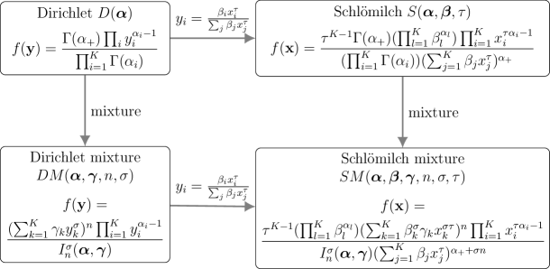
Figure 1: Two routes from the Dirichlet distribution to the Schlömilch mixture distribution

Conversely, one may regard the Schlömilch mixture distribution as providing a unified framework for several distributions that correspond to special choices of parameters, as seen from the probability density functions in Figure 1, remembering the constraint $\sum_{i=1}^{K}x_{i}=1$. For each positive integer $n$, the Schlömilch mixture distribution $SM(\boldsymbol{\alpha},\boldsymbol{\beta},\boldsymbol{\gamma},n,\sigma,\tau)$ contains, as special cases, the Dirichlet mixture distribution $DM(\boldsymbol{\alpha},\boldsymbol{\gamma},n,\sigma)$, the Schlömilch distribution $S(\boldsymbol{\alpha},\boldsymbol{\beta},\tau)$ and the Dirichlet distribution $D(\boldsymbol{\alpha})$.

More generally, there are three special cases in which the probability density function of the Schlömilch mixture distribution (2.31) simplifies. The first case is when the denominator factor $\sum_{j=1}^{K}\beta_{j}x_{j}^{\tau}$ is constant, corresponding to the Dirichlet mixture distribution. The second case is when the numerator factor $\sum_{k=1}^{K}\beta_{k}^{\sigma}\gamma_{k}x_{k}^{\sigma\tau}$ and the denominator factor $\sum_{j=1}^{K}\beta_{j}x_{j}^{\tau}$ are proportional, leaving only the denominator factor with a reduced exponent, which is the Schlömilch distribution. The third case is when the numerator factor $\sum_{j=1}^{K}\beta_{j}^{\sigma}\gamma_{j}x_{j}^{\sigma\tau}$ is constant, by taking $\gamma_{i}=\beta_{i}^{-\sigma}/(\beta^{-\sigma})_{+}$ and $\sigma\tau=1$, giving the probability density function

$$f(\mathbf{x})=\frac{(\prod_{l=1}^{K}\beta_{l}^{\alpha_{l}})\prod_{i=1}^{K}x_{i}^{\alpha_{i}/\sigma-1}}{\sigma^{K-1}I_{n}^{\sigma}(\boldsymbol{\alpha},\boldsymbol{\beta}^{-\sigma})(\sum_{j=1}^{K}\beta_{j}x_{j}^{1/\sigma})^{\alpha_{+}+\sigma n}}.$$ (2.33)

In the univariate $K=2$ case with $\sigma=1$ and $n$ generalized to take continuous values, this corresponds to the G4B distribution of (2.8).

The most basic $n=1$ case illustrates how the Dirichlet, Dirichlet mixture and Schlömilch distributions arise as special cases of the Schlömilch mixture distribution, as shown in Figure 2. In this $n=1$ case, the Dirichlet mixture distribution, which is a general mixture of $D(\boldsymbol{\alpha}+\sigma\mathbf{e}_{i})$ distributions, has been called the flexible Dirichlet distribution by Ongaro, Migliorati and Monti [21] ([27] prefers to call it the mixed Dirichlet distribution). The flexible Dirichlet distribution has been further studied in [43, 44] and, unlike the Dirichlet distribution, allows for multi-modality. Figure 2 explicitly includes the uniform distribution $D(\mathbf{1})$ and the scaled Dirichlet or G3D distribution, as discussed in Section 2.1.2, which arise as special cases of the Schlömilch mixture distribution for any choice of $n$.

In addition, Figure 2 includes $SM(\boldsymbol{\alpha},\overline{\boldsymbol{\alpha}},\overline{\boldsymbol{\alpha}^{-1}},1,1,1)$, i.e. (2.33) with $\boldsymbol{\beta}=\overline{\boldsymbol{\alpha}}$, $n=1$ and $\tau=1$, for which $\mathbb{E}X_{i}=1/K$ (so $\mathbb{E}\sum_{i=1}^{K}X_{i}=1$). This distribution has been used in the context of multivariate extreme value theory by Coles and Tawn [22], and has subsequently been referred to as the tilted Dirichlet distribution. The normalization involves $I_{1}^{1}(\boldsymbol{\alpha},\boldsymbol{\alpha}^{-1})=K\prod_{i=1}^{K}\Gamma(\alpha_{i})/\Gamma(1+\alpha_{+})$, as known to Schlömilch in (1.7), and so the probability density function is

$$f(\mathbf{x})=\frac{\Gamma(1+\alpha_{+})}{K}\bigg{(}\prod_{l=1}^{K}\frac{\alpha_{l}^{\alpha_{l}}}{\Gamma(\alpha_{l})}\bigg{)}\frac{\prod_{i=1}^{K}x_{i}^{\alpha_{i}-1}}{(\sum_{j=1}^{K}\alpha_{j}x_{j})^{\alpha_{+}+1}}.$$ (2.34)

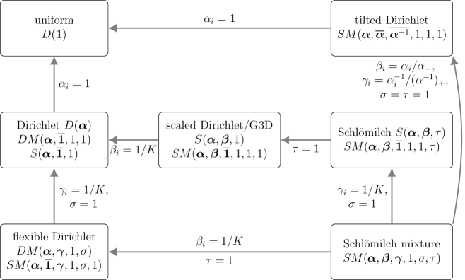
Figure 2: Relations between $n=1$ distributions

The $n=2$ case has received less attention in the literature. However, the recently considered double flexible Dirichlet distribution [45] is a general mixture of $D(\boldsymbol{\alpha}+\sigma(\mathbf{e}_{i}+\mathbf{e}_{j}))$ distributions, involving $\binom{K}{2}-1$ independent mixture weights. This includes the more restricted $DM(\boldsymbol{\alpha},\boldsymbol{\gamma},2,\sigma)$ distribution, which involves only $K-1$ independent mixture weights.

2.3 Inverse Schlömilch distribution

Consider the distribution constructed by taking

$$X_{i}=\frac{(\beta_{i}/Z_{i})^{1/\tau}}{\sum_{j=1}^{K}(\beta_{j}/Z_{j})^{1/\tau}},$$ (2.35)

where $Z_{i}\sim\textrm{Gamma}(\alpha_{i},1)$ and $\alpha_{i}$ are shape parameters. Again, the components of $\boldsymbol{\beta}$ are positive, $\beta_{i}>0$, and we shall assume that $\sum_{i=1}^{K}\beta_{i}=1$ for identifiability. This is simply the transformation used previously in (2.6), with the replacement $\tau\rightarrow-\tau$; however, it is convenient to state this transformation separately, continuing to take $\tau>0$, for comparison with literature. Using the transformation of the measure given by (2.26), but with $\tau\rightarrow-\tau$, we obtain the probability density function

$$f(\mathbf{x})=\frac{\tau^{K-1}\Gamma(\alpha_{+})}{(\sum_{j=1}^{K}\beta_{j}/x_{j}^{\tau})^{\alpha_{+}}}\prod_{i=1}^{K}\frac{\beta_{i}^{\alpha_{i}}}{\Gamma(\alpha_{i})x_{i}^{\tau\alpha_{i}+1}}.$$ (2.36)

We shall call this an inverse Schlömilch distribution $IS(\boldsymbol{\alpha},\boldsymbol{\beta},\tau)$.

The special case $IS(\mathbf{1},\boldsymbol{\beta},\tau)$ has applications in neural networks, where it has been called the Concrete distribution [23] (“Concrete” is a portmanteau of “continuous” and “discrete”) and the Gumbel-softmax distribution [24]. If $\alpha_{i}=1$, then $Z_{i}\sim\textrm{Exponential}(1)$ is a unit exponential distribution and $W_{i}=-\log Z_{i}\sim\textrm{Gumbel}(0,1)$ is a standard Gumbel distribution. Then the transformation (2.35) takes the form

$$X_{i}=\textrm{softmax}[(\mathbf{W}+\log\boldsymbol{\beta})/\tau]_{i},$$ (2.37)

where $\log\boldsymbol{\beta}=(\log\beta_{1},\ldots,\log\beta_{K})$ and the softmax function, given by

$$\textrm{softmax}(\mathbf{x})_{i}=\frac{\exp(x_{i})}{\sum_{j=1}^{K}\exp(x_{j})},$$ (2.38)

is a mapping from $\mathbb{R}^{K}$ to $S_{K}\subset\mathbb{R}^{K}$. In this context, the parameter $\tau$ is called a temperature, and the $\tau\rightarrow 0$ limit tends to a categorical distribution. The vector $\boldsymbol{\beta}$ is related to the corresponding probabilities of a categorical distribution; the constraint $\sum_{i=1}^{K}\beta_{i}=1$ ensures that they are normalized as probabilities. The more general inverse Schlömilch distribution $IS(\boldsymbol{\alpha},\boldsymbol{\beta},\tau)$ may therefore be considered as a Dirichlet–Concrete or Dirichet–Gumbel-softmax distribution.

The special case $IS(\boldsymbol{\alpha},\boldsymbol{\beta},1)$ has been considered by del Castillo [46], through the same construction but expressed in terms of chi-squared distributions instead of gamma distributions. Within the del Castillo distribution, the case $IS(\tfrac{1}{2}\mathbf{1},\boldsymbol{\beta},1)$ is an example from the ratio-stable distributions considered by Carlton [47, 48], parameterized by $\boldsymbol{\beta}$ and one extra parameter, which are related to a Dirichlet process.

In the univariate $K=2$ case, the inverse Schlömilch distribution $IS(\boldsymbol{\alpha},\boldsymbol{\beta},\tau)$ has probability density function

$$f(x) =\frac{\tau\Gamma(\alpha_{1}+\alpha_{2})\beta_{1}^{\alpha_{1}}\beta_{2}^{\alpha_{2}}}{\Gamma(\alpha_{1})\Gamma(\alpha_{2})x^{\tau\alpha_{1}+1}(1-x)^{\tau\alpha_{2}+1}[\beta_{1}/x^{\tau}+\beta_{2}/(1-x)^{\tau}]^{\alpha_{+}}}$$

$$=\frac{\tau\Gamma(\alpha_{1}+\alpha_{2})\beta_{1}^{\alpha_{1}}\beta_{2}^{\alpha_{2}}x^{\tau\alpha_{2}-1}(1-x)^{\tau\alpha_{1}-1}}{\Gamma(\alpha_{1})\Gamma(\alpha_{2})[\beta_{2}x^{\tau}+\beta_{1}(1-x)^{\tau}]^{\alpha_{+}}}.$$ (2.39)

This is the same form as a univariate Schlömilch distribution, since $IS(\alpha_{1},\alpha_{2},\beta_{1},\beta_{2},\tau)=S(\alpha_{2},\alpha_{1},\beta_{2},\beta_{1},\tau)$.

There does not appear to be a construction of special mixture distributions for the inverse Schlömilch distribution that is analogous to the construction for the Schlömilch distribution.

3 Normalization constant and symmetric polynomials

In this section, we collect some useful results concerning the function $I_{n}^{\sigma}(\boldsymbol{\alpha},\boldsymbol{\gamma})$ that appears in the normalization of the distributions. We also study in detail the special case of $\sigma=1$, for which the function $I_{n}^{1}(\boldsymbol{\alpha},\boldsymbol{\gamma})$ is, up to a $\boldsymbol{\gamma}$-independent scaling, the Carlson $R$-function, and can be expressed in terms of deformations of standard symmetric polynomials.

3.1 Basic relations

3.1.1 Dual integral representations

From the normalization of the Schlömilch mixture distribution (2.31), we see that the function $I_{n}^{\sigma}(\boldsymbol{\alpha},\boldsymbol{\gamma})$ has the equivalent integral representations

$$I_{n}^{\sigma}(\boldsymbol{\alpha},\boldsymbol{\gamma})=\tau^{K-1}({\textstyle\prod_{l=1}^{K}\beta_{l}^{\alpha_{l}}})\int_{S_{K}}\!\textrm{d}^{K-1}x\,\frac{(\sum_{k=1}^{K}\beta_{k}^{\sigma}\gamma_{k}x_{k}^{\sigma\tau})^{n}\prod_{i=1}^{K}x_{i}^{\tau\alpha_{i}-1}}{(\sum_{j=1}^{K}\beta_{j}x_{j}^{\tau})^{\alpha_{+}+\sigma n}}.$$ (3.1)

The redundancy of $\boldsymbol{\beta}$ and $\tau$ here gives the freedom to make different choices of $\boldsymbol{\beta}$ and $\tau$, which may provide more convenient integral representations of $I_{n}^{\sigma}(\boldsymbol{\alpha},\boldsymbol{\gamma})$ for different purposes. The original integral representation (2.19) is recovered by setting all $\beta_{i}$ equal and $\tau=1$. Another simple integral representation comes by setting $\beta_{i}=1/\gamma_{i}^{1/\sigma}$ and $\tau=1/\sigma$, giving

$$I_{n}^{\sigma}(\boldsymbol{\alpha},\boldsymbol{\gamma})=\frac{1}{\sigma^{K-1}\prod_{l=1}^{K}\gamma_{l}^{\alpha_{l}/\sigma}}\int_{S_{K}}\!\textrm{d}^{K-1}x\,\frac{\prod_{i=1}^{K}x_{i}^{\alpha_{i}/\sigma-1}}{(\sum_{j=1}^{K}x_{j}^{1/\sigma}/\gamma_{j}^{1/\sigma})^{\alpha_{+}+\sigma n}}.$$ (3.2)

By comparison with the original integral representation for $I_{n}^{\sigma}(\boldsymbol{\alpha},\boldsymbol{\gamma})$ of (2.19), we obtain a duality relation

$$I_{n}^{\sigma}(\boldsymbol{\alpha},\boldsymbol{\gamma})=\frac{I_{-(\alpha_{+}+\sigma n)}^{1/\sigma}(\boldsymbol{\alpha}/\sigma,\boldsymbol{\gamma}^{-1/\sigma})}{\sigma^{K-1}\prod_{i=1}^{K}\gamma_{i}^{\alpha_{i}/\sigma}}.$$ (3.3)

The Pfaff transformation for the ${{}_{2}}F{{}_{1}}$ hypergeometric function,

$${{}_{2}}F{{}_{1}}(a,b;c;x)=(1-x)^{-a}{{}_{2}}F{{}_{1}}(a,c-b;c;x/(1-x)),$$ (3.4)

is a special case of the duality (3.3) for $K=2$ and $\sigma=1$, which can be seen by using the Euler integral representation of the ${{}_{2}}F{{}_{1}}$ hypergeometric function.

3.1.2 Recurrence relations

By differentiating the integral representation (3.2), we find that

$$\bigg{(}-\frac{\partial}{\partial\gamma_{k}^{-1/\sigma}}\bigg{)}^{m}\Big{(}{\textstyle(\prod_{l=1}^{K}\gamma_{l}^{\alpha_{l}/\sigma})}I_{n}^{\sigma}(\boldsymbol{\alpha},\boldsymbol{\gamma})\Big{)}=\frac{(\alpha_{+}+\sigma n)_{m}}{\sigma^{K-1}}\int_{S_{K}}\!\textrm{d}^{K-1}x\,\frac{x_{k}^{m/\sigma}\prod_{i=1}^{K}x_{i}^{\alpha_{i}/\sigma-1}}{(\sum_{j=1}^{K}x_{j}^{1/\sigma}/\gamma_{j}^{1/\sigma})^{\alpha_{+}+\sigma n+m}}.$$ (3.5)

In the case that $\sigma=m$ is a positive integer, this gives the differential recurrence relation

$${\textstyle(\prod_{l=1}^{K}\gamma_{l}^{\alpha_{l}/m})}I_{n+1}^{m}(\boldsymbol{\alpha},\boldsymbol{\gamma})=\frac{m^{m}}{(\alpha_{+}+nm)_{m}}\sum_{k=1}^{K}\bigg{(}\gamma_{k}^{1+1/m}\frac{\partial}{\partial\gamma_{k}}\bigg{)}^{m}\Big{(}{\textstyle(\prod_{l=1}^{K}\gamma_{l}^{\alpha_{l}/m})}I_{n}^{m}(\boldsymbol{\alpha},\boldsymbol{\gamma})\Big{)},$$ (3.6)

a technique originally suggested by Schlömilch.

For general $\sigma$, the original integral representation (2.19) immediately gives the algebraic recurrence relation

$$I_{n+1}^{\sigma}(\boldsymbol{\alpha},\boldsymbol{\gamma})=\sum_{i=1}^{K}\gamma_{i}I_{n}^{\sigma}(\boldsymbol{\alpha}+\sigma\mathbf{e}_{i},\boldsymbol{\gamma}).$$ (3.7)

3.2 Low $n$ cases

For later use, it is convenient to record here some expressions involving $I_{n}^{\sigma}(\boldsymbol{\alpha},\boldsymbol{\gamma})$, as given by the finite sum (2.23), for low values of $n$.

3.2.1 $n=0$

The Dirichlet integral (1.1) gives

$$I_{0}^{\sigma}(\boldsymbol{\alpha},\boldsymbol{\gamma})=\frac{\prod_{i=1}^{K}\Gamma(\alpha_{i})}{\Gamma(\alpha_{+})},$$ (3.8)

which is independent of $\sigma$ and $\boldsymbol{\gamma}$. Taking derivatives, we obtain

$$\frac{\partial\log I_{0}^{\sigma}(\boldsymbol{\alpha},\boldsymbol{\gamma})}{\partial\alpha_{i}}=-\psi(\alpha_{+})+\psi(\alpha_{i})$$ (3.9)

and

$$\frac{\partial^{2}\log I_{0}^{\sigma}(\boldsymbol{\alpha},\boldsymbol{\gamma})}{\partial\alpha_{i}\,\partial\alpha_{j}}=-\psi^{\prime}(\alpha_{+})+\psi^{\prime}(\alpha_{i})\delta_{ij},$$ (3.10)

where $\psi(x)=\Gamma^{\prime}(x)/\Gamma(x)=(\log\Gamma(x))^{\prime}$ is the digamma function, whose derivative $\psi^{\prime}(x)$ is the trigamma function.

3.2.2 $n=1$

The $n=1$ case is relevant to several distributions studied in the literature, as indicated by Figure 2. In this case, we have

$$I_{1}^{\sigma}(\boldsymbol{\alpha},\boldsymbol{\gamma})=\frac{\prod_{i=1}^{K}\Gamma(\alpha_{i})}{\Gamma(\alpha_{+}+\sigma)}\sum_{k=1}^{K}\gamma_{k}\frac{\Gamma(\alpha_{k}+\sigma)}{\Gamma(\alpha_{k})}.$$ (3.11)

Taking derivatives, we obtain

$$\frac{\partial\log I_{1}^{\sigma}(\boldsymbol{\alpha},\boldsymbol{\gamma})}{\partial\alpha_{i}}=-\psi(\alpha_{+}+\sigma)+\psi(\alpha_{i})+p_{i}[\psi(\alpha_{i}+\sigma)-\psi(\alpha_{i})],$$ (3.12)

where

$$p_{i}=\frac{\gamma_{i}\Gamma(\alpha_{i}+\sigma)/\Gamma(\alpha_{i})}{\sum_{k=1}^{K}\gamma_{k}\Gamma(\alpha_{k}+\sigma)/\Gamma(\alpha_{k})}$$ (3.13)

have the interpretation of weights in the mixture distribution, as in (2.21). Further calculation gives

$$\frac{\partial^{2}\log I_{1}^{\sigma}(\boldsymbol{\alpha},\boldsymbol{\gamma})}{\partial\alpha_{i}\,\partial\alpha_{j}}=-\psi^{\prime}(\alpha_{+}+\sigma)+\bigg{(}p_{i}\psi^{\prime}(\alpha_{i}+\sigma)+(1-p_{i})\psi^{\prime}(\alpha_{i})+\frac{c_{i}^{2}}{p_{i}}\bigg{)}\delta_{ij}-c_{i}c_{j},$$ (3.14)

where $c_{i}=p_{i}[\psi(\alpha_{i}+\sigma)-\psi(\alpha_{i})]$.

In the special case that additionally $\sigma=1$, we have the further simplification

$$I_{1}^{1}(\boldsymbol{\alpha},\boldsymbol{\gamma})=\frac{\prod_{i=1}^{K}\Gamma(\alpha_{i})}{\Gamma(\alpha_{+}+1)}h_{1}(\boldsymbol{\alpha},\boldsymbol{\gamma}),$$ (3.15)

where $h_{1}(\boldsymbol{\alpha},\boldsymbol{\gamma})=\sum_{i=1}^{K}\alpha_{i}\gamma_{i}$. The derivatives simplify as

$$\frac{\partial\log I_{1}^{1}(\boldsymbol{\alpha},\boldsymbol{\gamma})}{\partial\alpha_{i}}=-\psi(\alpha_{+}+1)+\psi(\alpha_{i})+\frac{\gamma_{i}}{h_{1}(\boldsymbol{\alpha},\boldsymbol{\gamma})}$$ (3.16)

and

$$\frac{\partial^{2}\log I_{1}^{1}(\boldsymbol{\alpha},\boldsymbol{\gamma})}{\partial\alpha_{i}\,\partial\alpha_{j}}=-\psi^{\prime}(\alpha_{+}+1)+\psi^{\prime}(\alpha_{i})\delta_{ij}-\frac{\gamma_{i}\gamma_{j}}{h_{1}(\boldsymbol{\alpha},\boldsymbol{\gamma})^{2}}.$$ (3.17)

If we further set $\boldsymbol{\gamma}=\mathbf{1}$, then we recover the results for the Dirichlet integral, since $I_{1}^{1}(\boldsymbol{\alpha},\mathbf{1})=I_{0}^{\sigma}(\boldsymbol{\alpha},\boldsymbol{\gamma})$.

3.2.3 $n=2$

For the $n=2$ case, and further specializing to $\sigma=1$, we have

$$I_{2}^{1}(\boldsymbol{\alpha},\boldsymbol{\gamma})=\frac{\prod_{i=1}^{K}\Gamma(\alpha_{i})}{\Gamma(\alpha_{+}+2)}[p_{1}(\boldsymbol{\alpha},\boldsymbol{\gamma})^{2}+p_{2}(\boldsymbol{\alpha},\boldsymbol{\gamma})]=\frac{2\prod_{i=1}^{K}\Gamma(\alpha_{i})}{\Gamma(\alpha_{+}+2)}h_{2}(\boldsymbol{\alpha},\boldsymbol{\gamma}),$$ (3.18)

where $p_{1}(\boldsymbol{\alpha},\boldsymbol{\gamma})=\sum_{i=1}^{K}\alpha_{i}\gamma_{i}$, $p_{2}(\boldsymbol{\alpha},\boldsymbol{\gamma})=\sum_{i=1}^{K}\alpha_{i}\gamma_{i}^{2}$, and $h_{2}(\boldsymbol{\alpha},\boldsymbol{\gamma})=\tfrac{1}{2}[p_{1}(\boldsymbol{\alpha},\boldsymbol{\gamma})^{2}+p_{2}(\boldsymbol{\alpha},\boldsymbol{\gamma})]$. Taking derivatives, we obtain

$$\frac{\partial\log I_{2}^{1}(\boldsymbol{\alpha},\boldsymbol{\gamma})}{\partial\alpha_{i}}=-\psi(\alpha_{+}+2)+\psi(\alpha_{i})+\frac{2\gamma_{i}p_{1}(\boldsymbol{\alpha},\boldsymbol{\gamma})+\gamma_{i}^{2}}{2h_{2}(\boldsymbol{\alpha},\boldsymbol{\gamma})},$$ (3.19)

and

$$\frac{\partial^{2}\log I_{2}^{1}(\boldsymbol{\alpha},\boldsymbol{\gamma})}{\partial\alpha_{i}\,\partial\alpha_{j}} =-\psi^{\prime}(\alpha_{+}+2)+\psi^{\prime}(\alpha_{i})\delta_{ij}$$

$$\qquad+\frac{\gamma_{i}\gamma_{j}[2p_{2}(\boldsymbol{\alpha},\boldsymbol{\gamma})-2p_{1}(\boldsymbol{\alpha},\boldsymbol{\gamma})^{2}-2(\gamma_{i}+\gamma_{j})p_{1}(\boldsymbol{\alpha},\boldsymbol{\gamma})-\gamma_{i}\gamma_{j}]}{4h_{2}(\boldsymbol{\alpha},\boldsymbol{\gamma})^{2}}.$$ (3.20)

Setting $\boldsymbol{\gamma}=\mathbf{1}$ again recovers results for the Dirichlet integral, since $I_{n}^{1}(\boldsymbol{\alpha},\mathbf{1})=I_{0}^{\sigma}(\boldsymbol{\alpha},\boldsymbol{\gamma})$ for any positive integer $n$.

3.3 $\sigma=1$ case

In the $\sigma=1$ case, $I_{n}^{\sigma}(\boldsymbol{\alpha},\boldsymbol{\gamma})$ has the integral representations

$$I_{n}^{1}(\boldsymbol{\alpha},\boldsymbol{\gamma})=\int_{S_{K}}\!\textrm{d}^{K-1}y\,\bigg{(}\sum_{k=1}^{K}\gamma_{k}y_{k}\bigg{)}^{n}\prod_{i=1}^{K}y_{i}^{\alpha_{i}-1}$$ (3.21)

and

$$I_{n}^{1}(\boldsymbol{\alpha},\boldsymbol{\gamma})=\frac{1}{\prod_{l=1}^{K}\gamma_{l}^{\alpha_{l}}}\int_{S_{K}}\!\textrm{d}^{K-1}x\,\frac{\prod_{i=1}^{K}x_{i}^{\alpha_{i}-1}}{(\sum_{j=1}^{K}x_{j}/\gamma_{j})^{\alpha_{+}+n}}.$$ (3.22)

The finite sum representation of (2.23) gives

$$I_{n}^{1}(\boldsymbol{\alpha},\boldsymbol{\gamma})=\frac{n!\prod_{l=1}^{K}\Gamma(\alpha_{l})}{\Gamma(\alpha_{+}+n)}\sum_{n_{+}=n}\prod_{i=1}^{K}\frac{(\alpha_{i})_{n_{i}}\gamma_{i}^{n_{i}}}{n_{i}!}.$$ (3.23)

3.3.1 Carlson $R$-function

$I_{n}^{1}(\boldsymbol{\alpha},\boldsymbol{\gamma})$ is, up to multiplication by a multivariate beta function of $\boldsymbol{\alpha}$, the $R$-function defined by Carlson [49] (see [50] for a review),

$$I_{n}^{1}(\boldsymbol{\alpha},\boldsymbol{\gamma})=\frac{\prod_{i=1}^{K}\Gamma(\alpha_{i})}{\Gamma(\alpha_{+})}R_{n}(\boldsymbol{\alpha},\boldsymbol{\gamma}).$$ (3.24)

The Carlson $R$-function is defined by the integral representation

$$R_{n}(\mathbf{b},\mathbf{z})=\frac{\Gamma(b_{+})}{\prod_{k=1}^{K}\Gamma(b_{k})}\int_{S_{K}}\!\textrm{d}^{K-1}x\,\bigg{(}\sum_{j=1}^{K}z_{j}x_{j}\bigg{)}^{n}\prod_{i=1}^{K}x_{i}^{b_{i}-1},$$ (3.25)

where $\textrm{Re}\,b_{i}>0$, and can be analytically continued to more general values of $\mathbf{b}$. Considered as a function of $\mathbf{z}$, the Carlson $R$-function is a multivariate generalization of the ${{}_{2}}F{{}_{1}}$ hypergeometric function. The Carlson $R$-function can be considered a rewriting of the Lauricella $F_{D}$-function, but has the advantage that the symmetry of the full permutation group $S_{K}$ is manifest, whereas standard representations of the $F_{D}$-function make manifest only symmetry of the permutation group $S_{K-1}$. $n$ may be complex-valued, requiring a branch cut, but for our purposes it suffices to consider non-negative integers $n$.

3.3.2 Connection to complete homogeneous symmetric polynomials

Further specializing to the case $\boldsymbol{\alpha}=\mathbf{1}$, it is well-known (see e.g. Theorem 220 of [51]) that

$$I_{n}^{1}(\mathbf{1},\boldsymbol{\gamma})=\frac{n!}{(n+K-1)!}h_{n}(\boldsymbol{\gamma}),$$ (3.26)

where (with $h_{0}(\boldsymbol{\gamma})=1$)

$$h_{n}(\boldsymbol{\gamma})=\sum_{n_{+}=n}\prod_{i=1}^{K}\gamma_{i}^{n_{i}}=\sum_{i_{1}\leq i_{2}\leq\ldots\leq i_{n}}\gamma_{i_{1}}\gamma_{i_{2}}\ldots\gamma_{i_{n}}$$ (3.27)

is the complete homogeneous symmetric polynomial of degree $n$ in $\boldsymbol{\gamma}$. For example, if $K=3$, then $h_{1}(\boldsymbol{\gamma})=\gamma_{1}+\gamma_{2}+\gamma_{3}$ and $h_{2}(\boldsymbol{\gamma})=\gamma_{1}^{2}+\gamma_{2}^{2}+\gamma_{3}^{2}+\gamma_{1}\gamma_{2}+\gamma_{1}\gamma_{3}+\gamma_{2}\gamma_{3}$. The polynomial $h_{n}(\boldsymbol{\gamma})$ is a sum of $\binom{n+K-1}{n}$ monomials; the corresponding complete homogeneous symmetric mean defined as

$$q_{n}(\boldsymbol{\gamma})=\binom{n+K-1}{n}^{-1}h_{n}(\boldsymbol{\gamma})=R_{n}(\mathbf{1},\boldsymbol{\gamma})$$ (3.28)

satisfies $q_{n}(\mathbf{1})=1$, so equivalently

$$I_{n}^{1}(\mathbf{1},\boldsymbol{\gamma})=\frac{q_{n}(\boldsymbol{\gamma})}{(K-1)!}.$$ (3.29)

We may also express $h_{n}(\boldsymbol{\gamma})$ in terms of power sum symmetric polynomials $p_{d}(\boldsymbol{\gamma})=\sum_{j=1}^{K}\gamma_{j}^{d}$ as (see e.g. equations (7.17) and (7.22) of [52])

$$h_{n}(\boldsymbol{\gamma})=\sum_{\begin{subarray}{c}m_{d}\geq 0\\ m_{1}+2m_{2}+\ldots+nm_{n}=n\end{subarray}}\prod_{d=1}^{n}\frac{p_{d}(\boldsymbol{\gamma})^{m_{d}}}{(m_{d})!d^{m_{d}}}.$$ (3.30)

The sum is over all partitions of $n$, so e.g. $h_{1}=p_{1}$, $h_{2}=\tfrac{1}{2}(p_{1}^{2}+p_{2})$, $h_{3}=\tfrac{1}{6}(p_{1}^{3}+3p_{1}p_{2}+2p_{3})$. We may express $h_{n}$ in terms of $p_{1},\ldots,p_{n}$ through a complete Bell polynomial as

$$h_{n}(p_{1},\ldots,p_{n})=\frac{1}{n!}B_{n}(p_{1},1!p_{2},2!p_{3},\ldots,(n-1)!p_{n}).$$ (3.31)

3.3.3 Expression in terms of deformed symmetric polynomials

Returning to general $\boldsymbol{\alpha}$, we can find an expression for the normalization constant in terms of $\boldsymbol{\alpha}$-deformed symmetric polynomials,

$$I_{n}^{1}(\boldsymbol{\alpha},\boldsymbol{\gamma})=\frac{\prod_{i=1}^{K}\Gamma(\alpha_{i})}{\Gamma(\alpha_{+}+n)}n!h_{n}(\boldsymbol{\alpha},\boldsymbol{\gamma}),$$ (3.32)

where we define (with $h_{0}(\boldsymbol{\alpha},\boldsymbol{\gamma})=1$)

$$h_{n}(\boldsymbol{\alpha},\boldsymbol{\gamma})=\sum_{\begin{subarray}{c}m_{d}\geq 0\\ m_{1}+2m_{2}+\ldots+nm_{n}=n\end{subarray}}\prod_{d=1}^{n}\frac{p_{d}(\boldsymbol{\alpha},\boldsymbol{\gamma})^{m_{d}}}{(m_{d})!d^{m_{d}}},$$ (3.33)

where

$$p_{d}(\boldsymbol{\alpha},\boldsymbol{\gamma})=\sum_{j=1}^{K}\alpha_{j}\gamma_{j}^{d}.$$ (3.34)

For practical computation, the sum over partitions in (3.33) may be cumbersome. However, the Newton identities for the standard symmetric polynomials also hold for the $\boldsymbol{\alpha}$-deformed symmetric polynomials, since $h_{n}(p_{1},\ldots,p_{n})$ continues to be given by (3.31), and we may still compute $h_{n}(\boldsymbol{\alpha},\boldsymbol{\gamma})$ iteratively using

$$h_{n}(p_{1},\ldots,p_{n})=\frac{1}{n}\sum_{m=1}^{n}p_{m}h_{n-m}(p_{1},\ldots,p_{n-m}).$$ (3.35)

The proof of (3.32) presented here follows the method suggested by Schlömilch of differentiating the integral representation (3.22) with respect to $\boldsymbol{\gamma}^{-1}$. We first make the induction hypothesis that (3.32) holds with

$$h_{n}(\boldsymbol{\alpha},\boldsymbol{\gamma})=\sum_{\begin{subarray}{c}m_{d}\geq 0\\ m_{1}+2m_{2}+\ldots+nm_{n}=n\end{subarray}}\frac{\prod_{i=1}^{K}p_{d}(\boldsymbol{\alpha},\boldsymbol{\gamma})^{m_{d}}}{z_{n,m_{1}\ldots m_{n}}},$$ (3.36)

where the coefficients $z_{n,m_{1}\ldots m_{n}}$ are potentially infinite, but independent of $\boldsymbol{\alpha}$ and $\boldsymbol{\gamma}$. The base $n=0$ case is the known value of $I_{0}^{1}(\boldsymbol{\alpha},\boldsymbol{\gamma})$ obtained from the Schlömilch integral and given in (3.8). Setting $m=1$ in the differential recurrence relation (3.6), we have

$$I_{n+1}^{1}(\boldsymbol{\alpha},\boldsymbol{\gamma})=\frac{1}{\alpha_{+}+n}\sum_{i=1}^{K}\bigg{(}\gamma_{i}^{2}\frac{\partial}{\partial\gamma_{i}}+\alpha_{i}\gamma_{i}\bigg{)}I_{n}^{1}(\boldsymbol{\alpha},\boldsymbol{\gamma}).$$ (3.37)

When differentiating $I_{n}^{1}(\boldsymbol{\alpha},\boldsymbol{\gamma})$, note that

$$\sum_{j=1}^{K}\gamma_{j}^{2}\frac{\partial p_{d}(\boldsymbol{\alpha},\boldsymbol{\gamma})}{\partial\gamma_{j}}=dp_{d+1}(\boldsymbol{\alpha},\boldsymbol{\gamma}).$$ (3.38)

This implies that $I_{n+1}(\boldsymbol{\alpha},\boldsymbol{\gamma})$ is of the form of the induction hypothesis (with $n+1$ replacing $n$), but with some unknown coefficients, independent of $\boldsymbol{\alpha}$ and $\boldsymbol{\gamma}$, multiplying the individual terms appearing in the corresponding expression for $h_{n+1}(\boldsymbol{\alpha},\boldsymbol{\gamma})$ in (3.33).

Having established the general form (3.36), we can now fix the coefficients $z_{n,m_{1}\ldots m_{n}}$. Since these coefficients are independent of $\boldsymbol{\alpha}$, we can simplify by taking $\boldsymbol{\alpha}=\mathbf{1}$. However, we know in this special case that $h_{n}(\mathbf{1},\boldsymbol{\gamma})$ and $p_{d}(\mathbf{1},\boldsymbol{\gamma})$ are complete homogeneous and power sum symmetric polynomials in $\boldsymbol{\gamma}$ respectively, so $z_{n,m_{1}\ldots m_{n}}=\prod_{d=1}^{n}(m_{d})!d^{m_{d}}$, proving (3.33) and (3.34).

An alternative proof uses the finite sum representation (3.23). In Lemma 1 of van Laarhoven and Kalker [53], it is shown that

$$\sum_{n_{+}=n}\prod_{i=1}^{K}\frac{(\alpha_{i})_{n_{i}}\gamma_{i}^{n_{i}}}{n_{i}!}=h_{n}(\boldsymbol{\alpha},\boldsymbol{\gamma}),$$ (3.39)

which immediately proves (3.32). The derivation of the lemma relies on manipulations of the generating function [54, 55]

$$\prod_{i=1}^{K}(1-\gamma_{i}t)^{-\alpha_{i}}=\sum_{n=0}^{\infty}t^{n}\frac{(\alpha_{+})_{n}}{n!}R_{n}(\boldsymbol{\alpha},\boldsymbol{\gamma}).$$ (3.40)

A note in [56] states that the generating function is associated with symmetric forms introduced much earlier, however the corresponding references are difficult to access.

3.4 Applications of simplex integral representation of $h_{n}$

We have found that the evaluation of integrals on a simplex results in expressions closely related to complete homogeneous symmetric polynomials. Although not the focus of our work here, we take the opportunity to remark on the converse viewpoint, that the simplex integrals provide a useful representation of complete homogeneous symmetric polynomials, allowing for natural generalizations.

3.4.1 Fractional degree complete homogeneous symmetric polynomials

It has been suggested that the definition of complete homogeneous symmetric polynomials $h_{n}(X_{1},\ldots,X_{K})$ be extended from non-negative integer degree $n$ to an arbitrary real degree $z$ [57, 58]. Three equivalent approaches given are: a 1-dimensional integral based on B-splines, a divided difference expression, and a definition based on Jacobi’s bialternant formula.

Complementing these approaches, I define the complete homogeneous symmetric polynomial in a complex-valued degree $z$, for $K\geq 2$, as

$$h_{z}(X_{1},\ldots,X_{K})=\bigg{(}\prod_{i=1}^{K-1}(z+i)\bigg{)}\int_{S_{K}}\!\textrm{d}^{K-1}x\,\bigg{(}\sum_{j=1}^{K}X_{j}x_{j}\bigg{)}^{z},$$ (3.41)

which is unambiguous if $z$ is an integer (of any sign) or if all $X_{i}$ are positive. More generally the definition depends on a choice of the complex logarithm. Note that $h_{z}(X_{1},\ldots,X_{K})=0$ for negative integers $z=-1,\ldots,-(K-1)$. For $K=1$, we define $h_{z}(X_{1})=X_{1}^{z}$. Although the representation (3.41) involves integrating over more dimensions that the B-spline formula of [57, 58], one advantage is that the integrand is analytic. The equivalence of the B-spline and simplex integral approaches is a special case of a remarkable relation between multivariate B-splines and Dirichlet averages: see equation (6.3) of [59] specialized to the univariate case, all knots having multiplicity 1 and $g(x)=x^{n}$.

A closely related integral representation (see e.g. [60] and references within, where it is expressed in terms of expectations involving exponential distributions) is

$$h_{n}(X_{1},\ldots,X_{K})=\frac{1}{n!}\int_{\mathbb{R}_{+}^{K}}\!\textrm{d}^{K}y\,\textrm{e}^{-\sum_{i=1}^{K}y_{i}}\bigg{(}\sum_{j=1}^{K}X_{j}y_{j}\bigg{)}^{n},$$ (3.42)

which reduces to (3.41) by setting $y_{i}=tx_{i}$ and integrating out $t$. One advantage of the simplex integral representation (3.41) is that the integrand is bounded, whereas the integrand of (3.42) diverges as $\mathbf{y}\rightarrow\mathbf{0}$ when $n$ is generalized to negative values.

3.4.2 Inequalities

The simplex integral representation (3.41) is useful for proving inequalities. If $n$ is a positive integer, allowing $X_{i}$ to take any sign, it is manifest that $h_{2n}(\mathbf{X})\geq 0$, with equality if and only if all $X_{i}=0$. There are a number of different proofs: see [60] and references within. The inequality is widely attributed to Hunter [61], who proved a stronger result without using an integral representation. However, the inequality was proved substantially earlier, appearing in the treatise of Hardy, Littlewood and Pólya [51], possibly based on work of Schur, using the same integral representation used here. A more general result of [51] is that $\sum_{m=0}^{N}\sum_{n=0}^{N}q_{m+n}(\mathbf{X})y_{m}y_{n}$ is a strictly positive quadratic form for any $N$, since

$$\sum_{m=0}^{N}\sum_{n=0}^{N}q_{m+n}(\mathbf{X})y_{m}y_{n}=[(K-1)!]^{2}\int_{S_{K}}\!\textrm{d}^{K-1}x\,\bigg{[}\sum_{n=0}^{N}y_{n}\bigg{(}\sum_{i=1}^{K}X_{i}x_{i}\bigg{)}^{n}\bigg{]}^{2}\geq 0.$$ (3.43)

Choosing $\mathbf{y}$ so that only $y_{n}$ is non-zero shows that $h_{2n}(X_{1},\ldots,X_{K})\geq 0$. The general inequality may also be understood by noting that the matrix representing the quadratic form is a Gram matrix with components $Q_{mn}=\langle f_{m},f_{n}\rangle$, where $f_{n}(\mathbf{X})=(K-1)!(\sum_{i=1}^{K}X_{i}x_{i})^{n}$ and $\langle f,g\rangle=\int_{S_{K}}\!\textrm{d}^{K-1}x\,f(\mathbf{x})g(\mathbf{x})$. Since the functions $f_{n}$ are linearly independent, the corresponding Gram matrix $Q_{mn}$ is positive-definite. The inequality $q_{n}(\mathbf{X})^{2}\leq q_{n+m}(\mathbf{X})q_{n-m}(\mathbf{X})$, where $m$ is a positive integer, with equality if and only if all $X_{i}$ are equal, is also provided in [51], which holds because $|\begin{smallmatrix}q_{n-m}&q_{n}\\ q_{n}&q_{n+m}\end{smallmatrix}|$ is a minor of a positive-definite matrix.

We may generalize these results to degrees that are not positive integers. If $n$ is a positive integer and $K<2n$ is odd, then the integral representation implies, without any restriction on the sign of $X_{i}$, that

$$(-1)^{n-1}h_{-2n}(\mathbf{X})\geq 0.$$ (3.44)

Equality holds if and only if all $X_{i}=0$.

By the Cauchy–Schwarz inequality, we have, for $X_{i}\geq 0$, and real $r$ and $s$,

$$q_{(r+s)/2}(\mathbf{X})^{2}\leq q_{r}(\mathbf{X})q_{s}(\mathbf{X}),$$ (3.45)

where the complete homogeneous symmetric mean of degree $z$ is

$$q_{z}(\mathbf{X})=(K-1)!\int_{S_{K}}\!\textrm{d}^{K-1}x\,\bigg{(}\sum_{j=1}^{K}X_{j}x_{j}\bigg{)}^{z}=\frac{(K-1)!}{\prod_{i=1}^{K-1}(z+i)}h_{z}(\mathbf{X}).$$ (3.46)

Equality holds if and only if $r=s$ or all $X_{i}$ are equal.

The Minkowski inequality implies that, for $X_{i}\geq 0$ and $Y_{i}\geq 0$, if $p$ is real and $|p|>1$, then

$$[h_{p}(\mathbf{X}+\mathbf{Y})]^{1/|p|}\leq[h_{p}(\mathbf{X})]^{1/|p|}+[h_{p}(\mathbf{Y})]^{1/|p|},$$ (3.47)

and if $p$ is real and $|p|<1$, then

$$[h_{p}(\mathbf{X}+\mathbf{Y})]^{1/|p|}\geq[h_{p}(\mathbf{X})]^{1/|p|}+[h_{p}(\mathbf{Y})]^{1/|p|}.$$ (3.48)

In both cases, equality holds if and only if $\mathbf{X}$ and $\mathbf{Y}$ are linearly dependent or if $\mathbf{X}$ or $\mathbf{Y}$ vanishes. This type of inequality has been considered in [60], which traces the result to Whiteley [62] and McLeod [63].

By generalizing the positivity (3.43) by consideration of $\sum_{m}\sum_{n}q_{m+n}(\boldsymbol{\alpha},\boldsymbol{X})$, Bennett [64] has shown that $R_{n}(\boldsymbol{\alpha},\mathbf{z})$, considered as a sequence indexed by non-negative integers $n$ and assuming that $\alpha_{i}$ are positive, is a Hamburger moment sequence for arbitrary real $\mathbf{z}$, i.e. $R_{n}(\boldsymbol{\alpha},\mathbf{z})=\int_{-\infty}^{\infty}\!\textrm{d}\mu(x)\,x^{n}$ for some positive measure $\textrm{d}\mu$. Moreover, if $z_{i}$ are positive, then it is a Stieltjes moment sequence, i.e. $R_{n}(\boldsymbol{\alpha},\mathbf{z})=\int_{0}^{\infty}\!\textrm{d}\mu(x)\,x^{n}$ for some positive measure $\textrm{d}\mu$. For the case $\boldsymbol{\alpha}=\mathbf{1}$, an explicit measure is provided by the univariate B-spline with $K$ simple knots located at $z_{i}$,

$$F(x;\mathbf{z})=(K-1)\sum_{i=1}^{K}\frac{(z_{i}-x)_{+}^{K-2}}{\prod_{j\neq i}(z_{i}-z_{j})}=\frac{K-1}{2}\sum_{i=1}^{K}\frac{|z_{i}-x|(z_{i}-x)^{K-3}}{\prod_{j\neq i}(z_{i}-z_{j})},$$ (3.49)

where $x_{+}=\max(0,x)=\tfrac{1}{2}(x+|x|)$, since it is well-known that the B-spline $F(x;\mathbf{z})$ is non-negative and has support on $(\min(\mathbf{z}),\max(\mathbf{z}))$. This gives [65]

$$q_{n}(\mathbf{z})=\int_{-\infty}^{\infty}\!\textrm{d}x\,x^{n}F(x;\mathbf{z}).$$ (3.50)

One may similarly show that $I_{n}^{\sigma}(\boldsymbol{\alpha},\boldsymbol{\gamma})$ is a Hamburger moment sequence, and moreover a Stieltjes moment sequence if all $\gamma_{i}>0$.

4 Properties of the distributions

4.1 Exponential family

If all parameters are allowed to vary, then the Dirichlet mixture distribution $DM(\boldsymbol{\alpha},\boldsymbol{\gamma},n,\sigma)$ and, more generally, the Schlömilch mixture distribution $SM(\boldsymbol{\alpha},\boldsymbol{\beta},\boldsymbol{\gamma},n,\sigma,\tau)$ do not belong to the exponential family of distributions. However, if all parameters except $\boldsymbol{\alpha}$ are fixed, then they are exponential family distributions, i.e. the probability density functions can be expressed in the form

$$f(\mathbf{x})=c(\boldsymbol{\alpha})h(\mathbf{x})\exp\bigg{(}\sum_{i=1}^{K}\alpha_{i}T_{i}(\mathbf{x})\bigg{)}.$$ (4.1)

The natural parameter is $\boldsymbol{\alpha}$, and $\mathbf{T}(\mathbf{X})$ is a sufficient statistic. General moments for exponential family distributions are given by

$$\mathbb{E}(T_{1}^{\ell_{1}}\ldots T_{K}^{\ell_{K}})=c(\boldsymbol{\alpha})\frac{\partial^{\ell_{+}}}{\partial\alpha_{1}^{\ell_{1}}\ldots\partial\alpha_{K}^{\ell_{K}}}\frac{1}{c(\boldsymbol{\alpha})},$$ (4.2)

where $\ell_{+}=\sum_{i=1}^{K}\ell_{i}=||\boldsymbol{\ell}||_{1}$. In particular, the means are

$$\mathbb{E}(T_{i})=-\frac{\partial}{\partial\alpha_{i}}\log c(\boldsymbol{\alpha}),$$ (4.3)

and the covariances are

$$\textrm{Cov}(T_{i},T_{j})=-\frac{\partial^{2}}{\partial\alpha_{i}\,\partial\alpha_{j}}\log c(\boldsymbol{\alpha}).$$ (4.4)

For the Schlömilch mixture distribution, with $f(\mathbf{x})$ given by (2.31), the sufficient statistic is

$$\mathbf{T}(\mathbf{X})=\tau(\log X_{1},\ldots,\log X_{K})-\log\bigg{(}\sum_{j=1}^{K}\beta_{j}X_{j}^{\tau}\bigg{)}\mathbf{1},$$ (4.5)

and we may take

$$h(\mathbf{x}) =\frac{\tau^{K-1}(\sum_{k=1}^{K}\beta_{k}^{\sigma}\gamma_{k}x_{k}^{\sigma\tau})^{n}}{(\sum_{j=1}^{K}\beta_{j}x_{j}^{\tau})^{\sigma n}\prod_{i=1}^{K}x_{i}}, c(\boldsymbol{\alpha}) =\frac{\prod_{l=1}^{K}\beta_{l}^{\alpha_{l}}}{I_{n}^{\sigma}(\boldsymbol{\alpha},\boldsymbol{\gamma})}.$$ (4.6)

4.2 Log-ratios

The sum constraint implies that $2\sum_{j\neq i}\textrm{Cov}(X_{i},X_{j})=-\textrm{Var}(X_{i})$, so there is a tendency for $\textrm{Cov}(X_{i},X_{j})$ to be negative. For this reason, use of log-ratios $\log(X_{i}/X_{j})$ have been suggested as more appropriate for analysis of compositional data [18], with the log-ratio covariance $\textrm{Cov}[\log(Y_{i}/Y_{j}),\log(Y_{k}/Y_{l})]$ used to examine correlations.

4.2.1 Dual random variables on the simplex

Suppose that $\mathbf{X}$ and $\mathbf{Y}$ are random variables on the simplex $S_{K}$, related by the duality of (2.7), i.e.

$$Y_{i} =\frac{\beta_{i}X_{i}^{\tau}}{\sum_{j=1}^{K}\beta_{j}X_{k}^{\tau}}, X_{i} =\frac{(Y_{i}/\beta_{i})^{1/\tau}}{\sum_{j=1}^{K}(Y_{j}/\beta_{j})^{1/\tau}},$$ (4.7)

where $\beta_{i}>0$ and $\tau>0$, repeated here for convenience. The duality between $\mathbf{X}$ and $\mathbf{Y}$ leads to simple relations between their log-ratio means and covariances.

There are relations of expectations given by

$$\mathbb{E}\bigg{[}\log\bigg{(}\frac{X_{i}^{\tau}}{\sum_{k=1}^{K}\beta_{k}X_{k}^{\tau}}\bigg{)}\bigg{]}=\mathbb{E}\bigg{[}\log\bigg{(}\frac{Y_{i}}{\beta_{i}}\bigg{)}\bigg{]}$$ (4.8)

and

$$\mathbb{E}\bigg{[}\log\bigg{(}\frac{X_{i}^{\tau}}{\sum_{k=1}^{K}\beta_{k}X_{k}^{\tau}}\bigg{)}\log\bigg{(}\frac{X_{j}^{\tau}}{\sum_{k=1}^{K}\beta_{k}X_{k}^{\tau}}\bigg{)}\bigg{]}=\mathbb{E}\bigg{[}\log\bigg{(}\frac{Y_{i}}{\beta_{i}}\bigg{)}\log\bigg{(}\frac{Y_{j}}{\beta_{j}}\bigg{)}\bigg{]}.$$ (4.9)

It follows that the log-ratio means are related by

$$\mathbb{E}\bigg{[}\log\bigg{(}\frac{X_{i}}{X_{j}}\bigg{)}\bigg{]}=\frac{1}{\tau}\mathbb{E}\bigg{[}\log\bigg{(}\frac{Y_{i}}{Y_{j}}\bigg{)}\bigg{]}-\frac{1}{\tau}\log\bigg{(}\frac{\beta_{i}}{\beta_{j}}\bigg{)},$$ (4.10)

and the log-ratio covariances are related by

$$\textrm{Cov}\bigg{[}\log\bigg{(}\frac{X_{i}}{X_{j}}\bigg{)},\log\bigg{(}\frac{X_{k}}{X_{l}}\bigg{)}\bigg{]}=\frac{1}{\tau^{2}}\textrm{Cov}\bigg{[}\log\bigg{(}\frac{Y_{i}}{Y_{j}}\bigg{)},\log\bigg{(}\frac{Y_{k}}{Y_{l}}\bigg{)}\bigg{]}.$$ (4.11)

4.2.2 Dirichlet and Schlömilch mixture distributions

As a particular example of the duality, if $\mathbf{X}\sim SM(\boldsymbol{\alpha},\boldsymbol{\beta},\boldsymbol{\gamma},n,\sigma,\tau)$ and $\mathbf{Y}\sim DM(\boldsymbol{\alpha},\boldsymbol{\gamma},n,\sigma)$, then we obtain the expectations

$$\mathbb{E}\bigg{[}\log\bigg{(}\frac{\beta_{i}X_{i}^{\tau}}{\sum_{k=1}^{K}\beta_{k}X_{k}^{\tau}}\bigg{)}\bigg{]}=\mathbb{E}(\log Y_{i})=\frac{\partial}{\partial\alpha_{i}}\log I_{n}^{\sigma}(\boldsymbol{\alpha},\boldsymbol{\gamma})$$ (4.12)

and

$$\mathbb{E}\bigg{[}\log\bigg{(}\frac{\beta_{i}X_{i}^{\tau}}{\sum_{k=1}^{K}\beta_{k}X_{k}^{\tau}}\bigg{)}\log\bigg{(}\frac{\beta_{j}X_{j}^{\tau}}{\sum_{k=1}^{K}\beta_{k}X_{k}^{\tau}}\bigg{)}\bigg{]}=\mathbb{E}(\log Y_{i}\,\log Y_{j})$$

$$=\frac{\partial^{2}}{\partial\alpha_{i}\,\partial\alpha_{j}}\log I_{n}^{\sigma}(\boldsymbol{\alpha},\boldsymbol{\gamma})+\bigg{(}\frac{\partial}{\partial\alpha_{i}}\log I_{n}^{\sigma}(\boldsymbol{\alpha},\boldsymbol{\gamma})\bigg{)}\bigg{(}\frac{\partial}{\partial\alpha_{j}}\log I_{n}^{\sigma}(\boldsymbol{\alpha},\boldsymbol{\gamma})\bigg{)}.$$ (4.13)

It follows that the log-ratio means are given by

$$\tau\mathbb{E}\bigg{[}\log\bigg{(}\frac{X_{i}}{X_{j}}\bigg{)}\bigg{]}+\log\bigg{(}\frac{\beta_{i}}{\beta_{j}}\bigg{)}=\mathbb{E}\bigg{[}\log\bigg{(}\frac{Y_{i}}{Y_{j}}\bigg{)}\bigg{]}=\bigg{(}\frac{\partial}{\partial\alpha_{i}}-\frac{\partial}{\partial\alpha_{j}}\bigg{)}\log I_{n}^{\sigma}(\boldsymbol{\alpha},\boldsymbol{\gamma}),$$ (4.14)

and the log-ratio covariances are given by

$$\tau^{2}\textrm{Cov}\bigg{[}\log\bigg{(}\frac{X_{i}}{X_{j}}\bigg{)},\log\bigg{(}\frac{X_{k}}{X_{l}}\bigg{)}\bigg{]}=\textrm{Cov}\bigg{[}\log\bigg{(}\frac{Y_{i}}{Y_{j}}\bigg{)},\log\bigg{(}\frac{Y_{k}}{Y_{l}}\bigg{)}\bigg{]}$$

$$=\bigg{(}\frac{\partial}{\partial\alpha_{i}}-\frac{\partial}{\partial\alpha_{j}}\bigg{)}\bigg{(}\frac{\partial}{\partial\alpha_{k}}-\frac{\partial}{\partial\alpha_{l}}\bigg{)}\log I_{n}^{\sigma}(\boldsymbol{\alpha},\boldsymbol{\gamma}).$$ (4.15)

Using derivatives computed in Section 3.2, we can obtain explicit expressions for low $n$.

For $n=0$, from (3.10) we obtain

$$\tau^{2}\textrm{Cov}\bigg{[}\log\bigg{(}\frac{X_{i}}{X_{j}}\bigg{)},\log\bigg{(}\frac{X_{k}}{X_{l}}\bigg{)}\bigg{]}=\psi^{\prime}(\alpha_{i})(\delta_{ik}-\delta_{il})-\psi^{\prime}(\alpha_{j})(\delta_{jk}-\delta_{jl}).$$ (4.16)

In particular, if $i,j,k,l$ are distinct, then $\textrm{Cov}[\log(X_{i}/X_{j}),\log(X_{k}/X_{l})]=0$, so these log-ratios are uncorrelated. If $j=l$ and $i,j,k$ are distinct, then

$$\tau^{2}\textrm{Cov}\bigg{[}\log\bigg{(}\frac{X_{i}}{X_{j}}\bigg{)},\log\bigg{(}\frac{X_{k}}{X_{j}}\bigg{)}\bigg{]}=\psi^{\prime}(\alpha_{j}).$$ (4.17)

For positive $x$, the trigamma function $\psi^{\prime}(x)$ is positive, so $\log(X_{i}/X_{j})$ and $\log(X_{k}/X_{j})$ must have positive correlation.

For $n=1$, from (3.14) we obtain

$$\tau^{2}\textrm{Cov}\bigg{[}\log\bigg{(}\frac{X_{i}}{X_{j}}\bigg{)},\log\bigg{(}\frac{X_{k}}{X_{l}}\bigg{)}\bigg{]} =\bigg{(}p_{i}\psi^{\prime}(\alpha_{i}+\sigma)+(1-p_{i})\psi^{\prime}(\alpha_{i})+\frac{c_{i}^{2}}{p_{i}}\bigg{)}(\delta_{ik}-\delta_{il})$$

$$\qquad-\bigg{(}p_{j}\psi^{\prime}(\alpha_{j}+\sigma)+(1-p_{j})\psi^{\prime}(\alpha_{j})+\frac{c_{j}^{2}}{p_{j}}\bigg{)}(\delta_{jk}-\delta_{jl})$$

$$\qquad-(c_{i}-c_{j})(c_{k}-c_{l}).$$ (4.18)

If $i,j,k,l$ are distinct, then $\textrm{Cov}[\log(X_{i}/X_{j}),\log(X_{k}/X_{l})]=-(c_{i}-c_{j})(c_{k}-c_{l})/\tau^{2}$ is non-zero, unlike the $n=0$ case. If $j=l$ and $i,j,k$ are distinct, then

$$\tau^{2}\textrm{Cov}\bigg{[}\log\bigg{(}\frac{X_{i}}{X_{j}}\bigg{)},\log\bigg{(}\frac{X_{k}}{X_{j}}\bigg{)}\bigg{]}=p_{j}\psi^{\prime}(\alpha_{j}+\sigma)+(1-p_{j})\psi^{\prime}(\alpha_{j})+\frac{c_{j}^{2}}{p_{j}}-(c_{i}-c_{j})(c_{k}-c_{j}).$$ (4.19)

Specializing to a Dirichlet mixture, for which $\tau=1$, this recovers the log-ratio covariance given in [43].

For $n=1$, further specializing to the case that $\sigma=1$, we have

$$\tau^{2}\textrm{Cov}\bigg{[}\log\bigg{(}\frac{X_{i}}{X_{j}}\bigg{)},\log\bigg{(}\frac{X_{k}}{X_{l}}\bigg{)}\bigg{]}=\psi^{\prime}(\alpha_{i})(\delta_{ik}-\delta_{il})-\psi^{\prime}(\alpha_{j})(\delta_{jk}-\delta_{jl})-\frac{(\gamma_{i}-\gamma_{j})(\gamma_{k}-\gamma_{l})}{h_{1}(\boldsymbol{\alpha},\boldsymbol{\gamma})^{2}},$$ (4.20)

so $\textrm{Cov}[\log(X_{i}/X_{j}),\log(X_{k}/X_{l})]=-(\gamma_{i}-\gamma_{j})(\gamma_{k}-\gamma_{l})/\tau^{2}h_{1}(\boldsymbol{\alpha},\boldsymbol{\gamma})^{2}$ if $i,j,k,l$ are distinct. If $j=l$ and $i,j,k$ are distinct, then

$$\tau^{2}\textrm{Cov}\bigg{[}\log\bigg{(}\frac{X_{i}}{X_{j}}\bigg{)},\log\bigg{(}\frac{X_{k}}{X_{j}}\bigg{)}\bigg{]}=\psi^{\prime}(\alpha_{j})-\frac{(\gamma_{i}-\gamma_{j})(\gamma_{k}-\gamma_{j})}{h_{1}(\boldsymbol{\alpha},\boldsymbol{\gamma})^{2}},$$ (4.21)

which one can easily see may be positive or negative.

For $n\geq 2$, there is similarly non-zero correlation between $\log(X_{i}/X_{j})$ and $\log(X_{k}/X_{l})$, and positive or negative correlation between $\log(X_{i}/X_{j})$ and $\log(X_{k}/X_{j})$.

4.3 Moments

Mixed moments $\mathbb{E}(\prod_{i=1}^{K}X_{i}^{\ell_{i}})$ of the Dirichlet distribution, and therefore of mixtures of Dirichlet distributions, can be explicitly computed straightforwardly. In general, moments for the Schlömilch distribution $S(\boldsymbol{\alpha},\boldsymbol{\beta},\tau)$ or the more general Schlömilch mixture distribution $SM(\boldsymbol{\alpha},\boldsymbol{\beta},\boldsymbol{\gamma},n,\sigma,\tau)$ involve integrals that cannot be expressed in terms of standard analytic functions.

4.3.1 Explicitly tractable cases

For mixed moments $\mathbb{E}(\prod_{i=1}^{K}X_{i}^{\ell_{i}})$ with $\ell_{i}$ given by non-negative integers, a special case that can be dealt with more explicitly is $SM(\boldsymbol{\alpha},\boldsymbol{\beta},\overline{\boldsymbol{\beta}^{-1}},n,1,1)$, which includes (by taking $n=0$) the scaled Dirichlet or G3D distribution $S(\boldsymbol{\alpha},\boldsymbol{\beta},1)$, and the tilted Dirichlet distribution $SM(\boldsymbol{\alpha},\boldsymbol{\alpha},\overline{\boldsymbol{\alpha}^{-1}},1,1,1)$. The probability density function, from (2.33) with $\tau=1$, is

$$f(\mathbf{x})=\frac{(\prod_{l=1}^{K}\beta_{l}^{\alpha_{l}})\prod_{i=1}^{K}x_{i}^{\alpha_{i}-1}}{I_{n}^{1}(\boldsymbol{\alpha},\boldsymbol{\beta}^{-1})(\sum_{j=1}^{K}\beta_{j}x_{j})^{\alpha_{+}+n}},$$ (4.22)

which we henceforth assume in this section.

Using the duality relation for $I_{n}^{\sigma}(\boldsymbol{\alpha},\boldsymbol{\gamma})$ of (3.3), the moments can be expressed as

$$\mathbb{E}({\textstyle\prod_{i=1}^{K}X_{i}^{\ell_{i}}})=\frac{I_{n-\ell_{+}}^{1}(\boldsymbol{\alpha}+\boldsymbol{\ell},\boldsymbol{\beta}^{-1})}{(\prod_{i=1}^{K}\beta_{i}^{\ell_{i}})I_{n}^{1}(\boldsymbol{\alpha},\boldsymbol{\beta}^{-1})},$$ (4.23)

or equivalently as

$$\mathbb{E}(X_{k_{1}}\ldots X_{k_{\ell_{+}}})=\frac{I_{n-\ell_{+}}^{1}(\boldsymbol{\alpha}+\sum_{a=1}^{\ell_{+}}\mathbf{e}_{k_{a}},\boldsymbol{\beta}^{-1})}{(\prod_{a=1}^{\ell_{+}}\beta_{k_{a}})I_{n}^{1}(\boldsymbol{\alpha},\boldsymbol{\beta}^{-1})}.$$ (4.24)

Analogous expressions for moments of the $S$-distribution of Dickey [66] are expressed in terms of the Carlson $R$-function, but without use of the function’s duality relation.

Recall that, if $n$ is a non-negative integer, the function $I_{n}^{1}(\boldsymbol{\alpha},\boldsymbol{\beta}^{-1})$ can be expressed using (3.32) in terms of explicit $\boldsymbol{\alpha}$-deformed symmetric polynomials. Therefore, the lowest-order moments, for $\ell_{+}\leq n$, are given by closed-form expressions without any need to evaluate integrals. For $n\geq 1$, the first moments are

$$\mathbb{E}(X_{i})=\frac{\alpha_{i}h_{n-1}(\boldsymbol{\alpha}+\mathbf{e}_{i},\boldsymbol{\beta}^{-1})}{n\beta_{i}h_{n}(\boldsymbol{\alpha},\boldsymbol{\beta}^{-1})}.$$ (4.25)

For $n\geq 2$, the second moments are

$$\mathbb{E}(X_{i}X_{j})=\frac{(\alpha_{i}\alpha_{j}+\alpha_{i}\delta_{ij})h_{n-2}(\boldsymbol{\alpha}+\mathbf{e}_{i}+\mathbf{e}_{j},\boldsymbol{\beta}^{-1})}{n(n-1)\beta_{i}\beta_{j}h_{n}(\boldsymbol{\alpha},\boldsymbol{\beta}^{-1})},$$ (4.26)

and the covariances, for $i\neq j$, are

$$\textrm{Cov}(X_{i},X_{j}) =\frac{\alpha_{i}\alpha_{j}}{\beta_{i}\beta_{j}n^{2}(n-1)h_{n}(\boldsymbol{\alpha},\boldsymbol{\beta}^{-1})^{2}}[nh_{n-2}(\boldsymbol{\alpha}+\mathbf{e}_{i}+\mathbf{e}_{j},\boldsymbol{\beta}^{-1})h_{n}(\boldsymbol{\alpha},\boldsymbol{\beta}^{-1})$$

$$\qquad-(n-1)h_{n-1}(\boldsymbol{\alpha}+\mathbf{e}_{i},\boldsymbol{\beta}^{-1})h_{n-1}(\boldsymbol{\alpha}+\mathbf{e}_{j},\boldsymbol{\beta}^{-1})].$$ (4.27)

Expressions for moments with $\ell_{+}>n$ are more complicated, but $I_{n-\ell_{+}}^{1}(\boldsymbol{\alpha}+\boldsymbol{\ell},\boldsymbol{\beta}^{-1})$, and hence the moments, can be reduced to one-dimensional integrals. By using the Schlömilch integral (1.3) on $S_{2}$ and $S_{K}$, we compute

$$\int_{S_{K}}\!\textrm{d}^{K-1}x\,\frac{\prod_{i=1}^{K}x_{i}^{\alpha_{i}+\ell_{i}-1}}{(\sum_{j=1}^{K}\beta_{j}x_{j})^{\alpha_{+}+n}}$$

$$=\frac{\Gamma(\alpha_{+}+\ell_{+})}{\Gamma(\alpha_{+}+n)\Gamma(\ell_{+}-n)}\int_{S_{K}}\!\textrm{d}^{K-1}x\,\int_{0}^{1}\!\textrm{d}u\,\frac{u^{\alpha_{+}+n-1}(1-u)^{\ell_{+}-n-1}\prod_{i=1}^{K}x_{i}^{\alpha_{i}+\ell_{i}-1}}{[(\sum_{j=1}^{K}\beta_{j}x_{j})u+1-u]^{\alpha_{+}+\ell_{+}}}$$

$$=\frac{\Gamma(\alpha_{+}+\ell_{+})}{\Gamma(\alpha_{+}+n)\Gamma(\ell_{+}-n)}\int_{0}^{1}\!\textrm{d}u\,\int_{S_{K}}\!\textrm{d}^{K-1}x\,\frac{u^{\alpha_{+}+n-1}(1-u)^{\ell_{+}-n-1}\prod_{i=1}^{K}x_{i}^{\alpha_{i}+\ell_{i}-1}}{[\sum_{j=1}^{K}(\beta_{j}u+1-u)x_{j}]^{\alpha_{+}+\ell_{+}}}$$

$$=\frac{\prod_{i=1}^{K}\Gamma(\alpha_{i}+\ell_{i})}{\Gamma(\alpha_{+}+n)\Gamma(\ell_{+}-n)}\int_{0}^{1}\!\textrm{d}u\,\frac{u^{\alpha_{+}+n-1}(1-u)^{\ell_{+}-n-1}}{\prod_{j=1}^{K}(\beta_{j}u+1-u)^{\alpha_{j}+\ell_{j}}},$$ (4.28)

assuming that $\ell_{i}>0$ and $\ell_{+}>n$. Since rescaling allows us to assume that $\beta_{+}=1$, implying that $0<\beta_{i}<1$, the singularities of the integrand at $u=1/(1-\beta_{i})$ do not lie on $[0,1]$. We obtain the moments, for $\ell_{+}>n$,

$$\mathbb{E}({\textstyle\prod_{i=1}^{K}X_{i}^{\ell_{i}}})=\frac{\prod_{i=1}^{K}\Gamma(\alpha_{i}+\ell_{i})}{\Gamma(\alpha_{+}+n)\Gamma(\ell_{+}-n)I_{n}^{1}(\boldsymbol{\alpha},\boldsymbol{\beta}^{-1})}\int_{0}^{1}\!\textrm{d}u\,\frac{u^{\alpha_{+}+n-1}(1-u)^{\ell_{+}-n-1}}{\prod_{j=1}^{K}(\beta_{j}u+1-u)^{\alpha_{j}+\ell_{j}}}.$$ (4.29)

For the scaled Dirichlet or G3D distribution $S(\boldsymbol{\alpha},\boldsymbol{\beta},1)$ of (2.4), given by $n=0$, these moments have been given in [29]. Using integration by parts, we obtain an analytic continuation that is valid for $\ell_{+}>0$,

$$\mathbb{E}({\textstyle\prod_{i=1}^{K}X_{i}^{\ell_{i}}})=\frac{\prod_{i=1}^{K}\Gamma(\alpha_{i}+\ell_{i})}{\Gamma(\alpha_{+}+n)\Gamma(\ell_{+})I_{n}^{1}(\boldsymbol{\alpha},\boldsymbol{\beta}^{-1})}\int_{0}^{1}\!\textrm{d}u\,(1-u)^{\ell_{+}-1}\frac{\textrm{d}^{n}}{\textrm{d}u^{n}}\bigg{(}\frac{u^{\alpha_{+}+n-1}}{\prod_{j=1}^{K}(\beta_{j}u+1-u)^{\alpha_{j}+\ell_{j}}}\bigg{)}.$$ (4.30)

4.3.2 $n=1$ case

For $n=1$, using $I_{1}^{1}(\boldsymbol{\alpha},\boldsymbol{\beta}^{-1})$ given by (3.15), the probability density function of (4.22) is

$$f(\mathbf{x})=\frac{(\prod_{l=1}^{K}\beta_{l}^{\alpha_{l}})\Gamma(1+\alpha_{+})}{(\prod_{j=1}^{K}\Gamma(\alpha_{j}))\sum_{k=1}^{K}\alpha_{k}/\beta_{k}}\frac{\prod_{i=1}^{K}x_{i}^{\alpha_{i}-1}}{(\sum_{j=1}^{K}\beta_{j}x_{j})^{\alpha_{+}+1}}.$$ (4.31)

The first moments are

$$\mathbb{E}(X_{i})=\frac{\alpha_{i}}{\beta_{i}h_{1}(\boldsymbol{\alpha},\boldsymbol{\beta}^{-1})}=\frac{\alpha_{i}/\beta_{i}}{\sum_{j=1}^{K}\alpha_{j}/\beta_{j}}.$$ (4.32)

Although $\textrm{Cov}(X_{i},X_{j})$ is always negative for the Dirichlet distribution, numerical computation indicates that it can generally have either sign in this $n=1$ case. Moreover, the correlation $\textrm{Corr}(X_{1},X_{2})$ can be arbitrarily close to 1, as shown by numerical computation with $K=3$, $\boldsymbol{\alpha}=(1/\epsilon,1/\epsilon,1)$, $\boldsymbol{\beta}=(1,1,\epsilon)/(2+\epsilon)$, taking the limit $\epsilon\rightarrow 0$.

4.3.3 $n=2$ case

We may similarly study the $n=2$ case of the probability density function of (4.22). A benefit of this case is the tractability of its second moments, which can be computed in closed-form. The first moments are

$$\mathbb{E}(X_{i})=\frac{\alpha_{i}h_{1}(\boldsymbol{\alpha}+\mathbf{e}_{i},\boldsymbol{\beta}^{-1})}{2\beta_{i}h_{2}(\boldsymbol{\alpha},\boldsymbol{\beta}^{-1})},$$ (4.33)

where

$$h_{1}(\boldsymbol{\alpha}+\mathbf{e}_{i},\boldsymbol{\beta}^{-1}) =p_{1}(\boldsymbol{\alpha}+\mathbf{e}_{i},\boldsymbol{\beta}^{-1})=\frac{1}{\beta_{i}}+\sum_{k=1}^{K}\frac{\alpha_{k}}{\beta_{k}},$$

$$2h_{2}(\boldsymbol{\alpha},\boldsymbol{\beta}^{-1}) =p_{1}(\boldsymbol{\alpha},\boldsymbol{\beta}^{-1})^{2}+p_{2}(\boldsymbol{\alpha},\boldsymbol{\beta}^{-1})=\bigg{(}\sum_{k=1}^{K}\frac{\alpha_{k}}{\beta_{k}}\bigg{)}^{2}+\sum_{k=1}^{K}\frac{\alpha_{k}}{\beta_{k}^{2}}.$$ (4.34)

The second moments are

$$\mathbb{E}(X_{i}X_{j})=\frac{(\alpha_{i}\alpha_{j}+\alpha_{i}\delta_{ij})}{2\beta_{i}\beta_{j}h_{2}(\boldsymbol{\alpha},\boldsymbol{\beta}^{-1})},$$ (4.35)

which gives the variance

$$\textrm{Var}(X_{i})=\frac{\alpha_{i}[2(\alpha_{i}+1)h_{2}(\boldsymbol{\alpha},\boldsymbol{\beta}^{-1})-\alpha_{i}h_{1}(\boldsymbol{\alpha}+\mathbf{e}_{i},\boldsymbol{\beta}^{-1})^{2}]}{4\beta_{i}^{2}h_{2}(\boldsymbol{\alpha},\boldsymbol{\beta}^{-1})^{2}}$$ (4.36)

and, for $i\neq j$, the covariance

$$\textrm{Cov}(X_{i},X_{j})=\frac{\alpha_{i}\alpha_{j}[2h_{2}(\boldsymbol{\alpha},\boldsymbol{\beta}^{-1})-h_{1}(\boldsymbol{\alpha}+\mathbf{e}_{i},\boldsymbol{\beta}^{-1})h_{1}(\boldsymbol{\alpha}+\mathbf{e}_{j},\boldsymbol{\beta}^{-1})]}{4\beta_{i}\beta_{j}h_{2}(\boldsymbol{\alpha},\boldsymbol{\beta}^{-1})^{2}}.$$ (4.37)

Although $\textrm{Cov}(X_{i},X_{j})$ is always negative for the Dirichlet distribution, it can generally have either sign for this $n=2$ case, determined by the sign of

$$2h_{2}(\boldsymbol{\alpha},\boldsymbol{\beta}^{-1})-h_{1}(\boldsymbol{\alpha}+\mathbf{e}_{i},\boldsymbol{\beta}^{-1})h_{1}(\boldsymbol{\alpha}+\mathbf{e}_{j},\boldsymbol{\beta}^{-1})=\sum_{k=1}^{K}\frac{\alpha_{k}}{\beta_{k}^{2}}-\frac{1}{\beta_{i}\beta_{j}}-\bigg{(}\frac{1}{\beta_{i}}+\frac{1}{\beta_{j}}\bigg{)}\sum_{k=1}^{K}\frac{\alpha_{k}}{\beta_{k}}.$$ (4.38)

For example, if $K=3$, $\alpha_{i}=1$, $\beta_{3}/\beta_{1}\ll 1$ and $\beta_{3}/\beta_{2}\ll 1$, then $\textrm{Cov}(X_{1},X_{2})$ will be positive. Moreover, the correlation $\textrm{Corr}(X_{1},X_{2})$ can be arbitrarily close to 1, as shown by the limit $\epsilon\rightarrow 0$ in the example with $\boldsymbol{\alpha}=(1/\epsilon,1/\epsilon,1)$ and $\boldsymbol{\beta}=(1,1,\epsilon)/(2+\epsilon)$, for which $\textrm{Corr}(X_{1},X_{2})=(1-4\epsilon-\epsilon^{2})/(1+6\epsilon+\epsilon^{2})$.

4.4 Distributions on superellipsoids

A simple generalization is to transform the simplex coordinates by $x_{i}\rightarrow(1-c_{i})(x_{i}/b_{i})^{a_{i}}$ for some $a_{i}>0$, $b_{i}>0$ and $c_{i}<1$. We could set $c_{i}=0$ without loss of generality, but it is useful to include for comparison with literature and for taking a $c_{i}\rightarrow 1$ limit. The simplex then becomes the positive orthant of a $(K-1)$-dimensional generalized superellipsoid, $E_{K,\mathbf{a},\mathbf{b},\mathbf{c}}^{+}=\{\mathbf{x}=(x_{1},\ldots,x_{K})\subset\mathbb{R}^{K}:\sum_{i=1}^{K}(1-c_{i})(x_{i}/b_{i})^{a_{i}}=1,x_{i}\geq 0\}$.

For simplicity and for comparison with literature, we start with the Schlömilch distribution $S(\boldsymbol{\alpha},\boldsymbol{\beta},1)$, given by (2.4), and set $\beta_{i}=\beta_{K}/(1-c_{i})$ for $i=1,\ldots,K-1$. Transforming the simplex to a generalized superellipsoid, we find that

$$f(\mathbf{x})=\frac{\Gamma(\alpha_{+})}{\prod_{l=1}^{K}\Gamma(\alpha_{l})}\bigg{(}\prod_{k=1}^{K-1}\frac{a_{k}x_{k}^{a_{k}\alpha_{k}-1}}{b_{k}^{a_{k}\alpha_{k}}}\bigg{)}\frac{[1-\sum_{i=1}^{K-1}(1-c_{i})(x_{i}/b_{i})^{a_{i}}]^{\alpha_{K}-1}}{[1+\sum_{j=1}^{K-1}c_{j}(x_{j}/b_{j})^{a_{j}}]^{\alpha_{+}}}$$ (4.39)

is a probability distribution function on $E_{K,\mathbf{a},\mathbf{b},\mathbf{c}}^{+}$, expressed in terms of independent coordinates $x_{1},\ldots,x_{K-1}$. This matches the multivariate generalized beta (MGB) distribution of Cockriel and McDonald [15], who also allow for negative $a_{i}$, although they do not explicitly check the normalization of the probability distribution function.

The MGB distribution is significant because it includes a large number of well-known distributions as special cases. Its specialization to a univariate distribution is the 5-parameter generalized beta (GB) distribution of McDonald and Xu [41]. The authors have found applications to economics and finance, but special cases are well-known and have applications in many fields. These include distributions with support on a finite interval, such as the beta and Pareto distributions, and with support on a half-line, such as the generalized gamma, inverted beta, and Lomax distributions. The distributions presented in this article lead to further unification of distributions in the literature.

5 Discussion

Whereas the Dirichlet distribution on the $(K-1)$-dimensional simplex $S_{K}$ has $K$ independent continuous parameters, the more general Schlömilch mixture distribution given by the probability density function (2.31) has $3K$ independent continuous parameters and a discrete parameter $n$, providing considerably more freedom. This unifies a number of families of distributions on the simplex that have been studied in the literature. Unlike the Dirichlet distribution, the Schlömilch mixture distribution allows for positive covariances $\textrm{Cov}(X_{i},X_{j})$, non-zero log-ratio covariance $\textrm{Cov}[\log(X_{i}/X_{j}),\log(X_{k}/X_{l})]$, negative $\textrm{Cov}[\log(X_{i}/X_{j}),\log(X_{k}/X_{j})]$, and multi-modality. We have also constructed an inverse Schlömilch distribution that generalizes the Concrete or Gumbel-softmax distribution.

One could consider distributions in which the non-negative integer parameter $n$ appearing in the Schlömilch mixture distribution is generalized to be continuous. There would, however, be additional complications, because of a lack of identifiability of $n$ in the limit of a Dirichlet distribution, and because the method for generating samples for integer $n$ from gamma distributions does not generalize to non-integer $n$.

For the subfamily of Schlömilch mixture distributions with $\sigma=1$, we have found that the normalization constant is closely related to complete homogeneous symmetric polynomials. Conversely, our study motivates a definition, through an $S_{K}$ simplex integral representation, of complete homogeneous symmetric polynomials in which the degree is not restricted to a non-negative integer. Such integral representations may be useful in deriving further inequalities for symmetric functions.

References

- [1] Lejeune-Dirichlet, “Sur une nouvelle méthode pour la détermination des intégrales multiples,” J. Math. Pures Appl. Ser. 1, 4, 164 (1839).
- [2] O. Schlömilch, “Analytische Studien: zweite Abteilung, die Fourier’schen Reihen und Integrale nebst deren wichtigsten Anwendungen,” Wilhelm Engelmann (1848).
- [3] O. Schlömilch, “Ueber die Entwickelung vielfacher Integrale,” Zeitschrift für Mathematik und Physik 1, 75 (1856).
- [4] I. Todhunter, “A treatise on the integral calculus and its applications with numerous examples,” 3rd edition, Macmillan and Co. (1868).
- [5] J. Edwards, “A treatise on the integral calculus, with applications, examples and problems, volume II,” Macmillan and Co. (1922).
- [6] A. L. Dixon, “On the evaluation of certain definite integrals by means of gamma functions,” Proc. Lon. Math. Soc., series 2 3, 189 (1905).
- [7] I. S. Gradshteyn, I. M. Ryzhik, D. Zwillinger and V. Moll, “Table of integrals, series, and products,” 8th edition, Academic Press (2015).
- [8] A. P. Prudnikov, Y. A. Brychkov and O. I. Marichev, “Integrals and series, volume 1: Elementary functions,” Gordon and Breach (1986).
- [9] D. Zwillinger, “Handbook of integration,” Jones and Bartlett (1992).
- [10] R. P. Feynman, “Space-time approach to quantum electrodynamics,” Phys. Rev. 76, 769 (1949).
- [11] S. S. Schweber, “QED and the men who made it: Dyson, Feynman, Schwinger and Tomonaga,” Princeton University Press (1994).
- [12] M. E. Peskin and D. V. Schroder, “An introduction to quantum field theory,” Addison-Wesley (1995).
- [13] S. Weinzierl, “Feynman integrals,” arXiv:2201.03593 [hep-th].
- [14] Y. Xu, “An integral identity with applications in orthogonal polynomials,” Proc. Amer. Math. Soc. 143, 5253 (2015) [arXiv:1405.2812 [math.CA]].
- [15] W. M. Cockriel and J. B. McDonald, “Two multivariate generalized beta families,” Commun. Stat. - Theor. M. 47, 5688 (2017).
- [16] F. J. Vermolen and A. Segal, “On an integration rule for products of barycentric coordinates over simplexes in ,” J. Comp. Appl. Math. 330, 289 (2018).
- [17] J. J. Chen and M. R. Novick, “Bayesian analysis for binomial models with generalized beta prior distributions,” J. Educ. Stat. 9, 163 (1984).
- [18] J. Aitchison, “The statistical analysis of compositional data,” Chapman and Hall (1986).
- [19] G. S. Monti, G. Mateu-Figueras, V. Pawlowsky-Glahn and J. J. Egozcue, “The shifted-scaled Dirichlet distribution in the simplex,” in “CoDaWork 2011: The 4th International Workshop on Compositional Data Analysis,” edited by J. J. Egozcue, R. Tolosana-Delgado and M. I. Ortego, Universitat de Girona (2011).
- [20] M. Graf, “Regression for compositions based on a generalization of the Dirichlet distribution,” Stat. Method. Appl. 29, 913 (2020).
- [21] A. Ongaro, S. Migliorati and G. S. Monti, “A new distribution on the simplex containing the Dirichlet family,” in “Proceedings of CODAWORK’08, The 3rd Compositional Data Analysis Workshop,” edited by J. Daunis-i-Estadella and J. A. Martín-Fernández, Universitat de Girona (2008).
- [22] S. J. Coles and J. A. Tawn, “Modelling extreme multivariate events,” J. R. Stat. Soc. B 53, 377 (1991).
- [23] C. J. Maddison, A. Mnih and Y. W. Teh, “The Concrete distribution: A continuous relaxation of discrete random variables,” ICLR 2017, arXiv:1611.00712 [cs.LG].
- [24] E. Jang, S. Gu and B. Poole, “Categorical reparameterization with Gumbel-Softmax,” ICLR 2017, arXiv:1611.01144 [stat.ML].
- [25] S. S. Wilks, “Mathematical statistics,” Wiley (1962).
- [26] S. Kotz, N. Balakrishnan and N. L. Johnson, “Continuous multivariate distributions, volume 1: Models and applications,” 2nd edition, Wiley (2000).
- [27] K. W. Ng, G.-L. Tian and M.-L. Tang, “Dirichlet and related distributions: Theory, methods and applications,” Wiley (2011).
- [28] R. D. Gupta and D. St. P. Richards, “The history of the Dirichlet and Liouville distributions,” Int. Stat. Rev. (2001).
- [29] J. M. Dickey, “Three multidimensional-integral identities with Bayesian applications,” Ann. Math. Stat. 39, 1615 (1968).
- [30] S. Favaro, G. Hadjicharalambous and I. Prünster, “On a class of distributions on the simplex,” J. Stat. Plan. Infer. 141, 298 (2011).
- [31] F. Mangili and A. Benavoli, “New prior near-ignorance models on the simplex,” Int. J. Approx. Reason. 56, 278 (2015).
- [32] M. Craiu and V. Craiu, “Repartitia Dirichlet generalizată,” Analele Universităţii Bucureşti: Mathematică-Mecanică 18, 9 (1969).
- [33] E. Di Nardo, F. Polito and E. Scalas, “A fractional generalization of the Dirichlet distribution and related distributions,” Fract. Calc. Appl. Anal. 24, 112 (2021) [arXiv:2101.04481 [math.PR]].
- [34] D. L. Libby and M. R. Novick, “Multivariate generalized beta distributions with applications to utility assessment,” J. Educ. Stat. 7, 271 (1982).
- [35] V. Seshadri, “A family of distributions related to the McCullagh family,” Stat. Probabil. Lett. 12, 373 (1991).
- [36] K. O. Bowman, L. R. Shenton and P. C. Gailey, “Distribution of the ratio of gamma variates,” Commun. Stat. - Simulat. 27, 1 (1998).
- [37] M. M. Ali, M. Pal and J. Woo, “On the ratio of inverted gamma variates,” Austrian Journal of Statistics 36, 153 (2007).
- [38] J.-F. Chamayou and G. Letac, “Explicit stationary distributions for compositions of random functions and products of random matrices,” J. Theor. Prob. 4, 3 (1991).
- [39] C. Armero and M. J. Bayeri, “Prior assessments for prediction in queues,” The Statistician 43, 139 (1994).
- [40] L. J. Slater, “Generalized hypergeometric functions,” Cambridge University Press (1966).
- [41] J. B. McDonald and Y. J. Xu, “A generalization of the beta distribution with applications,” J. Econometrics 66, 133 (1995).
- [42] R. J. Muirhead, “Aspects of multivariate statistical theory,” Wiley (1982).
- [43] A. Ongaro and S. Migliorati, “A generalization of the Dirichlet distribution,” J. Multivar. Anal. 114, 412 (2013).
- [44] S. Migliorati, A. Ongaro and G. S. Monti, “A structured Dirichlet mixture model for compositional data: inferential and applicative issues,” Stat. Comput. 27, 963 (2017).
- [45] R. Ascari, S. Migliorati and A. Ongaro, “The double flexible Dirichlet: A structured mixture model for compositional data,” in “Applied modeling techniques and data analysis 2: Computational data analysis methods and tools,” edited by Y. Dimotikalis, A. Karagrigoriou, C. Parpoula and C. H. Skiadas, ISTE (2021), p. 135.
- [46] J. M. del Castillo, “A distribution on the simplex arising from inverted chi-square random variables with odd degrees of freedom,” Commun. Stat. - Theor. M. 50, 890 (2021).
- [47] M. A. Carlton, “Applications of the two-parameter Poisson–Dirichlet distribution,” PhD dissertation, University of California, Los Angeles (1999).
- [48] M. A. Carlton, “A family of densities derived from the three-parameter Dirichlet process,” J. Appl. Prob. 39, 764 (2002).
- [49] B. C. Carlson, “Lauricella’s hypergeometric function ,” J. Math. Anal. App. 7, 452 (1963).
- [50] B. C. Carlson, “Special functions of applied mathematics,” Academic Press (1977).
- [51] G. H. Hardy, J. E. Littlewood and G. Pólya, “Inequalities,” Cambridge University Press (1934).
- [52] R. P. Stanley, “Enumerative combinatorics, volume 2,” Cambridge University Press (1999).
- [53] P. J. M. van Laarhoven and T. A. C. M. Kalker, “On the computation of Lauricella functions of the fourth kind,” J. Comp. Appl. Math. 21, 369 (1988).
- [54] B. C. Carlson, “A connection between elementary functions and higher transcendental functions,” SIAM J. Appl. Math. 17, 116 (1969).
- [55] K. V. Menon, “Symmetric forms,” Canad. Math. Bull. 13, 83 (1970).
- [56] P. S. Bullen, “On some forms of Whiteley,” Univ. Beograd. Publ. Elektrotehn. Fak. Ser. Mat. Fiz. 498–541, 59 (1975).
- [57] S. R. Garcia, M. Omar, C. O’Neill and S. Yih, “Factorization length distribution for affine semigroups II: Asymptotic behavior for numerical semigroups with arbitrarily many generators,” J. Comb. Theory A 178, 105358 (2021) [arXiv:1911.04575 [math.CO]].
- [58] A. Böttcher, S. R. Garcia, M. Omar and C. O’Neill, “Weighted means of B-splines, positivity of divided differences, and complete homogeneous symmetric polynomials,” Linear Algebra Appl. 608, 68 (2021) [arXiv:2001.01658 [math.CO]].
- [59] B. C. Carlson, “-splines, hypergeometric functions, and Dirichlet averages,” J. Approx. Theory 67, 311 (1991).
- [60] K. Aguilar, Á. Chávez, S. R. Garcia and J. Volčič, “Norms on complex matrices induced by complete homogeneous symmetric polynomials,” arXiv:2106.01976 [math.CO].
- [61] D. B. Hunter, “The positive-definiteness of the complete symmetric functions of even order,” Math. Proc. Camb. Phil. Soc. 82, 255 (1977).
- [62] J. N. Whiteley, “Some inequalities concerning symmetric forms,” Mathematika 5, 49 (1958).
- [63] J. B. McLeod, “On four inequalities in symmetric functions,” Proc. Edin. Math. Soc. 11, 211 (1959).
- [64] G. Bennett, “Hausdorff means and moment sequences,” Positivity 15, 17 (2011).
- [65] E. Neuman, “Moments and Fourier transforms of B-splines,” J. Comp. Appl. Math. 7, 51 (1981).
- [66] J. M. Dickey, “Multiple hypergeometric functions: Probabilistic interpretations and statistical uses,” J. Amer. Stat. Assoc. 78, 628 (1983).