Abstract

A network of agents is considered whose decision processes are described by the quantum decision theory previously advanced by the authors. Decision making is done by evaluating the utility of alternatives, their attractiveness, and the available information, whose combinations form the probabilities to choose a given alternative. As a result of the interplay between these three contributions, the process of choice between several alternatives is multimodal. The agents interact by exchanging information, which can take two forms: information that an agent can directly receive from another agent and information collectively created by the members of the society. The information field common to all agents tends to smooth out sharp variations in the temporal behaviour of the probabilities and can even remove them. For agents with short-term memory, the probabilities often tend to their limiting values through strong oscillations and, for a range of parameters, these oscillations last for ever, representing an ever lasting hesitation of decision makers. Switching on the information field makes the amplitude of the oscillations smaller and even halt the oscillations forcing the probabilities to converge to fixed limits. The dynamic disjunction effect is described.

Keywords: quantum intelligence networks, multimodal choice, exchange of information, collective information field, long-term memory, short-term memory, dynamic disjunction effect

1 Introduction

In recent years, great interest has been paid to the study of quantum information processing [1, 2, 3, 4, 5, 6]. A special attention is directed towards the investigation of quantum networks [7, 8]. The latter are usually based on the collections of elementary interacting quantum objects, such as photons, cold atoms, or spins. These quantum objects form quantum registers that can be used for quantum computing [9, 10, 11, 12]. Promising candidates for the creation of quantum registers are atoms possessing electric or magnetic dipoles [13, 14, 15, 16, 17].

In the present paper, we consider another kind of a network, a network composed not of elementary quantum objects, but consisting of intelligent agents operating according to quantum rules. Such networks can model information processing in real human society or in artificial intelligence. The use of quantum techniques allows us to take account of rational-irrational duality in decision making. In order that the reader could better understand the meaning of the used terminology, it is necessary to introduce some explanations.

Artificial intelligence, enhanced by quantum computing, is usually named quantum artificial intelligence [18, 19]. In that sense, the latter is understood as an ensemble of elementary quantum objects, e.g. photons, atoms, spins, or dipoles, that are organized in such a way that their functioning accomplishes intelligent computational actions. In other words, the considered system consists of elementary quantum objects, each of which does not possess intelligence and realizes simple quantum operations, while due to the wise organizational architecture of these operations the system as a whole accomplishes intelligent actions, for instance quantum computation, quantum machine learning, or similar achievements [20, 21, 22, 23]. In our case, we consider a more complicated situation, where the intelligence itself is composed of intelligent agents whose information processing employs quantum rules.

Employing quantum rules does not mean to be quantum. Although some researchers assume that the brain’s neurons act as miniature quantum devices, thus that the brain functions similarly to a quantum computer [24, 25], however others accept a different interpretation with regard to the functioning of the brain, whether human or animal. One does not assume that the brain is composed of quantum devices, but the overall functioning of such a complex system as the brain can be modeled in the frame of quantum techniques. Then one says that consciousness is not based on quantum processes, but just it proceeds in a quantum-like manner [26, 27, 28, 29]. We keep this point of view that the brain is not necessarily a quantum system, but its functioning can be conveniently described by the mathematics of quantum theory. The use of quantum techniques makes it possible to characterize the behavior of real agents, taking account of their rational and irrational sides of decision making.

Throughout the paper, we use the standard terminology generally accepted by the scientific community. In order to be precise, we formulate below the basic definitions that one has to keep in mind in order to avoid confusion on the meaning of the problem under consideration.

Artificial Intelligence is intelligence demonstrated by machines, as opposed to natural intelligence displayed by animals including humans. Leading Artificial Intelligence textbooks define the field as the study of artificial intelligent systems that are understood as systems perceiving their environment and taking decisions and actions that define their chance for their goal attainment [30, 31, 32, 33, 34].

An Intelligent Agent is a system that, evaluating the available information, is able to take autonomous actions and decisions directed to the achievement of the desired goals and may improve its performance with learning or using obtained knowledge [30, 31, 32, 33, 34]. Often, the term intelligent agent is applied to a system that possesses artificial intelligence. However the intelligent agent paradigm is closely related to and employed with respect to agents in economics, in cognitive science, ethics, philosophy, as well as in many interdisciplinary socio-cognitive modeling and simulations. Generally, from the technical or mathematical point of view, the notion of intelligent agent can be associated with either real or artificial intelligence. An intelligent agent could be anything that makes decisions, as a person, firm, machine, or software.

Quantum Artificial Intelligence is artificial intelligence employing quantum computing for its functioning. This includes quantum computation itself and the related techniques, such as quantum machine learning [20, 21, 22, 23, 35]. Quantum artificial intelligence can also use Hybrid Quantum/Classical Algorithms, when a quantum state preparation and measurement are combined with classical optimization [36].

Quantum Intelligence is a field that focuses on building quantum algorithms for improving computational tasks within artificial intelligence, including the related sub-fields, such as machine learning, data mining etc. [20, 21, 22, 23, 35, 36].

A Quantum Intelligent Agent is a quantum device that interacts with the surrounding through sensors and actuators, contains a learning algorithm that correlates the sensor and actuator results by learning features [37]. A sensor is a physical device that the agent can use to read in information about the world. An actuator is a physical device that the agent can use to write information out into the world. In other words, one says that a quantum intelligent agent is a system possessing quantum artificial intelligence. Since the latter assumes the use of quantum computation, a quantum intelligent agent is also called a quantum computing agent [20, 21, 22, 23, 35, 36].

A Quantum Operating Agent is a system whose operation can be described by employing the mathematical techniques of quantum theory, without assuming that this system is composed of or includes quantum parts. A quantum operating agent is principally different from quantum agent, as it is not reliant on the hypothesis that there is something quantum mechanical in the agent structure, but it is merely the operation of the agent that can formally be described in terms of quantum techniques [28, 29]. Sometimes, one calls this kind of agents “quantum-like” [26, 27].

The present paper studies the behavior of a system of quantum operating agents solving the standard problem of decision making by choosing between several alternatives. These agents can be called decision makers. The functioning of quantum operating agents can model both quantum intelligent agents equipped with quantum artificial intelligence as well as real humans, provided their goal is the choice between several alternatives.

The process of taking decisions evolves in time, which requires to consider the related dynamics. This dynamics for a single decision maker is based on quantum evolution equations for a closed system [26, 27, 38]. To take into account the surrounding environment, one has to deal with evolution equations for open systems [39, 40, 41].

In the present paper, we consider a situation that is principally different from the cases discussed above. We are interested not in the process of decision making of a single agent, but in the behavior of a society composed of intelligent decision makers interacting with each other through information exchange [42]. Thus the society as a whole is a closed system, while the agents interact with each other, so that the surroundings of an agent is formed by other agents.

Each decision maker takes decisions by employing quantum rules. The goal of a decision maker is to perform a choice among the set of given alternatives. The process of making decisions is described in a realistic way taking into account the duality of decision processes related to rational reasoning as well as to irrational feelings. The choice is not deterministic as in classical utility theory [43], but probabilistic. In the choice process, behavioural effects are included and the influence of available information is taken into account. Thus the choice between alternatives is multimodal, considering the evaluation of the alternative utility, the alternative attractiveness, and the information associated with the attitude of the society to different alternatives. In that way, decision making takes account of rational and irrational features associated with the considered alternatives. The rational part of decision making allows for the evaluation of the given alternatives following explicitly prescribed rules, for example the Luce rule [44]. The irrational part, although being random, can nevertheless be evaluated by means of noninformative priors. Technically, it has been shown [28, 45, 46, 47, 48] that the rational-irrational duality of decision making can be effectively characterized by resorting to the mathematical tools of quantum theory, particularly, to the language of quantum measurement theory.

The ability of each member of the network to make decisions is what distinguishes our approach from the models representing social systems as laser-like physical objects composed of finite-level atoms [49, 50, 51].

In that way, three major points principally distinguish the content of the present paper from the previously studied cases: (i) We consider not a single decision maker, but a society of intelligent quantum-operating agents. Thus we study the behavior of a network of agents, each of which takes decisions following the rules of quantum decision theory [28, 45, 46, 47, 48]. (ii) This network of intelligent agents is different from the networks of simple quantum objects, like photons, spins or dipoles accomplishing some actions, such as quantum computation, which can be treated as intelligent only for the system as a whole. (iii) The network of intelligent agents employing quantum decision theory is different from the networks representing classical multi-agent societies [52, 53, 54].

In our previous paper [42], only the direct exchange of information between each pair of agents has been considered. However, in any real society, there always exists an information background that is common for all members of the society. This information background is formed by common social and cultural biases, memory of past events, general habits, and so on. This background effectively acts on all agents of the society and it can be manipulated by mass media, be it government controlled, in private hands or more delocalised (but still under some supervising control) via various social media channels. The information background, while being formed by the society itself, at the same time certainly can strongly influence the choices made by the members of the society. In the present paper, we suggest a model taking fully into account the two sides of the information processing by an intelligence network. First, there exists a direct exchange of information between pairs of agents. And, second, the society forms a common information field acting on all society members. We show that regulating the intensity of the common information field makes it possible to cover a large variety of behaviours exhibited by the society.

The presentation is organised as follows. Section 2 recalls the operation of a single intelligent agent, adapting the formulation of quantum decision theory to include the information dimension. Section 3 describes how to account for possible entanglements between the presented alternatives, the feelings of the decision maker and the available information. Section 4 formulates the decision maker process of a society of interacting intelligent agents, assuming a single-shot decision making accomplished once and in a short time. Section 5 goes further by considering that a dynamical decision making corresponds to a possibly lengthly temporal process occurring over a finite time allowing for repeated interactions. Section 6 applies the above formalism to the choice between two competing alternatives. Section 7 considers the case of a society populated by two types of agents whose difference is in the initial estimation of utility and attraction of the considered alternatives. Section 8 (respectively 9) studies the case of a society with long-term (resp. short-term) memory. Section 10 applies the above results to a description of the dynamic disjunction effect, which violates the sure-thing principle. Section 11 concludes.

2 Single intelligent agent

Before considering a network of quantum operating agents, it is necessary to describe the operation of a single intelligent agent. For this, we build on the quantum decision theory [28, 45, 46, 47, 48] and adapt it to add the information dimension.

Suppose the goal of a decision maker is to select an alternative from the set of $N_{A}$ alternatives $A_{n}$ enumerated by the index $n=1,2,\ldots,N_{A}$. An alternative is characterized by a vector $|A_{n}\rangle$ in a Hilbert space ${\cal H}_{A}$. The latter is defined as the closed linear envelope over the basis formed by the vectors of alternatives,

$${\cal H}_{A}={\rm span}_{n}\{\;|\;A_{n}\;\rangle\;\}\;.$$ (1)

This is the space of alternatives. The basis, as usual, is assumed to be orthonormalized.

An intelligent subject possesses a collection of feelings portraying him/her as an individual, with the associated subject space of mind that can be defined as a closed linear envelope over the vectors of elementary feelings,

$${\cal H}_{S}={\rm span}_{\alpha}\{\;|\;\alpha\;\rangle\;\}\;.$$ (2)

Irrational characteristics, such as the attractiveness of an $n$-th alternative, are generally composed of elementary feelings and are represented as composite vectors

$$|\;z_{n}\;\rangle=\sum_{\alpha}\;b_{n\alpha}\;|\;\alpha\;\rangle\;,$$ (3)

describing superpositions of elementary feelings. Contrary to the basis, formed by the vectors $|\alpha\rangle$, that is orthonormalized, the vectors $|z_{n}\rangle$ are not necessarily mutually orthogonal and normalized. The appropriate normalization conditions will be imposed later on.

The information space is a Hilbert space

$${\cal H}_{I}={\rm span}_{\sigma}\{\;|\;\sigma\;\rangle\;\}$$ (4)

that is a closed linear envelope of the orthonormalized vectors $|\sigma\rangle$ representing elementary pieces of information. A vector, associated with the information about an $n$-th alternative, generally, is a composite vector

$$|\;\varphi_{n}\;\rangle=\sum_{\sigma}\;c_{n\sigma}\;|\;\sigma\;\rangle$$ (5)

being a superposition of several elementary pieces of information. Vectors (5) do not need to be necessarily orthonormalized.

The total space, where decisions are made, is the decision space

$${\cal H}={\cal H}_{A}\bigotimes{\cal H}_{S}\bigotimes{\cal H}_{I}\;.$$ (6)

A decision with respect to an alternative $A_{n}$ involves the associated feelings $z_{n}$ and uses the available information $\varphi_{n}$, so that actually the choice is multimodal and is characterized by a prospect

$$\pi_{n}=A_{n}\bigcap z_{n}\bigcap\varphi_{n}\;.$$ (7)

This prospect corresponds to the vector

$$|\;\pi_{n}\;\rangle=|\;A_{n}z_{n}\varphi_{n}\;\rangle=|\;A_{n}\;\rangle\;\bigotimes\;|\;z_{n}\;\rangle\;\bigotimes\;|\;\varphi_{n}\;\rangle$$ (8)

in the decision space (6). Expression (8) corresponds to constructing $|\;\pi_{n}\;\rangle$ by taking the tensorial product of a vector among possible alternatives, by a vector representing the attractiveness or feelings associated with this alternative, and by a vector of the information associated with this alternative.

In quantum theory, observable quantities are represented by self-adjoint operators [55]. In quantum decision theory [28, 47, 48, 56, 57, 58, 59], as well as in the theory of quantum measurements, the role of operators of observables is played by the prospect operators

$$\hat{P}(\pi_{n})\equiv|\;\pi_{n}\;\rangle\langle\;\pi_{n}\;|$$ (9)

that can be written as the product of three operators,

$$\hat{P}(\pi_{n})=\hat{P}(A_{n})\bigotimes\hat{P}(z_{n})\bigotimes\hat{P}(\varphi_{n})\;.$$ (10)

Here, the operator

$$\hat{P}(A_{n})=|\;A_{n}\;\rangle\langle\;A_{n}\;|$$ (11)

is a projector, while the operators

$$\hat{P}(z_{n})=|\;z_{n}\;\rangle\langle\;z_{n}\;|\;,\qquad\hat{P}(\varphi_{n})=|\;\varphi_{n}\;\rangle\langle\;\varphi_{n}\;|$$ (12)

are not necessarily projectors, since the vectors (3) and (5), generally, are not orthonormalized.

The state of a decision maker is associated with a statistical operator $\hat{\rho}$ that is a semi-positive trace-one operator acting on ${\cal H}$. The pair $\{{\cal H},\hat{\rho}\}$ is a decision ensemble. The probability of selecting a prospect $\pi_{n}$ is given by the average

$$p(\pi_{n})={\rm Tr}_{\cal H}\;\hat{\rho}\;\hat{P}(\pi_{n})\;.$$ (13)

The probability is normalized, so that

$$\sum_{n=1}^{N_{A}}\;p(\pi_{n})=1\;,\qquad 0\leq\;p(\pi_{n})\;\leq 1\;.$$ (14)

According to the frequentist statistical interpretation, probability (13) describes either the chance of choosing a prospect $\pi_{n}$ or the fraction of times when the prospect $\pi_{n}$ has been chosen. When comparing theoretical probabilities with empirical data related to a pool of homogeneous agents, probability (13) should be compared with the fraction of subjects choosing a prospect $\pi_{n}$. When more specific characteristics are available on individual decision makers, the theory can be calibrated via maximum likelihood methods, for instance following [60, 61, 62].

Substituting into probability (13) the explicit expressions for the vectors entering the prospect operator (10), it is straightforward to represent the probability as a sum of three terms,

$$p(\pi_{n})=f(\pi_{n})+q(\pi_{n})+h(\pi_{n})$$ (15)

normalized in the following way. By definition, the first term is semi-positive and normalized as

$$\sum_{n=1}^{N_{A}}\;f(\pi_{n})=1\;,\qquad 0\;\leq f(\pi_{n})\;\leq 1\;.$$ (16)

This term corresponds to the classical probability of choosing a prospect $\pi_{n}$, being based on rational rules of evaluating the utility of the alternative $A_{n}$. Hence the term $f(\pi_{n})$ can be called the utility factor.

The second term, defined so that

$$\sum_{n=1}^{N_{A}}\;q(\pi_{n})=0\;,\qquad-1\leq\;q(\pi_{n})\;\leq 1\;,$$ (17)

characterizes the hesitation of the agent being subject to irrational feelings and balancing the attractiveness of the alternatives. Thence the term (17) can be named the attraction factor.

The third term, satisfying the conditions

$$\sum_{n=1}^{N_{A}}\;h(\pi_{n})=0\;,\qquad-1\leq\;h(\pi_{n})\;\leq 1\;,$$ (18)

accounts for the impact of the available information on the decision, and it is thus called the information factor.

Expression (15) generalises the previous general expression $p(\pi_{n})=f(\pi_{n})+q(\pi_{n})$ derived in [28, 47, 48, 56, 57, 58, 59] to decision making in the presence of information coming from various sources, which contributes an additional influence term $h(\pi_{n})$ to the decision making process.

3 Alternatives-feelings-information entanglement

As explained in the previous section, the decision space (6) is formed by the direct product of three spaces, the space of alternatives $\mathcal{H}_{A}$, the subject space $\mathcal{H}_{S}$, and the information space $\mathcal{H}_{I}$. In the process of defining the prospect probabilities, the three modes corresponding to alternatives, feelings, and information, become entangled. The entanglement is produced by the decision-maker state $\hat{\rho}$. The general form of the latter can be represented as

$$\hat{\rho}=\sum_{mn}\;\sum_{\alpha\beta}\;\sum_{\sigma\gamma}\;\rho_{mn}^{\alpha\beta}(\sigma\gamma)\;|\;A_{m}\alpha\sigma\;\rangle\langle\;\gamma\beta A_{n}\;|\;.$$ (19)

This operator, acting on disentangled vectors of the decision space, generally, transforms them into entangled vectors. This is clearly seen by acting on the simplest disentangled vector that is a basis vector,

$$\hat{\rho}\;|\;A_{n}\alpha\sigma\;\rangle=\sum_{m\beta\gamma}\;\rho_{mn}^{\beta\alpha}\;|\;A_{m}\beta\gamma\;\rangle\;,$$ (20)

which results in an entangled vector.

It is necessary to distinguish entangled states $\hat{\rho}$ and the states $\hat{\rho}$ generating entanglement. Thus the decision maker state $\hat{\rho}$ can be separable, that is nonentangled, but at the same time generating entanglement [63, 64, 65]. For instance, let us consider a separable decision maker state

$$\hat{\rho}_{sep}=\sum_{i}\lambda_{i}\hat{\rho}_{Ai}\;\bigotimes\;\hat{\rho}_{Si}\;\bigotimes\;\hat{\rho}_{Ii}\;,$$ (21)

where

$$\sum_{i}\lambda_{i}=1\;,\qquad 0\leq\lambda_{i}\leq 1\;.$$

This state comprises three factors, a state in the space of alternatives

$$\hat{\rho}_{Ai}=\sum_{mn}\rho_{mni}\;|\;A_{m}\;\rangle\langle\;A_{n}\;|\;,$$

a state in the subject space

$$\hat{\rho}_{Si}=\sum_{\alpha\beta}\rho_{i}^{\alpha\beta}\;|\;\alpha\;\rangle\langle\;\beta\;|\;,$$

and a state in the information space

$$\hat{\rho}_{Ii}=\sum_{\sigma\gamma}\rho_{i}(\sigma\gamma)\;|\;\sigma\;\rangle\langle\;\gamma\;|\;.$$

In this case of a separable state, the coefficients in the state (19) become

$$\rho_{mn}^{\alpha\beta}(\sigma\gamma)=\sum_{i}\lambda_{i}\;\rho_{mni}\;\rho_{i}^{\alpha\beta}\;\rho_{i}(\sigma\gamma)\;.$$

The action of the separable state (21) on a disentangled basis vector,

$$\hat{\rho}_{sep}\;|\;A_{n}\alpha\sigma\;\rangle=\sum_{i}\;\sum_{m\beta\gamma}\lambda_{i}\;\rho_{mni}\;\rho_{i}^{\beta\alpha}\;\rho_{i}(\gamma\sigma)\;|\;A_{m}\beta\gamma\;\rangle\;,$$ (22)

produces an entangled vector, if at least two $\lambda_{i}$ are not zero.

This shows that in the process of decision making all three modes corresponding to alternatives, feelings, and information, generally, become entangled and cannot be separated from each other.

4 Society of intelligent agents

The structure of the prospect probabilities can be straightforwardly generalized to the family of $N$ intelligent agents enumerated by the index $j=1,2,\ldots,N$. The decision space for the society of $N$ agents is

$${\cal H}=\bigotimes_{j=1}^{N}{\cal H}_{j}\;,$$ (23)

where

$${\cal H}_{j}={\cal H}_{A}\bigotimes{\cal H}_{jS}\bigotimes{\cal H}_{jI}$$ (24)

is the decision space of a $j$-th agent, as derived in (6).

The prospect of choosing an alternative $A_{n}$, in the presence of feelings accompanying this choice, and of the related information, becomes

$$\pi_{nj}=A_{n}\bigcap z_{nj}\bigcap\varphi_{nj}\;.$$ (25)

The corresponding prospect vector becomes

$$|\;\pi_{nj}\;\rangle=|\;A_{n}\;\rangle\;\bigotimes\;|\;z_{nj}\;\rangle\;\bigotimes\;|\;\varphi_{nj}\;\rangle\;.$$ (26)

And the prospect operator is

$$\hat{P}(\pi_{nj})=|\;\pi_{nj}\;\rangle\langle\;\pi_{nj}\;|\;.$$ (27)

Each $j$-th agent is characterized by a state $\hat{\rho}_{j}$ acting on the decision space (24). The probability that a $j$-th agent selects a prospect $\pi_{nj}$ reads as

$$p(\pi_{nj})={\rm Tr}_{{\cal H}_{j}}\;\hat{\rho}_{j}\;\hat{P}(\pi_{nj})\;,$$ (28)

with the properties

$$\sum_{n=1}^{N_{A}}\;p(\pi_{nj})=1\;,\qquad 0\leq\;p(\pi_{nj})\;\leq 1\;.$$ (29)

Similarly to the previous section, the probability can be separated into three terms with the same meanings as earlier,

$$p(\pi_{nj})=f(\pi_{nj})+q(\pi_{nj})+h(\pi_{nj})\;,$$ (30)

and with the same normalization conditions for each agent,

$$\sum_{n=1}^{N_{A}}\;f(\pi_{nj})=1\;,\qquad 0\leq\;f(\pi_{nj})\;\leq 1\;,$$

$$\sum_{n=1}^{N_{A}}\;q(\pi_{nj})=0\;,\qquad-1\leq\;q(\pi_{nj})\;\leq 1\;,$$

$$\sum_{n=1}^{N_{A}}\;h(\pi_{nj})=0\;,\qquad-1\leq\;h(\pi_{nj})\;\leq 1\;.$$ (31)

The ultimate question that is the most interesting for applications is: What is the probability $p(\pi_{nj})$ that a $j$-th agent selects a prospect $\pi_{nj}$?

5 Dynamics of intelligent agents network

In the above sections, a single-shot decision making is treated, assumed to be accomplished once and in a short time, practically immediately. However a realistic process of decision making is not static but requires some period of time, say of length $\tau$. In addition, the agents can repeatedly interact by exchanging information. The repeated process of decision making leads to the appearance of dynamics in the values of the probabilities. Then the dynamical decision making corresponds to the temporal process occurring at steps $t=\tau,2\tau,\ldots$, taking the time as discrete multiples of $\tau$. Assuming the formation of the utility factor $f(\pi_{nj},t)$, attraction factor $q(\pi_{nj},t)$, and information factor $h(\pi_{nj},t)$ at time $t$, we accept a causal decision time $\tau$ to realise the choice at $t+\tau$ with the probability thus denoted as

$$p(\pi_{nj},t+\tau)=f(\pi_{nj},t)+q(\pi_{nj},t)+h(\pi_{nj},t)\;.$$ (32)

The utility of alternatives usually changes slowly, as compared to the typical time of information exchange. Really, utility can be understood as price. Prices do not change for years, or at least for months, while information exchange can happen several times a day. I that sense, the utility factor can be kept constant,

$$f(\pi_{nj},t)=f(\pi_{nj})\;.$$ (33)

The attraction factor essentially depends on the information $M_{j}(t)$ available to a $j$-th subject and can be modeled [42] as follows:

$$q(\pi_{nj},t)=q(\pi_{nj},0)\exp\{-M_{j}(t)\}\;.$$ (34)

Note that this form can be derived [66, 67] considering nondestructive repeated measurements over a quantum system. The available information, received by a $j$-th agent at time $t$, comes from other members of the society due to the exchange interactions of intensity $J_{ij}(t,s)$ acting during the periods of time before the present time $t$,

$$M_{j}(t)=\sum_{s=0}^{t}\;\sum_{i=1}^{N}J_{ij}(t,s)\mu_{ji}(s)\;.$$ (35)

Here the information gain received by a $j$-th agent from an $i$-th agent is given by the Kullback-Leibler [68, 69] relative information

$$\mu_{ji}(t)=\sum_{n=1}^{N_{A}}\;p(\pi_{nj},t)\;\ln\;\frac{p(\pi_{nj},t)}{p(\pi_{ni},t)}\;.$$ (36)

It is straightforward to check that $\mu_{ij}(t)\geq 0$. At the initial moment of time, before the process of decision making has started, no additional information has yet been transferred, which implies

$$M_{j}(0)\equiv 0.$$

The information exchange can be classified into two end-member cases, namely short-range and long-range interactions. The short-range interactions can be taken for instance to be just nearest-neighbour interactions. In the case of short-range interactions, the net properties strongly depend of the interaction range and the net topology. In contrast, long-range interactions having the form

$$J_{ij}(t,s)=\frac{1}{N-1}\;J(t,s)\;,$$ (37)

do not depend on the net geometry.

We consider a modern society composed of intelligent agents, such as of humans, where the society members are not nailed to fixed locations in space, but can move anywhere they wish and are able to communicate at any distance through such modern means as phones, Skype, WhatsApp, Twitter, Telegram, and so on. Since the members are not nailed to some nodes of a geometric net, there is no net at al. For this case, interactions do not depend on the distance between the members exchanging information. Therefore the long-range interactions are not an approximation, but the sole possible form of information exchange in the modern society.

Then for an $j$-th agent, the available information can be represented as

$$M_{j}(t)=\sum_{s=0}^{t}\;\sum_{i=1}^{N}\frac{J(t,s)}{N-1}\;\mu_{ji}(s)\;.$$ (38)

This corresponds to a “mean-field” approximation according to which every agent can be connected to every other agent.

The available information also depends on the type of memory typical of the net agents. There are two limiting types of memory, long-term and short-term memory. The long-term memory does not disappear with time, so that

$$J(t,s)=J\;,$$ (39)

where we recall that the long-range interactions are assumed. Then the available information takes the form

$$M_{j}(t)=\frac{J}{N-1}\sum_{s=0}^{t}\;\sum_{i=1}^{N}\mu_{ji}(s)\;.$$ (40)

In the extreme case of short-term memory, only the nearest past is remembered, that is

$$J(t,s)=J\delta_{ts}\;.$$ (41)

As a result, the available information becomes

$$M_{j}(t)=\frac{J}{N-1}\sum_{i=1}^{N}\mu_{ji}(t)\;.$$ (42)

In addition to the direct information exchange between agents, there exists a common information background created by the whole society. This background is formed by the agent activity not directed towards particular individuals, but rather intended to the society in total. Examples include literature, paper and journal articles, public lectures, and any kind of general information. This general information background can be represented as the information field described by analogy with the balance of fitness in biological and social evolution equations [70]. Explicitly, the information field in the net of $N>1$ agents is modeled by the expression

$$h(\pi_{nj},t)=\varepsilon_{j}\left\{\;\frac{1}{N-1}\sum_{i(\neq j)}^{N}[\;f(\pi_{ni})+q(\pi_{ni},t)\;]-[\;f(\pi_{nj})+q(\pi_{nj},t)\;]\right\}\;.$$ (43)

This expression means that the influence of the whole of society on an individual $j$ is proportional to the difference between the average of the sum of the utility and attraction factors over the $N-1$ other agents and the sum of the utility and attraction factors of agent $j$. The parameter $\varepsilon_{j}$ defines the intensity with which the common information field acts on the $j$-th agent. Agents for which $\varepsilon_{j}=0$ are not subjected to the common information field. Because of normalization (31), the value of $\varepsilon_{j}$ has to be bounded from above by $1$. So everywhere below we keep in mind that

$$0\leq\;\varepsilon_{j}\;\leq 1\;.$$

Without loss of generality, as already mentioned, time is measured in units of $\tau$. Then, substituting the information field (43) into relation (32), we come to the evolution equation

$$p(\pi_{nj},t+1)=(1-\varepsilon_{j})[\;f(\pi_{nj})+q(\pi_{nj},t)\;]+\frac{\varepsilon_{j}}{N-1}\sum_{i(\neq j)}^{N}[\;f(\pi_{ni})+q(\pi_{ni},t)\;]\;.$$ (44)

At the initial time $t=0$, expression (30) serves as the initial condition

$$p(\pi_{nj},0)=(1-\varepsilon_{j})[\;f(\pi_{nj})+q(\pi_{nj},0)\;]+\frac{\varepsilon_{j}}{N-1}\sum_{i(\neq j)}^{N}[\;f(\pi_{ni})+q(\pi_{ni},0)\;]\;.$$ (45)

Expression (44) shows that $\varepsilon_{j}$ plays the role of the weight with which the average decision of a society influences the personal evaluation of a $j$-th individual.

6 Choice between two competing alternatives

It is instructive to study the often met situation of choosing between two alternatives, i.e., $N_{A}=2$. Then it is sufficient to consider only the quantities corresponding to one of the alternatives, while the quantities related to the second alternative can be obtained from normalization (31). It is useful to simplify the notation for the probabilities

$$p(\pi_{1j},t)\equiv p_{j}(t)\;,\qquad p(\pi_{2j},t)=1-p_{j}(t)\;,$$ (46)

for the utility factors

$$f(\pi_{1j})\equiv f_{j}\;,\qquad f(\pi_{2j})=1-f_{j}\;,$$ (47)

for the attraction factors

$$q(\pi_{1j},t)\equiv q_{j}(t)\;,\qquad q(\pi_{2j},t)=-q_{j}(t)\;,$$ (48)

and for the information fields

$$h(\pi_{1j},t)\equiv h_{j}(t)\;,\qquad h(\pi_{2j},t)=-h_{j}(t)\;.$$ (49)

Then equation (32) for the probability that a $j$-th agent selects the first alternative becomes

$$p_{j}(t+1)=f_{j}+q_{j}(t)+h_{j}(t)\;.$$ (50)

The attraction factor (34) is

$$q_{j}(t)=q_{j}(0)\exp\{-M_{j}(t)\}\;,$$ (51)

where $M_{j}(t)=J\sum_{s=0}^{t}\;\sum_{i=1}^{N}\mu_{ji}(s)$ for the long memory case and $M_{j}(t)=J\mu_{ji}(t)$ for the short memory case, with the information gain (36) reading

$$\mu_{ij}=p_{i}(t)\;\ln\;\frac{p_{i}(t)}{p_{j}(t)}+[\;1-p_{i}(t)\;]\;\ln\;\frac{1-p_{i}(t)}{1-p_{j}(t)}\;.$$ (52)

And the information field (43) turns to

$$h_{j}(t)=\varepsilon_{j}\left\{\;\frac{1}{N-1}\sum_{i(\neq j)}^{N}[\;f_{i}+q_{i}(t)\;]-[\;f_{j}+q_{j}(t)\;]\right\}\;.$$ (53)

Finally, for the evolution equation (44), we obtain

$$p_{j}(t+1)=(1-\varepsilon_{j})[\;f_{j}+q_{j}(t)\;]+\frac{\varepsilon_{j}}{N-1}\sum_{i(\neq j)}^{N}[\;f_{i}+q_{i}(t)\;]\;.$$ (54)

7 Two types of agents

Another typical situation corresponds to the case where the society is separated into two groups, so that inside each group the agent opinions are close to each other, while they are essentially different for the representatives of different groups. In that case, the treatment of a group of similar agents is equivalent to the consideration of one superagent. While the initial opinions of superagents of different groups may be very dissimilar, they can evolve significantly as agents exchange information with each other, and the superagents representing different groups even can come to a consensus.

For one of the groups that can be marked with index $1$, we have

$$p_{1}(t+1)=f_{1}+q_{1}(t)+h_{1}(t)\;,\qquad q_{1}(t)=q_{1}(0)\exp\{-M_{1}(t)\}\;,$$

where $M_{1}(t)=J\sum_{s=0}^{t}\mu_{12}(s)$ for the long memory case and $M_{1}(t)=J\mu_{12}(t)$ for the short memory case. The information factor for group 1 reads

$$h_{1}(t)=\varepsilon_{1}[\;(\;f_{2}+q_{2}(t)\;)-(\;f_{1}+q_{1}(t)\;)\;]\;.$$ (55)

Respectively, for the second group, we get

$$p_{2}(t+1)=f_{2}+q_{2}(t)+h_{2}(t)\;,\qquad q_{2}(t)=q_{2}(0)\exp\{-M_{2}(t)\}\;,$$

where $M_{2}(t)=J\sum_{s=0}^{t}\mu_{21}(s)$ for the long memory case and $M_{2}(t)=J\mu_{21}(t)$ for the short memory case. The information factor for group 2 reads

$$h_{2}(t)=\varepsilon_{2}[\;(\;f_{1}+q_{1}(t)\;)-(\;f_{2}+q_{2}(t)\;)\;]\;.$$ (56)

Then the evolution equations (54) take the form

$$p_{1}(t+1)=(1-\varepsilon_{1})[\;f_{1}+q_{1}(t)\;]+\varepsilon_{1}[\;f_{2}+q_{2}(t)\;]\;,$$

$$p_{2}(t+1)=(1-\varepsilon_{2})[\;f_{2}+q_{2}(t)\;]+\varepsilon_{2}[\;f_{1}+q_{1}(t)\;]\;.$$ (57)

The values $f_{1}$, $f_{2}$, $q_{1}(0)$, and $q_{2}(0)$ serve as initial conditions for the evolution equations. It is easy to show that, if the initial conditions satisfy the normalization conditions (29) and (31), then equations (57) guarantee that these normalization conditions are valid for all times $t>0$. From equations (57), the following general property follows.

Proposition 1. If $\varepsilon_{1}+\varepsilon_{2}=1$, then $p_{1}(t)=p_{2}(t)$ for all $t\geq 1$.

Proof. Subtracting the second of equations (57) from the first equation gives

$$p_{1}(t+1)-p_{2}(t+1)=(1-\varepsilon_{1}-\varepsilon_{2})[\;f_{1}+q_{1}(t)-f_{2}-q_{2}(t)\;]\;.$$ (58)

Hence, when $\varepsilon_{1}+\varepsilon_{2}=1$, then

$$p_{1}(t+1)-p_{2}(t+1)=0\qquad(\varepsilon_{1}+\varepsilon_{2}=1)\;,$$

which proves the proposition. $\square$

The overall dynamics depends on the memory type of the agents of the society, which defines the available information (35). In the case of long-term memory, the available information is given by equation (40) and for short-term memory, it acquires the form (42). In both the cases, without loss of generality, we can set $J=1$.

8 Agents with long-term memory

Let all agents have long-term memory, so that the information they receive at different steps of repeated decision making is accumulated,

$$M_{j}(t)=\sum_{s=1}^{t}\mu_{ji}(s)\;,\qquad M_{j}(0)\equiv 0\;,$$ (59)

where $i\neq j$ and the information gain $\mu_{ij}(t)$ at a time $t$ is given by the Kullback-Leibler form (52).

8.1 General properties

Proposition 2. For agents with long-term memory, if their probabilities $p_{1}(t_{0})$ and $p_{2}(t_{0})$ of choosing alternative 1 coincide at some time $t_{0}\in\mathbb{N}$, then they coincide for all later times $t\geq t_{0}$.

Proof. Suppose there is a point of time $t_{0}\in\mathbb{N}$, when $p_{1}(t_{0})=p_{2}(t_{0})$. Then, $\mu_{ij}(t_{0})=0$ from expression (52). From definition (59), we have

$$M_{j}(t_{0})=\sum_{s=1}^{t_{0}-1}\mu_{ji}(s)+\mu_{ji}(t_{0})\;,$$

with $j\neq i$. This yields

$$M_{j}(t_{0})=M_{j}(t_{0}-1)\;.$$

Then the attraction factors possess the property

$$q_{j}(t_{0})=q_{j}(0)\exp\{-M_{j}(t_{0}-1)\}=q_{j}(t_{0}-1)\;.$$

For probabilities (57), we find

$$p_{j}(t_{0}+1)=(1-\varepsilon_{j})[\;f_{j}+q_{j}(t_{0})\;]+\varepsilon_{j}[\;f_{i}+q_{i}(t_{0})\;]=$$

$$=(1-\varepsilon_{j})[\;f_{j}+q_{j}(t_{0}-1)\;]+\varepsilon_{j}[\;f_{i}+q_{i}(t_{0}-1)\;]=p_{j}(t_{0})\;,$$

where $j\neq i$. Therefore

$$p_{1}(t_{0}+1)=p_{1}(t_{0})=p_{2}(t_{0})=p_{2}(t_{0}+1)\;.$$

Repeating the same chain of arguments for the times $t_{0}+k$, where $k$ is a positive integer, we obtain

$$p_{1}(t_{0}+k)=p_{2}(t_{0}+k)\qquad(k=1,2,\ldots)\;,$$

which proves the proposition. $\square$

The classification of possible dynamical regimes depends of the relation between the initial probabilities

$$p_{1}(0)=(1-\varepsilon_{1})[\;f_{1}+q_{1}(t_{0})\;]+\varepsilon_{1}[\;f_{2}+q_{2}(t_{0})\;]\;,$$

$$p_{2}(0)=(1-\varepsilon_{2})[\;f_{2}+q_{2}(t_{0})\;]+\varepsilon_{2}[\;f_{1}+q_{1}(t_{0})\;]\;,$$ (60)

and the values

$$p_{1}^{*}\equiv(1-\varepsilon_{1})f_{1}+\varepsilon_{1}f_{2}\qquad p_{2}^{*}\equiv(1-\varepsilon_{2})f_{2}+\varepsilon_{2}f_{1}\;.$$ (61)

By assumption, the agents from the two different groups are different in the sense that their initial conditions $p_{1}(0)$ and $p_{2}(0)$ differ from each other. For concreteness, let us accept that

$$p_{1}(0)>p_{2}(0)\;.$$ (62)

We exclude the case $p_{1}(0)=p_{2}(0)$ since, by Proposition 2, this leads to $p_{1}(t)=p_{2}(t)$ for all $t>0$ ($t=1,2,\ldots$).

From expressions (60), it follows

$$p_{1}(0)-p_{2}(0)=(1-\varepsilon_{1}-\varepsilon_{2})[\;f_{1}+q_{1}(0)-f_{2}-q_{2}(0)\;]\;.$$ (63)

Therefore inequality (62) is valid when either

$$f_{1}+q_{1}(0)>f_{2}+q_{2}(0)\;,\qquad 0\leq\varepsilon_{1}+\varepsilon_{2}<1\;,$$ (64)

or when

$$f_{1}+q_{1}(0)<f_{2}+q_{2}(0)\;,\qquad 1<\varepsilon_{1}+\varepsilon_{2}\leq 2\;.$$ (65)

Notice that the case $\varepsilon_{1}+\varepsilon_{2}>1$ reduces to the case $\varepsilon_{1}+\varepsilon_{2}<1$ by replacing the initial conditions $f_{1}$ and $q_{1}(0)$ by $f_{2}$ and $q_{2}(0)$. Therefore in what follows, it is sufficient to consider only the case

$$\varepsilon_{1}+\varepsilon_{2}<1\;.$$ (66)

The main aim of the paper is to study how the common information in the society influences the opinion dynamics. For this purpose, we consider different dynamic regimes of the agents in the absence of the common information field, when $\varepsilon_{j}=0$, and then switch on the parameters $\varepsilon_{j}$ to nonzero values, thus coming to equations (57).

When $\varepsilon_{j}=0$, two situations can develop with respect to the initial conditions. One situation corresponds to rational initial preference, when the inequality for the initial probabilities $p_{1}(0)>p_{2}(0)$ is accompanied by the similar relation between the rational utility factors:

$$p_{1}(0)>p_{2}(0)\;,\qquad f_{1}>f_{2}\qquad(\varepsilon_{j}=0)\;.$$ (67)

Then each probability tends with time to the related utility factor,

$$\lim_{t\rightarrow\infty}p_{j}(t)=f_{j}\qquad(\varepsilon_{j}=0)\;.$$ (68)

Switching on the common information field, under $0<\varepsilon_{1}+\varepsilon_{2}<1$, results in the limiting probabilities

$$\lim_{t\rightarrow\infty}p_{j}(t)=p_{j}^{*}\;,$$ (69)

where $p_{j}^{*}$ are defined in equation (61).

If $\varepsilon_{1}+\varepsilon_{2}$ becomes larger then one, the probabilities $p_{1}$ and $p_{2}$ interchange their places, so that $p_{2}$ turns larger then $p_{1}$.

The other rather nontrivial situation corresponds to irrational initial preferences, when at the initial time the inequality between the probabilities is opposite to that between the rational utility factors:

$$p_{1}(0)>p_{2}(0)\;,\qquad f_{1}<f_{2}\qquad(\varepsilon_{j}=0)\;,$$ (70)

which is caused by the presence of the attraction factors. Then, two different dynamical behaviours can occur.

One possibility, for $\varepsilon_{j}=0$, is when the probabilities tend to the common consensual limit

$$\lim_{t\rightarrow\infty}p_{j}(t)=p^{*}\cong\frac{f_{1}q_{2}(0)-f_{2}q_{1}(0)}{q_{2}(0)-q_{1}(0)}~{}~{}~{}~{}~{}(\forall~{}j~{})\;.$$ (71)

Interestingly, switching on the common information field, while this changes the temporal behaviour, the probabilities still converge to the same consensual limit (71) independent of the parameters $\varepsilon_{j}$.

The other possibility is the occurrence of dynamic preference reversal, when at the initial moment of time and at the first step one has

$$p_{1}(0)>p_{2}(0)\;,\qquad p_{1}(1)>p_{2}(1)\;,$$ (72)

but at the second step the relation between the preferences reverses:

$$p_{1}(2)<p_{2}(2)\;.$$ (73)

After this reversal, the probabilities tend to the limiting values (61). Switching on the common information field removes this preference reversal, so that both probabilities tend to the common consensus (71).

Below, we present the results of numerical calculations describing in detail the role of the information field on the dynamics of preferences. For short, we use the notation $q_{j}(0)\equiv q_{j}$.

8.2 Monotonically diminishing probabilities

The regime, where both probabilities monotonically decrease with time, happens for $\varepsilon_{1}=\varepsilon_{2}=0$ when

$$q_{1}>0\;,\qquad q_{2}>0\qquad(\varepsilon_{j}=0\;,~{}~{}\forall~{}j)\;.$$ (74)

Switching on the information field leaves this behaviour unchanged, since under condition (74) and $\varepsilon_{j}<1$ , the inequalities

$$(1-\varepsilon_{1})q_{1}+\varepsilon_{1}q_{2}>0\;,\qquad(1-\varepsilon_{2})q_{2}+\varepsilon_{2}q_{1}>0$$ (75)

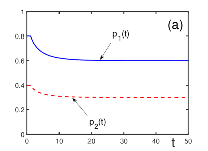
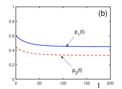
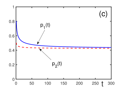
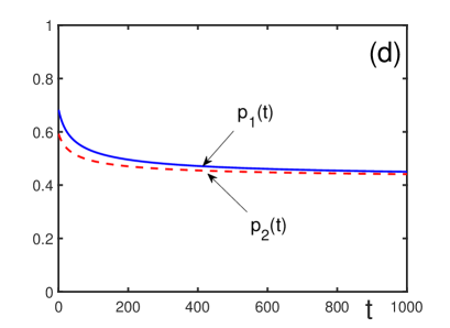
Figure 1: Long-term memory. Monotonically diminishing probabilities $p_{1}(t)$ (solid line) and $p_{2}(t)$ (dashed line) as functions of time: (a) Rational initial preference for $\varepsilon_{1}=\varepsilon_{2}=0$, the initial conditions are $f_{1}=0.6$, $f_{2}=0.3$, $q_{1}=0.2$, $q_{2}=0.1$, which implies $p_{1}(0)=0.8$ and $p_{2}(0)=0.4$. The limiting probabilities are $p_{1}(\infty)=f_{1}=0.6$ and $p_{2}(\infty)=f_{2}=0.3$. (b) Rational initial preference for $\varepsilon_{1}=0.5$, $\varepsilon_{2}=0.1$, the initial conditions are the same as in Fig. 1(a), which gives $p_{1}(0)=0.6$ and $p_{2}(0)=0.44$. The limiting probabilities are $p_{1}(\infty)=p_{1}^{*}=0.45$ and $p_{2}(\infty)=p_{2}^{*}=0.33$. (c) Irrational initial preference for $\varepsilon_{1}=\varepsilon_{2}=0$, the initial conditions are $f_{1}=0.3$, $f_{2}=0.4$, $q_{1}=0.5$, $q_{2}=0.1$, which implies $p_{1}(0)=0.8$ and $p_{2}(0)=0.5$. The consensual probabilities are $p_{1}(\infty)=p_{2}(\infty)=p^{*}=0.42$. (d) Irrational initial preference for $\varepsilon_{1}=0.4$, $\varepsilon_{2}=0.3$, the initial conditions are the same as in Fig. 1(c), which implies $p_{1}(0)=0.68$ and $p_{2}(0)=0.59$. The consensual probabilities are $p_{1}(\infty)=p_{2}(\infty)=p^{*}=0.42$.

follow. This is illustrated in Fig. 1 for the rational as well as irrational initial preferences. The information field decreases the difference between the probabilities at finite times, but they reach the same limiting values $p_{j}(\infty)$ at long times.

8.3 Monotonically increasing probabilities

In the case $\varepsilon_{1}=\varepsilon_{2}=0$, monotonically increasing probabilities occur if

$$q_{1}<0\;,\qquad q_{2}<0\qquad(\varepsilon_{j}=0\;,~{}~{}\forall~{}j)\;.$$ (76)

From this, the inequalities

$$(1-\varepsilon_{1})q_{1}+\varepsilon_{1}q_{2}<0\;,\qquad(1-\varepsilon_{2})q_{2}+\varepsilon_{2}q_{1}<0\;,$$ (77)

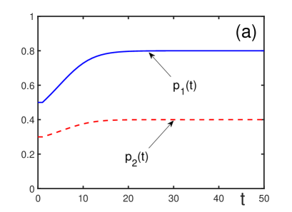
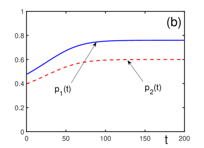
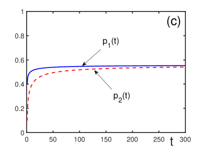
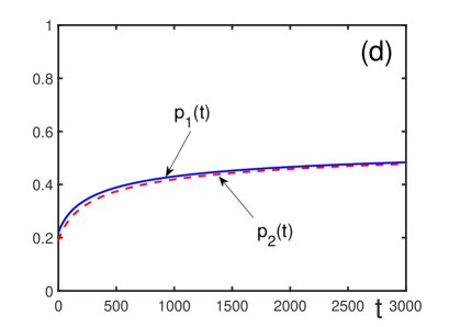
Figure 2: Long-term memory. Monotonically increasing probabilities $p_{1}(t)$ (solid line) and $p_{2}(t)$ (dashed line) as functions of time: (a) Rational initial preference for $\varepsilon_{1}=\varepsilon_{2}=0$, the initial conditions are $f_{1}=0.8$, $f_{2}=0.4$, $q_{1}=-0.3$, $q_{2}=-0.1$, which implies $p_{1}(0)=0.5$ and $p_{2}(0)=0.3$. The limiting probabilities are $p_{1}(\infty)=f_{1}=0.8$ and $p_{2}(\infty)=f_{2}=0.4$. (b) Rational initial preference for $\varepsilon_{1}=0.1$, $\varepsilon_{2}=0.5$, initial conditions are the same as for Fig. 2(a), which gives $p_{1}(0)=0.48$ and $p_{2}(0)=0.4$. The limiting probabilities are $p_{1}(\infty)=p_{1}^{*}=0.76$ and $p_{2}(\infty)=p_{2}^{*}=0.6$. (c) Irrational initial preference for $\varepsilon_{1}=\varepsilon_{2}=0$, initial conditions are $f_{1}=0.6$, $f_{2}=0.7$, $q_{1}=-0.2$, $q_{2}=-0.6$, which implies $p_{1}(0)=0.4$ and $p_{2}(0)=0.1$. The consensual probabilities are $p_{1}(\infty)=p_{2}(\infty)=p^{*}=0.55$. (d) Irrational initial preference for $\varepsilon_{1}=0.6$, $\varepsilon_{2}=0.3$, initial conditions are the same as for Fig. 2(c), which implies $p_{1}(0)=0.22$ and $p_{2}(0)=0.19$. The consensual probabilities are $p_{1}(\infty)=p_{2}(\infty)=p^{*}=0.55$.

for $0<\varepsilon_{j}<1$, follow. Therefore, the qualitative behaviour of the probabilities remains the same, they monotonically grow with time, as is shown in Fig. 2 for the rational and irrational initial preferences.

8.4 Probabilities diverging from each other

In the absence of information field, the probabilities diverge form each other when $p_{1}(t)$ increases while $p_{2}(t)$ decreases, which happens when

$$q_{1}<0\;,\qquad q_{2}>0\qquad(\varepsilon_{j}=0)\;.$$ (78)

Switching on the information field can essentially change the temporal behaviour of the probabilities. Thus choosing the parameters $\varepsilon_{j}$ so that

$$-\;\frac{q_{1}}{q_{2}-q_{1}}<\varepsilon_{1}<1\;,\qquad 0<\varepsilon_{2}<\frac{q_{2}}{q_{2}-q_{1}}$$ (79)

makes both probabilities diminishing. And for the case

$$0<\varepsilon_{1}<-\;\frac{q_{1}}{q_{2}-q_{1}}\;,\qquad\frac{q_{2}}{q_{2}-q_{1}}<\varepsilon_{2}<1$$ (80)

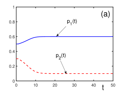
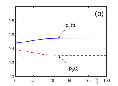
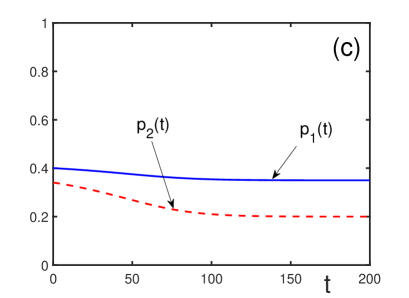
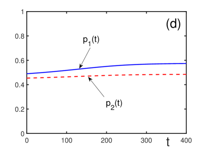
Figure 3: Long-term memory. Influence of the information field on probabilities $p_{1}(t)$ (solid line) and $p_{2}(t)$ (dashed line) diverging from each other, with the same initial conditions $f_{1}=0.6$, $f_{2}=0.1$, $q_{1}=-0.1$, and $q_{2}=0.2$: (a) Rational initial preference for $\varepsilon_{1}=\varepsilon_{2}=0$, which gives $p_{1}(0)=0.5$ and $p_{2}(0)=0.3$. The limiting probabilities are $p_{1}(\infty)=f_{1}=0.6$ and $p_{2}(\infty)=f_{2}=0.1$. (b) Rational initial preference for $\varepsilon_{1}=0.1$ and $\varepsilon_{2}=0.4$, which gives $p_{1}(0)=0.48$ and $p_{2}(0)=0.38$. The limiting probabilities are $p_{1}(\infty)=p_{1}^{*}=0.55$ and $p_{2}(\infty)=p^{*}=0.3$. (c) Rational initial preference for $\varepsilon_{1}=0.5$ and $\varepsilon_{2}=0.2$, which gives $p_{1}(0)=0.4$ and $p_{2}(0)=0.34$. The limiting probabilities are $p_{1}(\infty)=p_{1}^{*}=0.35$ and $p_{2}(\infty)=p_{2}^{*}=0.2$. (d) Rational initial preference for $\varepsilon_{1}=0.05$ and $\varepsilon_{2}=0.77$, which gives $p_{1}(0)=0.49$ and $p_{2}(0)=0.45$. The limiting probabilities are $p_{1}(\infty)=p_{1}^{*}=0.58$ and $p_{2}(\infty)=p_{2}^{*}=0.49$.

both probabilities increase, as is demonstrated in Fig. 3. In all cases, the probabilities diverge from each other.

8.5 Probabilities approaching each other

The probabilities approach each other if $p_{1}(t)$ decreases, while $p_{2}(t)$ increases, which occurs when

$$q_{1}>0\;,\qquad q_{2}<0\qquad(\varepsilon_{j}=0)\;.$$ (81)

Choosing the parameters of the information field such that

$$0<\varepsilon_{1}<\frac{q_{1}}{q_{1}-q_{2}}\;,\qquad-\;\frac{q_{2}}{q_{1}-q_{2}}<\varepsilon_{2}<1$$ (82)

makes both probabilities decreasing. And for the parameters in the range

$$\frac{q_{1}}{q_{1}-q_{2}}<\varepsilon_{1}<1\;,\qquad 0<\varepsilon_{2}<-\;\frac{q_{2}}{q_{1}-q_{2}}$$ (83)

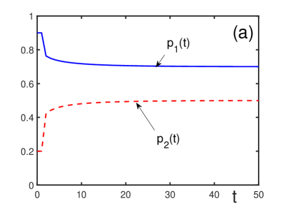
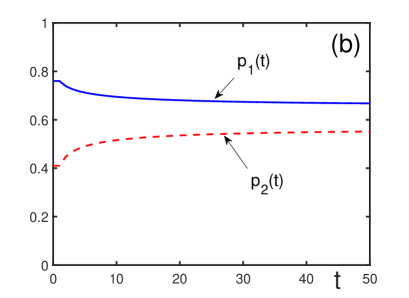
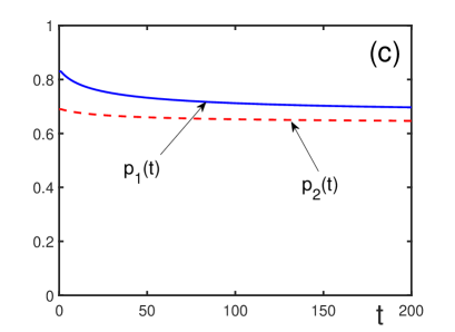
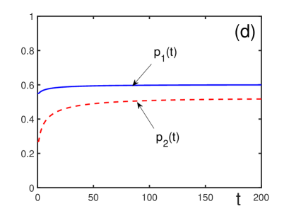
Figure 4: Long-term memory. Influence of the information field on probabilities $p_{1}(t)$ (solid line) and $p_{2}(t)$ (dashed line) approaching each other, in the case of the rational initial preference and the same initial conditions $f_{1}=0.7$, $f_{2}=0.5$, $q_{1}=0.2$, and $q_{2}=-0.3$: (a) $\varepsilon_{1}=\varepsilon_{2}=0$. The initial probabilities are $p_{1}(0)=0.9$ and $p_{2}(0)=0.2$. The limiting probabilities are $p_{1}(\infty)=f_{1}=0.7$ and $p_{2}(\infty)=f_{2}^{*}=0.5$. (b) $\varepsilon_{1}=0.2$ and $\varepsilon_{2}=0.3$. The initial probabilities are $p_{1}(0)=0.76$ and $p_{2}(0)=0.41$. The limiting probabilities are $p_{1}(\infty)=p_{1}^{*}=0.66$ and $p_{2}(\infty)=p_{2}^{*}=0.56$. (c) $\varepsilon_{1}=0.1$ and $\varepsilon_{2}=0.7$. The initial probabilities are $p_{1}(0)=0.83$ and $p_{2}(0)=0.69$. The limiting probabilities are $p_{1}(\infty)=p_{1}^{*}=0.68$ and $p_{2}(\infty)=p_{2}^{*}=0.64$. (d) $\varepsilon_{1}=0.5$ and $\varepsilon_{2}=0.1$. The initial probabilities are $p_{1}(0)=0.55$ and $p_{2}(0)=0.27$. The limiting probabilities are $p_{1}(\infty)=p_{1}^{*}=0.6$ and $p_{2}(\infty)=p_{2}^{*}=0.52$.

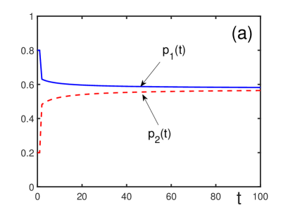
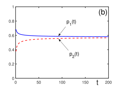
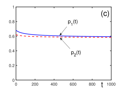
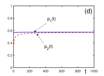
Figure 5: Long-term memory. Influence of the information field on probabilities $p_{1}(t)$ (solid line) and $p_{2}(t)$ (dashed line) approaching each other, in the case of the irrational initial preference and the same initial conditions $f_{1}=0.5$, $f_{2}=0.7$, $q_{1}=0.3$, and $q_{2}=-0.5$: (a) $\varepsilon_{1}=\varepsilon_{2}=0$. The initial probabilities are $p_{1}(0)=0.8$ and $p_{2}(0)=0.2$. The consensual limiting probabilities are $p_{1}(\infty)=p_{2}(\infty)=p^{*}=0.58$. (b) $\varepsilon_{1}=0.2$ and $\varepsilon_{2}=0.3$. The initial probabilities are $p_{1}(0)=0.68$ and $p_{2}(0)=0.38$. The consensual limiting probabilities are $p_{1}(\infty)=p_{2}(\infty)=p^{*}=0.58$. (c) $\varepsilon_{1}=0.2$ and $\varepsilon_{2}=0.7$. The initial probabilities are $p_{1}(0)=0.68$ and $p_{2}(0)=0.62$. The consensual limiting probabilities are $p_{1}(\infty)=p_{2}(\infty)=p^{*}=0.57$. (d) $\varepsilon_{1}=0.4$ and $\varepsilon_{2}=0.2$. The initial probabilities are $p_{1}(0)=0.56$ and $p_{2}(0)=0.32$. The consensual limiting probabilities are $p_{1}(\infty)=p_{2}(\infty)=p^{*}=0.57$.

both probabilities increase. The role of the information field is illustrated in Fig. 4 for the case of the rational initial preference and in Fig. 5 for the irrational initial preference. While the information field changes the temporal behaviour of the probabilities, they continue approaching each other.

8.6 Dynamic preference reversal

Under a special choice of parameters, the following interesting effect occurs. The parameters are taken such that $\varepsilon_{1}=\varepsilon_{1}=0$, with the initial conditions $f_{1}<f_{2}$, $q_{1}>0$, $q_{2}<0$, $f_{1}+q_{1}$ close to one, and $f_{2}+q_{2}\ll 1$. This corresponds to the case of the irrational initial preference, since

$$p_{1}(0)\gg p_{2}(0)\;,\qquad f_{1}<f_{2}\;.$$ (84)

At the first time step, the condition $p_{1}(1)>p_{2}(1)$ is still preserved. However, at the second step, the initial inequality reverses to $p_{1}(2)<p_{2}(2)$. After this, the probabilities tend to their limits

$$\lim_{t\rightarrow\infty}p_{j}(t)=f_{j}\qquad(\varepsilon_{j}=0)\;,$$ (85)

with different $f_{j}$. However, switching on the information field again drastically changes the behaviour of the probabilities that now tend to the common consensual limit

$$\lim_{t\rightarrow\infty}p_{j}(t)=p^{*}\qquad(\varepsilon_{j}>0)$$ (86)

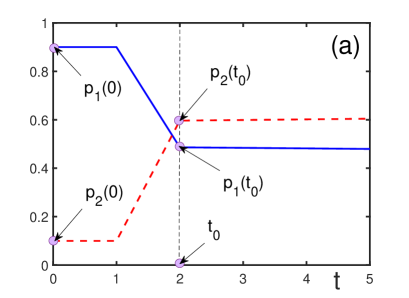
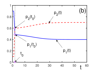
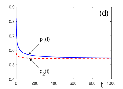
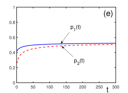
Figure 6: Long-term memory. Dynamic preference reversal under irrational initial preference. Probabilities $p_{1}(t)$ (solid line) and $p_{2}(t)$ (dashed line) for the initial conditions $f_{1}=0.4$, $f_{2}=0.7$, $q_{1}=0.5$, and $q_{2}=-0.6$. (a) The initial stage of the dynamic preference reversal for the time in the interval $0<t<5$, with $\varepsilon_{1}=\varepsilon_{2}=0$. The initial probabilities are $p_{1}(0)=0.9$ and $p_{2}(0)=0.1$. (b) Behavior of the probabilities after the preference reversal under $\varepsilon_{1}=\varepsilon_{2}=0$. The limiting probabilities are $p_{1}(\infty)=f_{1}=0.4$ and $p_{2}(\infty)=f_{2}=0.7$. (c) Switched on information field with $\varepsilon_{1}=0.1$ and $\varepsilon_{2}=0.1$. The consensual limiting probabilities are $p_{j}(t)=p^{*}=0.54$. (d) Switched on information field with $\varepsilon_{1}=0.1$ and $\varepsilon_{2}=0.6$. The consensual limiting probabilities are $p_{j}(t)=p^{*}=0.54$. (e) Switched on information field with $\varepsilon_{1}=0.6$ and $\varepsilon_{2}=0.2$. The consensual limiting probabilities are $p_{j}(t)=p^{*}=0.54$.

defined in equation (71). In that way, the existence of the common information in the society removes the effect of preference reversal, but leads to the consensual limit. This situation is shown in Fig. 6.

9 Agents with short-term memory

In the case of short-term memory, the available information reads

$$M_{j}(t)=\mu_{ji}(t)\qquad(i\neq j)\;.$$ (87)

9.1 General properties

Proposition 3. If the initial probabilities coincide,

$$p_{1}(0)=p_{2}(0)\;,$$ (88)

then they coincide for all times:

$$p_{1}(t)=p_{2}(t)\qquad(t=1,2,3,\ldots)\;.$$ (89)

Proof. Because of the initial condition (88), we have

$$\mu_{12}(0)=\mu_{21}(0)=0\;.$$

Therefore

$$p_{1}(1)=(1-\varepsilon_{1})[\;f_{1}+q_{1}(0)\exp\{-\mu_{12}(0)\}\;]+\varepsilon_{1}[\;f_{2}+q_{2}(0)\exp\{-\mu_{21}(0)\}\;]=$$

$$=(1-\varepsilon_{1})[\;f_{1}+q_{1}(0)\;]+\varepsilon_{1}[\;f_{2}+q_{2}(0)\;]=p_{1}(0)\;.$$

Similarly, we find

$$p_{2}(1)=p_{2}(0)\;.$$

Taking into account condition (88) gives

$$p_{1}(1)=p_{1}(0)=p_{2}(0)=p_{2}(1)\;.$$

From here

$$\mu_{12}(1)=\mu_{21}(1)=0\;.$$

Using this, we obtain

$$p_{1}(2)=(1-\varepsilon_{1})[\;f_{1}+q_{1}(0)\exp\{-\mu_{12}(1)\}\;]+\varepsilon_{1}[\;f_{2}+q_{2}(0)\exp\{-\mu_{21}(1)\}\;]=$$

$$=(1-\varepsilon_{1})[\;f_{1}+q_{1}(0)\;]+\varepsilon_{1}[\;f_{2}+q_{2}(0)\;]=p_{1}(0)\;,$$

which yields

$$p_{1}(2)=p_{1}(0)=p_{2}(0)=p_{2}(2)\;.$$

Continuing this chain of arguments, we come to equality (89). $\square$

9.2 Monotonic dynamics of probabilities

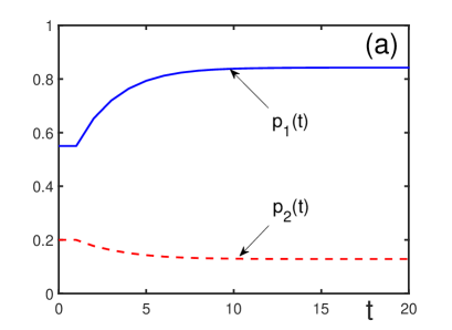
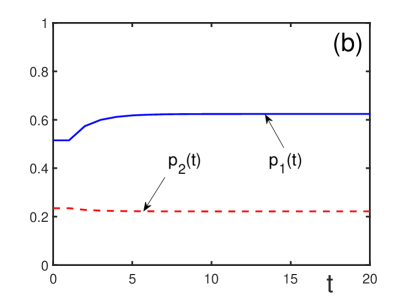
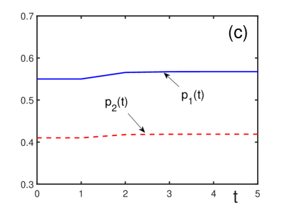
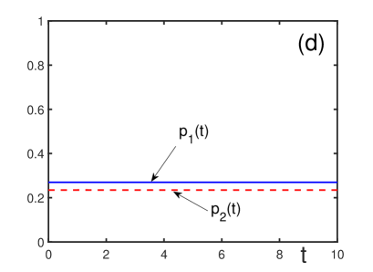
Figure 7: Short-term memory. Probabilities $p_{1}(t)$ (solid line) and $p_{2}(t)$ (dashed line). The initial conditions are $f_{1}=0.95$, $f_{2}=0.1$, $q_{1}=-0.4$, and $q_{2}=0.1$. (a) $\varepsilon_{1}=\varepsilon_{2}=0$. The initial probabilities are $p_{1}(0)=0.55$ and $p_{2}(0)=0.2$. The limiting probabilities are $p_{1}(\infty)=0.95$ and $p_{2}(\infty)=0.1$. (b) $\varepsilon_{1}=\varepsilon_{2}=0.1$. The initial probabilities are $p_{1}(0)=0.52$ and $p_{2}(0)=0.24$. The limiting probabilities are $p_{1}(\infty)=0.87$ and $p_{2}(\infty)=0.19$. (c) $\varepsilon_{1}=0$, $\varepsilon_{2}=0.6$. The initial probabilities are $p_{1}(0)=0.52$ and $p_{2}(0)=0.41$. The limiting probabilities are $p_{1}(\infty)=0.87$ and $p_{2}(\infty)=0.61$. (d) $\varepsilon_{1}=0.8$, $\varepsilon_{2}=0.1$. The initial probabilities are $p_{1}(0)=0.27$ and $p_{2}(0)=0.24$. The limiting probabilities are $p_{1}(\infty)=0.27$ and $p_{2}(\infty)=0.19$.

In the absence of the common information field, there are three main temporal regimes for the probabilities. One is the monotonic tendency of the probabilities to different limits. Switching on the information field does not change the monotonicity of the dynamics, but makes the probabilities closer to each other, as is clear from Fig. 7. The larger the parameters $\varepsilon_{j}$, characterizing the intensity of the information field, the closer to each other the probabilities. It looks rather natural that the common information in a society reduces the difference between the agent opinions.

9.3 Oscillatory dynamics of probabilities

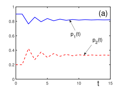
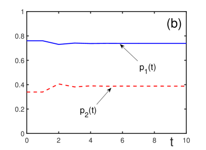
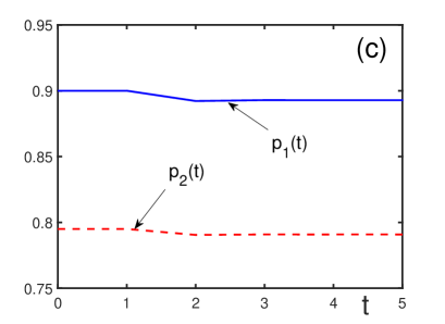
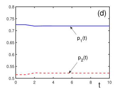
Figure 8: Short-term memory. Probabilities $p_{1}(t)$ (solid line) and $p_{2}(t)$ (dashed line). The initial conditions are $f_{1}=0.7$, $f_{2}=0.5$, $q_{1}=0.2$, and $q_{2}=-0.3$. (a) $\varepsilon_{1}=\varepsilon_{2}=0$. The initial probabilities are $p_{1}(0)=0.9$ and $p_{2}(0)=0.2$. The limiting probabilities are $p_{1}(\infty)=0.82$ and $p_{2}(\infty)=0.33$. (b) $\varepsilon_{1}=\varepsilon_{2}=0.2$. The initial probabilities are $p_{1}(0)=0.76$ and $p_{2}(0)=0.34$. The limiting probabilities are $p_{1}(\infty)=0.74$ and $p_{2}(\infty)=0.39$. (c) $\varepsilon_{1}=0$, $\varepsilon_{2}=0.85$. The initial probabilities are $p_{1}(0)=0.9$ and $p_{2}(0)=0.8$. The limiting probabilities are $p_{1}(\infty)=0.89$ and $p_{2}(\infty)=0.79$. (d) $\varepsilon_{1}=0.25$, $\varepsilon_{2}=0.45$. The initial probabilities are $p_{1}(0)=0.73$ and $p_{2}(0)=0.52$. The limiting probabilities are $p_{1}(\infty)=0.65$ and $p_{2}(\infty)=0.59$.

The convergence to the different limits $p_{j}(\infty)$ can be oscillatory in the absence of the common information field. Switching on the information field smoothes out the oscillations (but does not remove them completely), as is shown in Fig. 8. The stronger the influence of the common information, the smaller the oscillations. The oscillations can even disappear for sufficiently large parameters $\varepsilon_{j}$. This effect of smoothing the opinion oscillations caused by the common information in a strongly correlated society seems quite natural.

9.4 Everlasting probability oscillations

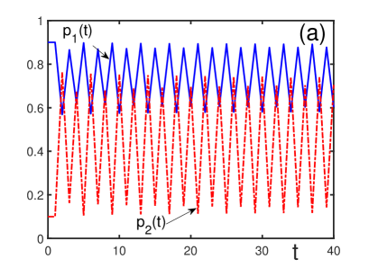
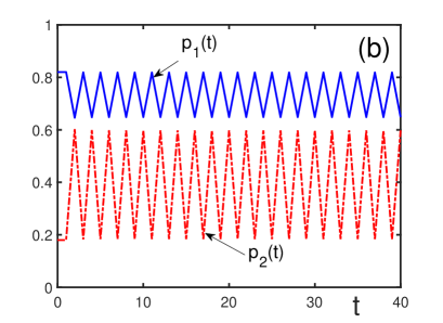
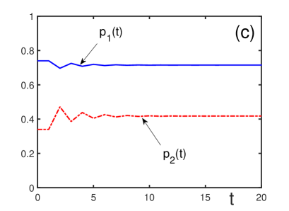
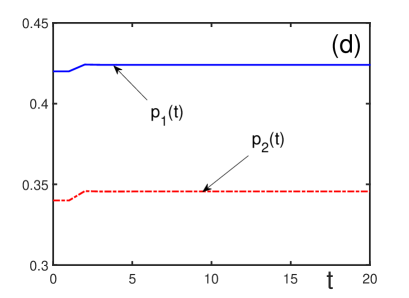
Figure 9: Short-term memory. Probabilities $p_{1}(t)$ (solid line) and $p_{2}(t)$ (dashed-dotted line). The initial conditions are $f_{1}=0.5$, $f_{2}=0.9$, $q_{1}=0.4$, and $q_{2}=-0.8$. (a) Everlasting oscillations for $\varepsilon_{1}=\varepsilon_{2}=0$. The initial conditions are $p_{1}(0)=0.9$ and $p_{2}(0)=0.1$. (b) Everlasting oscillations with reduced amplitude for $\varepsilon_{1}=\varepsilon_{2}=0.1$. The initial conditions are $p_{1}(0)=0.82$ and $p_{2}(0)=0.18$. (c) Oscillatory tendency to limits for $\varepsilon_{1}=0.2$, $\varepsilon_{2}=0.3$. The initial conditions are $p_{1}(0)=0.74$ and $p_{2}(0)=0.34$. The limiting probabilities are $p_{1}(\infty)=0.72$ and $p_{2}(\infty)=0.42$. (d) Monotonic tendency to limits for $\varepsilon_{1}=0.6$, $\varepsilon_{2}=0.3$. The initial conditions are $p_{1}(0)=0.42$ and $p_{2}(0)=0.34$. The limiting probabilities are $p_{1}(\infty)=0.424$ and $p_{2}(\infty)=0.346$.

When there is no common information field, the agents with a short-term memory can have their choice probabilities exhibiting a permanent oscillatory behaviour, without convergence to a fixed limit. This can be interpreted as agents who are hesitating without hope to converge to a clear decision. However switching on the information field reduces the amplitude of such oscillations. For sufficiently large information fields, the probabilities do not oscillate anymore and they converge to well defined limits. Again, such a smoothing effect of the common information in a society is understandable and very reasonable. These behaviours are shown in Fig. 9.

10 Dynamic disjunction effect

In the above sections, we have presented a complete classification of qualitatively different regimes of dynamic decision making for two groups of subjects choosing one of two given alternatives. In the real world, there exist various societies with rather different features. To our mind, the developed theory allows us to characterize practically any of the possible situations by fixing the appropriate society parameters. For concreteness, we study below the case where the so-called disjunction effect occurs, which violates the sure-thing principle [71, 72, 73, 74].

The disjunction effect was discovered by Tversky and Shafir [71] and confirmed in numerous studies (e.g. [72, 73, 74]). This effect is typical for two-step composite games of the following structure. At the first step, a group of subjects takes part in a game, where each member with equal probability can either win (event $B_{1}$) or lose (event $B_{2}$). At the second step, the agents are invited to participate in a second game, having the right either to accept the second game (event $A_{1}$) or to refuse it (event $A_{2}$). The second stage is realized in different variants: One can either accept or decline the second game under the condition of knowing the result of the first game. Or one can either accept or decline the second game without knowing the result of the first game.

In their experimental studies, Tversky and Shafir [71] find that the fraction of people accepting the second game, under the condition that the first game was won, and the fraction of those accepting the second game, under the condition that the first game was lost, respectively, are

$$f(A_{1}|B_{1})=0.69\;,\qquad f(A_{1}|B_{2})=0.59\;.$$ (90)

Here and below we denote classical probabilities by the letter $f$ to distinguish them from quantum probabilities denoted by the letter $p$. From the normalization condition for the conditional probabilities, we have

$$f(A_{2}|B_{1})=0.31\;,\qquad f(A_{2}|B_{2})=0.41\;.$$ (91)

Hence the related joint probabilities are

$$f(A_{1}B_{1})=0.345\;,\qquad f(A_{1}B_{2})=0.295\;,\qquad f(A_{2}B_{1})=0.155\;,\qquad f(A_{2}B_{2})=0.205\;,$$ (92)

using the fact that each member has equal probability to either winning (event $B_{1}$) or losing (event $B_{2}$), so that $f(B_{1})=f(B_{2})=0.5$.

The question of interest is: How many subjects will accept or decline the second game, when the result of the first game is not known to them? That is, one needs to define the behavioral probabilities of two alternative events

$$A_{1}B=A_{1}\bigcap\left(B_{1}\bigcup B_{2}\right)\;,\qquad A_{2}B=A_{2}\bigcap\left(B_{1}\bigcup B_{2}\right)\;.$$ (93)

The classical probabilities for these events are

$$f(A_{1}B)=f(A_{1}B_{1})+f(A_{1}B_{2})=0.64\qquad f(A_{2}B)=f(A_{2}B_{1})+f(A_{2}B_{2})=0.36\;,$$ (94)

which implies that, by classical theory, the probability of accepting the second game, not knowing the results of the first one, is larger than that of refusing the second game, not knowing the result of the first game. This, actually, is nothing but the sure-thing principle [75] telling that if $f(A_{1}B_{1})>f(A_{2}B_{1})$ and $f(A_{1}B_{2})>f(A_{2}B_{2})$, then $f(A_{1}B)>f(A_{2}B)$. To great surprise, Tversky and Shafir in their experiments [71] observe that human decision makers behave opposite to the prescription of the sure-thing principle, with the majority refusing the second game, if the result of the first one is not known,

$$p_{exp}(A_{1}B)=0.36\;,\qquad p_{exp}(A_{2}B)=0.64\;.$$ (95)

The magnitude of the disjunction effect is characterized by the difference between the fraction of agents choosing the alternative $A_{n}B$ and the corresponding utility factor,

$$p_{exp}(A_{1}B)-f(A_{1}B)=0.36-0.64=-0.28\;,$$

$$p_{exp}(A_{2}B)-f(A_{2}B)=0.64-0.36=0.28\;.$$ (96)

This difference measures the magnitude of the attraction factor.

The resolution of the disjunction effect in the frame of the quantum decision theory has been given in [42, 47], taking into account that the behavioral probability, according to quantum rules, includes a utility factor and an attraction factor. The latter was estimated using a noninformative prior, which resulted in the magnitude of the attraction factor $0.25$, close to the empirical value of $0.28$.

The above discussion of the disjunction effect keeps in mind decision making performed in a short interval of time and without information exchange between the agents. But when the agents are provided sufficiently long time during which they are allowed to exchange information between them, then the disjunction effect attenuates, in the sense that the initial difference

$$|\;p(A_{n}B)-f(A_{n}B)\;|=0.28\qquad(n=1,2)$$ (97)

becomes smaller with time. The disjunction-effect attenuation has been proved by numerous empirical observations [76, 77, 78, 79, 80, 81, 82, 83, 84, 85].

In order to study the dynamics of the disjunction effect, we have to resort to the equations of the theory developed above. The setup of Tversky and Shafir [71] can be captured by the evolution equations for the probability $p_{j}(t)$ of choosing the alternative $A_{1}B$ by the $j$-th agent at time $t$, which take the form

$$p_{1}(t+1)=(1-\varepsilon_{1})[\;f+q_{1}(t)\;]+\varepsilon_{1}[\;f+q_{2}(t)\;]\;,$$

$$p_{2}(t+1)=(1-\varepsilon_{2})[\;f+q_{2}(t)\;]+\varepsilon_{2}[\;f+q_{1}(t)\;]\;,$$ (98)

with the initial conditions

$$p_{1}(0)=(1-\varepsilon_{1})(f+q_{1})+\varepsilon_{1}(f+q_{2})\;,$$

$$p_{2}(0)=(1-\varepsilon_{2})(f+q_{2})+\varepsilon_{2}(f+q_{1})\;,$$ (99)

where $q_{j}\equiv q_{j}(0)$ and $f=0.64$. As is seen from the difference

$$p_{1}(0)-p_{2}(0)=(1-\varepsilon_{1}-\varepsilon_{2})(q_{1}-q_{2})\;,$$ (100)

switching on the information field, so that $0\leq\varepsilon_{1}+\varepsilon_{2}\leq 1$, makes the probabilities $p_{1}(t)$ and $p_{2}(t)$ closer to each other.

We solve equations (98) in the long-term memory case, where agents accumulate the information from the previous interactions with other agents. The numerical solution shows that both probabilities $p_{1}(t)$ and $p_{2}(t)$ always tend to the same consensual limit:

$$\lim_{t\rightarrow\infty}p_{1}(t)=\lim_{t\rightarrow\infty}p_{2}(t)=f\;,$$ (101)

while the attraction factors decrease with time,

$$\lim_{t\rightarrow\infty}q_{1}(t)=\lim_{t\rightarrow\infty}q_{2}(t)=0\;,$$ (102)

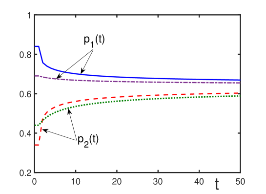
Figure 10: Disjunction effect attenuation as a function of time and its reduction caused by common information. The initial conditions are $f_{1}=f_{2}=f=0.64$, $q_{1}=0.2$, and $q_{2}=-0.3$. When $\varepsilon_{1}=\varepsilon_{2}=0$, functions $p_{1}(t)$ (solid line) and $p_{2}(t)$ (dashed line), under initial conditions $p_{1}(0)=0.84$ and $p_{2}(0)=0.34$, monotonically tend, with increasing time $t\rightarrow\infty$, to their common limit $f=0.64$. In the presence of the common information, with $\varepsilon_{1}=0.3$ and $\varepsilon_{2}=0.2$, the functions $p_{1}(t)$ (dashed-dotted line) and $p_{2}(t)$ (dotted line), under the initial conditions $p_{1}(0)=0.69$ and $p_{2}(0)=0.44$, monotonically tend to the same limit $f=0.64$ as $t\rightarrow\infty$. The common information reduces the disjunction effect from the beginning of the process.

thus diminishing the disjunction effect. This explains the disjunction effect attenuation observed in experiments [76, 77, 78, 79, 80, 81, 82, 83, 84, 85]. The information provided to decision makers reduces the difference between $p_{1}(t)$ and $p_{2}(t)$ at the very beginning of the process. See Fig. 10.

11 Conclusion

We have considered a network of agents taking decisions on the basis of quantum rules. This implies that the choice between several alternatives is characterized by the probabilities calculated using the techniques of quantum theory, which makes the process of choice multimodal. According to the quantum rules, decision makers take into account different features associated with the alternatives. The agents evaluate the utility of alternatives, characterized by utility factors as well as their attractiveness, described by attraction factors. They interact with other agents of the network by exchanging information and also they are influenced by the common information collectively created by the society members.

We consider two ways by which decision makers consume the available information, either accumulating the information from the previous interactions with other agents, or using the information only from one previous time step. The first case represents the presence of long-term memory and the second, short-term memory. Both these cases have been treated.

In order to understand the influence of the common information available in the society, we started from the situation where this common information is absent. Then we analyzed how the dynamics of taking decisions changes when the information field is switched on and its intensity is increased.

We have documented that the information field can essentially influence the temporal dynamics of the probabilities, whose values can be interpreted as the fraction of agents preferring one or the other alternative. Different variants of this influence have been carefully studied by varying initial conditions and different intensities of the common information field. We have treated the case of long-range interactions between the members of the society, keeping in mind that the members of the modern societies are able to exchange information at any distance through a number of means, such as phone, internet, mass media, etc.

In real life, there can exist various situations, quite diverse types of societies, and varying initial conditions. This is why our aim has been to present a complete analysis of different possible dynamic regimes and to examine the influence of the common information field on these regimes.

Summarizing the most important impact of the information field on the decision making dynamics in the network, we found that it smoothes out sharp variations in the temporal behaviour of the probabilities and can even remove them. For example, in the case of agents with long-term memory, we have documented the existence of a dynamic preference reversal where, starting from $p_{1}(0)>p_{2}(0)$, the dynamics gives at the second step an abrupt reversal to $p_{1}(2)<p_{2}(2)$, after which the probabilities tend to different limits $f_{j}$. Switching on the information field removes this reversal and makes the probabilities converging to a common consensual limit $p^{*}$.

For agents with short-term memory, the probabilities often tend to their limiting values through strong oscillations and, for a range of parameters, these oscillations last for ever, representing an ever lasting hesitation of the decision makers. However switching on the information field makes the amplitude of the oscillations smaller and even can halt the everlasting oscillations forcing the probabilities to converge to fixed limits.

The theory explains the attenuation of the disjunction effect with time, as a consequence of the exchange of information between the agents. This is embodied by the reduction of the magnitude of the attraction factors with increasing time. Additional common information further reduces the disjunction effect from the very beginning of the process.

Concluding, a society sharing a sufficiently large flow of common available information exhibits smoother dynamical processes of decision taking compared with a society without this common information. The common information removes sudden preference reversals in a society with long-term memory and can stop permanent decision oscillations in a society with short-term memory.

References

- [1] C.P. Williams, S.H. Clearwater, Explorations in Quantum Computing, Springer, New York, 1998.
- [2] M.A. Nielsen, I.L. Chuang, Quantum Computation and Quantum Information, Cambridge University, Cambridge, 2000.
- [3] V. Vedral, The role of relative entropy in quantum information theory, Rev. Mod. Phys. 74 (2002) 197–234.
- [4] M. Keyl, Fundamentals of quantum information theory, Phys. Rep. 369 (2002) 431–548.
- [5] O. Gühne, G. Toth, Entanglement detection, Phys. Rep. 474 (2009) 1–75.
- [6] M. Wilde, Quantum Information Theory, Cambridge University, Cambridge, 2013.
- [7] R. Albert, A.L. Barabasi, Statistical mechanics of complex networks, Rev. Mod. Phys. 74 (2002) 47–98.
- [8] R. Van Meter, Quantum Networking, Hoboken, Wiley, 2014.
- [9] H. Bernien et al., Probing many-body dynamics on a -atom quantum simulator, Nature 551 (2017) 579–584.
- [10] J. Zhang et al., Observation of a many-body dynamical phase transition with a -qubit quantum simulator, Nature 551 (2017) 601–604.
- [11] Y. Wu et al., Strong quantum computational advantage using a superconducting quantum processor, Phys. Rev. Lett. 127 (2021) 180501.
- [12] H.S. Zhong et al., Phase-programmable Gaussian boson sampling using stimulated squeezed light, Phys. Rev. Lett. 127 (2021) 180502.
- [13] A. Griesmaier, Generation of a dipolar Bose-Einstein condensate, J. Phys. B 40 (2007) R91–R134.
- [14] M.A. Baranov, Theoretical progress in many-body physics with ultracold dipolar gases, Phys. Rep. 464 (2008) 71–111.
- [15] M.A. Baranov, M. Dalmonte, G. Pupillo, P. Zoller, Condensed matter theory of dipolar quantum gases, Chem. Rev. 112 (2012) 5012–5061.
- [16] A. Boudjemâa, Properties of dipolar bosonic quantum gases at finite temperatures, J. Phys. A 49 (2016) 285005.
- [17] V.I. Yukalov, Dipolar and spinor bosonic systems, Laser Phys. 28 (2018) 053001.
- [18] K. Miakisz, E.W. Piotrowski, J. Sladkowski, Quantization of games: Towards quantum artificial intelligence, Theor. Comput. Sci. 358 (2006) 15–22.
- [19] M. Ying, Quantum computation, quantum theory and AI, Artif. Intell. 174 (2010) 162–176.
- [20] P. Wittek, Quantum Machine Learning, Academic, Amsterdam, 2014.
- [21] S. Bhattacharyya, U. Maulik, P. Dutta, Quantum Inspired Computational Intelligence, Morgan Kaufmann, Amsterdam, 2017.
- [22] M. Schuld, F. Petruccione, Supervised Learning with Quantum Computers, Springer, Cham, 2018.
- [23] S. Ganguly, Quantum Machine Learning: An Applied Approach, Springer, New York, 2021.
- [24] R. Penrose, The Emperor’s New Mind, Oxford, New York, 1989.
- [25] S. Hameroff, Quantum coherence in microtubules: A neural basis for emergent consciousness, J. Conscious Stud. 1 (1994) 91–118.
- [26] A. Khrennikov, On quantum-like probabilistic structure of mental information, Open Syst. Inf. Dynam. 11 (2004) 267–275.
- [27] A. Khrennikov, Quantum-like brain: Interference of minds, Bio. Syst. 84 (2006) 225–241.
- [28] V.I. Yukalov, D. Sornette, Quantum decision theory as quantum theory of measurement, Phys. Lett. A 372 (2008) 6867–6871.
- [29] V.I. Yukalov, D. Sornette, How brains make decisions, Springer Proc. Phys. 150 (2014) 37–53.
- [30] N. Nilsson, Artificial Intelligence: A New Synthesis, Morgan Kaufmann, San Francisco, 1998.
- [31] D. Poole, A. Mackworth, R. Goebel, Computational Intelligence: A Logical Approach, Oxford University, New York, 1998.
- [32] G.F. Luger, W.A. Stubblefield, Artificial Intelligence: Structures and Strategies for Complex Problem Solving, Benjamin Cummings, Redwood City, 2004.
- [33] E. Rich, K. Knight, S.B. Nair, Artificial Intelligence, McGraw Hill, New Delhi, 2009.
- [34] S.J. Russell, P. Norvig, Artificial Intelligence: A Modern Approach, Hoboken, Pearson, 2021.
- [35] A. Wichert, Principles of Quantum Artificial Intelligence, World Sientific, Singapore, 2013.
- [36] Y. Liang, W. Peng, Z.J. Zheng, O. Silven, G. Zhao, A hybrid quantum-classical neural network with deep residual learning, Neural Networks 143 (2021) 133–147.
- [37] M.J. Kewming, S. Shrapnel, G.J. Milburn, Designing a physical quantum agent, Phys. Rev. A 103 (2021) 032411.
- [38] J.B. Busemeyer, Z. Wang, J.T. Townsend, Quantum dynamics of human decision making, J. Math. Psychol. 50 (2006) 220–241.
- [39] M. Asano, M. Ohya, Y. Tanaka, A. Khrennikov, I. Basieva, On Application of Gorini-Kossakowski-Sudarshan-Lindblad Equation in Cognitive Psychology, Open Syst. Inf. Dynam. 18 (2011) 55–69.
- [40] M. Asano, A. Khrennikov, M. Ohya, Y. Tanaka, I. Yamato, Quantum Adaptivity in Biology: From Genetics to Cognition, Springer, Dordrecht, 2015.
- [41] F. Bagarello, I. Basieva, A. Khrennikov, Quantum field inspired model of decision making: Asymptotic stabilization of belief state via interaction with surrounding mental environment, J. Math. Psychol. 82 (2018) 159–168.
- [42] V.I. Yukalov, E.P. Yukalova, D. Sornette, Information processing by networks of quantum decision makers, Physica A 492 (2018) 747–766.
- [43] J. von Neumann, O. Morgenstern, Theory of Games and Economic Behavior, Princeton University, Princeton, 1953.
- [44] R.D. Luce, Individual Choice Behavior: A Theoretical Analysis, Wiley, New York, 1959.
- [45] V.I. Yukalov, D. Sornette, Scheme of thinking quantum systems, Laser Phys. Lett. 6 (2009) 833–839.
- [46] V.I. Yukalov, D. Sornette, Processing information in quantum decision theory, Entropy 11 1073–1120 (2009).
- [47] V.I. Yukalov, D. Sornette, Mathematical structure of quantum decision theory, Adv. Compl. Syst. 13 (2010) 659–698.
- [48] V.I. Yukalov, D. Sornette, Quantum probabilities of composite events in quantum measurements with multimode states, Laser Phys. 23 (2013) 105502.
- [49] A. Khrennikov, Towards information lasers, Entropy 17 (2015) 6969–6994.
- [50] A. Khrennikov, Z. Toffano, F. Dubois, Concept of information laser: From quantum theory to behavioural dynamics, Eur. Phys. J. Spec. Top. 227 (2019) 2133–2153.
- [51] D. Tsarev, A. Trofimova, A. Alodjants, A. Khrennikov, Phase transitions, collective emotions and decision-making problem in heterogeneous social systems, Sci. Rep. 9 (2019) 18039.
- [52] M.O. Jackson, Social and Economic Networks, Princeton University, Princeton, 2008.
- [53] M. Perc, J. Gómez-Gardeñes, A. Szolnoki, L.M. Floria, Y. Moreno, Evolutionary dynamics of group interactions on structured populations: a review, J. Roy. Soc. Interface 10 (2013) 20120997.
- [54] M. Perc, J.J. Jordan, D.G. Rand, Z. Wang, S. Boccaletti, A. Szolnoki, Statistical physics of human cooperation, Phys. Rep. 687 (2017) 1–51.
- [55] J. Von Neumann, Mathematical Foundations of Quantum Mechanics, Princeton University, Princeton, 1955.
- [56] V.I. Yukalov, D. Sornette, Manipulating decision making of typical agents, IEEE Trans. Syst. Man Cybern. Syst. 44 (2014) 1155–1168.
- [57] V.I. Yukalov, D. Sornette, Quantum probability and quantum decision making, Philos. Trans. Roy. Soc. A 374 (2016) 20150100.
- [58] V.I. Yukalov, D. Sornette, Quantum probabilities as behavioral probabilities, Entropy 19 (2017) 112.
- [59] V.I. Yukalov, D. Sornette, Quantitative predictions in quantum decision theory, IEEE Trans. Syst. Man Cybern. Syst. 48 (2018) 366–381.
- [60] M. Favre, A. Wittwer, H.R. Heinimann, V.I. Yukalov, D. Sornette, Quantum decision theory in simple risky choices, PLoS ONE 11 (2016) 0168045.
- [61] S. Vincent, T. Kovalenko, V.I. Yukalov, D. Sornette, Calibration of quantum decision theory: Aversion to large losses and predictability of probabilistic choices, http://ssrn.com/abstract=2775279 (2016).
- [62] G.M. Ferro, T. Kovalenko, D. Sornette, Quantum decision theory augments rank-dependent expected utility and cumulative prospect theory, J. Econ. Psychol. 86 (2021) 102417.
- [63] V.I. Yukalov, Entanglement measure for composite systems, Phys. Rev. Lett. 90 (2003) 167905.
- [64] V.I. Yukalov, Quantifying entanglement production of quantum operations, Phys. Rev. A 68 (2003) 022109.
- [65] V.I. Yukalov, E.P. Yukalova, V.A. Yurovsky, Entanglement production by statistical operators, Laser Phys. 29 (2019) 065502.
- [66] V.I. Yukalov, Equilibration of quasi-isolated quantum systems, Phys. Lett. A 376 (2012) 550–554.
- [67] V.I. Yukalov, Decoherence and equilibration under nondestructive measurements, Ann. Phys. (N.Y.) 327 (2012) 253–263.
- [68] S. Kullback, R.A. Leibler, On information and sufficiency, Ann. Math. Stat. 22 (1951) 79–86.
- [69] S. Kullback, Information Theory and Statistics, Wiley, New York, 1959.
- [70] W.H. Sandholm, Population Games and Evolutionary Dynamics, Massachusetts Institute of Technology, Cambridge, 2010.
- [71] A. Tversky, E. Shafir, The disjunction effect in choice under uncertainty, Psychol. Sci. 3 (1992) 305–309.
- [72] R.T.A. Croson, The disjunction effect and reason-based choice in games, Org. Behav. Human Decis. Process. 80 (1999) 118–133.
- [73] C. Lambdin, C. Burdsal, The disjunction effect reexamined: Relevant methodological issues and the fallacy of unspecified percentage comparisons, Org. Behav. Human Decis. Process. 103 (2007) 268–276.
- [74] S. Li, J.E. Taplin, Y. Zhang, The equate-to-differentiate way of seeing the prisoner’s dilemma, Inform. Sci. 177 (2007) 1395–1412.
- [75] L.J. Savage, The Foundations of Statistics, Wiley, New York, 1954.
- [76] A. Kühberger, D. Komunska, J. Perner, The disjunction effect: Does it exist for two-step gambles? Org. Behav. Hum. Decis. Process. 85 (2001) 250–264.
- [77] G. Charness, M. Rabin, Understanding social preferences with simple tests, Quart. J. Econ. 117 (2002) 817–869.
- [78] A. Blinder, J. Morgan, Are two heads better than one? An experimental analysis of group versus individual decision-making, J. Money Credit Bank. 37 (2005) 789–811.
- [79] D. Cooper, J. Kagel, Are two heads better than one? Team versus individual play in signaling games, Amer. Econ. Rev. 95 (2005) 477–509.
- [80] E. Tsiporkova, V. Boeva, Multi-step ranking of alternatives in a multi-criteria and multi-expert decision making environment, Inform. Sci. 176 (2006) 2673–2697.
- [81] G. Charness, E. Karni, D. Levin, Individual and group decision making under risk: an experimental study of bayesian updating and violations of first-order stochastic dominance, J. Risk Uncert. 35 (2007) 129–148.
- [82] G. Charness, L. Rigotti, A. Rustichini, Individual behavior and group membership, Amer. Econ. Rev. 97 (2007) 1340–1352.
- [83] Y. Chen, S. Li, Group identity and social preferences, Amer. Econ. Rev. 99 (2009) 431–457.
- [84] H.H. Liu, A.M. Colman, Ambiguity aversion in the long run: Repeated decisions under risk and uncertainty, J. Econ. Psychol. 30 (2009) 277–284.
- [85] G. Charness, E. Karni, D. Levin, On the conjunction fallacy in probability judgement: New experimental evidence regarding Linda, Games Econ. Behav. 68 (2010) 551–556.