The Newton method for affine phase retrieval

Abstract.

We consider the problem of recovering a signal from the magnitudes of affine measurements, which is also known as affine phase retrieval. In this paper, we formulate affine phase retrieval as an optimization problem and develop a second-order algorithm based on Newton method to solve it. Besides being able to convert into a phase retrieval problem, affine phase retrieval has its unique advantages in its solution. For example, the linear information in the observation makes it possible to solve this problem with second-order algorithms under complex measurements. Another advantage is that our algorithm doesn’t have any special requirements for the initial point, while an appropriate initial value is essential for most non-convex phase retrieval algorithms. Starting from zero, our algorithm generates iteration point by Newton method, and we prove that the algorithm can quadratically converge to the true signal without any ambiguity for both Gaussian measurements and CDP measurements. In addition, we also use some numerical simulations to verify the conclusions and to show the effectiveness of the algorithm.

1. Introduction

Phase retrieval problem arise in a wild range of applications in science and engineering, where one seeks to recover an image (a signal) or determine the structure of an object from various phaseless measurements, such as crystallography [19, 18], diffraction imaging [4], optics [21] and astronomy [9]. Symbolically, phase retrieval problem can be viewed as recovering a signal ${\mathbf{x}}\in{\mathbb{H}}^{n}$ (${\mathbb{H}}={\mathbb{C}}$ or ${\mathbb{R}}$) from a quadratic system:

(1.1) $$\{y_{j}=\lvert\langle{{\mathbf{a}}_{j},{\mathbf{x}}}\rangle\rvert^{2},j=1,\ldots,m\},$$

where $\{{\mathbf{a}}_{1},\ldots,{\mathbf{a}}_{m}\}\subset{\mathbb{H}}^{n}$ are the measurements and $y_{j},\,j=1,\ldots,m$ are the observations. For problem (1.1), since the signal multiplied by a unit constant does not change the observed value, it’s easy to find that any $e^{i\theta}{\mathbf{x}}$, $\theta\in[0,2\pi)$ is also a solution to the system, so the best we can do is to recover the signal ${\mathbf{x}}$ under a global phase factor. For classical phase retrieval, in which the measurements are Fourier transforms, it is more challenging to obtain the solution as there are extra trivial and non-trivial ambiguities [3]. To recover the signal, prior information such as positivity, sparsity [15, 16] and structured measurements [14, 5] are usually imposed in solving the phase retrieval problem.

Affine phase retrieval [10] is a related problem in which we aim to recover a signal from the magnitudes of linear measurements, i.e., to investigate how to recover a signal ${\mathbf{x}}\in{\mathbb{H}}^{n}$ from their affine quadratic measurements:

$$\{y_{j}=\lvert\langle{{\mathbf{a}}_{j},{\mathbf{x}}}\rangle+b_{j}\rvert^{2},j=1,\ldots,m\},$$

where $\{{\mathbf{a}}_{1},\ldots,{\mathbf{a}}_{m}\}\subset{\mathbb{H}}^{n}$ are the measurements and ${\mathbf{b}}=(b_{1},b_{2},\ldots,b_{m})^{\top}\in{\mathbb{H}}^{n}$ is a known vector. When the vector ${\mathbf{b}}=\boldsymbol{0}$ (zero vector), the problem is directly a phase retrieval problem. So affine phase retrieval can also be viewed as phase retrieval with side information. Affine phase retrieval arises in holography [17, 2]/phase retrieval with reference signal[1, 12, 13], phase retrieval with background information [8, 23]. In holographic phase retrieval, a known reference signal at a certain distance from the unknown signal of interest makes the recovery measurements linear. In phase retrieval with background information, the known part of the signal helps us to obtain the amplitudes of linear measurements.

In this paper, we propose to give a mathematical framework and develop a recovery algorithm for affine phase retrieval problem. Obviously, if we set $\tilde{{\mathbf{a}}}_{j}=\begin{pmatrix}{\mathbf{a}}_{j}&\overline{b_{j}}\end{pmatrix}^{\top}\in{\mathbb{H}}^{n+1}$ and $\tilde{{\mathbf{x}}}=\begin{pmatrix}{\mathbf{x}}&1\end{pmatrix}^{\top}\in{\mathbb{H}}^{n+1}$, then $\lvert\langle{{\mathbf{a}}_{j},{\mathbf{x}}}\rangle+b_{j}\rvert^{2}=\lvert\langle{\tilde{{\mathbf{a}}}_{j},\tilde{{\mathbf{x}}}}\rangle\rvert^{2}$, i.e., the affine quadratic measurements in ${\mathbf{x}}$ is the same as the quadratic measurements in $\tilde{{\mathbf{x}}}$. Thus, by this way, affine phase retrieval problem can be reformulated as a phase retrieval problem. On the other hand, if we know some elements of the signal in advance, e.g., for ${\mathbf{x}}=[{\mathbf{x}}_{1},{\mathbf{x}}_{2}]^{\top}\in{\mathbb{H}}^{n}$ assuming that ${\mathbf{x}}_{2}\in{\mathbb{H}}^{n-n_{1}}$ is known, then the measurements $|{\mathbf{a}}_{j}^{*}{\mathbf{x}}|^{2}=|{\mathbf{a}}_{j}^{*}(1:n_{1}){\mathbf{x}}_{1}+{\mathbf{a}}_{j}^{*}(n_{1}+1:n){\mathbf{x}}_{2}|^{2}$, which indicates that the phase retrieval problem can be rewritten as an affine phase retrieval problem. Although the two problems are interconvertible, there are fundamental differences. For example, the affine phase retrieval problem can recover the signal precisely while the phase retrieval cannot.

In recent years, many generative models with spectral initialization have been proposed for various phase retrieval problems [6, 7, 20, 22, 11]. These non-convex algorithms can be divided into two steps: the first step is to generate a good initial point, and then the second step is to refine the initial point gradually through first-order optimization methods. The commonly used models are as follows:

$$\min_{{{\mathbf{z}}}\in{\mathbb{C}}^{n}}\frac{1}{2m}\sum_{j=1}^{m}(\lvert\langle{{\mathbf{a}}_{j},{\mathbf{z}}}\rangle\rvert^{2}-y_{j})^{2}\,\,\text{,}\,\,\min_{{{\mathbf{z}}}\in{\mathbb{C}}^{n}}\frac{1}{2m}\sum_{j=1}^{m}(\lvert\langle{{\mathbf{a}}_{j},{\mathbf{z}}}\rangle\rvert-\sqrt{y_{j}})^{2},$$

or

$$\min_{{{\mathbf{z}}}\in{\mathbb{C}}^{n}}\frac{1}{2m}\sum_{j=1}^{m}\lvert\langle{{\mathbf{a}}_{j},{\mathbf{z}}}\rangle\rvert^{2}-y_{j}\log\big{(}\lvert\langle{{\mathbf{a}}_{j},{\mathbf{z}}}\rangle\rvert^{2}\big{)}.$$

For the analysis of the theoretical convergence of these non-convex algorithms, an appropriate initialization is crucial. Regarding affine phase retrieval, there are some algorithms given for Fourier measurements. In paper [2], the authors propose a referenced deconvolution algorithm, which transforms the problem into a linear deconvolution. In papers [13, 1], the authors use side information or reference signals to regularize the classical Fourier phase retrieval algorithms and demonstrate that the algorithm provides significant improvement over the original algorithm.

1.1. Targets and Motivations

In this paper, we aim at providing a non-convex formulation and developing a second-order algorithm to solve affine phase retrieval problem. When obtaining the measurements $\{y_{j}=\lvert\langle{{\mathbf{a}}_{j},{\mathbf{z}}}\rangle+b_{j}\rvert^{2},j=1,\ldots,m\}$, we reformulate the problem as:

(1.2) $$\min_{{{\mathbf{z}}}\in{\mathbb{C}}^{n}}f({\mathbf{z}})=\min_{{{\mathbf{z}}}\in{\mathbb{C}}^{n}}\frac{1}{2m}\sum_{j=1}^{m}(\lvert\langle{{\mathbf{a}}_{j},{\mathbf{z}}}\rangle+b_{j}\rvert^{2}-y_{j})^{2}.$$

Then we build up our algorithm based on solving (1.2).

Next we provide some insight as to why we expect to use second-order algorithms to solve affine phase retrieval problem. In paper [11], we use Gauss-Newton method to solve phase retrieval problem when the measurements are in the real number field. The same approach can’t be generally extended to the complex case because the Jacobi matrix is not invertible for complex measurements. In contrast, the corresponding Jacobi matrix for affine phase retrieval problem is invertible as long as the complex measurements are affine phase retrievable (Lemma 6.1). This makes it possible for the second-order algorithms to be used in solving affine phase retrieval problem in complex domains.

1.2. Contributions

Since the affine phase retrieval problem can be rewritten as a phase retrieval problem, all the algorithms used in phase retrieval can be used for affine phase retrieval. In particular, when ${\mathbf{b}}$ is a Gaussian random vector, the conclusions of most phase retrieval algorithms are also applicable to affine phase retrieval. By exploiting the linear observations, we give a second-order algorithm under complex measurements for affine phase retrieval problem. This is the first time a second-order algorithm has been proposed for affine phase retrieval. Our contributions are summarized as follows: This iterative algorithm can allow exact recovery of the signal under noiseless measurements. The sequence of iterates can quadratically converge to the exact solution, and there are no special requirements for initial value. Our contributions are summarized as follows:

• Based on solving (1.2), we develop an iterative algorithm to solve the affine phase retrieval problem.

• We prove that the algorithm can quadratically converge to the exact signal without any ambiguity.

• The algorithm converges for both real and complex observations and has no special requirements on initial point.

• The proof is given under the measurements following both the Gaussian model and the admissible CDPs model.

Remark 1.1.

In our algorithm, we use Newton method to solve (1.2). The same proof technique can also be used to prove the convergence of other second-order algorithms, such as the Gauss-Newton method.

1.3. Notations

Throughout the whole paper, we reserve $C$, $c$ and $\gamma$, and their indexed versions to denote positive constants, whose values may change at each occurrence. All the signals and measurements are given in the complex domain. We use ${\mathbf{x}}\in{\mathbb{C}}^{n}$ to represent the precise signal we want to recover and use ${\mathbf{z}}_{k}\in{\mathbb{C}}^{n}$ to represent the $k$-th iteration point. Without losing generality and to simplify the explanation, we shall assume $\|{\mathbf{x}}\|=1$. When no subscription is used, $\|\cdot\|$ denotes the Euclidian norm, i.e., $\|\cdot\|=\|\cdot\|_{2}$. Here we suppose the sampling vectors ${\mathbf{a}}_{j}\in{\mathbb{C}}^{n},\,j=1,\ldots,m$ are distributed according to Gaussian model (Definition (1.1)) or admissible CDPs model (Definition (1.2)). And ${\mathbf{b}}\in{\mathbb{C}}^{n}$ is a vector where each element is $b\in{\mathbb{C}}$ or each element is independently and identically distributed under a random distribution which is bounded by $|b|$, i.e., $|b_{j}|\leq|b|$. For a vector ${\mathbf{s}}$, we use ${\mathbf{s}}^{\top}$ to represent the transpose of ${\mathbf{s}}$, use ${\mathbf{s}}^{*}$ to represent the conjugate transpose of ${\mathbf{s}}$ and use $\overline{{\mathbf{s}}}$ to represent the conjugate of ${\mathbf{s}}$. Denote ${\mathbf{z}}_{k}$ as the $k$-th iteration point and $S_{k}$ as the line segment between ${\mathbf{z}}_{k}$ and ${\mathbf{x}}$, i.e.,

$$S_{k}\,:=\,\{t{\mathbf{x}}+(1-t){\mathbf{z}}_{k}:\,\,0\leq t\leq 1\}.$$

Definition 1.1 (Gaussian model).

We say that the sampling vectors follow the Gaussian model if each ${\mathbf{a}}_{j}\in{\mathbb{C}}^{n}\overset{i.i.d.}{\sim}\mathcal{N}(0,I/2)+i\mathcal{N}(0,I/2)$.

Definition 1.2 (Admissible coded diffraction patterns (CDPs) model).

We say that the sampling vectors follow the admissible CDPs model if ${\mathbf{a}}_{j}={\mathbf{a}}_{(l,k)}={\mathbf{a}}_{(\lceil j/n\rceil,\,(j\,\text{mod}\,n)-1)}=D_{l}{\mathbf{f}}_{k}$ ($1\leq l\leq L$, $0\leq k\leq n-1$), with $D_{l}$ be the diagonal matrix with the modulation pattern $d_{l}[t]$ $(t=1,\ldots,n)$ on the diagonal and ${\mathbf{f}}^{*}_{k}$ be the rows of the Discrete Fourier Transform (DFT) matrix. Here the patterns $d_{l}[t]$ are i.i.d. with each entries sampled from a symmetric distribution $d$. The distribution obeys $|d|\leq M$, ${\mathbb{E}}(d)=0$, ${\mathbb{E}}(d^{2})=0$, ${\mathbb{E}}(\lvert d\rvert^{4})=2{\mathbb{E}}(\lvert d\rvert^{2})^{2}$. Throughout this paper, we assume ${\mathbb{E}}(\lvert d\rvert^{2})=1$ and $|d|<\sqrt{6}$. For a fixed $l$, this model collects the DFT of the signal modulated by $d_{l}[t]$ $(t=1,\ldots,n)$. So the total number of measurements is $nL$. More details can be found in [6, 5].

1.4. Organization

The rest of the paper is organized as follows: In section 2, we develop the iterative algorithm for (1.2), which is based on Newton method. In section 3, we give the convergence analysis of the algorithm and prove that the algorithm has second-order convergence rate. In section 4, we provide some numerical tests to verify the conclusions we have obtained. In the end, some useful lemmas and proofs are given in the appendix.

2. The Algorithm-Newton Method

Suppose we have already obtained an initial guess ${\mathbf{z}}_{0}$ which satisfying $\|{\mathbf{x}}-{\mathbf{z}}_{0}\|\leq\sqrt{\delta}$ for a constant $\delta>0$, next we develop the Newton iterative step to solve the optimization problem (1.2).

Here function

$$f({\mathbf{z}})=\frac{1}{2m}\sum_{j=1}^{m}(\lvert\langle{{\mathbf{a}}_{j},{\mathbf{z}}}\rangle+b_{j}\rvert^{2}-y_{j})^{2}$$

is a real-valued function over complex variables and can be written in the form

$$f({\mathbf{z}},\overline{{\mathbf{z}}})=\frac{1}{2m}\sum_{j=1}^{m}(\overline{{\mathbf{z}}}^{\top}{\mathbf{a}}_{j}{\mathbf{a}}_{j}^{*}{\mathbf{z}}+2b_{j}\overline{{\mathbf{a}}}^{\top}{\mathbf{z}}+\lvert b_{j}\rvert^{2}-y_{j})^{2}.$$

Throughout the paper, we make use of the Wirtinger calculus and Wirtinger Derivatives, which use coordinates

$$\begin{bmatrix}{\mathbf{z}}\\ \overline{{\mathbf{z}}}\end{bmatrix}\in{\mathbb{C}}^{2n},\quad{\mathbf{z}}={\mathbf{z}}_{R}+i{\mathbf{z}}_{I}\quad\textup{and}\quad\overline{{\mathbf{z}}}={\mathbf{z}}_{R}-i{\mathbf{z}}_{I}$$

for complex variables instead of $({\mathbf{z}}_{R},{\mathbf{z}}_{I})\in{\mathbb{R}}^{2n}$ for brevity of expression.

2.1. Newton iteration

For the function $f({\mathbf{z}})$, given a vector ${\mathbf{z}}_{k}\in{\mathbb{C}}^{n}$ and incremental $\Delta{\mathbf{z}}_{k}={\mathbf{z}}-{\mathbf{z}}_{k}\in{\mathbb{C}}^{n}$ and we define the gradient and Hessian in a way based on Wirtinger Derivatives (more details can be found in paper [6]), such that the Taylor’s approximation takes the form

$$f({\mathbf{z}})=f({\mathbf{z}}_{k}+\Delta{\mathbf{z}}_{k})\approx f({\mathbf{z}}_{k})+\big{(}\nabla f({\mathbf{z}}_{k},\overline{{\mathbf{z}}_{k}})\big{)}^{*}\begin{pmatrix}\Delta{\mathbf{z}}_{k}\\ \Delta\overline{{\mathbf{z}}_{k}}\end{pmatrix}+\frac{1}{2}\begin{pmatrix}\Delta{\mathbf{z}}_{k}\\ \Delta\overline{{\mathbf{z}}_{k}}\end{pmatrix}^{*}\nabla^{2}f({\mathbf{z}}_{k},\overline{{\mathbf{z}}_{k}})\begin{pmatrix}\Delta{\mathbf{z}}_{k}\\ \Delta\overline{{\mathbf{z}}_{k}}\end{pmatrix}.$$

Then based on the current iteration ${\mathbf{z}}_{k}$, ${\mathbf{z}}_{k+1}$ can be obtained by solving

$$\min_{{\mathbf{z}}\in{\mathbb{C}}^{n}}f({\mathbf{z}}_{k})+\big{(}\nabla f({\mathbf{z}}_{k},\overline{{\mathbf{z}}_{k}})\big{)}^{*}\begin{pmatrix}{\mathbf{z}}-{\mathbf{z}}_{k}\\ \overline{{\mathbf{z}}}-\overline{{\mathbf{z}}_{k}}\end{pmatrix}+\frac{1}{2}\begin{pmatrix}{\mathbf{z}}-{\mathbf{z}}_{k}\\ \overline{{\mathbf{z}}}-\overline{{\mathbf{z}}_{k}}\end{pmatrix}^{*}\nabla^{2}f({\mathbf{z}}_{k},\overline{{\mathbf{z}}_{k}})\begin{pmatrix}{\mathbf{z}}-{\mathbf{z}}_{k}\\ \overline{{\mathbf{z}}}-\overline{{\mathbf{z}}_{k}}\end{pmatrix}.$$

Thus we get the Newton iteration

(2.3) $$\begin{pmatrix}{\mathbf{z}}_{k+1}\\ \overline{{\mathbf{z}}_{k+1}}\end{pmatrix}=\begin{pmatrix}{\mathbf{z}}_{k}\\ \overline{{\mathbf{z}}_{k}}\end{pmatrix}-\big{(}\nabla^{2}f({\mathbf{z}}_{k},\overline{{\mathbf{z}}_{k}})\big{)}^{-1}\nabla f({\mathbf{z}}_{k},\overline{{\mathbf{z}}_{k}}).$$

In detail,

$$\nabla f({\mathbf{z}}_{k},\overline{{\mathbf{z}}_{k}}) =\begin{pmatrix}(\partial f/\partial{\mathbf{z}})\big{|}_{{\mathbf{z}}={\mathbf{z}}_{k}}&(\partial f/\partial\overline{{\mathbf{z}}})\big{|}_{\overline{{\mathbf{z}}}=\overline{{\mathbf{z}}_{k}}}\end{pmatrix}^{*}$$

$$=\frac{1}{m}\sum_{j=1}^{m}\begin{pmatrix}\Big{(}\lvert{\mathbf{a}}_{j}^{*}{\mathbf{z}}_{k}+b_{j}\rvert^{2}-y_{j}\Big{)}({\mathbf{a}}_{j}^{*}{\mathbf{z}}_{k}+b_{j}){\mathbf{a}}_{j}\vspace{3mm}\\ \Big{(}\lvert{\mathbf{a}}_{j}^{*}{\mathbf{z}}_{k}+b_{j}\rvert^{2}-y_{j}\Big{)}({\mathbf{z}}_{k}^{*}{\mathbf{a}}_{j}+\overline{b_{j}})\overline{{\mathbf{a}}_{j}}\end{pmatrix}$$

and

$$\nabla^{2}f({\mathbf{z}}_{k},\overline{{\mathbf{z}}_{k}}) =\begin{pmatrix}\frac{\partial}{\partial{\mathbf{z}}}\Big{(}\frac{\partial f}{\partial{\mathbf{z}}}\Big{)}^{*}&\frac{\partial}{\partial\overline{{\mathbf{z}}}}\Big{(}\frac{\partial f}{\partial{\mathbf{z}}}\Big{)}^{*}\vspace{2mm}\\ \frac{\partial}{\partial{\mathbf{z}}}\Big{(}\frac{\partial f}{\partial\overline{{\mathbf{z}}}}\Big{)}^{*}&\frac{\partial}{\partial\overline{{\mathbf{z}}}}\Big{(}\frac{\partial f}{\partial\overline{{\mathbf{z}}}}\Big{)}^{*}\end{pmatrix}\Bigg{|}_{{\mathbf{z}}={\mathbf{z}}_{k},\overline{{\mathbf{z}}}=\overline{{\mathbf{z}}_{k}}}$$

$$=\frac{1}{m}\sum_{j=1}^{m}\begin{pmatrix}(2\lvert{\mathbf{a}}_{j}^{*}{\mathbf{z}}_{k}+b_{j}\rvert^{2}-y_{j}){\mathbf{a}}_{j}{\mathbf{a}}_{j}^{*}&({\mathbf{a}}_{j}^{*}{\mathbf{z}}_{k}+b_{j})^{2}{\mathbf{a}}_{j}{\mathbf{a}}_{j}^{\top}\vspace{3mm}\\ ({\mathbf{z}}_{k}^{*}{\mathbf{a}}_{j}+\overline{b_{j}})^{2}\overline{{\mathbf{a}}_{j}}{\mathbf{a}}_{j}^{*}&(2\lvert{\mathbf{a}}_{j}^{*}{\mathbf{z}}_{k}+b_{j}\rvert^{2}-y_{j})\overline{{\mathbf{a}}_{j}}{\mathbf{a}}_{j}^{\top}\end{pmatrix}.$$

In the next section, we will prove that under certain conditions the matrix $\nabla^{2}f({\mathbf{z}}_{k},\overline{{\mathbf{z}}_{k}})$ is invertible.

2.2. The Newton Method with Re-sampling

The algorithm proposed in this paper is simply using iteration (2.3) to generate the solution. In theoretical analysis, we need the current measurements to be independent of the last iteration point, so we resample the measurement matrix $A$ at each iteration step, as in paper [11]. We can achieve this by dividing the measurements ${\mathbf{a}}_{j}$, $b_{j}$ and observations $y_{j}$ into disconnected blocks of equal size and choosing one of them for each iteration.

Algorithm 1 The Newton Method with Re-sampling for Affine Phase Retrieval

Measurement matrix: $A\in{\mathbb{C}}^{m\times n}$ and a fixed vector ${\mathbf{b}}=(b,b,\ldots,b)\in{\mathbb{C}}^{n}$, observations: ${\mathbf{y}}\in{\mathbb{R}}^{m}$ and the required accuracy $\epsilon>0$.

1. Set $T=c\log\log\frac{1}{\epsilon}$, where $c$ is a sufficiently large constant.

2. Partition ${\mathbf{y}}$ and the corresponding rows of $A$ and the vector ${\mathbf{b}}$ into $T$ equal disjoint sets: $({\mathbf{y}}^{(0)},A^{(0)},{\mathbf{b}}^{(0)}),({\mathbf{y}}^{(1)},A^{(1)},{\mathbf{b}}^{(1)}),\ldots,({\mathbf{y}}^{(T)},A^{(T)},{\mathbf{b}}^{(T)})$. The number of rows in $A^{(j)}$ is $m^{\prime}=m/T$.

3. Choose ${\mathbf{z}}_{0}=\boldsymbol{0}$ as the initial guess.

4. For $k=0,1,\ldots,T-1$ do

   $$\begin{pmatrix}{\mathbf{z}}_{k+1}\\ \overline{{\mathbf{z}}_{k+1}}\end{pmatrix}=\begin{pmatrix}{\mathbf{z}}_{k}\\ \overline{{\mathbf{z}}_{k}}\end{pmatrix}-\big{(}\nabla^{2}f^{(k+1)}({\mathbf{z}}_{k},\overline{{\mathbf{z}}_{k}})\big{)}^{-1}\nabla f^{(k+1)}({\mathbf{z}}_{k},\overline{{\mathbf{z}}_{k}}),$$

   in which $f^{(k+1)}$ are defined by measurements in $({\mathbf{y}}^{(k+1)},A^{(k+1)},{\mathbf{b}}^{(k+1)})$.

5. End for

${\mathbf{z}}_{T}$.

In Algorithm 1, we set ${\mathbf{b}}$ to be a fixed vector whose entries are equal to $b$ ($b$ is a constant). We can alternatively assume that ${\mathbf{b}}$ is a random vector with independent elements that follow a same bounded distribution. In Step 3, the initial point can also be determined by a randomly chosen vector, for the sake of simplicity, we start from $\boldsymbol{0}$.

3. Convergence Property of the Newton Method with Re-sampling

To study the convergence of the algorithm, we observe two consecutive iterations when the current estimated value is independent of the measurements. Without loss of generality, we assume that $\|{\mathbf{x}}\|=1$. Before giving the main theorem, we first prove some useful lemmas. First, to ensure that the Newton iteration is well-defined, we prove that the matrix $\nabla^{2}f({\mathbf{z}},\overline{{\mathbf{z}}})$ is invertible under mild conditions.

3.1. Two crucial Lemmas

Lemma 3.1.

Suppose that $\|{\mathbf{z}}_{k}-{\mathbf{x}}\|\leq\sqrt{\delta}$, where ${\mathbf{z}}_{k},{\mathbf{x}}\in{\mathbb{C}}^{n}$ with $\|{\mathbf{x}}\|=1$ and $\delta\geq 0$ is a constant. Suppose that the measurement vectors ${\mathbf{a}}_{j}\in{\mathbb{C}}^{n}$, $j=1,\ldots,m$ are distributed according to Gaussian model or admissible CDPs model, which are independent with ${\mathbf{z}}_{k}$ and ${\mathbf{x}}$. Set ${\mathbf{b}}=(b,b,\ldots,b)\in{\mathbb{C}}^{n}$ with $|b|^{2}\geq 4(\|{\mathbf{x}}\|^{2}+\|{\mathbf{z}}_{k}\|^{2})\geq 4(2+\delta-2\sqrt{\delta})$. For any $\epsilon=1/12>0$ and $\gamma_{\epsilon}>0$, when the number of measurements $m\geq Cn\log n$ in the Gaussian model and $L\geq C\log^{3}n$ in the admissible CDPs model for a sufficiently large constant $C$, matrix $\nabla^{2}f({\mathbf{z}}_{k},\overline{{\mathbf{z}}_{k}})$ is invertible and

$$\lambda_{\min}(\nabla^{2}f({\mathbf{z}}_{k},\overline{{\mathbf{z}}_{k}}))\geq\frac{|b|^{2}}{4}$$

holds with probability at least $1-c_{1}\exp(-\gamma_{\epsilon}n)-c_{2}/n^{2}$ and $1-c_{3}(2L+1)/n^{3}$ for Gaussian and admissible CDPs, respectively. Here $c_{1}$, $c_{2}$ and $c_{3}$ are positive constants.

Proof.

Set $S=\nabla^{2}f({\mathbf{z}}_{k},\overline{{\mathbf{z}}_{k}})$ to simplify the symbol. Recall that

$$S=\nabla^{2}f({\mathbf{z}}_{k},\overline{{\mathbf{z}}_{k}})=\frac{1}{m}\sum_{j=1}^{m}\begin{pmatrix}(2\lvert{\mathbf{a}}_{j}^{*}{\mathbf{z}}_{k}+b_{j}\rvert^{2}-y_{j}){\mathbf{a}}_{j}{\mathbf{a}}_{j}^{*}&({\mathbf{a}}_{j}^{*}{\mathbf{z}}_{k}+b_{j})^{2}{\mathbf{a}}_{j}{\mathbf{a}}_{j}^{\top}\vspace{3mm}\\ ({\mathbf{z}}_{k}^{*}{\mathbf{a}}_{j}+\overline{b_{j}})^{2}\overline{{\mathbf{a}}_{j}}{\mathbf{a}}_{j}^{*}&(2\lvert{\mathbf{a}}_{j}^{*}{\mathbf{z}}_{k}+b_{j}\rvert^{2}-y_{j})\overline{{\mathbf{a}}_{j}}{\mathbf{a}}_{j}^{\top}\end{pmatrix}.$$

As vectors ${\mathbf{x}}$, ${\mathbf{z}}_{k}$ and scalars $b_{j}=b,\,j=1,\ldots,m$ are all independent of ${\mathbf{a}}_{j},\,j=1,\ldots,m$. So according to Lemma 6.4, we know the expectation

$${\mathbb{E}}(S) =\begin{pmatrix}(2\|{\mathbf{z}}_{k}\|^{2}-\|{\mathbf{x}}\|^{2}+|b|^{2})I_{n}+2{\mathbf{z}}_{k}{\mathbf{z}}_{k}^{*}-{\mathbf{x}}{\mathbf{x}}^{*}&2{\mathbf{z}}_{k}{\mathbf{z}}_{k}^{\top}\vspace{2mm}\\ 2\overline{{\mathbf{z}}_{k}}{\mathbf{z}}_{k}^{*}&(2\|{\mathbf{z}}_{k}\|^{2}-\|{\mathbf{x}}\|^{2}+|b|^{2})I_{n}+2\overline{{\mathbf{z}}_{k}}{\mathbf{z}}_{k}^{\top}-\overline{{\mathbf{x}}}{\mathbf{x}}^{\top}\end{pmatrix}$$

$$=\begin{pmatrix}(2\|{\mathbf{z}}_{k}\|^{2}-\|{\mathbf{x}}\|^{2}+|b|^{2})I_{n}-{\mathbf{x}}{\mathbf{x}}^{*}&\boldsymbol{0}\\ \boldsymbol{0}&(2\|{\mathbf{z}}_{k}\|^{2}-\|{\mathbf{x}}\|^{2}+|b|^{2})I_{n}-\overline{{\mathbf{x}}}{\mathbf{x}}^{\top}\end{pmatrix}+2\begin{pmatrix}{\mathbf{z}}_{k}\\ \overline{{\mathbf{z}}_{k}}\end{pmatrix}\begin{pmatrix}\overline{{\mathbf{z}}_{k}}&{\mathbf{z}}_{k}^{\top}\end{pmatrix}.$$

Based on Lemma 6.5, when $\epsilon=1/12>0$, $m\geq Cn\log n$ in Gaussian model and $L\geq C\log^{3}n$ in the admissible CDPs model for a sufficiently large constant $C$,

$$\|S-{\mathbb{E}}(S)\|\leq\frac{1}{12}\|{\mathbb{E}}(S)\|=\frac{1}{12}\lambda_{\max}({\mathbb{E}}(S))$$

holds with probability at least $1-c_{1}\exp(-\gamma n)-c_{2}/n^{2}$ and $1-c_{3}(2L+1)/n^{3}$ for the Gaussian and admissible CDPs, respectively. Here $c_{1}$, $c_{2}$ and $c_{3}$ are positive constants. Then using the Wely theorem, we have

$$|\lambda_{\min}(S)-\lambda_{\min}({\mathbb{E}}(S))|\leq\|S-{\mathbb{E}}(S)\|\leq\frac{1}{12}\lambda_{\max}({\mathbb{E}}(S)),$$

which implies that

(3.4) $$\lambda_{\min}(S)\geq\lambda_{\min}({\mathbb{E}}(S))-\frac{1}{12}\lambda_{\max}({\mathbb{E}}(S)).$$

To obtain the lower bound of $\lambda_{\min}(S)$, we only need to study the eigenvalues of ${\mathbb{E}}(S)$. For this Hermitian matrix ${\mathbb{E}}(S)$, set $2\|{\mathbf{z}}_{k}\|^{2}-\|{\mathbf{x}}\|^{2}+|b|^{2}=\beta$, ${\mathbf{x}}={\mathbf{u}}$ and ${\mathbf{z}}_{k}={\mathbf{v}}$, then

$${\mathbb{E}}(S)=\begin{pmatrix}\beta I_{n}-{\mathbf{u}}{\mathbf{u}}^{*}&\boldsymbol{0}\\ \boldsymbol{0}&\beta I_{n}-\overline{{\mathbf{u}}}{\mathbf{u}}^{\top}\end{pmatrix}+2\begin{pmatrix}{\mathbf{v}}\\ \overline{{\mathbf{v}}}\end{pmatrix}\begin{pmatrix}{\mathbf{v}}^{*}&{\mathbf{v}}^{\top}\end{pmatrix}.$$

When $|b|^{2}\geq 4(\|{\mathbf{x}}\|^{2}+\|{\mathbf{z}}_{k}\|^{2})$,

$$\beta=2\|{\mathbf{z}}_{k}\|^{2}-\|{\mathbf{x}}\|^{2}+|b|^{2}>\|{\mathbf{x}}\|^{2},$$

according to Lemma 6.6, we know that the matrix $E(S)$ is invertible. Besides, we have

(3.5) $$\lambda_{\min}({\mathbb{E}}(S)) =\beta-\|{\mathbf{x}}\|^{2}=|b|^{2}+2(\|{\mathbf{z}}_{k}\|^{2}-\|{\mathbf{x}}\|^{2})\geq\frac{|b|^{2}}{2},$$

(3.6) $$\lambda_{\max}({\mathbb{E}}(S)) \leq\beta+4\|{\mathbf{z}}_{k}\|^{2}=|b|^{2}+6\|{\mathbf{z}}_{k}\|^{2}-\|{\mathbf{x}}\|^{2}\leq 3|b|^{2}.$$

Putting (3.5) and (3.6) into (3.4), we obtain

$$\lambda_{\min}(S)\geq\lambda_{\min}({\mathbb{E}}(S))-\frac{1}{12}\lambda_{\max}({\mathbb{E}}(S))\geq\frac{|b|^{2}}{4}.$$

∎

Under conditions in Lemma 3.1, we showed that for each iteration ${\mathbf{z}}_{k}$, the Hessian matrix $\nabla^{2}f({\mathbf{z}}_{k},\overline{{\mathbf{z}}_{k}})$ is positive definite with minimum eigenvalue no less than $|b|/4$. In the following Lemma, we will commit to proving the Lipschitz property of $\nabla^{2}f({\mathbf{s}},\overline{{\mathbf{s}}})$.

Lemma 3.2.

Suppose that $\|{\mathbf{z}}_{k}-{\mathbf{x}}\|\leq\sqrt{\delta}$, where ${\mathbf{z}}_{k},{\mathbf{x}}\in{\mathbb{C}}^{n}$ with $\|{\mathbf{x}}\|=1$ and $\delta\geq 0$ is a constant. Suppose that the measurement vectors ${\mathbf{a}}_{j}\in{\mathbb{C}}^{n}$, $j=1,\ldots,m$ are distributed according to Gaussian model or admissible CDPs model, which are independent with ${\mathbf{z}}_{k}$ and ${\mathbf{x}}$. Then for any $\epsilon=1/12>0$ and $\gamma_{\epsilon}>0$, when $m\geq Cn\log n$ in the Gaussian model and $L\geq C\log^{3}n$ in the admissible CDPs model for a sufficiently large constant $C$,

$$\|\nabla^{2}f({\mathbf{s}}_{1},\overline{{\mathbf{s}}_{1}})-\nabla^{2}f({\mathbf{s}}_{2},\overline{{\mathbf{s}}_{2}})\|\leq L_{f}\begin{pmatrix}\|{\mathbf{s}}_{1}-{\mathbf{s}}_{2}\|\\ \|\overline{{\mathbf{s}}_{1}}-\overline{{\mathbf{s}}_{2}}\|\end{pmatrix}$$

holds with probability at least $1-c_{1}\exp(-\gamma_{\epsilon}n)-c_{2}/n^{2}$ and $1-c_{3}(2L+1)/n^{3}$ for the Gaussian and admissible CDPs, respectively. Here $c_{1},c_{2},c_{3},\gamma_{\epsilon}$ are positive constants, ${\mathbf{s}}_{1},{\mathbf{s}}_{2}\in S_{k}=\{t{\mathbf{x}}+(1-t){\mathbf{z}}_{k}:\,\,0\leq t\leq 1\}$ and $L_{f}=12(1+\epsilon)(1+\sqrt{\delta})=13(1+\sqrt{\delta})$.

Proof.

As before, we set $S=\nabla^{2}f({\mathbf{s}}_{1},\overline{{\mathbf{s}}_{1}})-\nabla^{2}f({\mathbf{s}}_{2},\overline{{\mathbf{s}}_{2}})$ for simplicity, then based on Lemma 6.4 we have

(3.7) $${\mathbb{E}}(S) =2\begin{pmatrix}(\|{\mathbf{s}}_{1}\|^{2}-\|{\mathbf{s}}_{2}\|^{2})I_{n}+{\mathbf{s}}_{1}{\mathbf{s}}_{1}^{*}-{\mathbf{s}}_{2}{\mathbf{s}}_{2}^{*}&{\mathbf{s}}_{1}{\mathbf{s}}_{1}^{\top}-{\mathbf{s}}_{2}{\mathbf{s}}_{2}^{\top}\vspace{2mm}\\ \overline{{\mathbf{s}}_{1}}{\mathbf{s}}_{1}^{*}-\overline{{\mathbf{s}}_{2}}{\mathbf{s}}_{2}^{*}&(\|{\mathbf{s}}_{1}\|^{2}-\|{\mathbf{s}}_{2}\|^{2})I_{n}+\overline{{\mathbf{s}}_{1}}{\mathbf{s}}_{1}^{\top}-\overline{{\mathbf{s}}_{2}}{\mathbf{s}}_{2}^{\top}\end{pmatrix}$$

$$=2\Big{[}(\|{\mathbf{s}}_{1}\|^{2}-\|{\mathbf{s}}_{2}\|^{2})I_{2n}+\begin{pmatrix}{\mathbf{s}}_{1}\\ \overline{{\mathbf{s}}_{1}}\end{pmatrix}\begin{pmatrix}{\mathbf{s}}_{1}^{*}&{\mathbf{s}}_{1}^{\top}\end{pmatrix}-\begin{pmatrix}{\mathbf{s}}_{2}\\ \overline{{\mathbf{s}}_{2}}\end{pmatrix}\begin{pmatrix}{\mathbf{s}}_{2}^{*}&{\mathbf{s}}_{2}^{\top}\end{pmatrix}\Big{]}.$$

By Cauchy-Schwarz inequality,

(3.8) $$\big{|}\|{\mathbf{s}}_{1}\|^{2}-\|{\mathbf{s}}_{2}\|^{2}\|\big{|} =\frac{1}{2}\big{|}({\mathbf{s}}_{1}+{\mathbf{s}}_{2})^{*}({\mathbf{s}}_{1}-{\mathbf{s}}_{2})+({\mathbf{s}}_{1}-{\mathbf{s}}_{2})^{*}({\mathbf{s}}_{1}+{\mathbf{s}}_{2})\big{|}$$

$$\leq\|{\mathbf{s}}_{1}+{\mathbf{s}}_{2}\|\|{\mathbf{s}}_{1}-{\mathbf{s}}_{2}\|.$$

And using the fact that $\|{\mathbf{s}}\|=\|\overline{{\mathbf{s}}}\|$, we have

(3.9) $$\Big{\|}\begin{pmatrix}{\mathbf{s}}_{1}\\ \overline{{\mathbf{s}}_{1}}\end{pmatrix}\begin{pmatrix}{\mathbf{s}}_{1}^{*}&{\mathbf{s}}_{1}^{\top}\end{pmatrix}-\begin{pmatrix}{\mathbf{s}}_{2}\\ \overline{{\mathbf{s}}_{2}}\end{pmatrix}\begin{pmatrix}{\mathbf{s}}_{2}^{*}&{\mathbf{s}}_{2}^{\top}\end{pmatrix}\Big{\|}$$

$$=\frac{1}{2}\Big{\|}\begin{pmatrix}{\mathbf{s}}_{1}+{\mathbf{s}}_{2}\\ \overline{{\mathbf{s}}_{1}}+\overline{{\mathbf{s}}_{2}}\end{pmatrix}\begin{pmatrix}{\mathbf{s}}_{1}^{*}-{\mathbf{s}}_{2}^{*}&{\mathbf{s}}_{1}^{\top}-{\mathbf{s}}_{2}^{\top}\end{pmatrix}+\begin{pmatrix}{\mathbf{s}}_{1}-{\mathbf{s}}_{2}\\ \overline{{\mathbf{s}}_{1}}-\overline{{\mathbf{s}}_{2}}\end{pmatrix}\begin{pmatrix}{\mathbf{s}}_{1}^{*}+{\mathbf{s}}_{2}^{*}&{\mathbf{s}}_{1}^{\top}+{\mathbf{s}}_{2}^{\top}\end{pmatrix}\Big{\|}$$

$$\leq 2\|{\mathbf{s}}_{1}+{\mathbf{s}}_{2}\|\begin{pmatrix}\|{\mathbf{s}}_{1}-{\mathbf{s}}_{2}\|\\ \|\overline{{\mathbf{s}}_{1}}-\overline{{\mathbf{s}}_{2}}\|\end{pmatrix}.$$

Inserting (3.8) and (3.9) into (3.7), we obtain

(3.10) $$\|{\mathbb{E}}(S)\|\leq 6(\|{\mathbf{s}}_{1}+{\mathbf{s}}_{2}\|)\begin{pmatrix}\|{\mathbf{s}}_{1}-{\mathbf{s}}_{2}\|\\ \|\overline{{\mathbf{s}}_{1}}-\overline{{\mathbf{s}}_{2}}\|\end{pmatrix}.$$

Besides, as ${\mathbf{s}}_{1},{\mathbf{s}}_{2}\in S_{k}:=\{t{\mathbf{x}}+(1-t){\mathbf{z}}_{k},t\in[0,1]\}$, $\|{\mathbf{z}}_{k}-{\mathbf{x}}\|\leq\sqrt{\delta}$, so we have

$$1-\sqrt{\delta}\leq\|{\mathbf{z}}_{k}\|\leq 1+\sqrt{\delta}$$

and

(3.11) $$\|{\mathbf{s}}_{1}+{\mathbf{s}}_{2}\|=\|(t_{1}+t_{2}){\mathbf{x}}+(2-t_{1}-t_{2}){\mathbf{z}}_{k}\|\leq 2(1+\sqrt{\delta}).$$

Combining (3.11) and (3.10), we have

(3.12) $$\|{\mathbb{E}}(S)\|\leq 12(1+\sqrt{\delta})\begin{pmatrix}\|{\mathbf{s}}_{1}-{\mathbf{s}}_{2}\|\\ \|\overline{{\mathbf{s}}_{1}}-\overline{{\mathbf{s}}_{2}}\|\end{pmatrix}.$$

According to Lemma 6.5, for $\epsilon=1/12>0$, $m\geq Cn\log n$ in Gaussian model and $L\geq C\log^{3}n$ in admissible CDPs with a sufficiently large constant $C$,

$$\|S-{\mathbb{E}}(S)\|\leq\epsilon\|{\mathbb{E}}(S)\|$$

i.e.,

$$\|S\|\leq(1+\epsilon)\|{\mathbb{E}}(S)\|\leq 12(1+\epsilon)(1+\sqrt{\delta})\begin{pmatrix}\|{\mathbf{s}}_{1}-{\mathbf{s}}_{2}\|\\ \|\overline{{\mathbf{s}}_{1}}-\overline{{\mathbf{s}}_{2}}\|\end{pmatrix}=13(1+\sqrt{\delta})\begin{pmatrix}\|{\mathbf{s}}_{1}-{\mathbf{s}}_{2}\|\\ \|\overline{{\mathbf{s}}_{1}}-\overline{{\mathbf{s}}_{2}}\|\end{pmatrix}$$

holds with probability at least $1-c_{1}\exp(-\gamma_{\epsilon}n)-c_{2}/n^{2}$ and $1-c_{3}(2L+1)/n^{3}$ for the Gaussian and admissible CDPs, respectively. Here $c_{1},c_{2},c_{3},\gamma_{\epsilon}$ are positive constants. ∎

3.2. The main Theorem

Based on Lemma 3.1 and Lemma 3.2, we are ready to obtain the main theorem, i.e., the algorithm converges quadratically to the optimal solution.

Theorem 3.1.

Let ${\mathbf{x}}\in{\mathbb{C}}^{n}$ with $\|{\mathbf{x}}\|=1$ be an arbitrary vector and suppose $\|{\mathbf{z}}_{k}-{\mathbf{x}}\|\leq\sqrt{\delta}$. Let $y_{j}=\lvert{\mathbf{a}}_{j}^{*}{\mathbf{x}}+b_{j}\rvert^{2}$, where ${\mathbf{a}}_{j}\in{\mathbb{C}}^{n}$, $j=1,\ldots,m$ are distributed according to Gaussian model or admissible CDPs model, which are independent with ${\mathbf{x}}$ and ${\mathbf{z}}_{k}$. Suppose ${\mathbf{b}}=(b,b,\ldots,b)^{\top}\in{\mathbb{C}}^{m}$ be fixed with $|b|^{2}\geq\max\{26\sqrt{\delta}(1+\sqrt{\delta}),4(2+\delta-2\sqrt{\delta})\}$. The ${\mathbf{z}}_{k+1}$ is defined by the update rule (2.3). Then when $m\geq Cn\log n$ in Gaussian model or $L\geq C\log^{3}n$ in admissible CDPs, with probability at least $1-c/n^{2}$ or $1-cL/n^{3}$, we have

(3.13) $$\|{\mathbf{z}}_{k+1}-{\mathbf{x}}\|\leq\beta\cdot\|{\mathbf{z}}_{k}-{\mathbf{x}}\|^{2}\leq\|{\mathbf{z}}_{k}-{\mathbf{x}}\|,$$

where

(3.14) $$\beta=(1+\sqrt{\delta})\frac{26}{|b|^{2}}\leq\frac{1}{\sqrt{\delta}}.$$

Proof.

As ${\mathbf{x}}$ is the solution to (1.2), so we have $\nabla f({\mathbf{x}},\overline{{\mathbf{x}}})=\boldsymbol{0}$. From the iteration step

$$\begin{pmatrix}{\mathbf{z}}_{k+1}\\ \overline{{\mathbf{z}}_{k+1}}\end{pmatrix}=\begin{pmatrix}{\mathbf{z}}_{k}\\ \overline{{\mathbf{z}}_{k}}\end{pmatrix}-(\nabla^{2}f({\mathbf{z}}_{k},\overline{{\mathbf{z}}_{k}}))^{-1}\nabla f({\mathbf{z}}_{k},\overline{{\mathbf{z}}_{k}}),$$

we have

$$\begin{pmatrix}{\mathbf{z}}_{k+1}-{\mathbf{x}}\\ \overline{{\mathbf{z}}_{k+1}}-\overline{{\mathbf{x}}}\end{pmatrix} =\begin{pmatrix}{\mathbf{z}}_{k}-{\mathbf{x}}\\ \overline{{\mathbf{z}}_{k}}-\overline{{\mathbf{x}}}\end{pmatrix}-(\nabla^{2}f({\mathbf{z}}_{k},\overline{{\mathbf{z}}_{k}}))^{-1}\Big{(}\nabla f({\mathbf{z}}_{k},\overline{{\mathbf{z}}_{k}})-\nabla f({\mathbf{x}},\overline{{\mathbf{x}}})\Big{)}$$

$$=(\nabla^{2}f({\mathbf{z}}_{k},\overline{{\mathbf{z}}_{k}}))^{-1}\Big{[}\nabla^{2}f({\mathbf{z}}_{k},\overline{{\mathbf{z}}_{k}})\begin{pmatrix}{\mathbf{z}}_{k}-{\mathbf{x}}\\ \overline{{\mathbf{z}}_{k}}-\overline{{\mathbf{x}}}\end{pmatrix}-\Big{(}\nabla f({\mathbf{z}}_{k},\overline{{\mathbf{z}}_{k}})-\nabla f({\mathbf{x}},\overline{{\mathbf{x}}})\Big{)}\Big{]}$$

$$=(\nabla^{2}f({\mathbf{z}}_{k},\overline{{\mathbf{z}}_{k}}))^{-1}\Big{[}\nabla^{2}f({\mathbf{z}}_{k},\overline{{\mathbf{z}}_{k}})\begin{pmatrix}{\mathbf{z}}_{k}-{\mathbf{x}}\\ \overline{{\mathbf{z}}_{k}}-\overline{{\mathbf{x}}}\end{pmatrix}-\int_{0}^{1}\nabla^{2}f({\mathbf{g}}_{k},\overline{{\mathbf{g}}_{k}})\begin{pmatrix}{\mathbf{z}}_{k}-{\mathbf{x}}\\ \overline{{\mathbf{z}}_{k}}-\overline{{\mathbf{x}}}\end{pmatrix}{\,\mathrm{d}}t\Big{]}$$

$$=(\nabla^{2}f({\mathbf{z}}_{k},\overline{{\mathbf{z}}_{k}}))^{-1}\Big{[}\int_{0}^{1}\big{(}\nabla^{2}f({\mathbf{z}}_{k},\overline{{\mathbf{z}}_{k}})-\nabla^{2}f({\mathbf{g}}_{k},\overline{{\mathbf{g}}_{k}})\big{)}\begin{pmatrix}{\mathbf{z}}_{k}-{\mathbf{x}}\\ \overline{{\mathbf{z}}_{k}}-\overline{{\mathbf{x}}}\end{pmatrix}{\,\mathrm{d}}t\Big{]}.$$

Here ${\mathbf{g}}_{k}={\mathbf{z}}_{k}+t({\mathbf{x}}-{\mathbf{z}}_{k}),\,t\in[0,1]$. Taking Euclidian norm on both sizes,

(3.15) $$\begin{pmatrix}\|{\mathbf{z}}_{k+1}-{\mathbf{x}}\|\\ \|\overline{{\mathbf{z}}_{k+1}}-\overline{{\mathbf{x}}}\|\end{pmatrix} \leq\|(\nabla^{2}f({\mathbf{z}}_{k},\overline{{\mathbf{z}}_{k}}))^{-1}\|\cdot\int_{0}^{1}\big{\|}\nabla^{2}f({\mathbf{z}}_{k},\overline{{\mathbf{z}}_{k}})-\nabla^{2}f({\mathbf{g}}_{k},\overline{{\mathbf{g}}_{k}})\big{\|}\begin{pmatrix}\|{\mathbf{z}}_{k}-{\mathbf{x}}\|\\ \|\overline{{\mathbf{z}}_{k}}-\overline{{\mathbf{x}}}\|\end{pmatrix}{\,\mathrm{d}}t$$

According to Lemma 3.2, with high probability we have

(3.16) $$\int_{0}^{1}\big{\|}\nabla^{2}f({\mathbf{z}}_{k},\overline{{\mathbf{z}}_{k}})-\nabla^{2}f({\mathbf{g}}_{k},\overline{{\mathbf{g}}_{k}})\big{\|}{\,\mathrm{d}}t$$

$$\leq L_{f}\int_{0}^{1}\begin{pmatrix}\|{\mathbf{z}}_{k}-{\mathbf{g}}_{k}\|\\ \|\overline{{\mathbf{z}}_{k}}-\overline{{\mathbf{g}}_{k}}\|\end{pmatrix}{\,\mathrm{d}}t$$

$$=L_{f}\begin{pmatrix}\|{\mathbf{z}}_{k}-{\mathbf{x}}\|\\ \|\overline{{\mathbf{z}}_{k}}-\overline{{\mathbf{x}}}\|\end{pmatrix}\int_{0}^{1}t{\,\mathrm{d}}t=\frac{L_{f}}{2}\begin{pmatrix}\|{\mathbf{z}}_{k}-{\mathbf{x}}\|\\ \|\overline{{\mathbf{z}}_{k}}-\overline{{\mathbf{x}}}\|\end{pmatrix},$$

with $L_{f}=13(1+\sqrt{\delta})$.

As $|b|^{2}\geq 4(2+\delta-2\sqrt{\delta})$, then based on Lemma 3.1, we have

(3.17) $$\|(\nabla^{2}f({\mathbf{z}}_{k},\overline{{\mathbf{z}}_{k}}))^{-1}\|\leq\frac{4}{|b|^{2}}$$

with high probability. Taking use of the fact that $\|{\mathbf{z}}_{k+1}-{\mathbf{x}}\|=\|\overline{{\mathbf{z}}_{k+1}}-\overline{{\mathbf{x}}}\|$, we only need to trace the first half elements. Then inserting (3.17), (3.16) into (3.15), we obtain

$$\|{\mathbf{z}}_{k+1}-{\mathbf{x}}\| \leq\frac{4}{|b|^{2}}\cdot\frac{L_{f}}{2}\|{\mathbf{z}}_{k}-{\mathbf{x}}\|^{2}$$

$$=(1+\sqrt{\delta})\frac{26}{|b|^{2}}\|{\mathbf{z}}_{k}-{\mathbf{x}}\|^{2}.$$

Based on requirement $|b|^{2}\geq 26\sqrt{\delta}(1+\sqrt{\delta})$, we also know

$$(1+\sqrt{\delta})\frac{26}{|b|^{2}}\leq\frac{1}{\sqrt{\delta}}.$$

Then $\|{\mathbf{z}}_{k+1}-{\mathbf{x}}\|\leq\frac{1}{\sqrt{\delta}}\|{\mathbf{z}}_{k}-{\mathbf{x}}\|^{2}\leq\|{\mathbf{z}}_{k}-{\mathbf{x}}\|\leq\sqrt{\delta}$, so that the results can be maintained as the iteration processes. ∎

For Algorithm 1, we further prove that if there are enough measurements and the value of $|b|^{2}$ is large enough, it can converge to the true signal quadratically.

Theorem 3.2.

Suppose that ${\mathbf{x}}\in{\mathbb{C}}^{n}$ with $\|{\mathbf{x}}\|=1$ is an arbitrary vector, and ${\mathbf{a}}_{j},\,j=1,\ldots,m$ are distributed according to Gaussian model or admissible CDPs model and ${\mathbf{b}}=(b,b,\ldots,b)^{\top}$ is fixed with $|b|^{2}\geq 52$. Suppose $\epsilon>0$ is the target accuracy. When $m\geq C\log\log\frac{1}{\epsilon}\cdot n\log n$ in Gaussian model or $L\geq C\log\log\frac{1}{\epsilon}\cdot\log^{3}n$ in admissible CDPs model for a sufficiently large constant $C$, with probability at least $1-\tilde{c}/n^{2}$ for Gaussian or $1-\tilde{c}L/n^{3}$ for admissible CDPs ($\tilde{c}>0$), Algorithm 1 generates ${\mathbf{z}}_{T}$ satisfying

$$\|{\mathbf{z}}_{T}-{\mathbf{x}}\|\leq\epsilon.$$

Proof.

In Algorithm 1, we choose $T=c\log\log\frac{1}{\epsilon}$ and $m^{\prime}\geq C_{1}n\log n$ in Gaussian model and $L^{\prime}\geq C_{1}\log^{3}n$ in admissible CDPs model, where $C_{1}$ is a constant depending on $C,c$. Starting from ${\mathbf{z}}_{0}=\boldsymbol{0}$, we have $\|{\mathbf{z}}_{0}-{\mathbf{x}}\|\leq 1=\sqrt{\delta}$ and we have $|b|^{2}\geq 52=\max\{26\sqrt{\delta}(1+\sqrt{\delta}),4(2+\delta-2\sqrt{\delta})\}$. Under these conditions, using the conclusion derived in Theorem 3.1 $T$ times, we conclude that

$$\|{\mathbf{z}}_{T}-{\mathbf{x}}\| \leq\beta\|{\mathbf{z}}_{T-1}-{\mathbf{x}}\|^{2}$$

$$\leq\beta^{2^{T}-1}\|{\mathbf{z}}_{0}-{\mathbf{x}}\|^{2^{T}}$$

$$\leq\epsilon$$

holds with probability at least $1-\tilde{c}/n^{2}$ for Gaussian model or $1-\tilde{c}L/n^{3}$ for admissible CDPs model. ∎

4. Numerical Simulations

We perform numerical tests on two types of measurements to illustrate the effectiveness of our method. All tests are performed in the complex domain. We take the dimension $n=128$ and the exact signal ${\mathbf{x}}\in{\mathbb{C}}^{128}$.

4.1. Convergence Rate

We first verify the quadratic convergence rate of our algorithm. In the first test, we take $m=4n$ for Gaussian model and $L=6$ in admissible CDPs. Set $b=52\|{\mathbf{x}}\|$ and initial point ${\mathbf{z}}_{0}=\boldsymbol{0}$. We use the relative error $\|{\mathbf{x}}-{\mathbf{z}}_{k}\|/\|{\mathbf{x}}\|$ to measure the recovery performance of the algorithm. Figure 1 illustrates the quadratic convergence of our algorithm.

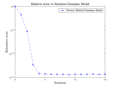
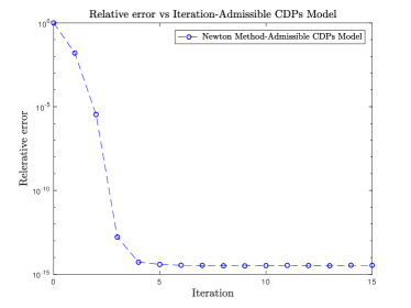
Figure 1. Convergence experiments: record the relative error of each iteration step. Here $n=128$ and $m=4n$ in (a) Gaussian model and $L=6$ in (b) admissible CDPs model.

4.2. Success Rate

Theoretically, to obtain accurate recovery, the number of measurements we need is $\mathcal{O}(n\log n)$ in Gaussian model or $\mathcal{O}(n\log^{3}n)$ in admissible CDPs model. In this test, we vary the number of measurements and record the success rate for each $m/n$ or $L$. Here for each $m/n$ or $L$, we perform 100 replicates to calculate the success rate. In our experiments, we set the maximum number of iterations to 15 and claim that a trial is successful when the relative error is less than $10^{-5}$. For Gaussian model, $m/n$ was varied in the range [1,5] with a step size $0.1$. For admissible CDPs model, $L$ was varied in the range [3,10] with a step size $1$. The results are shown in Figure 2, indicating that we do not need so many observations in practice.

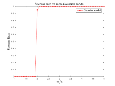
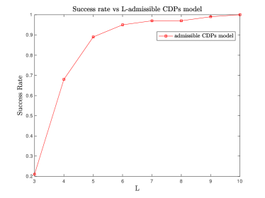
Figure 2. Success rate: record the success rate under 100 trials of different measurement numbers. Here $n=128$ and $m/n\in[1,6]$ in (a) Gaussian model and $L\in[3,10]$ in (b) admissible CDPs model.

5. Conclusions

In this paper, we reformulate the affine phase retrieval as an optimization problem and develop a second-order algorithm, the Newton method with resampling, to solve it. Starting from zero, the algorithm iteratively refines the estimate value by Newton method. When the measurements follow the Gaussian model or the admissible CDPs model, we proved that the algorithm converges quadratically to the exact solution. Using these analytical techniques, we can also develop other second-order algorithms for affine phase retrieval.

6. Appendix

Lemma 6.1.

[Theorem 3.1 in [10]] Let $A=({\mathbf{a}}_{1},\ldots,{\mathbf{a}}_{m})^{\top}\in{\mathbb{C}}^{m\times n}$ and ${\mathbf{b}}=(b_{1},\ldots,b_{m})^{\top}\in{\mathbb{C}}^{m}$. Viewing $\mathbf{M}_{A,{\mathbf{b}}}^{2}:=(|{\mathbf{a}}_{1}^{*}{\mathbf{x}}+b_{1}|^{2},\ldots,|{\mathbf{a}}_{m}^{*}{\mathbf{x}}+b_{m}|^{2})$ as a map ${\mathbb{C}}^{d}\longrightarrow{\mathbb{R}}^{m}$. Then $(A,{\mathbf{b}})$ is affine phase retrievable for ${\mathbb{C}}^{d}$ is equivalent with the real Jacobian of map $\mathbf{M}_{A,{\mathbf{b}}}^{2}$ has rank $2n$ for all ${\mathbf{x}}\in{\mathbb{C}}^{n}$.

Lemma 6.2.

[Lemma 7.4 in [6]] Suppose a signal ${\mathbf{x}}\in{\mathbb{C}}^{n}$ with $\|{\mathbf{x}}\|=1$ is independent from the measurement samples ${\mathbf{a}}_{j}\in{\mathbb{C}}^{n}$, $j=1,2,\ldots,m$. Assume that the vectors ${\mathbf{a}}_{j}$ are distributed according to either the Gaussian model or admissible CDPs model. Set matrix

$$S:=\frac{1}{m}\sum_{j=1}^{m}\begin{pmatrix}\lvert{\mathbf{a}}_{j}^{*}{\mathbf{x}}\rvert^{2}{\mathbf{a}}_{j}{\mathbf{a}}_{j}^{*}&({\mathbf{a}}_{j}^{*}{\mathbf{x}})^{2}{\mathbf{a}}_{j}{\mathbf{a}}_{j}^{\top}\vspace{3mm}\\ ({\mathbf{x}}^{*}{\mathbf{a}}_{j})^{2}\overline{{\mathbf{a}}_{j}}{\mathbf{a}}_{j}^{*}&\lvert{\mathbf{a}}_{j}^{*}{\mathbf{x}}\rvert^{2}\overline{{\mathbf{a}}_{j}}{\mathbf{a}}_{j}^{\top}\end{pmatrix}.$$

When the number of samples obeys $m\geq C_{\delta}n\log n$ in the Gaussian model and the number of patterns obeys $L\geq C_{\delta}\log^{3}n$ in the admissible CDPs model for a sufficiently large constant $C_{\delta}$,

$$\|S-{\mathbb{E}}(S)\|\leq\delta\|{\mathbb{E}}(S)\|$$

holds with probability at least $1-10\exp(-\gamma_{\delta}n)-8/n^{2}$ and $1-(2L+1)/n^{3}$ for the Gaussian and admissible CDPs, respectively.

Lemma 6.3.

[Lemma 7.8 in [6]] In the setup of Lemma 6.2,

$$\|I_{n}-\frac{1}{m}\sum_{j=1}^{m}{\mathbf{a}}_{j}{\mathbf{a}}_{j}^{*}\|\leq\epsilon$$

holds with probability at least $1-2\exp(-\gamma_{\epsilon}m)$ for the Gaussian model and $1-1/n^{2}$ for the admissible CDPs model.

Lemma 6.4.

Suppose that the signal ${\mathbf{x}}\in{\mathbb{C}}^{n}$ with $\|{\mathbf{x}}\|=1$ is independent from the measurement samples ${\mathbf{a}}_{j}$, $j=1,\ldots,m$. Assume that the vectors ${\mathbf{a}}_{j}$, $j=1,\ldots,m$ are distributed according to either the Gaussian model or admissible CDPs model. Set ${\mathbf{b}}=(b_{1},b_{2},\ldots,b_{m})\in{\mathbb{C}}^{m}$ be a fixed vector with each entries equal $b\in{\mathbb{C}}$. Define matrix

$$S:=\frac{1}{m}\sum_{j=1}^{m}\begin{pmatrix}\lvert{\mathbf{a}}_{j}^{*}{\mathbf{x}}+b_{j}\rvert^{2}{\mathbf{a}}_{j}{\mathbf{a}}_{j}^{*}&({\mathbf{a}}_{j}^{*}{\mathbf{x}}+b_{j})^{2}{\mathbf{a}}_{j}{\mathbf{a}}_{j}^{\top}\vspace{3mm}\\ ({\mathbf{x}}^{*}{\mathbf{a}}_{j}+\overline{b_{j}})^{2}\overline{{\mathbf{a}}_{j}}{\mathbf{a}}_{j}^{*}&\lvert{\mathbf{a}}_{j}^{*}{\mathbf{x}}+b_{j}\rvert^{2}\overline{{\mathbf{a}}_{j}}{\mathbf{a}}_{j}^{\top}\end{pmatrix}.$$

Then we have

$${\mathbb{E}}(S) =\begin{pmatrix}(\|{\mathbf{x}}\|^{2}+|b|^{2})I_{n}+{\mathbf{x}}{\mathbf{x}}^{*}&2{\mathbf{x}}{\mathbf{x}}^{\top}\vspace{2mm}\\ 2\overline{{\mathbf{x}}}{\mathbf{x}}^{*}&(\|{\mathbf{x}}\|^{2}+|b|^{2})I_{n}+\overline{{\mathbf{x}}}{\mathbf{x}}^{\top}\end{pmatrix}.$$

Proof.

1. The Gaussian Model:

As vector ${\mathbf{x}}$ and scalars $b_{j}=b,\,j=1,\ldots,m$ are all independent of ${\mathbf{a}}_{j},\,j=1,\ldots,m$. So the expectation of $\lvert{\mathbf{a}}_{1}^{*}{\mathbf{x}}+b_{1}\rvert^{2}{\mathbf{a}}_{1}{\mathbf{a}}_{1}^{*}$ is equal to $\lvert{\mathbf{a}}^{*}{\mathbf{x}}+b\rvert^{2}{\mathbf{a}}{\mathbf{a}}^{*}$, in which ${\mathbf{a}}=(a_{1},\ldots,a_{n})^{\top}\in{\mathbb{C}}^{n}$ is a Gaussian random vector. By definition

$$\lvert{\mathbf{a}}^{*}{\mathbf{x}}+b\rvert^{2}=\big{(}\sum_{i=1}^{n}\overline{a_{i}}x_{i}+b\big{)}\big{(}\sum_{j=1}^{n}a_{j}\overline{x_{j}}+\overline{b}\big{)}=\sum_{i}\sum_{j}\overline{a_{i}}a_{j}x_{i}\overline{x_{j}}+\overline{b}\sum_{i}\overline{a_{i}}x_{i}+b\sum_{j}a_{j}\overline{x_{j}}+\lvert b\rvert^{2},$$

then

$$\lvert{\mathbf{a}}^{*}{\mathbf{x}}+b\rvert^{2}{\mathbf{a}}{\mathbf{a}}^{*}=\Big{(}\sum_{i}\sum_{j}\overline{a_{i}}a_{j}x_{i}\overline{x_{j}}+\overline{b}\sum_{i}\overline{a_{i}}x_{i}+b\sum_{j}a_{j}\overline{x_{j}}+\lvert b\rvert^{2}\Big{)}\begin{pmatrix}\lvert a_{1}\rvert^{2}&a_{1}\overline{a_{2}}&\cdots&a_{1}\overline{a_{n}}\\ a_{2}\overline{a_{1}}&\lvert a_{2}\rvert^{2}&\cdots&a_{2}\overline{a_{n}}\\ \vdots&\vdots&\ddots&\vdots\\ a_{n}\overline{a_{1}}&a_{n}\overline{a_{2}}&\cdots&\lvert a_{n}\rvert^{2}\end{pmatrix}.$$

For matrix $\lvert{\mathbf{a}}^{*}{\mathbf{x}}+b\rvert^{2}{\mathbf{a}}{\mathbf{a}}^{*}$, first consider the expectation of diagonal elements $s_{k,k}$ with $k=1,2,\ldots,n$,

$${\mathbb{E}}(s_{k,k})= {\mathbb{E}}\Big{(}\big{(}\sum_{i}\sum_{j}\overline{a_{i}}a_{j}x_{i}\overline{x_{j}}+\overline{b}\sum_{i}\overline{a_{i}}x_{i}+b\sum_{j}a_{j}\overline{x_{j}}+\lvert b\rvert^{2}\big{)}|a_{k}|^{2}\Big{)}$$

$$={\mathbb{E}}\Big{(}\sum_{i=j=k}|a_{k}|^{4}|x_{k}|^{2}+\sum_{i=j\neq k}|a_{i}|^{2}|a_{k}|^{2}|x_{i}|^{2}+|b|^{2}|a_{k}|^{2}\Big{)}$$

$$=2|x_{k}|^{2}+\sum_{i\neq k}|x_{i}|^{2}+|b|^{2}$$

$$=\|{\mathbf{x}}\|^{2}+|b|^{2}+|x_{k}|^{2}.$$

While for the off-diagonal elements $s_{k,g}$ for $k=1,2,\ldots,n$, $g=1,2,\ldots,n$, $k\neq g$,

$${\mathbb{E}}(s_{k,g})= {\mathbb{E}}\Big{(}\big{(}\sum_{i}\sum_{j}\overline{a_{i}}a_{j}x_{i}\overline{x_{j}}+\overline{b}\sum_{i}\overline{a_{i}}x_{i}+b\sum_{j}a_{j}\overline{x_{j}}+\lvert b\rvert^{2}\big{)}a_{k}\overline{a_{g}}\Big{)}$$

$$={\mathbb{E}}\Big{(}\sum_{i=k,j=g}|a_{k}|^{2}|a_{g}|^{2}x_{k}\overline{x_{g}}\Big{)}$$

$$=x_{k}\overline{x_{g}}.$$

Therefore, we obtain the expectation

$${\mathbb{E}}(\lvert{\mathbf{a}}_{j}^{*}{\mathbf{x}}+b_{j}\rvert^{2}{\mathbf{a}}_{j}{\mathbf{a}}_{j}^{*})={\mathbb{E}}(\lvert{\mathbf{a}}^{*}{\mathbf{x}}+b\rvert^{2}{\mathbf{a}}{\mathbf{a}}^{*})=(\|{\mathbf{x}}\|^{2}+\lvert b\rvert^{2})I_{n}+{\mathbf{x}}{\mathbf{x}}^{*}.$$

Using the same strategy, we have

$${\mathbb{E}}\big{(}({\mathbf{a}}_{j}^{*}{\mathbf{x}}+b_{j})^{2}{\mathbf{a}}_{j}{\mathbf{a}}_{j}^{\top}\big{)}=2{\mathbf{x}}{\mathbf{x}}^{\top}.$$

Thus we get the conclusion

$${\mathbb{E}}(S) =\begin{pmatrix}(\|{\mathbf{x}}\|^{2}+|b|^{2})I_{n}+{\mathbf{x}}{\mathbf{x}}^{*}&2{\mathbf{x}}{\mathbf{x}}^{\top}\vspace{2mm}\\ 2\overline{{\mathbf{x}}}{\mathbf{x}}^{*}&(\|{\mathbf{x}}\|^{2}+|b|^{2})I_{n}+\overline{{\mathbf{x}}}{\mathbf{x}}^{\top}\end{pmatrix}.$$

2. The Admissible CDPs Model:

Based on the Definition 1.2, we rewrite the measurement vectors as ${\mathbf{a}}_{j}={\mathbf{a}}_{(l,k)}:={\mathbf{a}}_{(\lceil j/n\rceil,\,(j\,\text{mod}\,n)-1)}=D_{l}{\mathbf{f}}_{k}$ and $b_{j}=b_{(l,k)}=b_{(\lceil j/n\rceil,\,(j\,\text{mod}\,n)-1)}=b\,\,(1\leq l\leq n,0\leq k\leq n-1)$. Then for this model, $m=nL,\,j=1,2,\ldots,m$ and $l=\lceil j/n\rceil,\,k=(j\,\text{mod}\,n)-1$ and $S$ can be formulated as

$$S=\frac{1}{L}\sum_{l=1}^{L}\begin{pmatrix}\frac{1}{n}\sum_{k=1}^{n}\lvert{\mathbf{f}}_{k}^{*}D_{l}^{*}{\mathbf{x}}+b_{(k,l)}\rvert^{2}D_{l}{\mathbf{f}}_{k}{\mathbf{f}}_{k}^{*}D_{l}^{*}&\frac{1}{n}\sum_{k=1}^{n}({\mathbf{f}}_{k}^{*}D_{l}^{*}{\mathbf{x}}+b_{(k,l)})^{2}D_{l}{\mathbf{f}}_{k}{\mathbf{f}}_{k}^{\top}D_{l}^{\top}\vspace{3mm}\\ \frac{1}{n}\sum_{k=1}^{n}(\overline{{\mathbf{f}}_{k}^{*}D_{l}^{*}{\mathbf{x}}}+\overline{b}_{(k,l)})^{2}\overline{D}_{l}\overline{{\mathbf{f}}}_{k}{\mathbf{f}}_{k}^{*}D_{l}^{*}&\frac{1}{n}\sum_{k=1}^{n}\lvert{\mathbf{f}}_{k}^{*}D_{l}^{*}{\mathbf{x}}+b_{(k,l)}\rvert^{2}\overline{D}_{l}\overline{{\mathbf{f}}}_{k}{\mathbf{f}}_{k}^{\top}D_{l}^{\top}\end{pmatrix}.$$

Suppose $D:={\rm diag}(d_{1},d_{2},\ldots,d_{n})$ is a diagonal matrix with i.i.d. entries sampled from the distribution $d$ with ${\mathbb{E}}(|d|^{2})=1$. Then to obtain the expectation of $\frac{1}{n}\sum_{k=1}^{n}\lvert{\mathbf{f}}_{k}^{*}D_{l}^{*}{\mathbf{x}}+b_{(k,l)}\rvert^{2}D_{l}{\mathbf{f}}_{k}{\mathbf{f}}_{k}^{*}D_{l}^{*}$, it sufficient to calculate the the expectation of $\frac{1}{n}\sum_{k=1}^{n}\lvert{\mathbf{f}}_{k}^{*}D^{*}{\mathbf{x}}+b\rvert^{2}D{\mathbf{f}}_{k}{\mathbf{f}}_{k}^{*}D^{*}$. Set $\omega=\exp(2\pi i/n)$ to be the $n$-th root of unity. By definition,

$${\mathbf{f}}_{k}^{*}=(\omega^{-0(k-1)},\omega^{-1(k-1)},\ldots,\omega^{-(n-1)(k-1)})$$

and

$$\frac{1}{n}\sum_{k=1}^{n}\lvert{\mathbf{f}}_{k}^{*}D^{*}{\mathbf{x}}+b\rvert^{2}D{\mathbf{f}}_{k}{\mathbf{f}}_{k}^{*}D^{*}$$

$$=\frac{1}{n}\sum_{k=1}^{n}\Big{(}\sum_{i}\sum_{j}\overline{d_{i}}d_{j}\omega^{(-i+j)(k-1)}x_{i}\overline{x_{j}}+\overline{b}\sum_{i}\overline{d_{i}}\omega^{-(i-1)(k-1)}x_{i}+b\sum_{j}d_{j}\omega^{(j-1)(k-1)}\overline{x_{j}}+\lvert b\rvert^{2}\Big{)}\cdot$$

$$\quad\quad\begin{pmatrix}\lvert d_{1}\rvert^{2}&d_{1}\overline{d_{2}}\omega^{-(k-1)}&\cdots&d_{1}\overline{d_{n}}\omega^{-(n-1)(k-1)}\\ d_{2}\overline{d_{1}}\omega^{(k-1)}&\lvert d_{2}\rvert^{2}&\cdots&d_{2}\overline{d_{n}}\omega^{-(n-2)(k-1)}\\ \vdots&\vdots&\ddots&\vdots\\ d_{n}\overline{d_{1}}\omega^{(n-1)(k-1)}&d_{n}\overline{d_{2}}\omega^{(n-2)(k-1)}&\cdots&\lvert d_{n}\rvert^{2}\end{pmatrix}.$$

The expectation of $g$-th diagonal terms:

$$\frac{1}{n}\sum_{k=1}^{n}{\mathbb{E}}\Big{(}\big{(}\sum_{i}\sum_{j}\overline{d_{i}}d_{j}\omega^{(-i+j)(k-1)}x_{i}\overline{x_{j}}+\overline{b}\sum_{i}\overline{d_{i}}\omega^{-(i-1)(k-1)}x_{i}+b\sum_{j}d_{j}\omega^{(j-1)(k-1)}\overline{x_{j}}+\lvert b\rvert^{2}\big{)}|d_{g}|^{2}\Big{)}$$

$$={\mathbb{E}}\Big{(}\sum_{i=j=g}|d_{g}|^{4}|x_{g}|^{2}+\sum_{i=j\neq g}|d_{i}|^{2}|d_{g}|^{2}|x_{i}|^{2}+|b|^{2}|d_{g}|^{2}\Big{)}$$

$$=2|x_{g}|^{2}+\sum_{i\neq g}|x_{i}|^{2}+|b|^{2}$$

$$=\|{\mathbf{x}}\|^{2}+|x_{g}|^{2}+|b|^{2}.$$

For the off-diagonal terms ($g\neq h$):

$$\frac{1}{n}\sum_{k=1}^{n}{\mathbb{E}}\Big{(}\big{(}\sum_{i}\sum_{j}\overline{d_{i}}d_{j}\omega^{(-i+j)(k-1)}x_{i}\overline{x_{j}}+\overline{b}\sum_{i}\overline{d_{i}}\omega^{-(i-1)(k-1)}x_{i}+b\sum_{j}d_{j}\omega^{(j-1)(k-1)}\overline{x_{j}}+\lvert b\rvert^{2}\big{)}d_{g}\overline{d_{h}}\Big{)}$$

$$=\frac{1}{n}\sum_{k=1}^{n}{\mathbb{E}}\Big{(}\sum_{i=g,j=h}|d_{g}|^{2}|d_{h}|^{2}\omega^{(-g+h)(k-1)}x_{g}\overline{x_{h}}\Big{)}$$

$$=x_{g}\overline{x_{h}}.$$

Similarly, we can compute the expectation of $\frac{1}{n}\sum_{k=1}^{n}({\mathbf{f}}_{k}^{*}D_{l}^{*}{\mathbf{x}}+b_{(k,l)})^{2}D_{l}{\mathbf{f}}_{k}{\mathbf{f}}_{k}^{\top}D_{l}^{\top}$ by the same method. Then the conclusion follows. ∎

Lemma 6.5.

Under the setup of Lemma 6.4, define matrix

$$S:=\frac{1}{m}\sum_{j=1}^{m}\begin{pmatrix}\lvert{\mathbf{a}}_{j}^{*}{\mathbf{x}}+b_{j}\rvert^{2}{\mathbf{a}}_{j}{\mathbf{a}}_{j}^{*}&({\mathbf{a}}_{j}^{*}{\mathbf{x}}+b_{j})^{2}{\mathbf{a}}_{j}{\mathbf{a}}_{j}^{\top}\vspace{3mm}\\ ({\mathbf{x}}^{*}{\mathbf{a}}_{j}+\overline{b_{j}})^{2}\overline{{\mathbf{a}}_{j}}{\mathbf{a}}_{j}^{*}&\lvert{\mathbf{a}}_{j}^{*}{\mathbf{x}}+b_{j}\rvert^{2}\overline{{\mathbf{a}}_{j}}{\mathbf{a}}_{j}^{\top}\end{pmatrix}.$$

When the number of samples obeys $m\geq C_{\delta}n\log n$ in the Gaussian model and the number of patterns obeys $L\geq C_{\delta}\log^{3}n$ in the admissible CDPs model for a sufficiently large constant $C_{\delta}$,

$$\|S-{\mathbb{E}}(S)\|\leq\delta\|{\mathbb{E}}(S)\|$$

holds with probability at least $1-c_{1}\exp(-\gamma_{\delta}n)-c_{2}/n^{2}$ and $1-c_{3}(2L+1)/n^{3}$ for the Gaussian and admissible CDPs, respectively. Here $c_{1}$,$c_{2}$, $c_{3}$ and $\gamma_{\delta}$ are positive constants.

Proof.

The Gaussian Model:

Recall that

$${\mathbb{E}}(S) =\begin{pmatrix}(\|{\mathbf{x}}\|^{2}+|b|^{2})I_{n}+{\mathbf{x}}{\mathbf{x}}^{*}&2{\mathbf{x}}{\mathbf{x}}^{\top}\vspace{2mm}\\ 2\overline{{\mathbf{x}}}{\mathbf{x}}^{*}&(\|{\mathbf{x}}\|^{2}+|b|^{2})I_{n}+\overline{{\mathbf{x}}}{\mathbf{x}}^{\top}\end{pmatrix}.$$

Then to prove the conclusion, it suffices to prove the following two inequalities hold for any fixed ${\mathbf{x}}$,

(6.18) $$\Big{\|}\frac{1}{m}\sum_{j=1}^{m}|{\mathbf{a}}_{j}^{*}{\mathbf{x}}+b_{j}|^{2}{\mathbf{a}}_{j}{\mathbf{a}}_{j}^{*}-(\|{\mathbf{x}}\|^{2}+|b|^{2})I_{n}-{\mathbf{x}}{\mathbf{x}}^{*}\Big{\|}\leq\delta/4$$

and

(6.19) $$\Big{\|}\frac{1}{m}\sum_{j=1}^{m}({\mathbf{a}}_{j}^{*}{\mathbf{x}}+b_{j})^{2}{\mathbf{a}}_{j}{\mathbf{a}}_{j}^{\top}-2{\mathbf{x}}{\mathbf{x}}^{\top}\Big{\|}\leq\delta/4.$$

We first prove the inequality (6.18). Based on the conclusions of Lemma 6.2, taking ${\mathbf{x}}={\mathbf{e}}_{1}$ by unitary invariance, we only need to prove

(6.20) $$\Big{\|}\frac{1}{m}\sum_{j=1}^{m}\big{(}2{\rm Re}(b\cdot\overline{{\mathbf{a}}}_{j}(1))+|b|^{2}\big{)}{\mathbf{a}}_{j}{\mathbf{a}}_{j}^{*}-|b|^{2}I_{n}\Big{\|}\leq\delta/8.$$

Firstly, based on Lemma 6.3, we have

$$\Big{\|}\frac{1}{m}\sum_{j=1}^{m}|b|^{2}{\mathbf{a}}_{j}{\mathbf{a}}_{j}^{*}-|b|^{2}I_{n}\Big{\|}\leq 16/\delta$$

with probability greater than $1-2\exp(-\gamma m)$. Then to prove (6.20) we only need to show that

(6.21) $$T({\mathbf{v}}):=\Big{|}\frac{1}{m}\sum_{j=1}^{m}\big{(}{\rm Re}(b\cdot\overline{{\mathbf{a}}_{j}(1)})\big{)}|{\mathbf{a}}_{j}^{*}{\mathbf{v}}|^{2}\Big{|}\leq\delta/32.$$

holds with high probability for any ${\mathbf{v}}\in{\mathbb{C}}^{n}$ with $\|{\mathbf{v}}\|=1$. Using the same method as given in paper [6], we first define event $E_{0}$ as the following inequalities hold: for any $\epsilon>0$

$$\frac{1}{m}\sum_{j=1}^{m}(|{\mathbf{a}}_{j}(1)|^{2}-1)\leq\epsilon,\quad\frac{1}{m}\sum_{j=1}^{m}(|{\mathbf{a}}_{j}(1)|^{4}-2)\leq\epsilon,\quad\max_{1\leq j\leq m}|{\mathbf{a}}_{j}(1)|\leq\sqrt{10\log m}.$$

Based on Chebyshev’s inequality, we know the event $E_{0}$ holds with probability at least $1-4n^{-2}$ as long as $m\geq Cn$ for a sufficient large constant $C$.

Next we commit to prove (6.21). For a fixed ${\mathbf{v}}$, set ${\mathbf{v}}=({\mathbf{v}}(1),\tilde{{\mathbf{v}}})$ and partition ${\mathbf{a}}_{j}$ in the same form. Then

$$T({\mathbf{v}}) =\Big{|}\frac{1}{m}\sum_{j=1}^{m}{\rm Re}(b\cdot\overline{{\mathbf{a}}_{j}(1)})\cdot\big{(}|\overline{{\mathbf{a}}_{j}(1)}|^{2}|{\mathbf{v}}(1)|^{2}+|\tilde{{\mathbf{a}}}_{j}^{*}\tilde{{\mathbf{v}}}|^{2}+2{\rm Re}(\overline{{\mathbf{a}}_{j}(1)}{\mathbf{v}}(1)\tilde{{\mathbf{a}}}_{j}^{*}\tilde{{\mathbf{v}}})\big{)}\Big{|}$$

$$\leq\Big{|}\frac{1}{m}\sum_{j=1}^{m}{\rm Re}(b\cdot\overline{{\mathbf{a}}_{j}(1)})\big{(}|\overline{{\mathbf{a}}_{j}(1)}|^{2}|{\mathbf{v}}(1)|^{2}+2{\rm Re}(\overline{{\mathbf{a}}_{j}(1)}{\mathbf{v}}(1)\tilde{{\mathbf{a}}}_{j}^{*}\tilde{{\mathbf{v}}})\big{)}\Big{|}+\Big{|}\frac{1}{m}\sum_{j=1}^{m}{\rm Re}(b\cdot\overline{{\mathbf{a}}_{j}(1)})|\tilde{{\mathbf{a}}}_{j}^{*}\tilde{{\mathbf{v}}}|^{2}\Big{|}$$

$$:=T_{1}+T_{2}.$$

For term $T_{1}$, based on the Hoeffding’s inequality, for any $\delta>0$ and $\gamma>0$, there exists a sufficient large constant $C_{(\delta,\gamma)}$, such that when $m\geq C_{(\delta,\gamma)}|b|\sqrt{n\sum_{j=1}^{m}|{\mathbf{a}}_{j}(1)|^{4}}$,

$$T_{1}\leq\delta/128$$

holds with probability at least $1-2\exp(-2\gamma n)$. Next we use Bernstein-type inequality to control $T_{2}$. For $\delta>0$ and $\gamma>0$, when $m\geq C_{(\delta,\gamma)}|b|\sqrt{n\sum_{j=1}^{m}|{\mathbf{a}}_{j}(1)|^{2}}+n\max_{j=1}^{m}|{\mathbf{a}}_{j}(1)|$,

$$T_{2}\leq\delta/128$$

holds with probability at least $1-2\exp(-2\gamma n)$. Therefore for a fixed ${\mathbf{v}}$, $T({\mathbf{v}})\leq\delta/64$ holds with probability at least $1-4\exp(-2\gamma n)$. Then via an $\epsilon$-net argument, let $\mathcal{N}$ be a $1/4$-net of the unit sphere ${\mathbb{C}}^{n}$, we have

$$\max_{{\mathbf{v}}\in{\mathbb{C}}^{n}}T({\mathbf{v}})\leq 2\max_{{\mathbf{v}}\in\mathcal{N}}T({\mathbf{v}})\leq\delta/32$$

holds with probability at least $1-4\exp(-\gamma n)$ provided $m\geq C\big{(}\sqrt{n\sum_{j=1}^{m}|{\mathbf{a}}_{j}(1)|^{4}}+\sqrt{n\sum_{j=1}^{m}|{\mathbf{a}}_{j}(1)|^{2}}+n\max_{j=1}^{m}|{\mathbf{a}}_{j}(1)|\big{)}$. Under the event $E_{0}$, when $m\geq Cn\log n$, the inequality (6.21) holds with high probability provided $C$ sufficiently large. Thus (6.20) holds with probability at least $1-6\exp(-\gamma n)-3n^{-2}$.

Similarly, we can prove the inequality (6.19). Combining this conclusion with Lemma 6.2, for positive constants $c_{1}$, $c_{2}$ and $\gamma_{\delta}$ we obtain

$$\|S-{\mathbb{E}}(S)\|\leq\delta\|{\mathbb{E}}(S)\|$$

holds with probability greater than $1-c_{1}\exp(-\gamma_{\delta}n)-c_{2}/n^{2}$.

For admissible CDPs model, we can take the same strategy to prove the conclusion. ∎

Lemma 6.6.

For given vectors ${\mathbf{u}}\in{\mathbb{C}}^{n}$, ${\mathbf{v}}\in{\mathbb{C}}^{n}$ and scalar $\beta>\|{\mathbf{u}}\|^{2}$, set the Hermitian matrix

$$E=\begin{pmatrix}\beta I_{n}-{\mathbf{u}}{\mathbf{u}}^{*}+2{\mathbf{v}}{\mathbf{v}}^{*}&2{\mathbf{v}}{\mathbf{v}}^{\top}\\ 2\overline{{\mathbf{v}}}{\mathbf{v}}^{*}&\beta I_{n}-\overline{{\mathbf{u}}}{\mathbf{u}}^{\top}+2\overline{{\mathbf{v}}}{\mathbf{v}}^{\top}\end{pmatrix}.$$

Then the matrix $E$ is invertible with $\lambda_{\max}\leq\beta+4\|{\mathbf{v}}\|^{2}$, $\lambda_{\min}=\beta-\|{\mathbf{u}}\|^{2}$.

Proof.

We first rewrite the matrix $E$ as

$$E =\begin{pmatrix}\beta I_{n}-{\mathbf{u}}{\mathbf{u}}^{*}&\boldsymbol{0}\\ \boldsymbol{0}&\beta I_{n}-\overline{{\mathbf{u}}}{\mathbf{u}}^{\top}\end{pmatrix}+2\begin{pmatrix}{\mathbf{v}}\\ \overline{{\mathbf{v}}}\end{pmatrix}\begin{pmatrix}{\mathbf{v}}^{*}&{\mathbf{v}}^{\top}\end{pmatrix}$$

$$:=E_{1}+2{\mathbf{s}}{\mathbf{s}}^{*}$$

with

$$E_{1}:=\begin{pmatrix}\beta I_{n}-{\mathbf{u}}{\mathbf{u}}^{*}&\boldsymbol{0}\\ \boldsymbol{0}&\beta I_{n}-\overline{{\mathbf{u}}}{\mathbf{u}}^{\top}\end{pmatrix}$$

and ${\mathbf{s}}^{*}=\begin{pmatrix}{\mathbf{v}}^{*}&{\mathbf{v}}^{\top}\end{pmatrix}$. We claim that under condition $\beta>\|{\mathbf{u}}\|^{2}$, $E$ is invertible. According to Sherman-Marrison formula, $E$ is invertible is equivalent to

• $E_{1}$ is invertible,

• $1+2{\mathbf{s}}^{*}E_{1}^{-1}{\mathbf{s}}\neq 0$.

Focus on the first requirement, $E_{1}$ invertible equals to $\beta I_{n}-{\mathbf{u}}{\mathbf{u}}^{*}$ invertible. Using Sherman-Marrison formula, we know $\beta I_{n}-{\mathbf{u}}{\mathbf{u}}^{*}$ invertible if and only if $\beta\neq 0$ and $\beta\neq\|{\mathbf{u}}\|^{2}$. Moreover, under this condition,

$$(\beta I_{n}-{\mathbf{u}}{\mathbf{u}}^{*})^{-1}=\frac{I_{n}}{\beta}+\frac{{\mathbf{u}}{\mathbf{u}}^{*}}{\beta(\beta-\|{\mathbf{u}}\|^{2})}.$$

So we conclude that when

(6.22) $$\beta\neq 0\quad\textup{and}\quad\beta\neq\|{\mathbf{u}}\|^{2},$$

$E_{1}$ is invertible with

(6.23) $$E_{1}^{-1}=\begin{pmatrix}\frac{I_{n}}{\beta}+\frac{{\mathbf{u}}{\mathbf{u}}^{*}}{\beta(\beta-\|{\mathbf{u}}\|^{2})}&\boldsymbol{0}\\ \boldsymbol{0}&\frac{I_{n}}{\beta}+\frac{\overline{{\mathbf{u}}}{\mathbf{u}}^{\top}}{\beta(\beta-\|{\mathbf{u}}\|^{2})}\end{pmatrix}.$$

The second requirement, based on the definition of ${\mathbf{s}}$ and (6.23), equals to

$$\frac{\|{\mathbf{v}}\|^{2}}{\beta}+\frac{|{\mathbf{v}}^{*}{\mathbf{u}}|^{2}}{\beta(\beta-\|{\mathbf{u}}\|^{2})}\neq-\frac{1}{4}.$$

Further simplify this condition, we have

(6.24) $$\beta\neq\frac{1}{2}\|{\mathbf{u}}\|^{2}-2\|{\mathbf{v}}\|^{2}\pm\frac{1}{2}\sqrt{\big{(}4\|{\mathbf{v}}\|^{2}+\|{\mathbf{u}}\|^{2}\big{)}^{2}-16|{\mathbf{u}}^{*}{\mathbf{v}}|^{2}}$$

Further more, we know

$$\frac{1}{2}\|{\mathbf{u}}\|^{2}-2\|{\mathbf{v}}\|^{2}+\frac{1}{2}\sqrt{\big{(}4\|{\mathbf{v}}\|^{2}+\|{\mathbf{u}}\|^{2}\big{)}^{2}-16|{\mathbf{u}}^{*}{\mathbf{v}}|^{2}} \leq\|{\mathbf{u}}\|^{2},$$

$$\frac{1}{2}\|{\mathbf{u}}\|^{2}-2\|{\mathbf{v}}\|^{2}-\frac{1}{2}\sqrt{\big{(}4\|{\mathbf{v}}\|^{2}+\|{\mathbf{u}}\|^{2}\big{)}^{2}-16|{\mathbf{u}}^{*}{\mathbf{v}}|^{2}} \geq-4\|{\mathbf{v}}\|^{2}.$$

So when $\beta>\|{\mathbf{u}}\|^{2}$, conditions (6.22) and (6.24) are satisfied simultaneously. Then we conclude that $E$ is invertible.

Besides, we analyze the eigenvalues of $E$ by computing the equation $\det(E-\lambda I_{2n})=0$. Recall that

$$E-\lambda I_{2n} =\begin{pmatrix}(\beta-\lambda)I_{n}-{\mathbf{u}}{\mathbf{u}}^{*}&\boldsymbol{0}\\ \boldsymbol{0}&(\beta-\lambda)I_{n}-\overline{{\mathbf{u}}}{\mathbf{u}}^{\top}\end{pmatrix}+2\begin{pmatrix}{\mathbf{v}}\\ \overline{{\mathbf{v}}}\end{pmatrix}\begin{pmatrix}{\mathbf{v}}^{*}&{\mathbf{v}}^{\top}\end{pmatrix}$$

$$:=E_{2}+2{\mathbf{s}}{\mathbf{s}}^{*}.$$

Then we only need to find $\lambda$, under which $E_{2}+2{\mathbf{s}}{\mathbf{s}}^{*}$ is invertible. Similar to the process we had already calculated, the solutions to $\det(E-\lambda I_{2n})=0$ are

$$\left\{\begin{aligned} \lambda&=\beta,\\ \lambda&=\beta-\|{\mathbf{u}}\|^{2},\\ \lambda&=\beta-\Big{(}\frac{1}{2}\|{\mathbf{u}}\|^{2}-2\|{\mathbf{v}}\|^{2}+\frac{1}{2}\sqrt{\big{(}4\|{\mathbf{v}}\|^{2}+\|{\mathbf{u}}\|^{2}\big{)}^{2}-16|{\mathbf{v}}^{*}{\mathbf{u}}|^{2}}\Big{)}\geq\beta-\|{\mathbf{u}}\|^{2}\\ \lambda&=\beta-\Big{(}\frac{1}{2}\|{\mathbf{u}}\|^{2}-2\|{\mathbf{v}}\|^{2}-\frac{1}{2}\sqrt{\big{(}4\|{\mathbf{v}}\|^{2}+\|{\mathbf{u}}\|^{2}\big{)}^{2}-16|{\mathbf{v}}^{*}{\mathbf{u}}|^{2}}\Big{)}\leq\beta+4\|{\mathbf{v}}\|^{2}\end{aligned}\right..$$

Therefore we conclude that

$$\lambda_{\min} =\beta-\|{\mathbf{u}}\|^{2},$$

$$\lambda_{\max} \leq\beta+4\|{\mathbf{v}}\|^{2}.$$

∎

7. Acknowledgments

The author would like to thank Prof. Zhiqiang Xu for helpful discussions.

References

• [1] Fahimeh Arab and Mย Salman Asif. Fourier phase retrieval with arbitrary reference signal. In ICASSP 2020-2020 IEEE International Conference on Acoustics, Speech and Signal Processing (ICASSP), pages 1479โ€“1483. IEEE, 2020.
• [2] Davidย A Barmherzig, Juย Sun, Po-Nan Li, Thomasย Joseph Lane, and Emmanuelย J Candes. Holographic phase retrieval and reference design. Inverse Problems, 35(9):094001, 2019.
• [3] Tamir Bendory, Robert Beinert, and Yoninaย C Eldar. Fourier phase retrieval: Uniqueness and algorithms. In Compressed Sensing and its Applications, pages 55โ€“91. Springer, 2017.
• [4] Oliver Bunk, Ana Diaz, Franz Pfeiffer, Christian David, Bernd Schmitt, Dillipย K Satapathy, and Jย Friso Van Derย Veen. Diffractive imaging for periodic samples: retrieving one-dimensional concentration profiles across microfluidic channels. Acta Crystallographica Section A: Foundations of Crystallography, 63(4):306โ€“314, 2007.
• [5] Emmanuelย J Candes, Xiaodong Li, and Mahdi Soltanolkotabi. Phase retrieval from coded diffraction patterns. Applied and Computational Harmonic Analysis, 39(2):277โ€“299, 2015.
• [6] Emmanuelย J. Candรจs, Xiaodong Li, and Mahdi Soltanolkotabi. Phase retrieval via wirtinger flow: Theory and algorithms. Information Theory, IEEE Transactions on, 61(4):1985โ€“2007, 2015.
• [7] Yuxin Chen and Emmanuel Candes. Solving random quadratic systems of equations is nearly as easy as solving linear systems. In Advances in Neural Information Processing Systems, pages 739โ€“747, 2015.
• [8] Veit Elser, Ti-Yen Lan, and Tamir Bendory. Benchmark problems for phase retrieval. SIAM Journal on Imaging Sciences, 11(4):2429โ€“2455, 2018.
• [9] Cย Fienup and Jย Dainty. Phase retrieval and image reconstruction for astronomy. Image Recovery: Theory and Application, 231:275, 1987.
• [10] Bing Gao, Qiyu Sun, Yang Wang, and Zhiqiang Xu. Phase retrieval from the magnitudes of affine linear measurements. Advances in Applied Mathematics, 93:121โ€“141, 2018.
• [11] Bing Gao and Zhiqiang Xu. Phaseless recovery using the gauss-newton method. IEEE Transactions on Signal Processing, 65(22):5885โ€“5896, 2017.
• [12] Rakib Hyder, Zikui Cai, and Mย Salman Asif. Solving phase retrieval with a learned reference. In European Conference on Computer Vision, pages 425โ€“441. Springer, 2020.
• [13] Rakib Hyder, Chinmay Hegde, and Mย Salman Asif. Fourier phase retrieval with side information using generative prior. In 2019 53rd Asilomar Conference on Signals, Systems, and Computers, pages 759โ€“763. IEEE, 2019.
• [14] Kishore Jaganathan, Yoninaย C Eldar, and Babak Hassibi. Stft phase retrieval: Uniqueness guarantees and recovery algorithms. IEEE Journal of selected topics in signal processing, 10(4):770โ€“781, 2016.
• [15] Kishore Jaganathan, Samet Oymak, and Babak Hassibi. Sparse phase retrieval: Uniqueness guarantees and recovery algorithms. IEEE Transactions on Signal Processing, 65(9):2402โ€“2410, 2017.
• [16] Gauri Jagatap and Chinmay Hegde. Fast, sample-efficient algorithms for structured phase retrieval. In Proceedings of the 31st International Conference on Neural Information Processing Systems, pages 4924โ€“4934, 2017.
• [17] Michael Liebling, Thierry Blu, Etienne Cuche, Pierre Marquet, Christian Depeursinge, and Michael Unser. Local amplitude and phase retrieval method for digital holography applied to microscopy. In European Conference on Biomedical Optics, page 5143_210. Optical Society of America, 2003.
• [18] Jianwei Miao, Tetsuya Ishikawa, Qun Shen, and Thomas Earnest. Extending x-ray crystallography to allow the imaging of noncrystalline materials, cells, and single protein complexes. Annu. Rev. Phys. Chem., 59:387โ€“410, 2008.
• [19] Rickย P Millane. Phase retrieval in crystallography and optics. JOSA A, 7(3):394โ€“411, 1990.
• [20] Praneeth Netrapalli, Prateek Jain, and Sujay Sanghavi. Phase retrieval using alternating minimization. In Advances in Neural Information Processing Systems, pages 2796โ€“2804, 2013.
• [21] Adriaan Walther. The question of phase retrieval in optics. Optica Acta: International Journal of Optics, 10(1):41โ€“49, 1963.
• [22] Gang Wang, Georgiosย B Giannakis, and Yoninaย C Eldar. Solving systems of random quadratic equations via truncated amplitude flow. IEEE Transactions on Information Theory, 64(2):773โ€“794, 2018.
• [23] Ziyang Yuan and Hongxia Wang. Phase retrieval with background information. Inverse Problems, 35(5):054003, 2019.