Instability of the ferromagnetic quantum critical point in strongly interacting 2D and 3D electron gases with arbitrary spin-orbit splitting

Abstract

In this work we revisit itinerant ferromagnetism in 2D and 3D electron gases with arbitrary spin-orbit splitting and strong electron-electron interaction. We identify the resonant scattering processes close to the Fermi surface that are responsible for the instability of the ferromagnetic quantum critical point at low temperatures. In contrast to previous theoretical studies, we show that such processes cannot be fully suppressed even in presence of arbitrary spin-orbit splitting. A fully self-consistent non-perturbative treatment of the electron-electron interaction close to the phase transition shows that these resonant processes always destabilize the ferromagnetic quantum critical point and lead to a first-order phase transition. Characteristic signatures of these processes can be measured via the non-analytic dependence of the spin susceptibility on magnetic field both far away or close to the phase transition.

I Introduction

Itinerant ferromagnetism in two-dimensional (2D) and three-dimensional (3D) electron gas has been observed in various materials, such as manganese perovskites [1, 2, 3, 4], transition-metal-doped semiconductors [5, 6, 7], monolayers of transition metal dichalcogenides [8, 9, 10, 11, 12], and many others [13, 14, 15, 16, 17, 18, 19, 20]. The physical mechanisms leading to the ferromagnetic ground state depend strongly on the materials. Doping by transition metals results in strong interaction between the itinerant spins and the magnetic moments of the transition metal ions, the mechanism known as double exchange or Zener mechanism [21, 22, 23]. In this case the ferromagnetism is not intrinsic but rather induced by the magnetic moments of the dopants. In contrast, in this work, we are interested in the itinerant ferromagnetism emerging from strong electron-electron interactions between the delocalized charge carriers. This mechanism is often referred to as Stoner mechanism [24, 25].

In the original work of Stoner [24] the phase transition to the ferromagnetic phase is of second order, i.e. continuous. The ferromagnetic quantum critical point (FQCP) of the spin-degenerate electron gas is analyzed in the literature via the effective Ginzburg-Landau-Wilson theory [26, 27, 28, 29, 30] describing the fluctuating magnetic order parameter. However, this theory relies on the analyticity of the effective Lagrangian [29, 30] which does not hold for interacting 2D and 3D electron gases [31]. The negative non-analytic corrections, originating from the resonant backscattering of itinerant electrons close to the spin-degenerate Fermi surface, emerge already in second order perturbation in the electron-electron interaction [31, 32, 33, 34, 35, 36, 37, 38, 39]. If these non-analyticities survive in a small vicinity of the ferromagnetic quantum phase transition (FQPT), they destabilize the FQCP at zero temperature and lead to a first-order FQPT in 2D and 3D electron gases [32, 33, 34, 35, 36, 37, 38, 39]. This phenomenon is an example of the fluctuation-induced first-order transition first predicted in high energy physics [40]. In condensed matter, this effect is responsible for weak first-order metal-superconductor and smectic-nematic phase transitions [41].

The problem with FQPTs in clean metals is that it happens at very strong electron-electron interaction where the perturbative approach [31, 32, 33, 34, 35, 36, 37, 38, 39] is no longer valid. It has been pointed out in the literature that higher order scattering processes in the spin-degenerate electron gas [42, 43] may change the sign of the non-analytic terms making them irrelevant in the infrared limit and thus, stabilizing the FQCP. So far, the greatest advances in understanding the strongly interacting regime are attributed to the effective spin-fermion model [44] where the collective spin excitations in strongly interacting electron gases are coupled to the electron spin. The negative non-analyticities calculated within this model remain relevant, although strongly suppressed near the FQPT [42, 43].

Numerical simulations of the low-density spin-degenerate 2D electron gas (2DEG) confirm a first-order FQPT in the liquid phase with further transition to the Wigner solid at even lower densities [45, 46, 47, 48]. The situation is less definite in a 3D electron gas (3DEG) where various advanced numerical techniques predict either a first- or second-order FQPT depending on the numerical scheme [49, 50, 51, 52, 53, 54]. This disagreement between different numerical results for 3DEGs might follow from the much weaker character of the non-analytic terms destabilizing the FQCP compared to the 2D case [31].

The problem becomes even more complicated if a spin-orbit (SO) splitting of the Fermi surface is present. The main effect of the SO splitting is the spin symmetry breaking restricting possible directions of the net magnetization in the magnetically ordered phase [55, 56]. In particular, the Rashba SO splitting in 2DEGs restricts possible net magnetization directions in the 2DEG plane [55, 56]. So far, SO splitting is considered in the literature as a promising intrinsic mechanism cutting the non-analyticity and stabilizing the FQCP in the interacting electron gas [57].

In this work, we consider the general case of a $D$-dimensional electron gas, $D>1$, with arbitrary SO splitting and identify the resonant scattering processes close to the Fermi surface which result in the non-analytic corrections with respect to the magnetization. Our results are in perfect agreement with the previously considered case of the Rashba 2DEG [55, 56]. However, we show that even arbitrary SO splitting is not able to cut negative non-analytic corrections in 2DEGs and 3DEGs. Thus, in contrast to Ref. [57], we find that SO splitting cannot be considered as a possible intrinsic mechanism stabilizing FQCP in a uniform electron gas.

In this work we apply the dimensional reduction of the electron Green function which we developed earlier in Ref. [58]. This procedure allows us to reduce $D$ spatial dimensions to a single effective spatial dimension and significantly simplifies the derivation of the non-analytic corrections in the perturbative regime for arbitrary SO splitting. We confirm the validity of our approach by comparison with known results [43, 55, 56]. In order to access the strongly interacting regime, we treat the resonant scattering processes near the Fermi surface within the self-consistent Born approximation and solve it in the limit of strong interaction. Within this approach, we find the non-Fermi liquid electron Green function which differs significantly from the Green function calculated within the effective spin-fermion model [42, 43]. Within our model, the non-analyticities are strongly enhanced close to the FQPT and remain negative at arbitrary SO splitting. Thus, we conclude that the FQCP in strongly interacting 2DEGs and 3DEGs is intrinsically unstable.

In order to test our theoretical model experimentally, we suggest to measure the spin susceptibility in the paramagnetic phase close to the FQPT. According to our predictions, the spin susceptibility $\chi_{ij}(\bm{B})$ close to the FQPT takes the form $\chi_{ij}(\bm{B})-\chi_{ij}(0)\propto|B|^{\frac{D-1}{2}}$ modulo powers of $\ln(E_{F}/|B|)$, while the spin-fermion model predicts a much weaker scaling: $\chi_{ij}(\bm{B})-\chi_{ij}(0)\propto|B|^{\frac{3}{2}}$ for 2DEGs and $\chi_{ij}(\bm{B})-\chi_{ij}(0)\propto|B|^{2}\ln\ln(E_{F}/|B|)$ for 3DEGs [43], where $E_{F}$ is the Fermi energy, $|B|$ is measured in units of energy. In the presence of SO splitting we also predict a non-trivial tensor structure of $\chi_{ij}(\bm{B})-\chi_{ij}(0)$, which can also be used to identify the structure of the SO coupling. The candidate materials for experiments are the pressure-tuned 3D metals ZrZn₂ [59], UGe₂ [60], 2D AlAs quantum wells [61] and many more [62].

The paper is organized as follows. In Sec. II we introduce the non-interacting electron gas in $D>1$ spatial dimensions with arbitrary spin splitting. In Sec. III we derive the asymptotics of the free electron Green function at large imaginary time $\tau\gg 1/E_{F}$ and large distance $r\gg\lambda_{F}$, where $E_{F}$ is the Fermi energy, $\lambda_{F}$ is the Fermi wavelength. In Sec. IV we use second order perturbation theory to derive the non-analytic correction to the thermodynamic potential $\Omega$ with respect to the arbitrary spin splitting. In Sec. V we calculate the electron Green function in the limit of strong electron-electron interaction and find a sector in the phase space where the Green function is non-Fermi-liquid-like. In Sec. VI we calculate the thermodynamic potential $\Omega$ in the regime of strong interaction and find that the non-analytic corrections are negative and parametrically larger than the ones predicted in the weakly interacting limit. In Sec. VII we derive the non-analytic corrections to the spin susceptibility both far away and close to the FQPT. Conclusions are given in Sec. VIII. Some technical details are deferred to the Appendix.

II Non-interacting electron gas with arbitrary spin splitting

In this section we consider a non-interacting single-valley electron gas in $D>1$ spatial dimensions with arbitrary spin splitting. The case of $D=1$ is not included in this paper due to the Luttinger liquid instability of one-dimensional Fermi liquids with respect to arbitrarily small interactions [63]. The electron gas is described by the following single-particle Hamiltonian:

$$H_{0}=\frac{p^{2}}{2m}-E_{F}-\mbox{\boldmath{$\sigma$}}\cdot\mbox{\boldmath{$\beta$}}(\bm{p}),$$ (1)

where $\bm{p}$ is a $D$-dimensional momentum, $m$ the effective mass, $E_{F}$ the Fermi energy, $\mbox{\boldmath{$\beta$}}(\bm{p})$ the spin splitting, $\mbox{\boldmath{$\sigma$}}=(\sigma_{x},\sigma_{y},\sigma_{z})$ the Pauli matrices. The spin splitting is considered small compared to the Fermi energy:

$$\beta(\bm{p})\equiv|\mbox{\boldmath{$\beta$}}(\bm{p})|\ll E_{F},$$ (2)

but otherwise arbitrary. Therefore, the spin splitting close to the Fermi surface can be parametrized by the unit vector $\bm{n}_{\bm{p}}=\bm{p}/p$ along the momentum $\bm{p}$:

$$\mbox{\boldmath{$\beta$}}(\bm{p})\approx\mbox{\boldmath{$\beta$}}(\bm{n}_{\bm{p}}),\,\,\,\,\bm{n}_{\bm{p}}=\frac{\bm{p}}{p},\,\,\,\,p=k_{F}=\sqrt{2mE_{F}}.$$ (3)

Here we introduced $k_{F}$ as the Fermi momentum at zero spin splitting $\mbox{\boldmath{$\beta$}}(\bm{p})=0$.

The eigenvectors $|\sigma,\bm{n}_{\bm{p}}\rangle$ of the Hamiltonian $H_{0}$ correspond to the eigenvectors of the operator $\mbox{\boldmath{$\sigma$}}\cdot\mbox{\boldmath{$\beta$}}(\bm{n}_{\bm{p}})$:

$$\mbox{\boldmath{$\sigma$}}\cdot\mbox{\boldmath{$\beta$}}(\bm{n}_{\bm{p}})|\sigma,\bm{n}_{\bm{p}}\rangle=\sigma\beta(\bm{n}_{\bm{p}})|\sigma,\bm{n}_{\bm{p}}\rangle,$$ (4)

where $\sigma=\pm 1$ and $\beta(\bm{n}_{\bm{p}})=|\mbox{\boldmath{$\beta$}}(\bm{n}_{\bm{p}})|$. The explicit form of the spinors is given by

$$|\sigma,\bm{n}_{\bm{p}}\rangle=\frac{\left(\beta_{-}(\bm{n}_{\bm{p}}),\,\sigma\beta(\bm{n}_{\bm{p}})-\beta_{z}(\bm{n}_{\bm{p}})\right)^{T}}{\sqrt{2\beta(\bm{n}_{\bm{p}})\left[\beta(\bm{n}_{\bm{p}})-\sigma\beta_{z}(\bm{n}_{\bm{p}})\right]}},$$ (5)

where the superscript ^T means transposition, $\beta_{\pm}(\bm{n}_{\bm{p}})=\beta_{x}(\bm{n}_{\bm{p}})\pm i\beta_{y}(\bm{n}_{\bm{p}})$. Two spinors with the same $\bm{n}_{\bm{p}}$ and opposite $\sigma$ are orthogonal:

$$\langle+,\bm{n}_{\bm{p}}|-,\bm{n}_{\bm{p}}\rangle=0.$$ (6)

This forbids the forward scattering between the bands with opposite band index $\sigma$.

In this paper we need the backscattering matrix elements:

$$M_{\sigma\sigma^{\prime}}(\bm{n}_{\bm{p}})=\langle\sigma,\bm{n}_{\bm{p}}|\sigma^{\prime},-\bm{n}_{\bm{p}}\rangle.$$ (7)

Using Eq. (5), we find the matrix elements explicitly:

$$M_{\sigma\sigma^{\prime}}(\bm{n}_{\bm{p}})=\frac{\beta_{+}(\bm{n}_{\bm{p}})\beta_{-}(-\bm{n}_{\bm{p}})+\sigma\sigma^{\prime}\left[\beta(\bm{n}_{\bm{p}})-\sigma\beta_{z}(\bm{n}_{\bm{p}})\right]\left[\beta(-\bm{n}_{\bm{p}})-\sigma^{\prime}\beta_{z}(-\bm{n}_{\bm{p}})\right]}{\sqrt{4\beta(\bm{n}_{\bm{p}})\beta(-\bm{n}_{\bm{p}})\left[\beta(\bm{n}_{\bm{p}})-\sigma\beta_{z}(\bm{n}_{\bm{p}})\right]\left[\beta(-\bm{n}_{\bm{p}})-\sigma^{\prime}\beta_{z}(-\bm{n}_{\bm{p}})\right]}}.$$ (8)

The spin splitting $\mbox{\boldmath{$\beta$}}(\bm{n}_{\bm{p}})$ results in two Fermi surfaces labeled by $\sigma=\pm 1$ with the Fermi momenta being dependent on $\bm{n}_{\bm{p}}$:

$$k_{\sigma}(\bm{n}_{\bm{p}})=\sqrt{2m\left(E_{F}+\sigma\beta(\bm{n}_{\bm{p}})\right)}\approx k_{F}+\sigma\frac{\beta(\bm{n}_{\bm{p}})}{v_{F}},$$ (9)

where $v_{F}=k_{F}/m$ is the Fermi velocity at $\mbox{\boldmath{$\beta$}}(\bm{n}_{\bm{p}})=0$. Here we used Eq. (2) in order to expand the square root.

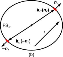
Figure 1: (a) Expansion of the momentum $\bm{p}$ close to the Fermi surface $\mathcal{FS}_{\sigma}$: $\bm{k}_{\sigma}$ is the normal projection of $\bm{p}$ on $\mathcal{FS}_{\sigma}$, $\bm{n}(\bm{k}_{\sigma})$ is the outward normal at $\bm{k}_{\sigma}\in\mathcal{FS}_{\sigma}$, $\delta p\ll k_{F}$. (b) Two points $\bm{k}_{\sigma}(\bm{n}_{\bm{r}})$ and $\bm{k}_{\sigma}(-\bm{n}_{\bm{r}})$ on a nearly spherical Fermi surface $\mathcal{FS}_{\sigma}$ where the outward normals are equal to $\bm{n}_{\bm{r}}$ and $-\bm{n}_{\bm{r}}$, respectively. The two red patches on $\mathcal{FS}_{\sigma}$ correspond to the vicinities $U(\pm\bm{n}_{\bm{r}})$ of the points $\bm{k}_{\sigma}(\pm\bm{n}_{\bm{r}})$ which give the leading contribution to the $\tau\gg 1/E_{F}$ and $r\gg\lambda_{F}$ asymptotics of the Green function, see Eq. (18).

III Asymptotics of the free electron Green function

In the following it is most convenient to work with the electron Green function in the space-time representation. In this paper we operate with the statistical (Matsubara) Green function $G_{\sigma}(\tau,\bm{r})$, where $\tau$ is the imaginary time, $\bm{r}$ the $D$-dimensional coordinate vector, and $\sigma=\pm 1$ the band index. In this section we derive the asymptotics of the free electron Green function $G^{(0)}_{\sigma}(\tau,\bm{r})$ at $\tau\gg 1/E_{F}$ and $r\gg\lambda_{F}$, where $\lambda_{F}=2\pi/k_{F}$ is the Fermi wavelength. Similar derivations can be found in Ref. [64] in application to the Fermi surface imaging.

The asymptotics of $G^{(0)}_{\sigma}(\tau,\bm{r})$ at $\tau\gg 1/E_{F}$ and $r\gg\lambda_{F}$ comes from the sector $(\omega,\bm{p})$ close to the Fermi surface:

$$\omega\ll E_{F},\,\,\bm{p}=\bm{k}_{\sigma}+\bm{n}(\bm{k}_{\sigma})\,\delta p,\,\,\delta p\ll k_{F},$$ (10)

where $\bm{k}_{\sigma}\in\mathcal{FS}_{\sigma}$ is a point on the spin-split Fermi surface $\mathcal{FS}_{\sigma}$ with index $\sigma$, $\bm{n}(\bm{k}_{\sigma})$ is the outward normal at this point, $\delta p>0$ ($\delta p<0$) corresponds to empty (occupied) states at zero temperature, see Fig. 1(a). The free electron Green function $G_{\sigma}^{(0)}(i\omega,\bm{p})$ is given by the quasiparticle pole:

$$G_{\sigma}^{(0)}(i\omega,\bm{p})\equiv G_{\sigma}^{(0)}(i\omega,\delta p,\bm{n})=\frac{|\sigma,\bm{n}\rangle\langle\sigma,\bm{n}|}{i\omega-v_{\sigma}(\bm{n})\delta p},$$ (11)

where we shortened $\bm{n}(\bm{k}_{\sigma})$ to $\bm{n}$ here, $|\sigma,\bm{n}\rangle$ is the spinor given by Eq. (5), $v_{\sigma}(\bm{n})$ is the Fermi velocity at $\bm{k}_{\sigma}$. Here we also linearized the dispersion with respect to $\delta p$ because $\delta p\ll k_{F}$. At the same time, the finite curvature of the Fermi surface is important for the asymptotic form of $G^{(0)}_{\sigma}(\tau,\bm{r})$.

The space-time representation of the free electron Green function is given by the Fourier transform:

$$G_{\sigma}^{(0)}(\tau,\bm{r})=\int\limits_{-\infty}^{\infty}\frac{d\omega}{2\pi}\int\frac{d\bm{p}}{(2\pi)^{D}}e^{i(\bm{p}\cdot\bm{r}-\omega\tau)}G_{\sigma}^{(0)}(i\omega,\bm{p}),$$ (12)

where $G_{\sigma}^{(0)}(i\omega,\bm{p})$ is given by Eq. (11) at the infrared sector defined in Eq. (10). We integrate over the Matsubara frequencies because here we consider the case of zero temperature $T=0$. The integral over $\omega$ is elementary:

$$G_{\sigma}^{(0)}(\tau,\delta p,\bm{n})=\int\limits_{-\infty}^{\infty}\frac{d\omega}{2\pi}e^{-i\omega\tau}\frac{|\sigma,\bm{n}\rangle\langle\sigma,\bm{n}|}{i\omega-v_{\sigma}(\bm{n})\delta p}$$

$$\hskip 30.0pt=-{\rm sgn}(\tau)\theta(\delta p\,\tau)e^{-v_{\sigma}(\bm{n})\delta p\,\tau}|\sigma,\bm{n}\rangle\langle\sigma,\bm{n}|,$$ (13)

where ${\rm sgn}(\tau)$ returns the sign of $\tau$, $\theta(z)$ is the Heaviside step function, i.e. $\theta(z)=0$ ($\theta(z)=1$) if $z<0$ ($z>0$).

The integration over $\bm{p}$ is convenient to perform via thin layers located at the distance $\delta p$ from the Fermi surface $\mathcal{FS}_{\sigma}$. As $\delta p\ll k_{F}$, the measure can be approximated as follows:

$$d\bm{p}\approx d\bm{k}_{\sigma}\,d\delta p,\,\,\bm{k}_{\sigma}\in\mathcal{FS}_{\sigma}.$$ (14)

The momentum is expanded via Eq. (10), see also Fig. 1(a), i.e. $\bm{p}=\bm{k}_{\sigma}+\bm{n}(\bm{k}_{\sigma})\,\delta p$, where the normal $\bm{n}(\bm{k}_{\sigma})$ is taken at the point $\bm{k}_{\sigma}\in\mathcal{FS}_{\sigma}$.

Next, we apply the stationary phase method in order to evaluate the integral over $\bm{k}_{\sigma}\in\mathcal{FS}_{\sigma}$. For this, we first find the stationary points where $\bm{k}_{\sigma}\cdot\bm{r}$ reaches its extrema. This happens when $d\bm{k}_{\sigma}\cdot\bm{r}=0$, where $d\bm{k}_{\sigma}$ is an arbitrary element of the tangent space attached to the Fermi surface $\mathcal{FS}_{\sigma}$ at the point $\bm{k}_{\sigma}\in\mathcal{FS}_{\sigma}$. This condition is satisfied at such points $\bm{k}_{\sigma}\in\mathcal{FS}_{\sigma}$ at which the normals $\bm{n}(\bm{k}_{\sigma})$ are collinear with the coordinate vector $\bm{r}$. As the Fermi surfaces are nearly spherical, see Eq. (9), there are exactly two points $\bm{k}_{\sigma}(\pm\bm{n}_{\bm{r}})\in\mathcal{FS}_{\sigma}$ where the outward normals are equal to $\pm\bm{n}_{\bm{r}}$, $\bm{n}_{\bm{r}}=\bm{r}/r$ is the unit vector along $\bm{r}$, see Fig. 1(b). Thus, we find that the integral over $\bm{p}$ yields the sum of two integrals over small vicinities $U(\pm\bm{n}_{\bm{r}})\subset\mathcal{FS}_{\sigma}$ of the points $\bm{k}_{\sigma}(\pm\bm{n}_{\bm{r}})\in\mathcal{FS}_{\sigma}$, see Fig. 1(b):

$$G_{\sigma}^{(0)}(\tau,\bm{r})\approx\int\limits_{\bm{k}_{\sigma}\in U(\bm{n}_{\bm{r}})}\frac{d\bm{k}_{\sigma}}{(2\pi)^{D-1}}e^{i(\bm{k}_{\sigma}-\bm{k}_{\sigma}(\bm{n}_{\bm{r}}))\cdot\bm{r}}\int\limits_{-\infty}^{\infty}\frac{d\delta p}{2\pi}e^{i\delta p\,r}G_{\sigma}^{(0)}(\tau,\delta p,\bm{n}_{\bm{r}})e^{i\bm{k}_{\sigma}(\bm{n}_{\bm{r}})\cdot\bm{r}}$$

$$+\int\limits_{\bm{k}_{\sigma}\in U(-\bm{n}_{\bm{r}})}\frac{d\bm{k}_{\sigma}}{(2\pi)^{D-1}}e^{i(\bm{k}_{\sigma}-\bm{k}_{\sigma}(-\bm{n}_{\bm{r}}))\cdot\bm{r}}\int\limits_{-\infty}^{\infty}\frac{d\delta p}{2\pi}e^{-i\delta p\,r}G_{\sigma}^{(0)}(\tau,\delta p,-\bm{n}_{\bm{r}})e^{i\bm{k}_{\sigma}(-\bm{n}_{\bm{r}})\cdot\bm{r}},\,\,\,\,\bm{n}_{\bm{r}}=\frac{\bm{r}}{r}.$$ (15)

Here $\bm{k}_{\sigma}(\pm\bm{n}_{\bm{r}})$ are the points on $\mathcal{FS}_{\sigma}$ where the outward normals are equal to $\pm\bm{n}_{\bm{r}}$, see Fig. 1(b). The integration over $\delta p$ is extended to the interval $\delta p\in(-\infty,\infty)$ due to quick convergence on the scale $\delta p\sim 1/r\ll k_{F}$. The integrals over $\bm{k}_{\sigma}$ in the vicinities $U(\pm\bm{n}_{\bm{r}})\subset\mathcal{FS}_{\sigma}$ of the points $\bm{k}_{\sigma}(\pm\bm{n}_{\bm{r}})$ are Gaussian and they are convergent due to the finite Gaussian curvature of nearly spherical Fermi surface $\mathcal{FS}_{\sigma}$ at the points $\bm{k}_{\sigma}(\pm\bm{n}_{\bm{r}})$, see Appendix A for more details . The integrals over $\delta p$ yield the one-dimensional Fourier transforms:

$$G_{\sigma}^{(0)}(\tau,x,\bm{n})=\int\limits_{-\infty}^{\infty}\frac{d\delta p}{2\pi}e^{i\delta p\,x}G_{\sigma}^{(0)}(\tau,\delta p,\bm{n})$$

$$=\frac{1}{2\pi}\frac{|\sigma,\bm{n}\rangle\langle\sigma,\bm{n}|}{ix-v_{\sigma}(\bm{n})\tau},$$ (16)

where $\bm{n}$ here is an arbitrary unit vector and $x\in(-\infty,\infty)$ an effective one-dimensional coordinate. Keeping only the linear order in SO splitting, we show in the Appendix A that

$$\bm{k}_{\sigma}(\pm\bm{n}_{\bm{r}})\cdot\bm{r}\approx\pm k_{\sigma}(\pm\bm{n}_{\bm{r}})r,$$ (17)

where $k_{\sigma}(\bm{n})$ is given by Eq. (9) for arbitrary unit vector $\bm{n}$. The Gaussian integrals over $U(\pm\bm{n}_{\bm{r}})$ are proportional to $1/r^{(D-1)/2}$, see Appendix A for the details. Substituting Eqs. (16) and (17) into Eq. (15) and evaluating the Gaussian integrals over $U(\pm\bm{n}_{\bm{r}})$, we find the infrared long-range asymptotics of the free-electron Matsubara Green function:

$$G^{(0)}_{\sigma}(\tau,\bm{r})\approx\left(\frac{1}{\lambda_{F}r}\right)^{\frac{D-1}{2}}\left[\frac{e^{i(k_{\sigma}(\bm{n}_{\bm{r}})r-\vartheta)}}{2\pi}\frac{|\sigma,\bm{n}_{\bm{r}}\rangle\langle\sigma,\bm{n}_{\bm{r}}|}{ir-v_{F}\tau}\right.$$

$$\left.-\frac{e^{-i(k_{\sigma}(-\bm{n}_{\bm{r}})r-\vartheta)}}{2\pi}\frac{|\sigma,-\bm{n}_{\bm{r}}\rangle\langle\sigma,-\bm{n}_{\bm{r}}|}{ir+v_{F}\tau}\right],\,\,\bm{n}_{\bm{r}}=\frac{\bm{r}}{r},$$ (18)

$$\vartheta=\frac{\pi}{4}(D-1),$$ (19)

where $k_{\sigma}(\bm{n})$ is given by Eq. (9) for arbitrary unit vector $\bm{n}$, $\lambda_{F}$ is the Fermi wavelength, $v_{F}=k_{F}/m$ is the Fermi velocity at zero spin splitting, and $\bm{n}_{\bm{r}}=\bm{r}/r$ is the unit vector along $\bm{r}$. Here we stress that Eq. (18) is true only if the SO splitting is small compared to $E_{F}$, see Eq. (2). We also neglected the weak dependence of the Fermi velocity on the spin splitting in the denominators in Eq. (18) because it does not provide any non-analyticities. We see from Eq. (18) that the Green function contains the oscillatory factors that are sensitive to the spin splitting through $k_{\sigma}(\pm\bm{n}_{\bm{r}})$, see Eq. (9). As we will see later, these oscillatory factors are responsible for the non-analytic terms in the thermodynamic potential $\Omega$.

In the Appendix A we generalize this calculation to the case of a strongly interacting electron gas with a singularity (not necessarily a pole) at the Fermi surface of arbitrary geometry. The Appendix A also contains details for nearly spherical Fermi surfaces. The case of spherical Fermi surfaces is covered in Ref. [58].

IV Non-analyticities in $\Omega$: limit of weak interaction

In this section we calculate the non-analytic corrections to the thermodynamic potential $\Omega$ in the limit of weak electron-electron interaction. The calculation is performed within second order perturbation theory and it is valid in the paramagnetic Fermi liquid phase far away from the FQPT. However, this calculation is important because it allows us to identify the resonant scattering processes close to the Fermi surface which are responsible for the non-analytic terms in $\Omega$. In the following sections we treat these processes non-perturbatively and find that the non-analytic terms are strongly enhanced close to the FQPT. The results of this section extend existing theories [32, 33, 34, 43, 55] to the case of arbitrary spin splitting. In particular, we show that arbitrary SO splitting is not able to gap out all soft fluctuation modes and the non-analyticity in $\Omega$ with respect to the magnetic field $\bm{B}$ survives, in contrast to predictions of Ref. [57]. In this section we are only after the non-analytic terms in $\Omega$, all analytic corrections will be dropped.

Figure 2: (a) First-order interaction correction to $\Omega$, see Eq. (20). (b) Second-order interaction correction to $\Omega$ contributing to the non-analyticity. Solid lines correspond to the electron propagators $G_{\sigma}^{(0)}(\tau,\bm{r})$, see Eq. (18); wiggly lines stand for the Coulomb interaction, see Eq. (22).

IV.1 First-order interaction correction to $\Omega$

Let us start from the first-order interaction correction to $\Omega$, see Fig. 2(a):

$$\Omega^{(1)}=\frac{1}{2}\sum\limits_{\sigma,\sigma^{\prime}}\int dz\,V_{0}(z)P_{\sigma\sigma^{\prime}}(z),$$ (20)

$$P_{\sigma\sigma^{\prime}}(z)=-{\rm Tr}\left\{G^{(0)}_{\sigma}(z)G^{(0)}_{\sigma^{\prime}}(-z)\right\},$$ (21)

where $z=(\tau,\bm{r})$, ${\rm Tr}$ stands for the spin trace, and $P_{\sigma\sigma^{\prime}}(z)$ is the particle-hole bubble. Here, $V_{0}(z)$ is the Coulomb interaction,

$$V_{0}(\tau,\bm{r})=\frac{e^{2}}{\epsilon r}\delta(\tau),$$ (22)

where $e$ is the elementary charge, $\epsilon$ the dielectric constant, and $\delta(\tau)$ is due to the instantaneous nature of the Coulomb interaction (the speed of light is much larger than the Fermi velocity). Using the asymptotics of the Green function $G^{(0)}_{\sigma}(\tau,\bm{r})$, see Eq. (18), we find the asymptotics of the particle-hole bubble:

$$P_{\sigma\sigma^{\prime}}(\tau,\bm{r})=P^{L}_{\sigma\sigma^{\prime}}(\tau,\bm{r})+P^{K}_{\sigma\sigma^{\prime}}(\tau,\bm{r}),$$ (23)

$$P^{L}_{\sigma\sigma^{\prime}}(\tau,\bm{r})\approx\frac{\delta_{\sigma\sigma^{\prime}}}{2\pi^{2}}\left(\frac{1}{\lambda_{F}r}\right)^{D-1}\frac{v_{F}^{2}\tau^{2}-r^{2}}{(r^{2}+v_{F}^{2}\tau^{2})^{2}},$$ (24)

$$P^{K}_{\sigma\sigma^{\prime}}(\tau,\bm{r})\approx\frac{1}{4\pi^{2}}\frac{1}{r^{2}+v_{F}^{2}\tau^{2}}\left(\frac{1}{\lambda_{F}r}\right)^{D-1}$$

$$\times\left[e^{-2i\vartheta}e^{ir(k_{\sigma}(\bm{n}_{\bm{r}})+k_{\sigma^{\prime}}(-\bm{n}_{\bm{r}}))}\left|M_{\sigma\sigma^{\prime}}(\bm{n}_{\bm{r}})\right|^{2}\right.$$

$$\left.+e^{2i\vartheta}e^{-ir(k_{\sigma}(-\bm{n}_{\bm{r}})+k_{\sigma^{\prime}}(\bm{n}_{\bm{r}}))}\left|M_{\sigma\sigma^{\prime}}(-\bm{n}_{\bm{r}})\right|^{2}\right],$$ (25)

where the matrix elements $M_{\sigma\sigma^{\prime}}(\pm\bm{n}_{\bm{r}})$ are given by Eq. (8). Here $P^{L}_{\sigma\sigma^{\prime}}(\tau,\bm{r})$ is the Landau damping contribution to the particle-hole bubble coming from the forward scattering. It is clear that this contribution is insensitive to the spin splitting. The second contribution, $P^{K}_{\sigma\sigma^{\prime}}(\tau,\bm{r})$, is the Kohn anomaly coming from the backscattering with the momentum transfer close to $2k_{F}$. The Kohn anomaly is sensitive to the spin splitting through the oscillatory factors containing the Fermi momenta $k_{\sigma}(\pm\bm{n}_{\bm{r}})$, see Eq. (9).

As only the Kohn anomaly is sensitive to the spin splitting $\mbox{\boldmath{$\beta$}}(\bm{n}_{\bm{p}})$, we can simplify Eq. (20):

$$\Omega^{(1)}=\frac{1}{2}\sum\limits_{\sigma,\sigma^{\prime}}\int\limits_{S_{D-1}}d\bm{n}_{\bm{r}}\int\limits_{0}^{\infty}dr\,r^{D-1}\frac{e^{2}}{\epsilon r}P^{K}_{\sigma\sigma^{\prime}}(0,\bm{r}),$$ (26)

where $S_{D-1}$ is the $(D-1)$-dimensional unit sphere, $d\bm{r}=r^{D-1}\,dr\,d\bm{n}_{\bm{r}}$. The integral over $r$ is divergent at small $r$ (the ultraviolet divergence) because it takes the following form:

$$\int\limits_{0}^{\infty}\frac{dr}{r^{3}}e^{ir\Delta}\to\infty,$$ (27)

where $\Delta$ is either equal to $\Delta=k_{\sigma}(\bm{n}_{\bm{r}})+k_{\sigma^{\prime}}(-\bm{n}_{\bm{r}})$ or to $\Delta=-k_{\sigma}(-\bm{n}_{\bm{r}})-k_{\sigma^{\prime}}(\bm{n}_{\bm{r}})$. This divergence comes from the asymptotics of the particle-hole bubble, see Eq. (25), that is only valid at $r\gg\lambda_{F}$. Therefore, the lower limit for $r$ in Eq. (27) is bounded by $r\sim\lambda_{F}$. This divergence can also be cured via the analytical continuation to the Euler gamma function $\Gamma(x)$ using the following identity:

$$I_{\alpha}(\Delta)=\int\limits_{0}^{\infty}\frac{dr}{r^{\alpha}}e^{ir\Delta}=\frac{\pi|\Delta|^{\alpha-1}}{\sin(\pi\alpha)\Gamma(\alpha)}e^{-i\frac{\pi}{2}(\alpha-1){\rm sgn}(\Delta)}.$$ (28)

In our case $\alpha=3$ and the integral is indeed divergent due to $\sin(3\pi)=0$ in the denominator. Therefore, we consider $\alpha=3+\delta$ and take the limit $\delta\to 0$:

$$\int\limits_{0}^{\infty}\frac{dr}{r^{3}}e^{ir\Delta}=\frac{\Delta^{2}}{2}\left(\frac{1}{\delta}+\ln\left|\Delta\right|-i\frac{\pi}{2}{\rm sgn}\left(\Delta\right)\right).$$ (29)

Now it is clear that the physical dimension of $\Delta$ under the logarithm has to be compensated by the ultraviolet scale $p_{0}\sim 2k_{F}$ which is equivalent to cutting the lower limit in Eq. (27) at $r\sim\lambda_{F}$:

$$\int\limits_{\sim\lambda_{F}}^{\infty}\frac{dr}{r^{3}}e^{ir\Delta}=\frac{\Delta^{2}}{2}\left(\ln\left|\frac{\Delta}{p_{0}}\right|-i\frac{\pi}{2}{\rm sgn}\left(\Delta\right)\right).$$ (30)

Now, we come back to $\Omega^{(1)}$ where $\Delta$ is either equal to $\Delta=k_{\sigma}(\bm{n}_{\bm{r}})+k_{\sigma^{\prime}}(-\bm{n}_{\bm{r}})$ or to $\Delta=-k_{\sigma}(-\bm{n}_{\bm{r}})-k_{\sigma^{\prime}}(\bm{n}_{\bm{r}})$, so using Eq. (9) we find:

$$|\Delta|\approx 2k_{F}+\frac{\sigma\beta(\pm\bm{n}_{\bm{r}})+\sigma^{\prime}\beta(\mp\bm{n}_{\bm{r}})}{v_{F}}.$$ (31)

As the spin splitting is much smaller than the Fermi energy, we can expand the logarithm $\ln|\Delta/p_{0}|$ in the analytic Taylor series with respect to the spin splitting. Hence, we see that $\Omega^{(1)}$ does not contain any non-analyticities for arbitrary spin splitting.

Here we have performed the calculations for the long-range Coulomb interaction Eq. (22). Finite electron density results in the Thomas-Fermi screening of the long range Coulomb tail on the scale of the screening length $r_{0}$. The weak coupling limit that we consider in this section corresponds to $r_{0}\gg\lambda_{F}$. However, the integral over $r$ in $\Omega^{(1)}$ converges at $r\sim\lambda_{F}\ll r_{0}$, because $\Delta\approx 2k_{F}$ here. Therefore, we can indeed neglect the Thomas-Fermi screening in this section.

Figure 3: Other second-order diagrams that do not contribute to the non-analyticities in $\Omega$, see Eqs. (45), (46).

IV.2 Second-order interaction corrections to $\Omega$

We see from the calculation of $\Omega^{(1)}$ that the non-analytic terms may come from the oscillatory integrals like the one in Eq. (28). However, we have to subtract the $2k_{F}$ factor first, such that $\Delta$ in Eq. (28) becomes proportional to the spin splitting. One way to achieve this is to consider $\Omega^{(1)}$, see Eq. (20), with the interaction $V(\tau,\bm{r})$ which has oscillatory components $e^{\pm i2k_{F}r}$. In fact, the electron-electron interaction acquires such components upon the dynamic screening by the particle-hole bubble. One consequence of this is the Thomas-Fermi screening which we already discussed and concluded that it is not important if the interaction is weak. However, there is another much more important consequence of such dressing that results in $2k_{F}$ harmonics in the interaction due to backscattering of electrons near the Fermi surface, the effect known as Friedel oscillations. As we consider the correlations at large $r\sim v_{F}/\beta\gg\lambda_{F}$, where $\beta$ is a characteristic value of the spin splitting at the Fermi surface, the interaction matrix elements at the momentum transfer $2k_{F}$ are effectively local, so we can use the effective contact interaction:

$$V_{2k_{F}}(z)=u\,\delta(\bm{r})\delta(\tau)=u\,\delta(z),$$ (32)

$$u\approx V_{0}(2k_{F})=\frac{2\pi^{\frac{D}{2}}\Gamma(D-1)}{\Gamma\left(\frac{D}{2}\right)}\frac{e^{2}}{\epsilon(2k_{F})^{D-1}},$$ (33)

where $\delta(\bm{r})$ is the $D$-dimensional delta function, $V_{0}(q)$ is the Fourier transform of the Coulomb interaction Eq. (22).

If we dress the interaction line in Fig. 2(a) by a single particle-hole bubble, we get the second-order diagram for $\Omega$ shown in Fig. 2(b):

$$\Omega^{(2)}=-\frac{1}{4}\sum\limits_{\sigma_{i}}\int dz_{1}dz_{2}dz_{3}\,V_{2k_{F}}(z_{2})V_{2k_{F}}(z_{3}-z_{1})$$

$$\hskip 70.0pt\times P_{\sigma_{1}\sigma_{2}}(z_{1})P_{\sigma_{3}\sigma_{4}}(z_{3}-z_{2}).$$ (34)

Using the contact approximation Eq. (32), we simplify $\Omega^{(2)}$ to the following expression:

$$\Omega^{(2)}=-\frac{u^{2}}{4}\sum\limits_{\sigma_{i}}\int dz\,P_{\sigma_{1}\sigma_{2}}(z)P_{\sigma_{3}\sigma_{4}}(z),$$ (35)

where $z=(\tau,\bm{r})$. From Eqs. (23)–(25) we find that only the product of Kohn anomalies contains slowly oscillating terms on the scale $v_{F}/\beta$, where $\beta$ stands for the characteristic spin splitting at the Fermi surface:

$$P_{\sigma_{1}\sigma_{2}}(z)P_{\sigma_{3}\sigma_{4}}(z)=\frac{e^{ir\Delta^{\sigma_{1}\sigma_{2}}_{\sigma_{3}\sigma_{4}}(\bm{n}_{\bm{r}})}\left|M_{\sigma_{1}\sigma_{2}}(\bm{n}_{\bm{r}})M_{\sigma_{3}\sigma_{4}}(-\bm{n}_{\bm{r}})\right|^{2}+e^{-ir\Delta^{\sigma_{1}\sigma_{2}}_{\sigma_{3}\sigma_{4}}(-\bm{n}_{\bm{r}})}\left|M_{\sigma_{1}\sigma_{2}}(-\bm{n}_{\bm{r}})M_{\sigma_{3}\sigma_{4}}(\bm{n}_{\bm{r}})\right|^{2}}{\left(2\pi\right)^{4}\left(\lambda_{F}r\right)^{2(D-1)}\left(r^{2}+v_{F}^{2}\tau^{2}\right)^{2}}+\dots,$$ (36)

$$\Delta^{\sigma_{1}\sigma_{2}}_{\sigma_{3}\sigma_{4}}(\bm{n}_{\bm{r}})=k_{\sigma_{1}}(\bm{n}_{\bm{r}})+k_{\sigma_{2}}(-\bm{n}_{\bm{r}})-k_{\sigma_{3}}(-\bm{n}_{\bm{r}})-k_{\sigma_{4}}(\bm{n}_{\bm{r}})\approx\frac{\left(\sigma_{1}-\sigma_{4}\right)\beta(\bm{n}_{\bm{r}})+\left(\sigma_{2}-\sigma_{3}\right)\beta(-\bm{n}_{\bm{r}})}{v_{F}},$$ (37)

where dots in Eq. (36) stand for the rapidly oscillating terms on the scale of $2k_{F}$ and $4k_{F}$ and also the forward scattering contribution which does not contain any non-analytic dependence on the spin splitting. We used Eq. (9) to express $\Delta^{\sigma_{1}\sigma_{2}}_{\sigma_{3}\sigma_{4}}(\bm{n}_{\bm{r}})$ in terms of the spin splitting.

Then we substitute Eq. (36) into Eq. (35) and evaluate the integral over $z=(\tau,\bm{r})$. The integral over $\tau$ is elementary:

$$\int\limits_{-\infty}^{\infty}\frac{d\tau}{\left(r^{2}+v_{F}^{2}\tau^{2}\right)^{2}}=\frac{\pi}{2v_{F}r^{3}}.$$ (38)

The integral over $r$ can be represented using the integral $I_{\alpha}(\Delta)$ defined in Eq. (28):

$$\Omega^{(2)}=-\frac{u^{2}}{2^{6}\pi^{3}v_{F}\lambda_{F}^{2(D-1)}}\sum\limits_{\sigma_{i}}\int\limits_{S_{D-1}}d\bm{n}_{\bm{r}}$$

$$\left|M_{\sigma_{1}\sigma_{2}}(\bm{n}_{\bm{r}})M_{\sigma_{3}\sigma_{4}}(-\bm{n}_{\bm{r}})\right|^{2}{\rm Re}\left(I_{D+2}\left(\Delta^{\sigma_{1}\sigma_{2}}_{\sigma_{3}\sigma_{4}}(\bm{n}_{\bm{r}})\right)\right),$$ (39)

where ${\rm Re}$ stands for the real part. Here we used that $I_{\alpha}(-x)=I^{*}_{\alpha}(x)$, where the star corresponds to the complex conjugation.

At this point it is convenient to introduce the dimensionless interaction parameter $g$:

$$g=uN_{F}=\frac{umk_{F}^{D-2}}{2^{D-1}\pi^{\frac{D}{2}}\Gamma\left(\frac{D}{2}\right)},$$ (40)

where $N_{F}$ is the density of states per band at the Fermi level. Substituting Eq. (33) into Eq. (40), we find an estimate for the dimensionless coupling constant $g$:

$$g\approx\frac{\Gamma(D-1)}{2^{2D-3}\Gamma^{2}\left(\frac{D}{2}\right)}\frac{1}{k_{F}a_{B}},\,\,a_{B}=\frac{\epsilon}{me^{2}},$$ (41)

where $a_{B}$ is the effective Bohr radius. The weak coupling regime corresponds to high densities such that $k_{F}a_{B}\gg 1$ or $g\ll 1$.

Then Eq. (39) can be represented in the following form:

$$\Omega^{(2)}=L_{D}\frac{v_{F}^{D+1}}{2^{D+2}}\sum\limits_{\sigma_{i}}\int\limits_{S_{D-1}}d\bm{n}_{\bm{r}}\,$$

$$\hskip 10.0pt\times\left|M_{\sigma_{1}\sigma_{2}}(\bm{n}_{\bm{r}})M_{\sigma_{3}\sigma_{4}}(-\bm{n}_{\bm{r}})\right|^{2}\left|\Delta^{\sigma_{1}\sigma_{2}}_{\sigma_{3}\sigma_{4}}(\bm{n}_{\bm{r}})\right|^{D+1},$$ (42)

$$L_{D}=\frac{g^{2}}{32}\left(\frac{2}{\pi v_{F}}\right)^{D}\frac{\Gamma^{2}\left(\frac{D}{2}\right)}{\Gamma\left(D+2\right)}\frac{1}{\cos\left(\pi\frac{D}{2}\right)}.$$ (43)

We perform the summation over the band indexes $\sigma_{i}$ explicitly:

$$\Omega^{(2)}=L_{D}\int\limits_{S_{D-1}}d\bm{n}\left[\left|M_{+-}(\bm{n})M_{+-}(-\bm{n})\right|^{2}\left|\beta(\bm{n})-\beta(-\bm{n})\right|^{D+1}+\left|M_{++}(\bm{n})M_{--}(\bm{n})\right|^{2}\left|\beta(\bm{n})+\beta(-\bm{n})\right|^{D+1}\right.$$

$$\hskip 140.0pt\left.+2\left(\left|M_{++}(\bm{n})M_{-+}(\bm{n})\right|^{2}+\left|M_{--}(\bm{n})M_{+-}(\bm{n})\right|^{2}\right)\left|\beta(\bm{n})\right|^{D+1}\right].$$ (44)

Here we dropped the index $\bm{r}$ in $\bm{n}_{\bm{r}}$, such that $\bm{n}$ can be also interpreted as the unit vector $\bm{n}_{\bm{p}}=\bm{p}/p$, $p\approx k_{F}$, in the momentum space. This interpretation makes sense because the asymptotics of the Green function, see Eq. (18), comes from small vicinities of two points on the Fermi surface whose outward normals are collinear with $\bm{r}$. So, $\bm{r}$ and $\bm{p}$ are in a way pinned to each other.

Finally, we have to check that the second-order diagrams in Fig. 3(a),(b) do not contribute to the non-analytic terms in $\Omega$:

$$\Omega_{a}=\frac{u^{2}}{2}\sum\limits_{\sigma_{i}}\int dz\,$$

$$\hskip 30.0pt{\rm Tr}\left\{G_{\sigma_{1}}^{(0)}(0)G_{\sigma_{2}}^{(0)}(z)G_{\sigma_{3}}^{(0)}(0)G_{\sigma_{4}}^{(0)}(-z)\right\},$$ (45)

$$\Omega_{b}=\frac{u^{2}}{4}\sum\limits_{\sigma_{i}}\int dz\,$$

$$\hskip 30.0pt{\rm Tr}\left\{G_{\sigma_{1}}^{(0)}(z)G_{\sigma_{2}}^{(0)}(-z)G_{\sigma_{3}}^{(0)}(z)G_{\sigma_{4}}^{(0)}(-z)\right\}.$$ (46)

Here $G_{\sigma}^{(0)}(0)=G_{\sigma}^{(0)}(\tau=-0,\bm{r}=0)$ due to the ordering of the field operators within the interaction Hamiltonian:

$$G_{\sigma}^{(0)}(0)=\int\frac{d\bm{p}}{(2\pi)^{D}}\theta(k_{\sigma}(\bm{n}_{\bm{p}})-p)|\sigma,\bm{n}_{\bm{p}}\rangle\langle\sigma,\bm{n}_{\bm{p}}|,$$ (47)

where $|\sigma,\bm{n}_{\bm{p}}\rangle$ are the eigenvectors of the single-particle Hamiltonian, see Eq. (5), and $k_{\sigma}(\bm{n}_{\bm{p}})$ is given by Eq. (9).

The diagram $\Omega_{a}$ has a single particle-hole bubble in it due to the Green functions $G_{\sigma_{2}}^{(0)}(z)$ and $G_{\sigma_{4}}^{(0)}(-z)$, see Eq. (45). The product of these Green functions contains weakly oscillating terms and $\approx 2k_{F}$ harmonics. As in the case of $\Omega^{(1)}$, the $2k_{F}$ harmonics do not produce any non-analyticities. The weakly oscillating terms originate from the Landau damping part of the particle-hole bubble but these terms vanish due to the integral over $\tau$:

$$\int\limits_{-\infty}^{\infty}\frac{d\tau}{(v_{F}\tau\pm ir)^{2}}=0.$$ (48)

The diagram $\Omega_{b}$ is more complicated. Let us consider two matrix products $G_{\sigma_{1}}^{(0)}(z)G_{\sigma_{2}}^{(0)}(-z)$ and $G_{\sigma_{3}}^{(0)}(z)G_{\sigma_{4}}^{(0)}(-z)$, spin traces are not taken here. As usual, we are after the slowly oscillating terms in Eq. (46). One possibility for this is the product of the forward scattering contributions coming from $G_{\sigma_{1}}^{(0)}(z)G_{\sigma_{2}}^{(0)}(-z)$ and $G_{\sigma_{3}}^{(0)}(z)G_{\sigma_{4}}^{(0)}(-z)$. From Eq. (18) it is clear that the forward scattering contributions are non-zero only if $\sigma_{1}=\sigma_{2}$ and $\sigma_{3}=\sigma_{4}$, matrix products of corresponding projectors vanish otherwise. However, in this case the oscillating factors are canceled exactly and thus, this contribution is analytic. Another way to obtain slowly oscillating terms in Eq. (46) is the product of Kohn anomalies contained in $G_{\sigma_{1}}^{(0)}(z)G_{\sigma_{2}}^{(0)}(-z)$ and $G_{\sigma_{3}}^{(0)}(z)G_{\sigma_{4}}^{(0)}(-z)$. In this case, we have to look at the spin trace in Eq. (46) which is non-zero only if $\sigma_{1}=\sigma_{4}$ and $\sigma_{2}=\sigma_{3}$. This condition becomes obvious if we notice that the product of Kohn anomalies of $G_{\sigma_{1}}^{(0)}(z)G_{\sigma_{2}}^{(0)}(-z)$ and $G_{\sigma_{3}}^{(0)}(z)G_{\sigma_{4}}^{(0)}(-z)$ is actually equivalent to the product of the forward scattering contributions of $G_{\sigma_{2}}^{(0)}(-z)G_{\sigma_{3}}^{(0)}(z)$ and $G_{\sigma_{4}}^{(0)}(-z)G_{\sigma_{1}}^{(0)}(z)$ which is analytic for the reasons we discussed above.

Hence, only the diagram in Fig. 2(b) contains non-analytic terms and, therefore, Eq. (44) describes the non-analytic corrections to $\Omega$ due to arbitrary spin splitting $\mbox{\boldmath{$\beta$}}(\bm{p})$ within second-order perturbation theory.

Even though Eq. (44) is true in arbitrary number $D$ of spatial dimensions, we give explicit expressions for $D=2$ and $D=3$. For 2DEG the coefficient $L_{2}$ is negative, see Eq. (43) for $D=2$:

$$L_{2}=-\frac{g^{2}}{48\pi^{2}v_{F}^{2}}.$$ (49)

The integral over $d\bm{n}$ can be parametrized by a single angle $\phi\in(0,2\pi]$, so the non-analytic correction Eq. (44) for 2DEG then reads:

$$\Omega^{(2)}=-\frac{g^{2}}{24\pi v_{F}^{2}}\int\limits_{0}^{2\pi}\frac{d\phi}{2\pi}\left[\left|M_{+-}(\phi)M_{-+}(\phi)\right|^{2}\left|\beta(\phi)-\beta(\phi+\pi)\right|^{3}+\left|M_{++}(\phi)M_{--}(\phi)\right|^{2}\left|\beta(\phi)+\beta(\phi+\pi)\right|^{3}\right.$$

$$\hskip 95.0pt\left.+2\left(\left|M_{++}(\phi)M_{-+}(\phi)\right|^{2}+\left|M_{--}(\phi)M_{+-}(\phi)\right|^{2}\right)\left|\beta(\phi)\right|^{3}\right],\,\,\,\,D=2.$$ (50)

Our result Eq. (50) agrees with previous studies [55, 56, 43] and extends them to the case of arbitrary spin splitting. Equation (50) together with Eq. (8) for the matrix elements allows one to find the non-analytic terms in $\Omega$ directly from the spin splitting $\mbox{\boldmath{$\beta$}}(\bm{n})$.

The case of $D=3$ is marginal because the non-analytic terms in Eq. (44) are proportional to the fourth power of the spin splitting. The non-analyticity itself comes from the divergence of the $L_{D}$ prefactor at $D=3$, see Eq. (43), which results in an additional logarithm. This is best seen from the dimensional regularization:

$$D=3-\delta,\,\,\delta\to+0.$$ (51)

The dimension $D$ enters Eq. (44) in the following form:

$$L_{D}\Delta^{D+1}=-\frac{g^{2}\Delta^{4}}{192\pi^{3}v_{F}^{3}}\left(\frac{1}{\delta}-\ln\Delta\right)+\mathcal{O}(\delta),$$ (52)

where $\Delta$ takes one of the following values: $\Delta=|\beta(\bm{n})\pm\beta(-\bm{n})|$ or $\Delta=|\beta(\bm{n})|$. Here we expanded the expression at $\delta\to+0$. The divergent $1/\delta$ contribution is actually analytic and can be represented by $\ln\Lambda$ factor, $\Lambda\sim E_{F}$, which compensates the physical dimension of $\Delta$:

$$L_{D}\Delta^{D+1}\to\frac{g^{2}}{48\pi^{2}v_{F}^{3}}\frac{\Delta^{4}}{4\pi}\ln\left|\frac{\Delta}{\Lambda}\right|,\,\,\Lambda\sim E_{F}.$$ (53)

Using the regularization Eq. (53), we find the non-analytic correction to the spin-split 3DEG:

$$\Omega^{(2)}=\frac{g^{2}}{48\pi^{2}v_{F}^{3}}\int\limits_{S_{2}}\frac{d\bm{n}}{4\pi}\left[\left|M_{+-}(\bm{n})M_{-+}(\bm{n})\right|^{2}\left|\beta(\bm{n})-\beta(-\bm{n})\right|^{4}\ln\left|\frac{\beta(\bm{n})-\beta(-\bm{n})}{\Lambda}\right|\right.$$

$$+\left|M_{++}(\bm{n})M_{--}(\bm{n})\right|^{2}\left|\beta(\bm{n})+\beta(-\bm{n})\right|^{4}\ln\left|\frac{\beta(\bm{n})+\beta(-\bm{n})}{\Lambda}\right|$$

$$\left.+2\left(\left|M_{++}(\bm{n})M_{-+}(\bm{n})\right|^{2}+\left|M_{--}(\bm{n})M_{+-}(\bm{n})\right|^{2}\right)\left|\beta(\bm{n})\right|^{4}\ln\left|\frac{\beta(\bm{n})}{\Lambda}\right|\right],\,\,\,\,\Lambda\sim E_{F},\,\,\,\,D=3.$$ (54)

Here, integration over the unit sphere $S_{2}$ means $d\bm{n}=\sin\phi_{1}\,d\phi_{1}d\phi_{2}$, $\phi_{1}\in[0,\pi]$, $\phi_{2}\in(0,2\pi]$. The non-analytic correction is negatively defined for arbitrary spin splitting due to the logarithms. In particular, if $\mbox{\boldmath{$\beta$}}(\bm{n})=\bm{B}$, we get the well-known result, see Ref. [43]:

$$\Omega^{(2)}=\frac{g^{2}B^{4}}{3\pi^{2}v_{F}^{3}}\ln\left|\frac{2B}{\Lambda}\right|,\,\,\Lambda\sim E_{F}.$$ (55)

IV.3 Large SO splitting and small magnetic field

Here, we consider the important special case of arbitrary SO splitting and small magnetic field:

$$\mbox{\boldmath{$\beta$}}(\bm{n}_{\bm{p}})=\mbox{\boldmath{$\beta$}}_{SO}(\bm{n}_{\bm{p}})+\bm{B},\,\,B\ll\beta_{SO},$$ (56)

where $\bm{n}_{\bm{p}}=\bm{p}/p$, $p\approx k_{F}$, $\beta_{SO}$ is a characteristic value of the SO splitting at the Fermi surface. As any SO splitting respects time reversal symmetry, it has to be an odd vector function of $\bm{n}_{\bm{p}}$:

$$\mbox{\boldmath{$\beta$}}_{SO}(-\bm{n}_{\bm{p}})=-\mbox{\boldmath{$\beta$}}_{SO}(\bm{n}_{\bm{p}}).$$ (57)

As we consider $B\ll\beta_{SO}$, then we can expand $\beta(\bm{n})$ with respect to $\bm{B}$:

$$\beta(\bm{n})\approx\beta_{SO}(\bm{n})+\frac{\mbox{\boldmath{$\beta$}}_{SO}(\bm{n})\cdot\bm{B}}{\beta_{SO}(\bm{n})},$$ (58)

where $\beta_{SO}(\bm{n})=|\mbox{\boldmath{$\beta$}}_{SO}(\bm{n})|$. Together with the symmetry condition Eq. (57), we conclude that only the very first term in Eq. (44) contributes to the non-analyticity with respect to $\bm{B}$ due to the following identity:

$$\beta(\bm{n})-\beta(-\bm{n})\approx 2\frac{\mbox{\boldmath{$\beta$}}_{SO}(\bm{n})\cdot\bm{B}}{\beta_{SO}(\bm{n})}.$$ (59)

As we only consider the leading non-analyticity, we calculate the matrix elements at $\bm{B}=0$:

$$M_{\sigma\sigma}(\bm{n})=0,\,\,M_{\sigma-\sigma}(\bm{n})=-1.$$ (60)

Substituting Eqs. (59), (60) in Eq. (44), we find the non-analytic in $\bm{B}$ correction to $\Omega$ in case of arbitrary SO splitting:

$$\delta\Omega(\bm{B})=L_{D}\int\limits_{S_{D-1}}d\bm{n}\,\left|2\frac{\mbox{\boldmath{$\beta$}}_{SO}(\bm{n})\cdot\bm{B}}{\beta_{SO}(\bm{n})}\right|^{D+1},$$ (61)

where $\delta\Omega(\bm{B})$ indicates that only the non-analytic terms with respect to $\bm{B}$ are included. Thus, we see that the non-analyticity in magnetic field $\bm{B}$ cannot be eliminated even by arbitrary SO splitting, in contrast to the predictions of Ref. [57].

The elementary processes that are responsible for the non-analyticity given by Eq. (61) are shown in Fig. 4. These processes describe the resonant scattering of a pair of electrons with the band index $\sigma$ and opposite momenta $\pm\bm{k}_{\sigma}$ into a pair of electrons in the other band with index $-\sigma$ and momenta $\pm\bm{k}_{-\sigma}$ that are collinear with momenta of initial electrons $\pm\bm{k}_{\sigma}$. The momentum transfer in such a scattering processes is close to $2k_{F}$, see Fig. 4(b). The scattering with small momentum transfer is forbidden due to the orthogonality condition Eq. (6). The considered processes are resonant due to the time reversal symmetry, see Eq. (57). The collinearity condition comes from the local nesting when the momentum transfer between the resonantly scattering states also matches small vicinities around these states. This matching is satisfied when the outward normals in the scattering states are collinear such that the mismatch comes only from different curvatures of the Fermi surface in the considered points. The local nesting strongly enhances corresponding scattering processes because not only the considered states are in resonance but also small vicinities of states around them. For example, the Kohn anomaly in the particle-hole bubble is a result of such a local nesting for the states scattering with the $2k_{F}$ momentum transfer. The perfect local nesting corresponds to the Landau damping of the particle-hole excitations with energy and momentum around zero, in this case the scattered region in the particle-hole bubble is mapped onto itself.

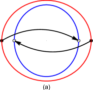
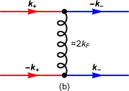
Figure 4: (a) Fermi surfaces at arbitrary SO splitting, red (blue) color corresponds to $\sigma=+1$ ($\sigma=-1$). The arrows show the resonant scattering processes. (b) The interaction matrix element corresponding to the resonant scattering processes at finite SO splitting. Here a pair of electrons with the band index $\sigma=+1$ and opposite momenta $\pm\bm{k}_{+}$ scatter into a pair with momenta $\pm\bm{k}_{-}$ that are collinear with $\pm\bm{k}_{+}$. These processes are resonant due to the time reversal symmetry, see Eq. (57). The collinearity of $\bm{k}_{+}$ and $\bm{k}_{-}$ is due to the local nesting discussed in the main text after Eq. (61). These processes are responsible for the non-analyticity in $\Omega$ with respect to small magnetic field $\bm{B}$, see Eq. (61).

It is also instructive to write down Eq. (61) for 2DEG and 3DEG explicitly:

$$\delta\Omega(\bm{B})=-\frac{g^{2}|B|^{3}}{3\pi v_{F}^{2}}\int\limits_{0}^{2\pi}\frac{d\phi}{2\pi}\left|\frac{\mbox{\boldmath{$\beta$}}_{SO}(\phi)\cdot\bm{b}}{\beta_{SO}(\phi)}\right|^{3},\,\,D=2,$$ (62)

$$\delta\Omega(\bm{B})=\frac{g^{2}B^{4}}{3\pi^{2}v_{F}^{3}}\ln\left|\frac{2B}{\Lambda}\right|$$

$$\hskip 70.0pt\times\int\limits_{S_{2}}\frac{d\bm{n}}{4\pi}\left|\frac{\mbox{\boldmath{$\beta$}}_{SO}(\bm{n})\cdot\bm{b}}{\beta_{SO}(\bm{n})}\right|^{4},\,\,D=3,$$ (63)

where $\bm{b}=\bm{B}/B$ is the unit vector along $\bm{B}$. We neglected the term $\ln|\mbox{\boldmath{$\beta$}}_{SO}(\bm{n})\cdot\bm{b}/\beta_{SO}(\bm{n})|$ in Eq. (63) because it just slightly renormalizes the regular $B^{4}$ term. Here it is convenient to introduce the angular form-factor $F_{D}(\bm{b})$ which depends on the direction $\bm{b}$ of the magnetic field and on the SO splitting:

$$F_{D}(\bm{b})=\int\limits_{S_{D-1}}\frac{d\bm{n}}{S_{D-1}}\left|\frac{\mbox{\boldmath{$\beta$}}_{SO}(\bm{n})\cdot\bm{b}}{\beta_{SO}(\bm{n})}\right|^{D+1},$$ (64)

where $S_{D-1}$ is the area of a unit $(D-1)$-dimensional sphere.

The form-factors $F_{D}(\bm{b})$ can only be positive or zero, see Eq. (64). If we demand $F_{D}(\bm{b})=0$ for any unit vector $\bm{b}$, it is equivalent to say that $\mbox{\boldmath{$\beta$}}_{SO}(\bm{n})\cdot\bm{b}=0$ for any $\bm{b}$ and also $\beta_{SO}(\bm{n})\neq 0$ from Eq. (56). As this is clearly impossible, we conclude that $F_{D}(\bm{b})$ can never vanish for all unit vectors $\bm{b}$ even at arbitrary SO splitting $\mbox{\boldmath{$\beta$}}_{SO}(\bm{n})$. Therefore, the non-analyticity with respect to $\bm{B}$ cannot be cut by any SO splitting neither in 2DEG nor in 3DEG.

Nevertheless, the SO splitting is important because it leads to strong anisotropy of the non-analytic term, see Eq. (61), which is described by the form-factor $F_{D}(\bm{b})$. If we extrapolate this result to the vicinity of a FQPT, we conclude that the direction of spontaneous magnetization must coincide with the maximum of $F_{D}(\bm{b})$. In particular, we predict a first-order Ising FQPT in electron gas with a general SO splitting which breaks the spin rotational symmetry down to $\mathbb{Z}_{2}$.

As an example, we consider a 2DEG with Rashba and Dresselhaus SO splittings:

$$\mbox{\boldmath{$\beta$}}_{SO}(\phi)$$

$$=\left((\alpha_{D}+\alpha_{R})k_{F}\sin\phi,(\alpha_{D}-\alpha_{R})k_{F}\cos\phi,0\right),$$ (65)

where the $x$ and $y$ axes correspond to the $[110]$ and $[1\overline{1}0]$ crystallographic directions, $\alpha_{R}$ and $\alpha_{D}$ are the Rashba and the Dresselhaus coupling constants, respectively. The qualitative picture of the SO-split Fermi surfaces is shown in Fig. 4(a). It is more convenient to introduce the following SO couplings:

$$a_{\pm}\equiv\left(\alpha_{R}\pm\alpha_{D}\right)k_{F}.$$ (66)

Then we find the angular form-factor $F_{2}(\bm{b})$, see Eqs. (62), (64):

$$F_{2}(\bm{b})=\int\limits_{0}^{\pi}\frac{d\phi}{\pi}\frac{\left|a_{+}b_{x}\sin\phi\,-a_{-}b_{y}\cos\phi\,\right|^{3}}{\left(a_{+}^{2}\sin^{2}\phi+a_{-}^{2}\cos^{2}\phi\right)^{\frac{3}{2}}},$$ (67)

where $\bm{b}=\bm{B}/B$ is the unit vector along $\bm{B}$. We want to identify the directions $\bm{b}^{*}$ where $F_{2}(\bm{b}^{*})$ is maximal. It is clear that all such directions have $b^{*}_{z}=0$. Then $b_{x}^{*}$ and $b_{y}^{*}$ can be parametrized by a single angle $\Psi$:

$$b_{x}^{*}=\cos\Psi,\,\,b_{y}^{*}=\sin\Psi.$$ (68)

The integral in Eq. (67) is quite cumbersome but elementary:

$$\frac{2}{3}F_{2}(\zeta,\Psi)=-\frac{\zeta\cos\left(2\Psi\right)}{\zeta^{2}-1}+\frac{\zeta\cos\Psi}{(\zeta^{2}-1)^{\frac{3}{2}}}\left(\zeta^{2}\cos^{2}\Psi-3\sin^{2}\Psi\right)\arctan\left(\sqrt{\zeta^{2}-1}\cos\Psi\right)$$

$$+\frac{\sin\Psi}{(\zeta^{2}-1)^{\frac{3}{2}}}\left(\sin^{2}\Psi-3\zeta^{2}\cos^{2}\Psi\right)\ln\left(\frac{\sqrt{\zeta^{2}\cos^{2}\Psi+\sin^{2}\Psi}}{\sqrt{\zeta^{2}-1}\sin\Psi+\zeta}\right),\,\,\zeta\equiv\left|\frac{a_{+}}{a_{-}}\right|=\left|\frac{\alpha_{R}+\alpha_{D}}{\alpha_{R}-\alpha_{D}}\right|>1.$$ (69)

We added $\zeta$ as additional argument of $F_{2}(\bm{b})$ for convenience. Equation (69) is true only if $\zeta>1$. If $\zeta<1$, we use the following identity:

$$F_{2}(\zeta,\Psi)=F_{2}\left(\frac{1}{\zeta},\frac{\pi}{2}-\Psi\right).$$ (70)

The extremal values of the $\pi$-periodic function $F_{2}(\zeta,\Psi)$ correspond to $\Psi=0$ and $\Psi=\pi/2$:

$$F_{2}(\zeta,0)=\frac{3}{2}\left[\frac{\zeta^{3}\arctan\left(\sqrt{\zeta^{2}-1}\right)}{(\zeta^{2}-1)^{\frac{3}{2}}}-\frac{\zeta}{\zeta^{2}-1}\right],$$ (71)

$$F_{2}\left(\zeta,\frac{\pi}{2}\right)=\frac{3}{2}\left[\frac{\zeta}{\zeta^{2}-1}-\frac{\ln\left(\zeta+\sqrt{\zeta^{2}-1}\right)}{(\zeta^{2}-1)^{\frac{3}{2}}}\right],$$ (72)

where $\zeta>1$. It is straightforward to see that at $\zeta>1$ the maximum of $F_{2}(\zeta,\Psi)$ corresponds to $\Psi=0$. If $\zeta<1$, we use Eq. (70) and find that the maximum corresponds to $\Psi=\pi/2$. If these calculations are extrapolated to the vicinity of the FQPT, we predict an Ising ferromagnetism in 2DEG with Rashba and Dresselhaus SO splitting. The direction of spontaneous magnetization here coincides with the spin quantization axis of the states that are maximally split by the SO coupling, namely, along $[110]$ ($[1\overline{1}0]$) if $\alpha_{R}$ and $\alpha_{D}$ have the same (opposite) signs. The case $\zeta=1$ is realized when either Rashba or Dresselhaus SO splitting is zero, in this case all in-plane directions are equivalent which corresponds to the easy-plane ferromagnet, the result predicted in Refs. [55, 56].

V Strong interaction regime

In this section we consider the electron gas with strong electron-electron interaction, i.e. $g\gg 1$ or $k_{F}a_{B}\ll 1$, see Eq. (41). In this section we concentrate on the case of SO splitting with small magnetic field $B\ll\beta$, where $\beta$ is a characteristic SO splitting at the Fermi surface. In this case we already know that only the scattering processes that are schematically shown in Fig. 4(b) contribute to the non-analytic correction in the regime of weak interaction. In preceding sections we already discussed that the scattering processes are nearly collinear in order to support the local nesting, see the paragraph after Eq. (61). Here we consider the effective interaction Hamiltonian whose matrix elements are only given by these processes, see Fig. 4(b). Note that the standard backscattering within the same band is forbidden due to Eq. (60). The momentum transfer in the diagram in Fig. 4(b) is about $2k_{F}$, so we can use the approximation of contact interaction, see Eq. (32). The only difference from the previous sections is that here we consider the regime of strong electron-electron interactions $g\gg 1$, i.e. we have to account for the processes in Fig. 4(b) fully self-consistently.

There is one more reason why we consider the case of finite SO splitting here. As we found earlier, the SO splitting results in strong anisotropy of the non-analytic terms, see Eq. (61). For the case of general SO splitting which breaks the spin rotational symmetry down to $\mathbb{Z}_{2}$, the magnetic order parameter is Ising, i.e. all fluctuation modes of the order parameter are gapped and can be neglected even close to the FQPT. At the same time, the resonant scattering processes shown in Fig. 4 result in the negative non-analytic terms in $\Omega(\bm{B})$ and, thus, destabilize the FQCP. We show that the non-analyticity is enhanced parametrically in the limit of strong interaction $g\gg 1$. This effect can be measured experimentally from the strongly non-analytic magnetic field dependence of the spin susceptibility close to the FQPT.

V.1 Self-consistent Born approximation

Next, we apply the strategy that we used before in Ref. [58] where we predicted non-Fermi-liquid phases (they correspond to certain magnetic quantum critical points) in strongly interacting Fermi gases with multiple Fermi surfaces. In fact, the case that we consider here is very similar to a special case of Ref. [58]. One difference here is that the Fermi surfaces are not spherical due to the anisotropic spin splitting. Another difference here is that we analyze the stability of a FQCP via considering the non-analytic terms in the thermodynamic potential.

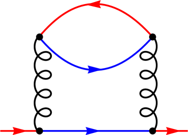
Figure 5: The lowest order diagram for the self-energy that is constructed from the effective Hamiltonian with the matrix elements shown in Fig. 4(b). Here red (blue) color corresponds to $\sigma=+1$ ($\sigma=-1$) Fermi surface. Inversion of the colors yields the self-energy for $\sigma=-1$ electrons. The wiggly lines correspond to the contact interaction defined in Eq. (32). We use this diagram for the self-consistent Born approximation.

Here we consider the effective interaction with non-zero matrix elements that are given only by the diagram in Fig. 4(b) and its conjugate. The lowest order diagram to the self-energy coming from such an effective interaction is shown in Fig. 5. If we apply the perturbation theory and calculate the corresponding non-analytic correction to $\Omega$, we will restore Eq. (61). In this section we want to go beyond perturbation theory. As a first step towards this goal, we treat the diagram in Fig. 5 self-consistently, i.e. we dress all electron Green functions by corresponding self-energies:

$$G_{\sigma}(i\omega,\bm{p})\equiv G_{\sigma}(i\omega,\delta p,\bm{n})$$

$$\hskip 44.0pt=\frac{|\sigma,\bm{n}\rangle\langle\sigma,\bm{n}|}{i\omega-v_{F}\,\delta p-\Sigma_{\sigma}(i\omega,\delta p,\bm{n})},$$ (73)

where $\bm{p}=\bm{k}_{\sigma}+\bm{n}\,\delta p$, see Fig. 1(a), $\bm{k}_{\sigma}$ is the projection of $\bm{p}$ onto the Fermi surface $\mathcal{FS}_{\sigma}$, $\bm{n}$ is the outward normal to $\mathcal{FS}_{\sigma}$ at $\bm{k}_{\sigma}$, $\delta p$ is extended to the interval $(-\infty,\infty)$, $\omega$ is the fermionic Matsubara frequency, and $|\sigma,\bm{n}\rangle$ is given by Eq. (5), $v_{F}$ is the Fermi velocity at zero spin splitting. In Eq. (73) we use that the interband backscattering does not alter the single-particle spinors because the backscattering matrix elements equal unity in absolute value, $|M_{+-}(\pm\bm{n})|=1$, see Eq. (60). So far, we only dress the electron Green functions leaving the effective interaction as contact interaction, see Eq. (32), and also neglecting the interaction vertex corrections. This kind of approximations are usually referred to as self-consistent Born approximations (SCBA). The SCBA self-energy shown in Fig. 5 then reads:

$$\Sigma_{\sigma}(z)=u^{2}P_{-\sigma\sigma}(z)G_{-\sigma}(z),$$ (74)

where $P_{\sigma\sigma^{\prime}}(z)$ is the particle-hole bubble:

$$P_{\sigma\sigma^{\prime}}(z)=-{\rm Tr}\left\{G_{\sigma}(z)G_{\sigma^{\prime}}(-z)\right\}.$$ (75)

Note that the Green functions in Eqs. (74) and (75) are dressed by corresponding self-energies, see Eq. (73).

Here we require the asymptotics of the dressed Green function $G_{\sigma}(\tau,\bm{r})$ at $\tau\gg 1/E_{F}$ and $r\gg\lambda_{F}$:

$$G_{\sigma}(\tau,\bm{r})\approx\left(\frac{1}{\lambda_{F}r}\right)^{\frac{D-1}{2}}\left[e^{i\left(k_{\sigma}(\bm{n}_{\bm{r}})r-\vartheta\right)}\mathcal{G}_{\sigma}(\tau,r,\bm{n}_{\bm{r}})\right.$$

$$\hskip 10.0pt\left.+e^{-i\left(k_{\sigma}(-\bm{n}_{\bm{r}})r-\vartheta\right)}\mathcal{G}_{\sigma}(\tau,-r,-\bm{n}_{\bm{r}})\right],\,\,\,\bm{n}_{\bm{r}}=\frac{\bm{r}}{r},$$ (76)

$$\mathcal{G}_{\sigma}(\tau,x,\bm{n})=T\sum\limits_{\omega}\int\limits_{-\infty}^{\infty}\frac{d\delta p}{2\pi}e^{i\delta px-i\omega\tau}G_{\sigma}(i\omega,\delta p,\bm{n}),$$ (77)

where $\vartheta$ is given by Eq. (19), $\lambda_{F}$ is the Fermi wavelength, and $\mathcal{G}_{\sigma}(\tau,x,\bm{n})$ is the one-dimensional Fourier transform of $G_{\sigma}(i\omega,\delta p,\bm{n})$, see Eq. (73). The summation over Matsubara frequencies $\omega$ in Eq. (77) corresponds to finite temperatures $T>0$. If we neglect the self-energy in Eq. (73), then Eq. (76) transforms into Eq. (18) that we derived for the free electron Green function. As the derivation of Eq. (76) is similar to the derivation of Eq. (18) in many aspects, we refer to Appendix for details.

First, we separate the spinors using Eqs. (73) and (77):

$$\mathcal{G}_{\sigma}(\tau,x,\bm{n})=|\sigma,\bm{n}\rangle\langle\sigma,\bm{n}|g_{\sigma}(\tau,x,\bm{n}),$$ (78)

where $g_{\sigma}(\tau,x,\bm{n})$ is a scalar 1D Green function:

$$g_{\sigma}(\tau,x,\bm{n})$$

$$\hskip 10.0pt=T\sum\limits_{\omega}\int\limits_{-\infty}^{\infty}\frac{d\delta p}{2\pi}\frac{e^{i\delta px-i\omega\tau}}{i\omega-v_{F}\delta p-\Sigma_{\sigma}(i\omega,\delta p,\bm{n})}.$$ (79)

Using Eq. (76) in Eq. (75), we find the asymptotics of the particle-hole bubble $P_{-\sigma\sigma}(z)$:

$$P_{-\sigma\sigma}(\tau,\bm{r})\approx-\left(\frac{1}{\lambda_{F}r}\right)^{D-1}\left[e^{-2i\vartheta}e^{ir(k_{-\sigma}(\bm{n}_{\bm{r}})+k_{\sigma}(-\bm{n}_{\bm{r}}))}g_{-\sigma}(\tau,r,\bm{n}_{\bm{r}})g_{\sigma}(-\tau,r,-\bm{n}_{\bm{r}})\right.$$

$$\hskip 110.0pt\left.+e^{2i\vartheta}e^{-ir(k_{-\sigma}(-\bm{n}_{\bm{r}})+k_{\sigma}(\bm{n}_{\bm{r}}))}g_{-\sigma}(\tau,-r,-\bm{n}_{\bm{r}})g_{\sigma}(-\tau,-r,\bm{n}_{\bm{r}})\right].$$ (80)

Here we used the matrix elements at $\bm{B}=0$, see Eq. (60), because we calculate the leading non-analytic contribution. Then we substitute Eq. (80) into Eq. (74) and use Eq. (76) for the Green function to represent the self-energy in the following form:

$$\Sigma_{\sigma}(\tau,\bm{r})\approx\left(\frac{1}{\lambda_{F}r}\right)^{\frac{D-1}{2}}$$

$$\times\left[e^{i(k_{\sigma}(\bm{n}_{\bm{r}})r-\vartheta)}\mathcal{S}_{\sigma}(\tau,r,\bm{n}_{\bm{r}})\,|\sigma,\bm{n}_{\bm{r}}\rangle\langle\sigma,\bm{n}_{\bm{r}}|\right.$$

$$+\left.e^{-i(k_{\sigma}(-\bm{n}_{\bm{r}})r-\vartheta)}\mathcal{S}_{\sigma}(\tau,-r,-\bm{n}_{\bm{r}})\,|\sigma,-\bm{n}_{\bm{r}}\rangle\langle\sigma,-\bm{n}_{\bm{r}}|\right],$$ (81)

where $\mathcal{S}_{\sigma}(\tau,x,\bm{n})$ is the following function:

$$\mathcal{S}_{\sigma}(\tau,x,\bm{n})=-\frac{u^{2}e^{-i\sigma\Delta(\bm{n})x}}{\left|\lambda_{F}x\right|^{D-1}}$$

$$\hskip 20.0pt\times g_{-\sigma}(\tau,x,\bm{n})g_{-\sigma}(\tau,-x,-\bm{n})g_{\sigma}(-\tau,x,-\bm{n}),$$ (82)

$$\Delta(\bm{n})=k_{+}(\bm{n})-k_{+}(-\bm{n})+k_{-}(-\bm{n})-k_{-}(\bm{n})$$

$$\hskip 20.0pt\approx\frac{2}{v_{F}}\left(\beta(\bm{n})-\beta(-\bm{n})\right)\approx\frac{4}{v_{F}}\frac{\mbox{\boldmath{$\beta$}}_{SO}(\bm{n})\cdot\bm{B}}{\beta_{SO}(\bm{n})}.$$ (83)

Here, we used Eqs. (9) and (59) to simplify $\Delta(\bm{n})$. Notice that Eq. (81) has exactly the same form as Eq. (76) for the Green function. This means that $\mathcal{S}_{\sigma}(\tau,x,\bm{n})$ is just a 1D Fourier transform of the self-energy:

$$\mathcal{S}_{\sigma}(\tau,x,\bm{n})=T\sum\limits_{\omega}\int\limits_{-\infty}^{\infty}\frac{d\delta p}{2\pi}e^{i\delta p\,x-i\omega\tau}\Sigma_{\sigma}(i\omega,\delta p,\bm{n}).$$ (84)

Equation (82) provides the self-energy as a function of $g_{\sigma}(\tau,x,\bm{n})$ which is itself connected to the self-energy via Eq. (79).

V.2 Limit of strong interaction

We expect a FQPT at large value of the dimensionless interaction parameter $g\gg 1$. In this regime, the self-energy dominates over the single-particle terms in the Green function, so we can simplify Eq. (79):

$$g_{\sigma}(\tau,x,\bm{n})\approx T\sum\limits_{\omega}\int\limits_{-\infty}^{\infty}\frac{d\delta p}{2\pi}\frac{e^{i\delta px-i\omega\tau}}{-\Sigma_{\sigma}(i\omega,\delta p,\bm{n})}.$$ (85)

Taking the convolution of $\mathcal{S}_{\sigma}(\tau,x,\bm{n})$ and $g_{\sigma}(\tau,x,\bm{n})$ given by Eqs. (84) and (85), respectively, we find:

$$-\delta(\tau)\delta(x)$$

$$\hskip 10.0pt=\int d\tau^{\prime}dx^{\prime}\,g_{\sigma}(\tau-\tau^{\prime},x-x^{\prime},\bm{n})\mathcal{S}_{\sigma}(\tau^{\prime},x^{\prime},\bm{n}).$$ (86)

Substituting Eq. (82) for the self-energy in Eq. (86), we find the self-consistent equation for the reduced Green function $g_{\sigma}(\tau,x,\bm{n})$ in the limit of strong electron-electron interaction:

$$\delta(\tau)\delta(x)=u^{2}\int d\tau^{\prime}dx^{\prime}\,g_{\sigma}(\tau-\tau^{\prime},x-x^{\prime},\bm{n})g_{\sigma}(-\tau^{\prime},x^{\prime},-\bm{n})g_{-\sigma}(\tau^{\prime},x^{\prime},\bm{n})g_{-\sigma}(\tau^{\prime},-x^{\prime},-\bm{n})\frac{e^{-i\sigma\Delta(\bm{n})x^{\prime}}}{|\lambda_{F}x^{\prime}|^{D-1}}.$$ (87)

V.3 Solutions at $B=0$

First, we analyze the solutions of Eq. (87) at zero magnetic field $\bm{B}=0$ when $\Delta(\bm{n})=0$, see Eq. (83). First of all, we can drop the dependence of the reduced Green function on $\bm{n}$, because there is no explicit dependence on $\bm{n}$ in Eq. (87) if $\Delta(\bm{n})=0$:

$$g_{\sigma}(\tau,x,\bm{n})=g_{\sigma}(\tau,x).$$ (88)

Second, we observe that Eq. (87) is free from any energy or momentum scales which results in the scale invariance (conformal symmetry) of Eq. (87) with respect to independent reparametrization of time and coordinate:

$$\tau\to\ell_{1}\tau,\,\,x\to\ell_{2}x,$$ (89)

where $\ell_{1}$ and $\ell_{2}$ are arbitrary real numbers. Applying this reparametrization to Eq. (87), one can show that the Green function with rescaled coordinates $g_{\sigma}(\ell_{1}\tau,\ell_{2}x)$ is just proportional to $g_{\sigma}(\tau,x)$:

$$g_{\sigma}(\ell_{1}\tau,\ell_{2}x)=\frac{g_{\sigma}(\tau,x)}{|\ell_{1}|^{2d_{1}}|\ell_{2}|^{2d_{2}}},\,\,d_{1}=\frac{1}{4},\,\,d_{2}=\frac{3-D}{8},$$ (90)

where $d_{1}$ and $d_{2}$ are the temporal and spatial scaling dimensions. Equation (90) implies the power-law scaling of the Green function $g_{\sigma}(\tau,x)$ with respect to time and coordinate:

$$g_{\sigma}(\tau,x)\propto\frac{1}{|\tau|^{2d_{1}}}\frac{1}{|x|^{2d_{2}}}.$$ (91)

Thus, we see that we can separate the variables and represent Eq. (87) at $\Delta(\bm{n})=0$ as the product of two independent Dyson equations:

$$g_{\sigma}(\tau,x)=\mathfrak{g}(\tau)\gamma_{\sigma}(x),$$ (92)

$$\delta(\tau)=\int\limits_{-\infty}^{\infty}d\tau^{\prime}\,\mathfrak{g}(\tau-\tau^{\prime})\mathfrak{g}(-\tau^{\prime})\mathfrak{g}^{2}(\tau^{\prime}),$$ (93)

$$\delta(x)=u^{2}\int\limits_{-\infty}^{\infty}dx^{\prime}\,\gamma_{\sigma}(x-x^{\prime})\frac{\gamma_{\sigma}(-x^{\prime})\gamma^{2}_{-\sigma}(x^{\prime})}{|\lambda_{F}x^{\prime}|^{D-1}}.$$ (94)

Equation (93) is the well-known Dyson equation of the Sachdev-Ye-Kitaev (SYK) model [65, 66, 67] which can be applied to describe the strange metal phase in cuprates [67, 68]. In Ref. [58] we found that this model can emerge in strongly interacting electron systems with multiple Fermi surfaces. The zero temperature solution of this equation is the following:

$$\mathfrak{g}(\tau)=\frac{1}{(4\pi)^{\frac{1}{4}}}\frac{{\rm sgn}(\tau)}{|\tau|^{\frac{1}{2}}}.$$ (95)

In fact, this solution can be easily generalized to the case of finite temperature $T$:

$$\mathfrak{g}(\tau)=\frac{{\rm sgn}(\tau)}{(4\pi)^{\frac{1}{4}}}\left|\frac{\pi T}{\sin(\pi T\tau)}\right|^{\frac{1}{2}},$$ (96)

where $\tau\in(-1/T,1/T)$. The factor ${\rm sgn}(\tau)$ is needed here to satisfy the antiperiodicity of the electron Green function:

$$G_{\sigma}\left(\tau+\frac{1}{T},\bm{r}\right)=-G_{\sigma}(\tau,\bm{r}).$$ (97)

Equation (94) is similar to the SYK equation (93) and can be solved in terms of the power-law functions:

$$\gamma_{\sigma}(x)=C_{D}\frac{i\,{\rm sgn}(x)}{|x|^{2d_{2}}},\,\,d_{2}=\frac{3-D}{8},$$ (98)

$$C_{D}=\left[\frac{D+1}{8\pi u^{2}}\lambda_{F}^{D-1}\tan\left(\frac{\pi}{2}\frac{3-D}{4}\right)\right]^{\frac{1}{4}}.$$ (99)

Here we assume that the proportionality coefficient $C_{D}$ is the same for both spin-split bands, so $\gamma_{\sigma}(x)$ is independent of $\sigma$ in this case. This assumption is reasonable because the spin splitting is much smaller than the Fermi energy.

Substituting Eqs. (96) and (98) into Eq. (76), we find the asymptotic form of the SCBA Green function:

$$G_{\sigma}(\tau,\bm{r})\approx\frac{C_{D}}{\lambda_{F}^{\frac{D-1}{2}}}\frac{\mathfrak{g}(\tau)}{r^{\frac{D+1}{4}}}\left[e^{i\left(k_{\sigma}(\bm{n}_{\bm{r}})r-\vartheta+\frac{\pi}{2}\right)}|\sigma,\bm{n}_{\bm{r}}\rangle\langle\sigma,\bm{n}_{\bm{r}}|\right.$$

$$\hskip 20.0pt+\left.e^{-i\left(k_{\sigma}(-\bm{n}_{\bm{r}})r-\vartheta+\frac{\pi}{2}\right)}|\sigma,-\bm{n}_{\bm{r}}\rangle\langle\sigma,-\bm{n}_{\bm{r}}|\right],$$ (100)

where the $\pi/2$ phase is due to the $i\,{\rm sgn}(x)$ phase term in Eq. (98). Equation (100) has a certain phase freedom upon a small translation $r\to r+a$, $a\sim\lambda_{F}$. Such a translation does not change the asymptotics of the power-law tail because $r\gg\lambda_{F}$ but it results in the phase shift in the oscillatory factors. In other words, the phase cannot be determined self-consistently from the long-range infrared limit. Here we derive it from the particle-hole symmetry which is exact close to the Fermi surface, so we conclude that the phase has to be just $-\vartheta$. The true asymptotics of the particle-hole symmetric Matsubara Green function with positively defined spectral function then reads:

$$G_{\sigma}(\tau,\bm{r})\approx\frac{C_{D}}{\lambda_{F}^{\frac{D-1}{2}}}\frac{\mathfrak{g}(\tau)}{r^{\frac{D+1}{4}}}\left[e^{i\left(k_{\sigma}(\bm{n}_{\bm{r}})r-\vartheta\right)}|\sigma,\bm{n}_{\bm{r}}\rangle\langle\sigma,\bm{n}_{\bm{r}}|\right.$$

$$\hskip 20.0pt+\left.e^{-i\left(k_{\sigma}(-\bm{n}_{\bm{r}})r-\vartheta\right)}|\sigma,-\bm{n}_{\bm{r}}\rangle\langle\sigma,-\bm{n}_{\bm{r}}|\right].$$ (101)

The numerical coefficient $C_{D}>0$ is given by Eq. (99).

Here we would like to comment on the case $D=3$ because $C_{D}$ vanishes in this case. In order to resolve this issue, we use the dimensional regularization:

$$C_{D}\approx\sqrt{\frac{\lambda_{F}}{4u}}\delta^{\frac{1}{4}},\,\,D=3-\delta,\,\,\delta\to+0.$$ (102)

Substituting it into Eq. (98) and forgetting about the phase factor (see the paragraph above), we find:

$$\gamma_{\sigma}(x)=\sqrt{\frac{\lambda_{F}}{4u}}\left(\frac{|x|^{\delta}}{\delta}\right)^{-\frac{1}{4}}\approx\sqrt{\frac{\lambda_{F}}{4u}}\left(\frac{1}{\delta}+\ln|x|\right)^{-\frac{1}{4}}.$$ (103)

Here $1/\delta$ comes from the ultraviolet scale $x\sim\lambda_{F}$, so we can write $1/\delta=\ln p_{0}$, where $p_{0}\sim k_{F}$ compensates the dimensionality of $x$:

$$\gamma_{\sigma}(x)=\sqrt{\frac{\lambda_{F}}{4u}}\frac{1}{\left(\ln|p_{0}x|\right)^{\frac{1}{4}}},\,\,p_{0}\sim k_{F}.$$ (104)

As a summary, we provide the Matsubara Green function of strongly interacting 2D and 3D electron gases with arbitrary SO splitting:

$$G_{\sigma}(\tau,\bm{r})\approx\left(\frac{3(\sqrt{2}-1)m^{2}k_{F}}{\pi g^{2}}\right)^{\frac{1}{4}}\frac{e^{i\left(k_{\sigma}(\bm{n}_{\bm{r}})r-\frac{\pi}{4}\right)}|\sigma,\bm{n}_{\bm{r}}\rangle\langle\sigma,\bm{n}_{\bm{r}}|+e^{-i\left(k_{\sigma}(-\bm{n}_{\bm{r}})r-\frac{\pi}{4}\right)}|\sigma,-\bm{n}_{\bm{r}}\rangle\langle\sigma,-\bm{n}_{\bm{r}}|}{4\pi r^{\frac{3}{4}}}$$

$$\hskip 280.0pt\times\left|\frac{\pi T}{\sin(\pi T\tau)}\right|^{\frac{1}{2}}{\rm sgn}(\tau),\,\,D=2,$$ (105)

$$G_{\sigma}(\tau,\bm{r})\approx\frac{k_{F}}{4\pi^{2}}\left(\frac{4\pi m^{2}}{g^{2}}\right)^{\frac{1}{4}}\frac{e^{i\left(k_{\sigma}(\bm{n}_{\bm{r}})r-\frac{\pi}{2}\right)}|\sigma,\bm{n}_{\bm{r}}\rangle\langle\sigma,\bm{n}_{\bm{r}}|+e^{-i\left(k_{\sigma}(-\bm{n}_{\bm{r}})r-\frac{\pi}{2}\right)}|\sigma,-\bm{n}_{\bm{r}}\rangle\langle\sigma,-\bm{n}_{\bm{r}}|}{r\left|\ln(p_{0}r)\right|^{\frac{1}{4}}}$$

$$\hskip 280.0pt\times\left|\frac{\pi T}{\sin(\pi T\tau)}\right|^{\frac{1}{2}}{\rm sgn}(\tau),\,\,D=3,$$ (106)

where $g$ is the dimensionless interaction coupling constant, see Eq. (41). We also provide the Fourier transforms:

$$G_{\sigma}(i\omega,\delta p,\bm{n})=\left(\frac{3\pi}{2}\right)^{\frac{1}{4}}\frac{(\sqrt{2}-1)^{\frac{3}{4}}\Gamma\left(\frac{3}{4}\right)}{2\pi\sqrt{2gE_{F}T}}$$

$$\hskip 60.0pt\times\left|\frac{k_{F}}{\delta p}\right|^{\frac{3}{4}}\frac{\Gamma\left(\frac{\omega}{2\pi T}+\frac{1}{4}\right)}{\Gamma\left(\frac{\omega}{2\pi T}+\frac{3}{4}\right)},\,\,D=2,$$ (107)

$$G_{\sigma}(i\omega,\delta p,\bm{n})=\frac{\pi^{\frac{1}{4}}}{16\sqrt{gE_{F}T}}$$

$$\hskip 10.0pt\times\frac{k_{F}}{|\delta p|}\left(\ln\left|\frac{p_{0}}{\delta p}\right|\right)^{-\frac{5}{4}}\frac{\Gamma\left(\frac{\omega}{2\pi T}+\frac{1}{4}\right)}{\Gamma\left(\frac{\omega}{2\pi T}+\frac{3}{4}\right)},\,\,D=3,$$ (108)

where $\omega=\pi T(2n+1)$ is the Matsubara frequency, with $n$ being an integer, and, again, $p_{0}\sim k_{F}$.

These calculations have been performed within the SCBA. However, the emergent conformal symmetry makes this approximation exact, see Ref. [58] for details. In particular, the interaction vertex correction and the dressing of the effective interaction only lead to the renormalization of the interaction parameter $g$, while the scaling dimensions $d_{1}$ and $d_{2}$ remain the same. In this paper we consider $g$ as a phenomenological parameter, so its renormalizations are not important for us. The only condition that is implied here is that $g\gg 1$ close to the FQPT, so we can apply the limit of strong interaction.

V.4 Solutions at finite $\bm{B}$

If $\bm{B}$ is finite, then Eq. (87) contains an oscillatory term making the self-energy irrelevant at large distance $x\gg 1/\Delta(\bm{n})$, so we expect Fermi liquid behavior at such distances. At small distances $x\ll 1/\Delta(\bm{n})$ the oscillatory term is not important and the solutions, given by Eqs. (105)–(106), are still valid. Following this reasoning, the Fourier transforms Eqs. (107)–(108) are valid if $\delta p\gg\Delta(\bm{n})$, where $\bm{n}$ here labels the direction of $\bm{p}$.

Another important limitation of Eqs. (105)–(108) comes from the assumption that the self-energy $\Sigma_{\sigma}(i\omega,\delta p,\bm{n})$ dominates over the single-particle terms $i\omega-v_{F}\delta p$ which we neglected in Eq. (85). All in all, the non-Fermi liquid regime corresponds to the following constrained region:

$$\Delta(\bm{n})\ll\delta p\ll k_{F},\,\,w(\delta p)\ll\omega\ll W(\delta p),$$ (109)

$$w(\delta p)=\frac{E_{F}}{g}\left|\frac{\delta p}{k_{F}}\right|^{\frac{1}{2}},\,W(\delta p)=gE_{F}\left|\frac{\delta p}{k_{F}}\right|^{\frac{3}{2}},\,D=2,$$ (110)

$$w(\delta p)=\frac{E_{F}}{g}\left(\ln\left|\frac{k_{F}}{\delta p}\right|\right)^{-\frac{5}{2}},$$

$$\hskip 12.0ptW(\delta p)=gE_{F}\left(\frac{\delta p}{k_{F}}\right)^{2}\left(\ln\left|\frac{k_{F}}{\delta p}\right|\right)^{\frac{5}{2}},\,D=3,$$ (111)

where we used $p_{0}\approx k_{F}$ for $D=3$. Here, it is required that $W(\delta p)\gg w(\delta p)$ which further constrains $\delta p$:

$$\delta p\gg\delta p^{*},$$ (112)

$$\delta p^{*}=\frac{k_{F}}{g^{2}},\,D=2,$$ (113)

$$\delta p^{*}=\frac{k_{F}}{g\left(\ln g\right)^{\frac{5}{2}}},\,D=3.$$ (114)

As $g\gg 1$ close to the FQPT, the scale $\delta p^{*}$ is very small. Here we see that at the very deep infrared limit $\delta p\lesssim\delta p^{*}$ the Fermi liquid is restored. This also means that at $\Delta(\bm{n})\ll\delta p^{*}$ the non-analyticity can be correctly estimated by the perturbative approach that we considered in the previous section. The most interesting regime corresponds to $\Delta(\bm{n})\gg\delta p^{*}$ where the dominant contribution to the thermodynamic potential comes from the quantum states that are strongly affected by the interaction. In the next section we calculate the thermodynamic potential $\Omega$ in this regime:

$$\Delta(\bm{n})\gg\delta p^{*}.$$ (115)

VI Thermodynamic potential

In the preceding section we calculated the electron Green function of 2DEG and 3DEG with arbitrary SO splitting in the strongly interacting regime $g\gg 1$, see Eqs. (105)–(108), and we also defined the crossover region with the Fermi liquid, see Eqs. (109) and (115). The Fermi liquid contribution to the non-analyticity is calculated in Sec. IV. Here we address the contribution coming from the strongly correlated region of the phase space, see Eqs. (109) and (115).

In order to calculate the thermodynamic potential $\Omega$, we consider the following energy functional $\Omega(\Sigma,G)$:

$$\Omega(\Sigma,G)=-{\rm Tr}\ln\left(G_{0}^{-1}-\Sigma\right)-{\rm Tr}\left(\Sigma G\right)-\Phi(G),$$ (116)

where ${\rm Tr}$ is the trace over all indexes and $\Phi(G)$ the Luttinger-Ward functional. The saddle point of $\Omega(\Sigma,G)$ yields the Dyson equation and the equation for the electron self-energy:

$$0=\frac{\delta\Omega(\Sigma,G)}{\delta\Sigma_{\sigma}}=\left(G_{0}^{-1}-\Sigma_{\sigma}\right)^{-1}-G_{\sigma},$$ (117)

$$0=\frac{\delta\Omega(\Sigma,G)}{\delta G_{\sigma}}=-\Sigma_{\sigma}-\frac{\delta\Phi(G)}{\delta G_{\sigma}}.$$ (118)

Comparing Eq. (74) with Eq. (118), we reconstruct the Luttinger-Ward functional:

$$\Phi(G)=\frac{u^{2}}{2}\int dz\,\left[{\rm Tr}\left\{G_{+}(z)G_{-}(-z)\right\}\right]^{2}.$$ (119)

The thermodynamic potential $\Omega$ is given by the saddle-point value of the functional $\Omega(\Sigma,G)$:

$$\Omega={\rm Tr}\ln G+3\Phi(G),$$ (120)

where $G$ is the Matsubara Green function. Here we used that $\Sigma$ satisfies Eq. (74), so that $-{\rm Tr}(\Sigma G)=4\Phi(G)$.

VI.1 The logarithmic term

Let us first calculate ${\rm Tr}\ln G$:

$$\Omega_{1}\equiv{\rm Tr}\ln G=\sum\limits_{\sigma}T\sum\limits_{\omega}\int\frac{d\bm{p}}{(2\pi)^{D}}\ln\left(G_{\sigma}(i\omega,\delta p)\right).$$ (121)

Here we assume that Eq. (115) is satisfied, so the quantum critical region is given by the constraints Eqs. (109)–(111).

We start from the low temperature regime:

$$T\ll W(\Delta(\bm{n})).$$ (122)

In this case there are many Matsubara frequencies in the window $\omega\in(w(\Delta(\bm{n})),W(\Delta(\bm{n}))$, so we can approximate the sum over frequencies by an integral. For the same reason, we can also expand the gamma functions in Eqs. (107)–(108) with respect to the large ratio $\omega/(2\pi T)$ such that $\ln G_{\sigma}(i\omega,\delta p)$ takes the following form:

$$\ln G_{\sigma}(i\omega,\delta p)=\frac{3}{4}\ln\left|\frac{k_{F}}{\delta p}\right|-\frac{1}{2}\ln|\omega|+{\rm const},\,D=2,$$ (123)

$$\ln G_{\sigma}(i\omega,\delta p)=\ln\left|\frac{k_{F}}{\delta p}\right|-\frac{5}{4}\ln\ln\left|\frac{p_{0}}{\delta p}\right|$$

$$\hskip 90.0pt-\frac{1}{2}\ln|\omega|+{\rm const},\,D=3.$$ (124)

The sum over $\sigma$ in Eq. (121) yields just a factor of $2$. As $\ln G_{\sigma}(i\omega,\delta p)$ is an even function of $\omega$ and $\delta p$, we can integrate over the positive intervals, i.e. $\delta p\in(\Delta(\bm{n}),k_{F})$ and $\omega\in(0,W(\delta p))$. Note that we extend the integration over $\omega$ all the way to zero frequency because $W(\delta p)\gg T$ and $W(\delta p)\gg w(\delta p)$. This allows us to represent Eq. (121) in the following form:

$$\Omega_{1}(\bm{B})=2\int\limits_{0}^{2\pi}\frac{d\phi}{2\pi}2\int\limits_{\Delta(\phi)}^{k_{F}}\frac{k_{F}\,d\delta p}{2\pi}2\int\limits_{0}^{W(\delta p)}\frac{d\omega}{2\pi}$$

$$\hskip 60.0pt\times\left(\frac{3}{4}\ln\left|\frac{k_{F}}{\delta p}\right|-\frac{1}{2}\ln|\omega|\right),\,D=2,$$ (125)

$$\Omega_{1}(\bm{B})=2\int\frac{d\bm{n}}{4\pi}2\int\limits_{\Delta(\bm{n})}^{k_{F}}\frac{k_{F}^{2}\,d\delta p}{2\pi^{2}}2\int\limits_{0}^{W(\delta p)}\frac{d\omega}{2\pi}$$

$$\hskip 10.0pt\times\left(\ln\left|\frac{k_{F}}{\delta p}\right|-\frac{5}{4}\ln\ln\left|\frac{p_{0}}{\delta p}\right|-\frac{1}{2}\ln|\omega|\right),\,D=3.$$ (126)

Next, we take the integral over $\omega$ with logarithmic accuracy. In particular, we neglect the $\ln\ln|\delta p|$ term in the 3D case compared to the $\ln|\delta p|$ term:

$$\Omega_{1}(\bm{B})=\frac{2k_{F}^{2}}{\pi^{2}}\int\limits_{0}^{2\pi}\frac{d\phi}{2\pi}\int\limits_{\Delta(\phi)}^{k_{F}}\frac{d\delta p}{k_{F}}W(\delta p)$$

$$\hskip 40.0pt\times\left(\frac{3}{4}\ln\left|\frac{k_{F}}{\delta p}\right|-\frac{1}{2}\ln|W(\delta p)|\right),\,D=2,$$ (127)

$$\Omega_{1}(\bm{B})=\frac{2k_{F}^{3}}{\pi^{3}}\int\frac{d\bm{n}}{4\pi}\int\limits_{\Delta(\bm{n})}^{k_{F}}\frac{d\delta p}{k_{F}}W(\delta p)$$

$$\hskip 40.0pt\times\left(\ln\left|\frac{k_{F}}{\delta p}\right|-\frac{1}{2}\ln|W(\delta p)|\right),\,D=3.$$ (128)

Then substituting $W(\delta p)$, see Eqs. (110)–(111), we find:

$$\Omega_{1}(\bm{B})=\frac{3k_{F}^{2}gE_{F}}{\pi^{2}}\int\limits_{0}^{2\pi}\frac{d\phi}{2\pi}$$

$$\hskip 50.0pt\times\int\limits_{\Delta(\phi)}^{k_{F}}\frac{d\delta p}{k_{F}}\left|\frac{\delta p}{k_{F}}\right|^{\frac{3}{2}}\ln\left|\frac{k_{F}}{\delta p}\right|,\,D=2,$$ (129)

$$\Omega_{1}(\bm{B})=\frac{4k_{F}^{3}gE_{F}}{\pi^{3}}\int\frac{d\bm{n}}{4\pi}$$

$$\hskip 50.0pt\times\int\limits_{\Delta(\bm{n})}^{k_{F}}\frac{d\delta p}{k_{F}}\left|\frac{\delta p}{k_{F}}\right|^{2}\ln\left|\frac{k_{F}}{\delta p}\right|^{\frac{7}{2}},\,D=3.$$ (130)

Calculating the integrals over $\delta p$ with the logarithmic accuracy and subtracting the part which is independent of $\Delta(\bm{n})$, we find the non-analytic contribution to the thermodynamic potential:

$$\Omega_{1}(\bm{B})=-\frac{6k_{F}^{2}gE_{F}}{5\pi^{2}}$$

$$\hskip 40.0pt\times\int\limits_{0}^{2\pi}\frac{d\phi}{2\pi}\left|\frac{\Delta(\phi)}{k_{F}}\right|^{\frac{5}{2}}\ln\left|\frac{k_{F}}{\Delta(\phi)}\right|,\,D=2,$$ (131)

$$\Omega_{1}(\bm{B})=-\frac{4k_{F}^{3}gE_{F}}{3\pi^{3}}$$

$$\hskip 20.0pt\times\int\frac{d\bm{n}}{4\pi}\left|\frac{\Delta(\bm{n})}{k_{F}}\right|^{3}\left(\ln\left|\frac{k_{F}}{\Delta(\bm{n})}\right|\right)^{\frac{7}{2}},\,D=3.$$ (132)

Finally, we have to calculate the Luttinger-Ward contribution to $\Omega$.

VI.2 Luttinger-Ward contribution

Here we calculate the second part of the thermodynamic potential, see Eq. (120):

$$\Omega_{2}(\bm{B})=3\Phi(G)=\frac{3u^{2}}{2}\!\!\int dz\left[{\rm Tr}\left\{G_{+}(z)G_{-}(-z)\right\}\right]^{2}.$$ (133)

In this case it is more convenient to use the real space representation of the Green function, see Eqs. (105)–(106). Here we will show that $\Omega_{2}(\bm{B})$ yields a subleading correction compared to $\Omega_{1}(\bm{B})$.

Using Eqs. (105)–(106), we find:

$$\left[{\rm Tr}\left\{G_{+}(z)G_{-}(-z)\right\}\right]^{2}\approx\frac{3(\sqrt{2}-1)m^{2}k_{F}}{2^{7}\pi^{5}g^{2}}$$

$$\hskip 30.0pt\times\frac{e^{ir\Delta(\bm{n}_{\bm{r}})}}{r^{3}}\left|\frac{\pi T}{\sin(\pi T\tau)}\right|^{2},\,D=2,$$ (134)

$$\left[{\rm Tr}\left\{G_{+}(z)G_{-}(-z)\right\}\right]^{2}\approx\frac{m^{2}k_{F}^{4}}{2^{5}\pi^{7}g^{2}}$$

$$\hskip 30.0pt\times\frac{e^{ir\Delta(\bm{n}_{\bm{r}})}}{r^{4}\ln(p_{0}r)}\left|\frac{\pi T}{\sin(\pi T\tau)}\right|^{2},\,D=3,$$ (135)

First, we have to translate the conditions given by Eqs. (109)–(111) to constraints on $\tau$ and $r$. We do it via the correspondence $\omega\sim 1/\tau$, $\delta p\sim 1/r$. Thus, in our case the integration region is defined by the following constraints:

$$\tau\gg\overline{\tau}(r)=\frac{1}{W(r^{-1})},\,\,r\ll\frac{1}{\Delta(\bm{n})}.$$ (136)

Here we show only the most important conditions. As in the previous case, we consider small temperatures $T\ll W(\Delta(\bm{n}))$, so we can actually use the $T=0$ approximation. First, we integrate over $\tau$:

$$\int\limits_{\overline{\tau}(r)}^{\frac{1}{T}-\overline{\tau}(r)}d\tau\,\left|\frac{\pi T}{\sin(\pi T\tau)}\right|^{2}\approx 2\int\limits_{\overline{\tau}(r)}^{\infty}\frac{d\tau}{\tau^{2}}=\frac{2}{\overline{\tau}(r)}.$$ (137)

Substituting this in $\Omega_{2}(\bm{B})$, we find:

$$\Omega_{2}(\bm{B})=\frac{9(\sqrt{2}-1)}{16\pi^{2}}gE_{F}k_{F}^{2}\int\limits_{0}^{2\pi}\frac{d\phi}{2\pi}$$

$$\hskip 70.0pt\times\int\limits_{0}^{\infty}\frac{k_{F}dr}{(k_{F}r)^{\frac{7}{2}}}e^{ir\Delta(\phi)},\,D=2,$$ (138)

$$\Omega_{2}(\bm{B})=\frac{3}{2\pi^{2}}gE_{F}k_{F}^{3}\int\frac{d\bm{n}}{4\pi}$$

$$\hskip 30.0pt\times\int\limits_{0}^{\infty}\frac{k_{F}dr}{(k_{F}r)^{4}}\left(\ln(k_{F}r)\right)^{\frac{3}{2}}e^{ir\Delta(\bm{n})},\,D=3.$$ (139)

We substituted $p_{0}\approx k_{F}$ for $D=3$ case. Note that here we do not even have to use the condition $r\ll 1/\Delta(\bm{n})$ because it is effectively satisfied due to the oscillatory term $e^{ir\Delta(\bm{n})}$. The integral over $k_{F}r$ in Eq. (138) is calculated via Eq. (28). As $\Delta(\phi+\pi)=-\Delta(\phi)$, see Eq. (83), then only the real part does not vanish after the integration over $\phi$. The integral in Eq. (139) can be calculated similarly. Here we calculate it with logarithmic accuracy:

$$\int\limits_{0}^{\infty}\frac{k_{F}dr}{(k_{F}r)^{4+\delta}}\left(\ln(k_{F}r)\right)^{\frac{3}{2}}e^{ir\Delta(\bm{n})}$$

$$\approx\left(\ln\left|\frac{k_{F}}{\Delta(\bm{n})}\right|\right)^{\frac{3}{2}}\left|\frac{\Delta(\bm{n})}{k_{F}}\right|^{3+\delta}\frac{i\,{\rm sgn}(\Delta(\bm{n}))+\frac{\pi}{2}\delta}{6\delta},$$ (140)

where we introduced some small $\delta\to 0$. As $\Delta(-\bm{n})=-\Delta(\bm{n})$, the divergent $1/\delta$ part cancels out after the integration over $\bm{n}$, so the physical contribution is finite. In conclusion, we find $\Omega_{2}(\bm{B})$:

$$\Omega_{2}(\bm{B})=\frac{3(\sqrt{2}-1)}{5(2\pi)^{\frac{3}{2}}}gE_{F}k_{F}^{2}$$

$$\hskip 70.0pt\times\int\limits_{0}^{2\pi}\frac{d\phi}{2\pi}\left|\frac{\Delta(\phi)}{k_{F}}\right|^{\frac{5}{2}},\,D=2,$$ (141)

$$\Omega_{2}(\bm{B})=\frac{gE_{F}k_{F}^{3}}{8\pi}$$

$$\hskip 20.0pt\times\int\frac{d\bm{n}}{4\pi}\left|\frac{\Delta(\bm{n})}{k_{F}}\right|^{3}\left(\ln\left|\frac{k_{F}}{\Delta(\bm{n})}\right|\right)^{\frac{3}{2}},\,D=3.$$ (142)

Indeed, compared to $\Omega_{1}(\bm{B})$, see Eqs. (131) and (132), $\Omega_{2}(\bm{B})$ is only subleading, so we can neglect it.

Summing over, the leading non-analyticity in $\Omega$ in the strongly interacting regime $g\gg 1$ close to FQPT is given by the $\Omega_{1}$ contribution, see Eqs. (131) and (132). Here we represent the answer using the angular form-factors $\overline{F}_{D}(\bm{b})$ that are different from the form-factors $F_{D}(\bm{b})$ that appear in the weak coupling regime, see Eq. (64):

$$\delta\Omega(\bm{B})=\frac{6k_{F}^{2}gE_{F}}{5\pi^{2}}\left|\frac{2B}{E_{F}}\right|^{\frac{5}{2}}\ln\left|\frac{2B}{E_{F}}\right|\overline{F}_{2}(\bm{b}),\,D=2,$$ (143)

$$\delta\Omega(\bm{B})=-\frac{32k_{F}^{3}g|B|^{3}}{3\pi^{3}E_{F}^{2}}\left|\ln\left|\frac{E_{F}}{2B}\right|\right|^{\frac{7}{2}}\overline{F}_{3}(\bm{b}),\,D=3,$$ (144)

$$\overline{F}_{D}(\bm{b})=\int\limits_{S_{D-1}}\frac{d\bm{n}}{S_{D-1}}\left|\frac{\mbox{\boldmath{$\beta$}}_{SO}(\bm{n})\cdot\bm{b}}{\beta_{SO}(\bm{n})}\right|^{\frac{D+3}{2}},$$ (145)

where $\bm{b}=\bm{B}/B$. First, we notice that the non-analytic terms are negative and that they are parametrically larger than the Fermi liquid non-analyticity, see Eqs. (62) and (63). The angular form-factor $\overline{F}_{D}(\bm{b})$ due to the SO splitting is different from the one that we considered in the weak coupling regime, see Eq. (64), but it still results in the same physical effect: if the SO splitting breaks the spin rotational symmetry down to $\mathbb{Z}_{2}$, then the ferromagnetic ground state is Ising and the magnetization axis is defined by the direction where the SO splitting and, thus, $\overline{F}_{D}(\bm{b})$ are maximal.

Equations (143) and (144) are valid at very low temperatures when $T\ll W(\Delta(\bm{n}))$. This condition can be rewritten as follows:

$$B\gg B^{*}(T),$$ (146)

$$B^{*}(T)=E_{F}\left|\frac{T}{gE_{F}}\right|^{\frac{2}{3}},\,\,D=2,$$ (147)

$$B^{*}(T)=\frac{E_{F}}{\left(\ln|gE_{F}/T|\right)^{\frac{5}{4}}}\sqrt{\frac{T}{gE_{F}}},\,\,D=3.$$ (148)

If $B\ll B^{*}(T)$, then the electron self-energy at $\omega\sim B$ and $v_{F}\delta p\sim B$ is irrelevant, so the regime $B\ll B^{*}(T)$ corresponds to the Fermi liquid regime and the non-analyticity in $\Omega$ is described by Eqs. (62)–(63). The regime $B\gg B^{*}(T)$ is quantum critical and the non-analyticities are described by Eqs. (143)–(144). The regime $B\sim B^{*}(T)$ corresponds to the crossover between the Fermi-liquid and the non-Fermi-liquid regimes.

In this section we treated the resonant backscattering processes shown in Fig. 4(b) non-perturbatively and found that the non-analytic terms in $\Omega$ remain negative close to the FQPT and that they are strongly enhanced in magnitude compared to the regime of weak interaction. This means that the FQCP separating paramagnetic and ferromagnetic metals is intrinsically unstable even in the presence of arbitrarily complex SO splitting.

VII Spin susceptibility far away and close to FQPT

The non-analytic corrections destabilizing the FQCP separating ferromagnetic and paramagnetic phases can be measured experimentally via the magnetic field dependence of the spin susceptibility $\chi_{ij}(\bm{B})$ in the paramagnetic phase:

$$\chi_{ij}(\bm{B})=-\frac{\partial^{2}\Omega(\bm{B})}{\partial B_{i}\partial B_{j}}.$$ (149)

Deep inside the paramagnetic phase where $g\ll 1$ or $\lambda_{F}\ll a_{B}$, see Eq. (41), the non-analytic correction is given by Eqs. (62)–(63), so the corresponding non-analytic corrections to the spin susceptibility are the following:

$$\delta\chi_{ij}(\bm{B})=\frac{2g^{2}|B|}{\pi v_{F}^{2}}\kappa^{(2)}_{ij}(\bm{b}),\,\,D=2,$$ (150)

$$\delta\chi_{ij}(\bm{B})=-\frac{4g^{2}B^{2}}{\pi^{2}v_{F}^{3}}\ln\left|\frac{2B}{\Lambda}\right|\kappa^{(3)}_{ij}(\bm{b}),\,\,D=3,$$ (151)

$$\kappa^{(D)}_{ij}(\bm{b})$$

$$=\int\limits_{S_{D-1}}\frac{d\bm{n}}{S_{D-1}}\left|\frac{\mbox{\boldmath{$\beta$}}_{SO}(\bm{n})\cdot\bm{b}}{\beta_{SO}(\bm{n})}\right|^{D-1}\frac{\beta_{SO}^{i}(\bm{n})\beta_{SO}^{j}(\bm{n})}{\beta^{2}_{SO}(\bm{n})},$$ (152)

where $\Lambda\sim E_{F}$, $\beta_{SO}^{i}(\bm{n})$ is the $i^{{\rm th}}$ component of the vector $\mbox{\boldmath{$\beta$}}_{SO}(\bm{n})$. These results are valid for $B\gg T$. In the opposite regime $B\ll T$, the non-analyticity is regularized by the temperature. An important feature here is the non-trivial angular dependence of the spin susceptibility on $\bm{b}$ due to the SO splitting, see the angular tensor $\kappa^{(D)}_{ij}(\bm{b})$. Measuring $\kappa^{(D)}_{ij}(\bm{b})$ can resolve the angular dependence of the SO splitting. However, it is not an easy task to measure the non-analytic corrections to the spin susceptibility in the weak coupling regime because they are proportional to $g^{2}$, where $g\ll 1$.

It is much more promising to measure the non-analyticities in the spin susceptibility when the paramagnetic phase is close to the FQPT, such that $g\gg 1$ and we can use the results of Sec. VI, see Eqs. (143)–(144):

$$\delta\chi_{ij}(\bm{B})$$

$$\approx\frac{36\sqrt{2}}{\pi^{2}}mg\ln\left|\frac{E_{F}}{2B}\right|\sqrt{\frac{|B|}{E_{F}}}\,\overline{\kappa}_{ij}^{(2)}(\bm{b}),\,\,D=2,$$ (153)

$$\delta\chi_{ij}(\bm{B})$$

$$\approx\frac{256mg}{\pi^{3}v_{F}}\left|\ln\left(\frac{E_{F}}{2B}\right)\right|^{\frac{7}{2}}|B|\,\overline{\kappa}_{ij}^{(3)}(\bm{b}),\,\,D=3,$$ (154)

$$\overline{\kappa}^{(D)}_{ij}(\bm{b})$$

$$=\int\limits_{S_{D-1}}\frac{d\bm{n}}{S_{D-1}}\left|\frac{\mbox{\boldmath{$\beta$}}_{SO}(\bm{n})\cdot\bm{b}}{\beta_{SO}(\bm{n})}\right|^{\frac{D-1}{2}}\frac{\beta_{SO}^{i}(\bm{n})\beta_{SO}^{j}(\bm{n})}{\beta^{2}_{SO}(\bm{n})}.$$ (155)

These equations are valid if $B\gg B^{*}(T)$, where $B^{*}(T)$ is given by Eqs. (147) and (148). If $B\ll B^{*}(T)$, then the electron self-energy is irrelevant on the scale $\omega\sim B$ and the non-analyticity is given by Eqs. (150) and (151). Here we see that at $B\gg B^{*}(T)$ the non-analytic corrections to the susceptibility are strongly enhanced. In particular, $\delta\chi_{ij}(\bm{B})\propto\sqrt{|B|}$ in a 2DEG and $\delta\chi_{ij}(\bm{B})\propto|B|$ in a 3DEG, which is much easier to detect experimentally than the much weaker non-analyticities far away from the FQPT, see Eqs. (150) and (151). To measure local spin susceptibility one can use, for example, ultrasensitive nitrogen-vacancy center based detectors [69].

VIII Conclusions

In this paper we revisited FQPT in strongly interacting clean 2DEG and 3DEG with arbitrary SO splitting. First of all, we calculated the non-analytic corrections to the thermodynamic potential $\Omega$ with respect to arbitrary spin splitting in the limit of weak electron-electron interaction. So far, this has been done in the literature only for very limited number of special cases [43, 55, 56, 57]. Here we generalized the calculation for arbitrary spin splitting and arbitrary spatial dimension $D>1$, see Eq. (44). The most important outcome of this calculation is that even arbitrarily complex SO splitting is not able to cut the non-analyticity in $\Omega$ with respect to the magnetic field, see Eq. (61). This is a direct consequence of the backscattering processes shown in Fig. 4. Such processes were not taken into account in Ref. [57] where a complicated enough SO splitting is predicted to cut the non-analyticity.

The weak coupling regime cannot be extended to the phase transition point where the electron-electron interaction is very strong. In order to address this regime, we treat the processes in Fig. 4 non-perturbatively and find that there is a sector in the phase space where the electron Green function exhibits strong non-Fermi-liquid behavior. We find that this non-Fermi-liquid sector dominates the non-analytic response at low temperatures. We also find that the non-analyticity remains negative but it is parametrically enhanced from $\delta\Omega\propto-|B|^{D+1}$ in the weak interaction limit to $\delta\Omega\propto-|B|^{\frac{D+3}{2}}$ in the strong coupling regime. In particular, the non-analyticity in interacting 3DEG is enhanced from the marginal $\propto B^{4}\ln|B|$ term in the weak interaction regime to $\propto-|B|^{3}$ close to the FQPT where the interaction is strong. In addition, SO splitting makes the non-analytic corrections strongly anisotropic. In particular, if the SO splitting breaks the spin symmetry down to $\mathbb{Z}_{2}$, then the ferromagnetic ground state is necessarily Ising-like. In this case, all soft fluctuations of the magnetic order parameter are gapped which validates the mean-field treatment of the magnetization. Nevertheless, there is still a gapless fluctuation channel originating from the resonant backscattering processes shown in Fig. 4(b) which contributes to the negative non-analytic terms in $\Omega$ destabilizing the FQCP. Based on our analysis, we conclude that the FQPT in clean metals is always first order regardless of the SO splitting. The non-analytic terms leading to the instability of the FQCP in clean metals can be measured via the non-analytic dependence of the spin susceptibility on the magnetic field both far away, see Eqs. (150) and (151), or close to the FQPT, see Eqs. (153) and (154). The candidate materials are the pressure-tuned 3D ferromagnets ZrZn₂ [59], UGe₂ [60], and many others [62], or density-tuned 2D quantum wells [61].

Appendix A ASYMPTOTICS OF THE GREEN FUNCTION

We start from the Fourier representation of the Green function:

$$G(\tau,\bm{r})=\int\frac{d\bm{p}}{(2\pi)^{D}}e^{i\bm{p}\cdot\bm{r}}G(\tau,\bm{p}),$$ (156)

where $\tau$ is the imaginary time, $\bm{r}$ a $D$-dimensional position vector, and $\bm{p}$ a $D$-dimensional momentum vector. Here we do not indicate any band index because it is fixed. The asymptotics at large $\tau\gg 1/E_{F}$ and large $r=|\bm{r}|\gg\lambda_{F}$ is dominated by the vicinity of the Fermi surface $\mathcal{FS}$, so we can expand the momentum $\bm{p}$ into the momentum $\bm{k}$ on the Fermi surface $\mathcal{FS}$ and the momentum along the outward normal $\bm{n}(\bm{k})$ at $\bm{k}$, see Fig. 1(a):

$$\bm{p}=\bm{k}+\bm{n}(\bm{k})\delta p,\,\,\,\,\bm{k}\in\mathcal{FS},$$ (157)

where $\delta p$ is the distance from $\bm{p}$ to the Fermi surface $\mathcal{FS}$. Notice that $\delta p>0$ ($\delta p<0$) corresponds to the states above (below) the Fermi surface. At large $r\gg 1/k_{F}$, $k_{F}$ is the typical momentum scale on the Fermi surface, we have $\delta p\sim 1/r\ll k_{F}$, so we can approximate the integral over $\bm{p}$ by the integration over a thin layer around the Fermi surface:

$$G(\tau,\bm{r})\approx\int\limits_{-\infty}^{\infty}\frac{d\delta p}{2\pi}\int\limits_{\bm{k}\in\mathcal{FS}}\frac{d\bm{k}}{(2\pi)^{D-1}}$$

$$\hskip 20.0pt\times e^{i\bm{k}\cdot\bm{r}}e^{i\delta p\,\bm{n}(\bm{k})\cdot\bm{r}}G(\tau,\delta p,\bm{k}),$$ (158)

$$G(\tau,\delta p,\bm{k})\equiv G(\tau,\bm{k}+\bm{n}(\bm{k})\delta p).$$ (159)

Here we extended the integral over $\delta p$ to the interval $(-\infty,\infty)$ because the convergence radius of this integral is very short at $r\to\infty$, namely $\delta p\sim 1/r$. Hence, we approximated the initial Fourier transform Eq. (156) by the integral over the fiber bundle $\mathcal{FS}\times(-\infty,\infty)$.

As $r\to\infty$, we can use the stationary phase method to find the asymptotics. First, we evaluate the integral over the Fermi surface. The stationary condition for the phase of the rapidly oscillating factor $e^{i\bm{k}\cdot\bm{r}}$ in Eq. (158) reads:

$$d\bm{k}\cdot\bm{r}=0,$$ (160)

where $d\bm{k}$ is an arbitrary infinitesimal (but non-zero) element of the tangent space $\mathcal{T}(\bm{k})$ attached to the Fermi surface $\mathcal{FS}$ at the point $\bm{k}$. Hence, $\bm{r}$ has to be orthogonal to the whole linear space $\mathcal{T}(\bm{k})$ which has codimension one. This means that the stationary phase condition is satisfied at the points $\bm{k}^{\prime}\in\mathcal{FS}$ where $\bm{r}$ is collinear with the normals $\bm{n}(\bm{k}^{\prime})$:

$$\bm{n}(\bm{k}^{\prime})=s(\bm{k}^{\prime},\bm{n}_{\bm{r}})\bm{n}_{\bm{r}},\,\,\,\,\bm{n}_{\bm{r}}=\frac{\bm{r}}{r},$$ (161)

where $s(\bm{k}^{\prime},\bm{n}_{\bm{r}})=+1$ ($s(\bm{k}^{\prime},\bm{n}_{\bm{r}})=-1$) if the outward normal $\bm{n}(\bm{k}^{\prime})$ and the radius vector $\bm{r}$ are parallel (anti-parallel). We include all such points $\bm{k}^{\prime}$ into a set $\mathcal{P}(\bm{n}_{\bm{r}})$:

$$\mathcal{P}(\bm{n}_{\bm{r}})=\{\bm{k}^{\prime}\in\mathcal{FS}|\bm{n}(\bm{k}^{\prime})=\pm\bm{n}_{\bm{r}}\}.$$ (162)

It is clear that $\mathcal{P}(-\bm{n}_{\bm{r}})=\mathcal{P}(\bm{n}_{\bm{r}})$ and $s(\bm{k}^{\prime},-\bm{n}_{\bm{r}})=-s(\bm{k}^{\prime},\bm{n}_{\bm{r}})$.

At this point we can take the integral over $\delta p$ in Eq. (158):

$$\int\limits_{-\infty}^{\infty}\frac{d\delta p}{2\pi}e^{i\delta p\,\bm{n}(\bm{k}^{\prime})\cdot\bm{r}}G(\tau,\delta p,\bm{k}^{\prime})=\mathcal{G}(\tau,s(\bm{k}^{\prime},\bm{n}_{\bm{r}})r,\bm{k}^{\prime}),$$ (163)

where we used that $\bm{k}^{\prime}\in\mathcal{P}(\bm{n}_{\bm{r}})$ and $s(\bm{k}^{\prime},\bm{n}_{\bm{r}})=\bm{n}(\bm{k}^{\prime})\cdot\bm{n}_{\bm{r}}=\pm 1$, see Eq. (161). Here $\mathcal{G}(\tau,x,\bm{k})$ is the 1D Fourier transform of the Green function:

$$\mathcal{G}(\tau,x,\bm{k})=\int\limits_{-\infty}^{\infty}\frac{d\delta p}{2\pi}e^{i\delta p\,x}G(\tau,\delta p,\bm{k}),\,\,\bm{k}\in\mathcal{FS}.$$ (164)

Note that such a 1D Fourier transform is generally dependent on the point $\bm{k}\in\mathcal{FS}$. Substituting this into Eq. (158), we find:

$$G(\tau,\bm{r})\approx\sum\limits_{\bm{k}^{\prime}\in\mathcal{P}(\bm{n}_{\bm{r}})}e^{i\bm{k}^{\prime}\cdot\bm{r}}J_{\bm{k}^{\prime}}(r)\mathcal{G}(\tau,s(\bm{k}^{\prime},\bm{n}_{\bm{r}})r,\bm{k}^{\prime}),$$ (165)

$$J_{\bm{k}^{\prime}}(r)=\int\limits_{\bm{k}\in\mathcal{FS}}\frac{d\bm{k}}{(2\pi)^{D-1}}e^{i(\bm{k}-\bm{k}^{\prime})\cdot\bm{r}}.$$ (166)

The function $J_{\bm{k}^{\prime}}(r)$ appears due to the integration over a small vicinity of a point $\bm{k}^{\prime}\in\mathcal{P}(\bm{n}_{\bm{r}})$.

The integral $J_{\bm{k}^{\prime}}(r)$ converges due to the finite curvature of the Fermi surface at $\bm{k}^{\prime}$. This is true even if the interaction is very strong such that the Fermi surface becomes critical. In order to evaluate this integral, it is convenient to introduce an auxiliary function $\varepsilon(\bm{p})$ with the following properties:

$$\varepsilon(\bm{p})=0\,\,{\rm if}\,\,\bm{p}\in\mathcal{FS},$$ (167)

$$\bm{v}(\bm{p})=\frac{\partial\varepsilon(\bm{p})}{\partial\bm{p}}\neq 0\,\,{\rm if}\,\,\bm{p}\in\mathcal{FS}.$$ (168)

We notice here that there are infinitely many choices for such a function but we will show that the result is independent of the choice. In case of a free electron gas the natural choice for $\varepsilon(\bm{p})$ is the electron dispersion. The condition Eq. (168) is required to generate the outward normal $\bm{n}(\bm{k})$ at each point $\bm{k}\in\mathcal{FS}$:

$$\bm{v}(\bm{k})=v(\bm{k})\bm{n}(\bm{k}),\,\,\bm{k}\in\mathcal{FS}.$$ (169)

Here $v(\bm{k})\neq 0$ for all $\bm{k}\in\mathcal{FS}$.

Consider two close points $\bm{k}\in\mathcal{FS}$ and $\bm{k}^{\prime}\in\mathcal{FS}$. According to Eq. (167), we can write:

$$\varepsilon(\bm{k})=\varepsilon(\bm{k}^{\prime})=0.$$ (170)

Using the Taylor series expansion, we find:

$$0=\varepsilon(\bm{k})\approx\varepsilon(\bm{k}^{\prime})+(\bm{k}-\bm{k}^{\prime})\cdot\bm{v}(\bm{k}^{\prime})$$

$$+\frac{1}{2}(\bm{k}-\bm{k}^{\prime})^{T}R(\bm{k}^{\prime})(\bm{k}-\bm{k}^{\prime}),$$ (171)

$$R_{ij}(\bm{p})=\frac{\partial^{2}\varepsilon(\bm{p})}{\partial p_{i}\partial p_{j}},$$ (172)

where we used the matrix notations in Eq. (171), and the superscript ^T stands for transposition. Substituting Eq. (169) into Eq. (171), we find:

$$(\bm{k}-\bm{k}^{\prime})\cdot\bm{n}(\bm{k}^{\prime})\approx-(\bm{k}-\bm{k}^{\prime})^{T}\frac{R(\bm{k}^{\prime})}{2v(\bm{k}^{\prime})}(\bm{k}-\bm{k}^{\prime}).$$ (173)

In Eq. (166) $\bm{k}^{\prime}\in\mathcal{P}(\bm{n}_{\bm{r}})$, so $\bm{n}(\bm{k}^{\prime})$ satisfies Eq. (161). This allows us to write:

$$(\bm{k}-\bm{k}^{\prime})\cdot\bm{r}\approx-s(\bm{k}^{\prime},\bm{n}_{\bm{r}})r(\bm{k}-\bm{k}^{\prime})^{T}\frac{R(\bm{k}^{\prime})}{2v(\bm{k}^{\prime})}(\bm{k}-\bm{k}^{\prime}).$$ (174)

The expression is quadratic with respect to the small difference $\bm{k}-\bm{k}^{\prime}$. At large $r$ the convergence radius of the integral $J_{\bm{k}^{\prime}}(r)$ scales as $|\bm{k}-\bm{k}^{\prime}|\propto 1/\sqrt{r}$, so we indeed have to integrate over a small vicinity of $\bm{k}^{\prime}\in\mathcal{P}(\bm{n}_{\bm{r}})$ and the Taylor expansion is valid. Equation (174) also shows that the component of $\bm{k}-\bm{k}^{\prime}$ along the normal $\bm{n}(\bm{k}^{\prime})$ is only quadratic with respect to $\bm{k}-\bm{k}^{\prime}$, so at a given accuracy we can approximate $\bm{k}-\bm{k}^{\prime}$ on the right-hand side of Eq. (174) by its orthogonal projection onto the tangent space $\mathcal{T}(\bm{k}^{\prime})$:

$$J_{\bm{k}^{\prime}}(r)\approx\int\limits_{\mbox{\boldmath{$\kappa$}}\in\mathcal{T}(\bm{k}^{\prime})}\frac{d\mbox{\boldmath{$\kappa$}}}{(2\pi)^{D-1}}e^{-irs(\bm{k}^{\prime},\bm{n}_{\bm{r}})\mbox{\boldmath{$\kappa$}}^{T}A(\bm{k}^{\prime})\mbox{\boldmath{$\kappa$}}},$$ (175)

$$A(\bm{k}^{\prime})=\frac{R_{\mathcal{T}}(\bm{k}^{\prime})}{2v(\bm{k}^{\prime})},$$ (176)

where $R_{\mathcal{T}}(\bm{k}^{\prime})$ is the restriction of the tensor $R(\bm{k}^{\prime})$ to the tangent space $\mathcal{T}(\bm{k}^{\prime})$. We reduced the initial integral $J_{\bm{k}^{\prime}}(r)$ to a standard Gaussian integral:

$$J_{\bm{k}^{\prime}}(r)\approx\left(\frac{1}{4\pi r}\right)^{\frac{D-1}{2}}\frac{e^{-i\frac{\pi}{4}s(\bm{k}^{\prime},\bm{n}_{\bm{r}})\mathfrak{S}(A(\bm{k}^{\prime}))}}{\sqrt{|\det A(\bm{k}^{\prime})|}},$$ (177)

$$\mathfrak{S}(A(\bm{k}^{\prime}))=\sum\limits_{i=1}^{D-1}{\rm sgn}(a_{i}),$$ (178)

where $a_{i}$ are all $D-1$ eigenvalues of the symmetric matrix $A(\bm{k}^{\prime})$. In all cases that we consider in this paper $\det A(\bm{k})\neq 0$ at any point $\bm{k}\in\mathcal{FS}$. In other words, we consider only Fermi surfaces with non-zero Gauss curvature at each point.

Let us check that the matrix $A(\bm{k})$, $\bm{k}\in\mathcal{FS}$, is indeed independent of the choice of $\varepsilon(\bm{p})$. For this, we consider another parametrization:

$$\tilde{\varepsilon}(\bm{p})=f(\bm{p})\varepsilon(\bm{p}),$$ (179)

where $f(\bm{p})$ is an arbitrary smooth function such that $f(\bm{p})\neq 0$. As $f(\bm{p})\neq 0$, then $\tilde{\varepsilon}(\bm{p})=0$ if and only if $\varepsilon(\bm{p})=0$, i.e. $\tilde{\varepsilon}(\bm{p})=0$ defines the Fermi surface $\mathcal{FS}$. Let us find the velocity $\tilde{v}(\bm{k})$ when $\bm{k}\in\mathcal{FS}$:

$$\tilde{v}(\bm{k})\bm{n}(\bm{k})=\frac{\partial\tilde{\varepsilon}(\bm{k})}{\partial\bm{k}}=\frac{\partial f(\bm{k})}{\partial\bm{k}}\varepsilon(\bm{k})+f(\bm{k})v(\bm{k})\bm{n}(\bm{k}),$$ (180)

where $v(\bm{k})$ is defined in Eqs. (168) and (169). As $\bm{k}\in\mathcal{FS}$, then $\varepsilon(\bm{k})=0$, so we find:

$$\tilde{v}(\bm{k})=f(\bm{k})v(\bm{k}),\,\,\bm{k}\in\mathcal{FS}.$$ (181)

Similarly, we can calculate the tensor $\tilde{R}(\bm{k})$, $\bm{k}\in\mathcal{FS}$:

$$\tilde{R}_{ij}(\bm{k})=\frac{\partial^{2}\tilde{\varepsilon}(\bm{k})}{\partial k_{i}\partial k_{j}}=f(\bm{k})R_{ij}(\bm{k})$$

$$+v(\bm{k})\left(\frac{\partial f}{\partial k_{i}}\bm{n}_{j}(\bm{k})+\frac{\partial f}{\partial k_{j}}\bm{n}_{i}(\bm{k})\right),\,\,\bm{k}\in\mathcal{FS},$$ (182)

where $R_{ij}(\bm{k})$ is defined in Eq. (172). Second line in Eq. (182) contains a term which vanishes in all products $\mbox{\boldmath{$\kappa$}}^{T}\tilde{R}(\bm{k})\mbox{\boldmath{$\kappa$}}$ where $\mbox{\boldmath{$\kappa$}}\in\mathcal{T}(\bm{k})$ i.e. $\mbox{\boldmath{$\kappa$}}\cdot\bm{n}(\bm{k})=0$. This means that the restriction to the tangent space $\mathcal{T}(\bm{k})$ is especially simple:

$$\tilde{R}_{\mathcal{T}}(\bm{k})=f(\bm{k})R_{\mathcal{T}}(\bm{k}),\,\,\bm{k}\in\mathcal{FS}.$$ (183)

Using Eqs. (181) and (183), we indeed find that the operator $A(\bm{k})$, $\bm{k}\in\mathcal{FS}$, is invariant with respect to different choices of $\varepsilon(\bm{p})$:

$$\tilde{A}(\bm{k})=\frac{\tilde{R}_{\mathcal{T}}(\bm{k})}{2\tilde{v}(\bm{k})}=\frac{R_{\mathcal{T}}(\bm{k})}{2v(\bm{k})}=A(\bm{k}),\,\,\bm{k}\in\mathcal{FS}.$$ (184)

All in all, the long range asymptotics of the Green function of an interacting Fermi gas is the following:

$$G(\tau,\bm{r})\approx\sum\limits_{\bm{k}^{\prime}\in\mathcal{P}(\bm{n}_{\bm{r}})}\frac{C(\bm{k}^{\prime},\bm{n}_{\bm{r}})}{(4\pi r)^{\frac{D-1}{2}}}e^{i\bm{k}^{\prime}\cdot\bm{r}}$$

$$\hskip 20.0pt\times\mathcal{G}(\tau,s(\bm{k}^{\prime},\bm{n}_{\bm{r}})r,\bm{k}^{\prime}),$$ (185)

$$C(\bm{k}^{\prime},\bm{n}_{\bm{r}})=\frac{e^{-i\frac{\pi}{4}s(\bm{k}^{\prime},\bm{n}_{\bm{r}})\mathfrak{S}(A(\bm{k}^{\prime}))}}{\sqrt{|\det A(\bm{k}^{\prime})|}}.$$ (186)

This is the general result which is suitable for a Fermi surface of arbitrary geometry. Next, we give examples for spherical or nearly spherical Fermi surfaces.

A.1 Spherical Fermi surface

The simplest example is the spherical Fermi surface with the Fermi momentum $k_{F}$. We considered this case in Ref. [58]. For an arbitrary direction $\bm{n}_{\bm{r}}$ there are exactly two points on the Fermi surface whose normals are collinear with $\bm{n}_{\bm{r}}$:

$$\mathcal{P}(\bm{n}_{\bm{r}})=\{\pm k_{F}\bm{n}_{\bm{r}}\}.$$ (187)

In this case, the sum over $\bm{k}^{\prime}$ in Eq. (185) contains only two terms, namely, $\bm{k}^{\prime}=\pm k_{F}\bm{n}_{\bm{r}}$. In order to calculate the matrix $A(\bm{k}^{\prime})$, we consider the function:

$$\varepsilon(\bm{p})=\frac{p^{2}-k_{F}^{2}}{2}.$$ (188)

The velocity $v(\bm{p})$ and the tensor $R(\bm{p})$ are then the following:

$$v(\bm{p})=p,$$ (189)

$$R_{ij}(\bm{p})=\delta_{ij}.$$ (190)

This allows us to identify the matrix $A(\bm{k})$, $|\bm{k}|=k_{F}$:

$$A(\bm{k})=\frac{I}{2k_{F}},\,\,|\bm{k}|=k_{F},$$ (191)

where $I$ is the $(D-1)\times(D-1)$ identity matrix on the tangent space $\mathcal{T}(\bm{k})$. Substituting this into Eq. (185), we find the asymptotics of the Green function in case of the spherical Fermi surface:

$$G(\tau,\bm{r})\approx\left(\frac{k_{F}}{2\pi r}\right)^{\frac{D-1}{2}}$$

$$\hskip 5.0pt\times\left(e^{i(k_{F}r-\vartheta)}\mathcal{G}(\tau,r)+e^{-i(k_{F}r-\vartheta)}\mathcal{G}(\tau,-r)\right),$$ (192)

$$\vartheta=\frac{\pi}{4}(D-1),$$ (193)

$$\mathcal{G}(\tau,x)=\int\limits_{-\infty}^{\infty}\frac{d\delta p}{2\pi}e^{i\delta p\,x}G(\tau,\delta p).$$ (194)

Here we also used the spherical symmetry, i.e. $G(\tau,\bm{p})=G(\tau,p)$, so $G(\tau,\delta p,\bm{k})$ is independent of $\bm{k}\in\mathcal{FS}$.

A.2 Nearly spherical Fermi surface

Here we consider another example when the Fermi surface is nearly spherical and can be modeled by the following dispersion:

$$\varepsilon(\bm{p})=\frac{p^{2}-k_{F}^{2}}{2m}-\beta(\bm{p}).$$ (195)

We denote points on the Fermi surface $\mathcal{FS}$ by $\bm{k}$, they satisfy the equation $\varepsilon(\bm{k})=0$:

$$k^{2}=k_{F}^{2}+2m\beta(\bm{k}).$$ (196)

In this part we make the following assumptions about the smooth function $\beta(\bm{p})$:

$$|\beta(\bm{k})|\ll E_{F},\,\,\,\mbox{\boldmath{$\nabla$}}\beta(\bm{k})\equiv\frac{\partial\beta(\bm{p})}{\partial\bm{p}}\left.\vphantom{\frac{\partial\beta(\bm{p})}{\partial\bm{p}}}\right|_{\bm{p}=\bm{k}}\ll v_{F},$$ (197)

where $\bm{k}\in\mathcal{FS}$, $2E_{F}=k_{F}v_{F}$ is the Fermi energy, and $v_{F}=k_{F}/m$ the Fermi velocity. Using the first condition in Eq. (197), we find the approximate Fermi surface equation:

$$k(\bm{e})\approx k_{F}+\frac{\beta(\bm{e})}{v_{F}},\,\,k(\bm{e})\bm{e}\in\mathcal{FS},$$ (198)

where $\bm{e}$ is an arbitrary unit vector and $\beta(\bm{e})$ stands for $\beta(k_{F}\bm{e})$.

The outward normal $\bm{n}(\bm{k})$ at $\bm{k}\in\mathcal{FS}$ is defined though the gradient of $\varepsilon(\bm{p})$ at $\bm{p}=\bm{k}$:

$$v(\bm{k})\bm{n}(\bm{k})=\frac{\bm{k}}{m}-\mbox{\boldmath{$\nabla$}}\beta(\bm{k}),$$ (199)

$$v^{2}(\bm{k})=\frac{k^{2}}{m^{2}}-2\frac{\bm{k}\cdot\mbox{\boldmath{$\nabla$}}\beta(\bm{k})}{m}+\left(\mbox{\boldmath{$\nabla$}}\beta(\bm{k})\right)^{2},$$ (200)

where the second equation here is just the first one squared. Here is where we use the second condition in Eq. (197). In linear order in $\beta(\bm{k})$ we find:

$$v(\bm{k})\approx\frac{k(\bm{n})}{m}-\bm{n}\cdot\mbox{\boldmath{$\nabla$}}\beta(\bm{n}),$$ (201)

$$\bm{k}\cdot\bm{n}(\bm{k})\approx k(\bm{n})=k_{F}+\frac{\beta(\bm{n})}{v_{F}},$$ (202)

where $\beta(\bm{n})$ stands for $\beta(k_{F}\bm{n})$.

We are only interested in the points $\bm{k}^{\prime}\in\mathcal{FS}$ with normals $\bm{n}(\bm{k}^{\prime})=s\bm{n}_{\bm{r}}$, $s=\pm 1$. Using Eq. (202), we find the oscillating phase:

$$\bm{k}^{\prime}\cdot\bm{r}=sr\bm{k}^{\prime}\cdot\bm{n}(\bm{k}^{\prime})\approx sk(s\bm{n}_{\bm{r}})r,$$ (203)

where we used Eq. (202). Neglecting the weak dependence of the prefactor $C(\bm{k}^{\prime},\bm{n}_{\bm{r}})$ on $\beta(\bm{k}^{\prime})$, see Eq. (186), we find the asymptotic behavior of the Green function in case of a nearly spherical Fermi surface:

$$G(\tau,\bm{r})\approx\left(\frac{k_{F}}{2\pi r}\right)^{\frac{D-1}{2}}$$

$$\times\left(e^{i(k(\bm{n}_{\bm{r}})r-\vartheta)}\mathcal{G}(\tau,r)+e^{-i(k(-\bm{n}_{\bm{r}})r-\vartheta)}\mathcal{G}(\tau,-r)\right),$$ (204)

where $k(\bm{n})$ is given by Eq. (198) and $\vartheta$ by Eq. (193). Here, $\mathcal{G}(\tau,x)$ is calculated at $\beta(\bm{p})=0$, i.e. it coincides with the spherically symmetric case. Importantly, the oscillatory factors $e^{\pm ik(\pm\bm{n}_{\bm{r}})r}$ in Eq. (204) depend explicitly on $\beta(\pm\bm{n}_{\bm{r}})$, which is crucial for the resonant scattering processes near the Fermi surface.

References

- [1] A. P. Ramirez, J. Phys. Condens. Matter 9, 8171 (1997).
- [2] J. M. D. Coey, M. Viret, and S. von Molnár, Adv. Phys. 48, 167 (1999).
- [3] K. Ghosh, C. J. Lobb, R. L. Greene, S. G. Karabashev, D. A. Shulyatev, A. A. Arsenov, and Y. Mukovskii, Phys. Rev. Lett. 81, 4740 (1998).
- [4] D. Kim, B. Revaz, B. L. Zink, F. Hellman, J. J. Rhyne, and J. F. Mitchell, Phys. Rev. Lett. 89, 227202 (2002).
- [5] T. Dietl, H. Ohno, F. Matsukura, J. Cibert, and D. Ferrand, Science 287, 1019–1022 (2000).
- [6] H. Ohno, H. Munekata, T. Penney, S. von Molnár, and L. L. Chang, Phys. Rev. Lett. 68, 2664 (1992).
- [7] H. Ohno, D. Chiba, F. Matsukura, T. Omiya, E. Abe, T. Dietl, Y. Ohno, and K. Ohtani, Nature 408, 944–946 (2000).
- [8] S. Tongay, S. S. Varnoosfaderani, B. R. Appleton, J. Wu, and A. F. Hebard, Appl. Phys. Lett. 101, 123105 (2012).
- [9] M. Bonilla, S. Kolekar, Y. Ma, H. C. Diaz, V. Kalappattil, R. Das, T. Eggers, H. R. Gutierrez, M.-H. Phan, and M. Batzill, Nat. Nanotechnol. 13, 289 (2018).
- [10] J. G. Roch, G. Froehlicher, N. Leisgang, P. Makk, K. Watanabe, T. Taniguchi, and R. J. Warburton, Nat. Nanotechnol. 14, 432 (2019).
- [11] J. G. Roch, D. Miserev, G. Froehlicher, N. Leisgang, L. Sponfeldner, K. Watanabe, T. Taniguchi, J. Klinovaja, D. Loss, and R. J. Warburton, Phys. Rev. Lett. 124, 187602 (2020).
- [12] Y. L. Huang, W. Chen, A. T. S. Wee, SmartMat 2, 139 (2021).
- [13] B. T. Matthias and R. M. Bozorth, Phys. Rev. 109, 604 (1958).
- [14] F. R. de Boer, C. J. Schinkel, J. Biesterbos, and S. Proost, J. Appl. Phys. 40, 1049 (1969).
- [15] S. Takagi, H. Yasuoka, J. L. Smith, C. Y. Huang, J. Magn. Magn. Mater. 31–34, 273 (1983).
- [16] R. Nakabayashi, Y. Tazuki, and S. Murayama, J. Phys. Soc. Japan 61.3, 774 (1992).
- [17] H.-J. Deiseroth, K. Aleksandrov, C. Reiner, L. Kienle, and R. K. Kremer, Eur. J. Inorg. Chem. 2006, 1561 (2006).
- [18] F. Al Ma’Mari, T. Moorsom, G. Teobaldi, W. Deacon, T. Prokscha, H. Luetkens, S. Lee, G. E. Sterbinsky, D. A. Arena, D. A. MacLaren, M. Flokstra, M. Ali, M. C. Wheeler, G. Burnell, B. J. Hickey, and O. Cespedes, Nature 524, 69–73 (2015).
- [19] X. Xu, Y. W. Li, S. R. Duan, S. L. Zhang, Y. J. Chen, L. Kang, A. J. Liang, C. Chen, W. Xia, Y. Xu, P. Malinowski, X. D. Xu, J.-H. Chu, G. Li, Y. F. Guo, Z. K. Liu, L. X. Yang, and Y. L. Chen, Phys. Rev. B 101, 201104(R) (2020).
- [20] J. Walter, B. Voigt, E. Day-Roberts, K. Heltemes, R. M. Fernandes, T. Birol, and C. Leighton, Sci. Adv. 6, eabb7721 (2020).
- [21] C. Zener, Phys. Rev. 82, 403 (1951).
- [22] A. S. Alexandrov and A. M. Bratkovsky, Phys. Rev. Lett. 82, 141 (1999).
- [23] J. A. Vergés, V. Martín-Mayor, and L. Brey, Phys. Rev. Lett. 88, 136401 (2002).
- [24] E. C. Stoner, Proc. Roy. Soc. A 165, 372 (1938).
- [25] E. C. Stoner, Proc. Roy. Soc. A 169, 339 (1939).
- [26] V. L. Ginzburg and L. D. Landau, Zh. Eksp. Teor. Fiz. 20, 1064 (1950).
- [27] K. G. Wilson and J. Kogut, Phys. Rep. 12, 75 (1974).
- [28] J. A. Hertz, Phys. Rev. B 14, 1165 (1976).
- [29] A. J. Millis, Phys. Rev. B 48, 7183 (1993).
- [30] S. Sachdev, Phys. Rev. B 55, 142 (1997).
- [31] T. Vojta, D. Belitz, R. Narayanan, and T. R. Kirkpatrick, Z. Phys. B: Condens. Matter 103, 451 (1997).
- [32] D. Belitz, T. R. Kirkpatrick, and T. Vojta, Phys. Rev. B 55, 9452 (1997).
- [33] D. Belitz, T. R. Kirkpatrick, and T. Vojta, Phys. Rev. Lett. 82, 4707 (1999).
- [34] A. V. Chubukov and D. L. Maslov, Phys. Rev. B 68, 155113 (2003).
- [35] A. V. Chubukov and D. L. Maslov, Phys. Rev. B 69, 121102(R) (2004).
- [36] D. Belitz, T. R. Kirkpatrick, and J. Rollbühler, Phys. Rev. Lett. 93, 155701 (2004).
- [37] D. Belitz, T. R. Kirkpatrick, and J. Rollbühler, Phys. Rev. Lett. 94, 247205 (2005).
- [38] H. v. Löhneysen, A. Rosch, M. Vojta, and P. Wölfle, Rev. Mod. Phys. 79, 1015 (2007).
- [39] D. Belitz, T. R. Kirkpatrick, and T. Vojta, Rev. Mod. Phys. 77, 579 (2005).
- [40] S. Coleman and E. Weinberg, Phys. Rev. D 7, 1888 (1973).
- [41] B. I. Halperin, T. C. Lubensky, and S.-k. Ma, Phys. Rev. Lett. 32, 292 (1974).
- [42] D. L. Maslov, A. V. Chubukov, and R. Saha, Phys. Rev. B 74, 220402(R) (2006).
- [43] D. L. Maslov and A. V. Chubukov, Phys. Rev. B 79, 075112 (2009).
- [44] A. Abanov, A. V. Chubukov, and J. Schmalian, Adv. Phys. 52, 119–218 (2003).
- [45] B. Tanatar and D. M. Ceperley, Phys. Rev. B 39, 5005 (1989).
- [46] F. Rapisarda and G. Senatore, Aust. J. Phys. 49, 161–182 (1996).
- [47] D. Varsano, S. Moroni, and G. Senatore, EPL 53, 348 (2001).
- [48] C. Attaccalite, S. Moroni, P. Gori-Giorgi, and G. B. Bachelet, Phys. Rev. Lett. 88, 256601 (2002).
- [49] D. M. Ceperley and B. J. Alder, Phys. Rev. Lett. 45, 566 (1980).
- [50] G. Ortiz, M. Harris, and P. Ballone, Phys. Rev. Lett. 82, 5317 (1999).
- [51] F. H. Zong, C. Lin, and D. M. Ceperley, Phys. Rev. E 66, 036703 (2002).
- [52] P.-F. Loos and P. M. W. Gill, Wiley Interdiscip. Rev. Comput. Mol. Sci.6, 410–429 (2016).
- [53] T. Baldsiefen, A. Cangi, F. G. Eich, and E. K. U. Gross, Phys. Rev. A 96, 062508 (2017).
- [54] M. Holzmann and S. Moroni, Phys. Rev. Lett. 124, 206404 (2020).
- [55] R. A. Zak, D. L. Maslov, and D. Loss, Phys. Rev. B 82, 115415 (2010).
- [56] R. A. Zak, D. L. Maslov, and D. Loss, Phys. Rev. B 85, 115424 (2012).
- [57] T. R. Kirkpatrick and D. Belitz, Phys. Rev. Lett. 124, 147201 (2020).
- [58] D. Miserev, J. Klinovaja, and D. Loss, Phys. Rev. B 103, 075104 (2021).
- [59] M. Uhlarz, C. Pfleiderer, and S. M. Hayden, Phys. Rev. Lett. 93, 256404 (2004).
- [60] V. Taufour, D. Aoki, G. Knebel, and J. Flouquet, Phys. Rev. Lett. 105, 217201 (2010).
- [61] M. S. Hossain, M. K. Ma, K. A. Villegas Rosales, Y. J. Chung, L. N. Pfeiffer, K. W. West, K. W. Baldwin, and M. Shayegan, Proc. Natl. Acad. Sci. U.S.A. 117 (51), 32244–32250 (2020).
- [62] M. Brando, D. Belitz, F. M. Grosche, and T. R. Kirkpatrick, Rev. Mod. Phys. 88, 025006 (2016).
- [63] J. M. Luttinger, J. Math. Phys. 4, 1154 (1963).
- [64] S. Lounis, P. Zahn, A. Weismann, M. Wenderoth, R. G. Ulbrich, I. Mertig, P. H. Dederichs, and S. Blügel, Phys. Rev. B 83, 035427 (2011).
- [65] S. Sachdev and J. Ye, Phys. Rev. Lett. 70, 3339 (1993).
- [66] O. Parcollet and A. Georges, Phys. Rev. B 59, 5341 (1999).
- [67] S. Sachdev, Phys. Rev. X 5, 041025 (2015).
- [68] D. Chowdhury, Y. Werman, E. Berg, and T. Senthil, Phys. Rev. X 8, 031024 (2018).
- [69] P. Stano, J. Klinovaja, A. Yacoby, and D. Loss, Phys. Rev. B 88, 045441 (2013).