Abstract

Reference priors are theoretically attractive for the analysis of geostatistical data since they enable automatic Bayesian analysis and have desirable Bayesian and frequentist properties. But their use is hindered by computational hurdles that make their application in practice challenging. In this work, we derive a new class of default priors that approximate reference priors for the parameters of some Gaussian random fields. It is based on an approximation to the integrated likelihood of the covariance parameters derived from the spectral approximation of stationary random fields. This prior depends on the structure of the mean function and the spectral density of the model evaluated at a set of spectral points associated with an auxiliary regular grid. In addition to preserving the desirable Bayesian and frequentist properties, these approximate reference priors are more stable, and their computations are much less onerous than those of exact reference priors. Unlike exact reference priors, the marginal approximate reference prior of correlation parameter is always proper, regardless of the mean function or the smoothness of the correlation function. This property has important consequences for covariance model selection. An illustration comparing default Bayesian analyses is provided with a data set of lead pollution in Galicia, Spain.

Key words: Bayesian analysis, default prior, geostatistics, spectral representation.

Running headline: Default Prior for Gaussian Random Fields

1 Introduction

Random fields are ubiquitous for the modeling of spatial data in most natural and earth sciences. Among these, Gaussian random fields play a prominent role due to their versatility to model spatially varying phenomena, and because they serve as building blocks for the construction of more elaborate models (Zimmerman, 2010; Gelfand and Schliep, 2016). When the main goal of the data analysis is spatial interpolation, the Bayesian approach offers some advantages over the frequentist plug–in approach since it accounts for parameter uncertainty. One of the challenges for implementing the Bayesian approach is the specification of sensible prior distributions for covariance parameters. The early works specified prior distributions in an ad–hoc manner (Kitanidis, 1986; Handcock and Stein, 1993; De Oliveira et al., 1997), but these may yield unwanted results, including improper posteriors. Sensible priors for covariance parameters must depend on the scale in the problem, for which little subjective information is usually available, and must also guarantee posterior propriety.

A theoretically sound alternative to ad–hoc and subjective prior specifications consists of using information–based default priors, and among these reference priors have been the most studied. Berger et al. (2001) provided an extensive discussion on foundational issues involving the formulation of default prior distributions, and initiated work on default (objective) Bayesian methods for the analysis of spatial data. They advocated for the use of reference priors for Bayesian analysis of spatial data due to their theoretical guarantees and the empirically observed good frequentist properties of inferences based on these priors. In particular, they showed that these priors overcome several drawbacks of previously proposed priors (e.g., they are guaranteed to be proper). Berger et al. (2001) focused on Gaussian random fields with isotropic correlation functions depending on a single range parameter, and extensions of this methodology have been developed for the analysis of more elaborate models. Paulo (2005) developed reference priors for separable correlation functions depending on several range parameters, while De Oliveira (2007) developed reference priors for isotropic correlation functions with an unknown nugget parameter and a known range parameter. Kazianka and Pilz (2012) and Ren et al. (2012) both developed reference priors for isotropic correlation functions with unknown range and nugget parameters, while Kazianka (2013) developed reference priors for geometrically anisotropic correlation functions. Ren et al. (2013) considered more general mean functions and models with separable correlation functions, while Gu et al. (2018) established reference posterior propriety for separable correlation functions based on more general designs, and investigated robustness properties of inferences based on the resulting posteriors; De Oliveira (2010) provided a review of Jeffreys and reference priors for geostatistical and lattice data models up to 2010. The above works focus on the derivation of reference priors and the study of their properties, either for the analysis of geostatistical data or computer emulation data. But their implementation is hindered by computational challenges that render their use prohibitive in large data sets. As a result, in spite of their theoretically appealing properties, reference priors are seldom used in geostatistical applications, even for the basic model studied in Berger et al. (2001), although they have sometimes been used in computer emulation applications. Computationally scalable approximations that retain the theoretical properties can be a better alternative.

In this work, we use the spectral approximation to stationary random fields to derive a new class of easy–to–compute default priors that approximate reference priors. Spectral approximations have been used for likelihood approximation, Bayesian inference, and model diagnostics by Royle and Wikle (2005), Paciorek (2007) and Bose et al. (2018), among others. We use them here for default prior elicitation, but unlike previous works, we do not assume the sampling design is regular. Instead, we approximate the distribution of the random field at an auxiliary regular design, and use this to obtain a default prior for the model parameters using the reference prior algorithm. By tuning the auxiliary design, we obtain a good approximation to the reference prior computed from the distribution of the random field at the sampling design. The computation and analysis of these approximate reference priors are considerably simpler, and their computations are more stable than those of exact reference priors. For models with a constant mean function, the simplifications are even more substantial as the resulting approximate reference prior has a matrix–free expression. In addition, for the model considered in this work, the approximate marginal reference prior of the correlation parameter is proper, regardless of the smoothness of the random field. This is not the case for the exact marginal reference prior, which has important consequences when using default priors for covariance function selection. The resulting joint approximate reference posterior of all model parameters is proper as well.

The computation of the approximate reference prior relies on the spectral density function of the random field rather than on its covariance function. The proposed methodology assumes the model has an explicit (or easy to compute) spectral density that is differentiable w.r.t. the correlation parameter, and has a general form that includes many families previously proposed in the literature. Examples of such spectral densities include the isotropic Matérn model (Stein, 1999), the model proposed in Laga and Kleiber (2017), and some of the isotropic models with rational spectral densities studied in Vecchia (1985) and Jones and Vecchia (1993). The proposed methodology is illustrated using a data set of lead pollution in Galicia, Spain. Some details of theoretical and practical results are given in the Supplementary Materials.

1.1 The Data and Random Field Model

Geostatistical data consist of triplets $\{({\bf s}_{i},\boldsymbol{f}({\bf s}_{i}),z_{i}):i=1,\ldots,n\}$, where $\mathcal{S}_{n}=\{{\bf s}_{1},\ldots,{\bf s}_{n}\}$ is a set of sampling locations in the region of interest $\mathcal{D}$, called the sampling design, $\boldsymbol{f}({\bf s}_{i})=(f_{1}({\bf s}_{i}),\ldots,f_{p}({\bf s}_{i}))^{\top}$ is a $p$–dimensional vector with covariates measured at ${\bf s}_{i}$ (usually $f_{1}({\bf s})\equiv 1$), and $z_{i}\in{\mathbb{R}}$ is the measurement of the quantity of interest collected at ${\bf s}_{i}$. The stochastic approach relies on viewing the set of measurements $\{z_{i}\}_{i=1}^{n}$ as a partial realization of a random field $Z(\cdot)$.

Let $\{Z({\bf s}):{\bf s}\in\mathcal{D}\}$ be a Gaussian random field with mean function $\mu({\bf s})$ and covariance function $C({\bf s},{\mbox{\boldmath$u$}})$, with $\mathcal{D}\subset{\mathbb{R}}^{d}$ and $d\geq 1$. It is typically assumed that $\mu({\bf s})=\sum_{j=1}^{p}\beta_{j}f_{j}({\bf s})$, where $\mbox{\boldmath$\beta$}=(\beta_{1},\ldots,\beta_{p})^{\top}\in{\mathbb{R}}^{p}$ are unknown regression parameters. Additionally, $C({\bf s},{\mbox{\boldmath$u$}})$ is assumed isotropic and belonging to a parametric family, $\big{\{}C_{\boldsymbol{\theta}}({\bf s},{\mbox{\boldmath$u$}})=\sigma^{2}K_{\boldsymbol{\vartheta}}(||{\bf s}-{\mbox{\boldmath$u$}}||):\mbox{\boldmath$\theta$}=(\sigma^{2},\mbox{\boldmath$\vartheta$})\in(0,\infty)\times\Theta\big{\}}$, $\Theta\subset{\mathbb{R}}^{q}$, where $K_{\boldsymbol{\vartheta}}(\cdot)$ is an isotropic correlation function in ${\mathbb{R}}^{d}$ and $\|\cdot\|$ is the Euclidean norm. A widely used model is the Matérn family with the parametrization proposed in Handcock and Stein (1993)

$$C_{\boldsymbol{\theta}}(r)=\frac{\sigma^{2}}{2^{\nu-1}\Gamma(\nu)}\left(\frac{2\sqrt{\nu}}{\vartheta}r\right)^{\nu}\mathcal{K}_{\nu}\left(\frac{2\sqrt{\nu}}{\vartheta}r\right),\quad\quad r\geq 0,$$ (1.1)

where $r$ is Euclidean distance, $\sigma^{2}>0$, $\mbox{\boldmath$\vartheta$}=(\vartheta,\nu)\in(0,\infty)^{2}$, $\Gamma(\cdot)$ is the gamma function and $\mathcal{K}_{\nu}(\cdot)$ is the modified Bessel function of second kind and order $\nu$ (Abramowitz and Stegun, 1964). It holds that $\sigma^{2}={\rm var}(Z({\bf s}))$, $\vartheta$ (mostly) controls how fast $C_{\boldsymbol{\theta}}(r)$ goes to zero when $r$ increases, and $\nu$ controls the degree of differentiability of $C_{\boldsymbol{\theta}}(r)$ at $r=0$. From these interpretations, $\sigma^{2}$ is called the variance parameter, $\vartheta$ the range parameter and $\nu$ the smoothness parameter.

Sometimes in applications the measurements $z_{i}$ are corrupted by measurement error, in which case they are modeled as $z_{i}=Z({\bf s}_{i})+\epsilon_{i}$, for $i=1,\ldots,n$, where $\epsilon_{1},\ldots,\epsilon_{n}$ are i.i.d. with ${\rm N}(0,\tau^{2})$ distribution and independent of $Z(\cdot)$; $\tau^{2}\geq 0$ is called the nugget parameter. The Matérn family of covariance functions (1.1) is featured in this work as the primary example, but the proposed methodology also applies to other covariance families with explicit spectral density functions.

2 Reference Priors

In this work, we develop an approximate reference prior for the basic model studied in Berger et al. (2001) that assumes the data have no measurement error ($\tau^{2}=0$) and the correlation function depends on a single unknown range parameter; any other correlation parameter (e.g., $\nu$ in the Matérn family) is assumed known, a common assumption in geostatistical applications. Hence unless stated otherwise, for the remaining of the article we assume $\boldsymbol{\vartheta}=\vartheta$, a single range parameter, so $q=1$ and $\Theta=(0,\infty)$. This model provides the starting point to develop the proposed methodology. Extensions to other models are currently being developed and will be considered elsewhere.

2.1 Derivation

Below we briefly summarize the development of reference priors in models with regression parameters $\beta$ and covariance parameters $\mbox{\boldmath$\theta$}\;=(\sigma^{2},\vartheta)$. It involves the following steps. First, the parameters are classified as either of primary or secondary interest. The covariance parameters are typically considered of primary interest, and the regression parameters are of secondary interest. Second, the prior is factored accordingly as $\pi^{\rm R}(\mbox{\boldmath$\beta$},\mbox{\boldmath$\theta$})=\pi^{\rm R}(\mbox{\boldmath$\beta$}~{}|~{}\mbox{\boldmath$\theta$})\pi^{\rm R}(\mbox{\boldmath$\theta$})$. Third, the conditional Jeffreys prior of the secondary parameters given the primary parameters is computed, which for the current model is $\pi^{\rm R}(\mbox{\boldmath$\beta$}~{}|~{}\mbox{\boldmath$\theta$})\propto 1$. Finally, $\pi^{\rm R}(\mbox{\boldmath$\theta$})$ is computed using the Jeffreys prior based on the ‘marginal model’ defined via the integrated likelihood of $\theta$

$$L^{\rm I}(\mbox{\boldmath$\theta$};\boldsymbol{z}) = \int_{\mathbb{R}^{p}}L(\mbox{\boldmath$\beta$},\mbox{\boldmath$\theta$};\boldsymbol{z})\pi^{\rm R}(\mbox{\boldmath$\beta$}~{}|~{}\mbox{\boldmath$\theta$})d\mbox{\boldmath$\beta$}$$ (2.1)

$$\propto (\sigma^{2})^{-\frac{n-p}{2}}|\boldsymbol{\Sigma}_{\vartheta}|^{-\frac{1}{2}}|\boldsymbol{X}^{\top}\boldsymbol{\Sigma}_{\vartheta}^{-1}\boldsymbol{X}|^{-\frac{1}{2}}\exp\Big{\{}-\frac{S^{2}_{\vartheta}}{2\sigma^{2}}\Big{\}},$$

where $L(\mbox{\boldmath$\beta$},\mbox{\boldmath$\theta$};\boldsymbol{z})$ is the Gaussian likelihood of all model parameters based on the data $\boldsymbol{z}=(z_{1},\ldots,z_{n})^{\top}$, $S^{2}_{\vartheta}=(\boldsymbol{z}-\boldsymbol{X}\hat{\mbox{\boldmath$\beta$}}_{\vartheta})^{\top}\boldsymbol{\Sigma}_{\vartheta}^{-1}(\boldsymbol{z}-\boldsymbol{X}\hat{\mbox{\boldmath$\beta$}}_{\vartheta})$, $\hat{\mbox{\boldmath$\beta$}}_{\vartheta}=(\boldsymbol{X}^{\top}\boldsymbol{\Sigma}^{-1}_{\vartheta}\boldsymbol{X})^{-1}\boldsymbol{X}^{\top}\boldsymbol{\Sigma}^{-1}_{\vartheta}\boldsymbol{z}$, $\boldsymbol{X}$ is the known $n\times p$ design matrix with entries $\boldsymbol{X}_{ij}=f_{j}({\bf s}_{i})$, and $\boldsymbol{\Sigma}_{\vartheta}$ is the $n\times n$ matrix with entries $(\boldsymbol{\Sigma}_{\vartheta})_{ij}=K_{\vartheta}(\|{\bf s}_{i}-{\bf s}_{j}\|)$.

An alternative expression for the above integrated likelihood was used by De Oliveira (2007, Lemma 1) and Muré (2021) to derive an alternative representation for reference priors. Let $\boldsymbol{W}$ be a full rank $n\times(n-p)$ matrix satisfying $\boldsymbol{W}^{\top}\boldsymbol{W}=\boldsymbol{I}_{n-p}$ and $\boldsymbol{X}^{\top}\boldsymbol{W}$ equals to the $p\times(n-p)$ null matrix, so the columns of $\boldsymbol{W}$ form an orthonormal basis of the orthogonal complement of the subspace of $\mathbb{R}^{n}$ spanned by the columns of $\boldsymbol{X}$. Then, it holds that

$$L^{\rm I}(\mbox{\boldmath$\theta$};\boldsymbol{z})\ \propto\ (\sigma^{2})^{-\frac{n-p}{2}}|\boldsymbol{W}^{\top}\boldsymbol{\Sigma}_{\vartheta}\boldsymbol{W}|^{-\frac{1}{2}}\;\exp\left\{-\frac{\boldsymbol{z}^{\top}\boldsymbol{W}\big{(}\boldsymbol{W}^{\top}\boldsymbol{\Sigma}_{\vartheta}\boldsymbol{W}\big{)}^{-1}\boldsymbol{W}^{\top}\boldsymbol{z}}{2\sigma^{2}}\right\}.$$ (2.2)

The matrix $\boldsymbol{W}$ always exists, but is not unique. One such matrix can be computed from the singular value decomposition of the design matrix, namely $\boldsymbol{X}=\boldsymbol{U}\boldsymbol{S}\boldsymbol{V}^{\top}$ with $\boldsymbol{U}$ and $\boldsymbol{V}$ orthogonal matrices of sizes $n\times n$ and $p\times p$, respectively, and $\boldsymbol{S}$ an $n\times p$ matrix whose only non–null entries are on the main diagonal. Taking $\boldsymbol{W}$ as the last $n-p$ columns of $\boldsymbol{U}$ satisfies the requirements (Muré, 2021).

Proposition 1 (Reference Prior).

The reference prior of $(\mbox{\boldmath$\beta$},\sigma^{2},\vartheta)$ is given by

$$\pi^{\rm R}(\mbox{\boldmath$\beta$},\sigma^{2},\vartheta)\propto\frac{\pi^{\rm R}(\vartheta)}{\sigma^{2}},$$ (2.3)

where $\pi^{\rm R}(\vartheta)$ admits the following representations:

(a)

$$\pi^{\rm R}(\vartheta)\propto\left\{{\rm tr}\left[\left\{\left(\frac{\partial}{\partial\vartheta}\boldsymbol{\Sigma}_{\vartheta}\right)\boldsymbol{Q}_{\vartheta}\right\}^{2}\right]-\frac{1}{n-p}\left[{\rm tr}\left\{\left(\frac{\partial}{\partial\vartheta}\boldsymbol{\Sigma}_{\vartheta}\right)\boldsymbol{Q}_{\vartheta}\right\}\right]^{2}\right\}^{\frac{1}{2}},$$ (2.4)

where $\boldsymbol{Q}_{\vartheta}:=\boldsymbol{\Sigma}_{\vartheta}^{-1}-\boldsymbol{\Sigma}_{\vartheta}^{-1}\boldsymbol{X}(\boldsymbol{X}^{\top}\boldsymbol{\Sigma}_{\vartheta}^{-1}\boldsymbol{X})^{-1}\boldsymbol{X}^{\top}\boldsymbol{\Sigma}_{\vartheta}^{-1}$.

(b)

$$\pi^{\rm R}(\vartheta)\propto\left\{{\rm tr}\left[\left\{\left(\frac{\partial}{\partial\vartheta}\boldsymbol{\Sigma}^{W}_{\vartheta}\right)\left(\boldsymbol{\Sigma}^{W}_{\vartheta}\right)^{-1}\right\}^{2}\right]-\frac{1}{n-p}\left[{\rm tr}\left\{\left(\frac{\partial}{\partial\vartheta}\boldsymbol{\Sigma}^{W}_{\vartheta}\right)\left(\boldsymbol{\Sigma}^{W}_{\vartheta}\right)^{-1}\right\}\right]^{2}\right\}^{\frac{1}{2}},$$ (2.5)

where $\boldsymbol{\Sigma}^{W}_{\vartheta}\coloneqq\boldsymbol{W}^{\top}\boldsymbol{\Sigma}_{\vartheta}\boldsymbol{W}$.

The proof of (2.4) was given in Berger et al. (2001) which is based on (2.1), while the proof of (2.5) was given in Muré (2021, Proposition 2.1), which is based on (2.2).

The propriety of the reference posterior distribution derived from the reference prior (2.3) requires that the integral

$$\int_{{\mathbb{R}}^{p}\times(0,\infty)^{2}}L(\mbox{\boldmath$\beta$},\sigma^{2},\vartheta;\boldsymbol{z})\frac{\pi^{\rm R}(\vartheta)}{\sigma^{2}}d\mbox{\boldmath$\beta$}d\sigma^{2}d\vartheta\;=\;\int_{(0,\infty)}L^{\rm I}(\vartheta;\boldsymbol{z})\pi^{\rm R}(\vartheta)d\vartheta,$$ (2.6)

is finite, where $L^{\rm I}(\vartheta;\boldsymbol{z})$ is the so–called integrated likelihood of $\vartheta$ obtained by integrating the product of the likelihood and $1/\sigma^{2}$ ($=\pi^{\rm R}(\sigma^{2}~{}|~{}\vartheta)$) over $\beta$ and $\sigma^{2}$. It is given by the following result.

Proposition 2 (Integrated Likelihood).

The integrated likelihood of $\vartheta$ admits the following representations:

(a)

$$L^{\rm I}(\vartheta;\boldsymbol{z})\propto|\boldsymbol{\Sigma}_{\vartheta}|^{-\frac{1}{2}}|\boldsymbol{X}^{\top}\boldsymbol{\Sigma}_{\vartheta}^{-1}\boldsymbol{X}|^{-\frac{1}{2}}(S^{2}_{\vartheta})^{-\frac{n-p}{2}}.$$ (2.7)

(b)

$$L^{\rm I}(\vartheta;\boldsymbol{z})\propto|\boldsymbol{\Sigma}^{W}_{\vartheta}|^{-\frac{1}{2}}\left(\big{(}\boldsymbol{z}^{W}\big{)}^{\top}\big{(}\boldsymbol{\Sigma}^{W}_{\vartheta}\big{)}^{-1}\big{(}\boldsymbol{z}^{W}\big{)}\right)^{-\frac{n-p}{2}},$$ (2.8)

where $\boldsymbol{z}^{W}\coloneqq\boldsymbol{W}^{\top}\boldsymbol{z}$.

The expression (2.7) follows by direct calculation (Berger et al., 2001), while the proof of (2.8) is given in Muré (2021, Proposition 2.2). Berger et al. (2001) stated results on the asymptotic behaviour of $\pi^{\rm R}(\vartheta)$ and $L^{\rm I}(\vartheta;\boldsymbol{z})$ as $\vartheta\rightarrow 0^{+}$ and $\vartheta\rightarrow\infty$, and established results on the propriety of reference posterior distributions for the parameters of many families of isotropic covariance functions, including the Matérn family.

Discussion. Muré (2021) recently noticed that a key technical assumption in the proofs of auxiliary results in Berger et al. (2001, Lemmas 1 and 2) that were used to prove reference posterior propriety does not hold for smooth families of isotropic correlations functions, namely those that are twice continuously differentiable at the origin. Specifically, it was assumed that the correlation matrix of the data can be expressed as

$$\boldsymbol{\Sigma}_{\vartheta}={\bf 1}_{n}{\bf 1}_{n}^{\top}+q(\vartheta)(\boldsymbol{D}+o(1)),\quad\quad{\rm as}\ \ \vartheta\rightarrow\infty,$$ (2.9)

where ${\bf 1}_{n}$ is the vector of ones, $q(\vartheta)$ is a continuous function satisfying $\lim_{\vartheta\rightarrow\infty}q(\vartheta)=0$, and $\boldsymbol{D}$ is a fixed $n\times n$ non–singular matrix. This property of $\boldsymbol{D}$ is used extensively in Berger et al. (2001). The identity (2.9) follows from the Maclaurin expansion of the correlation function $K_{\vartheta}(\cdot)$, where $\boldsymbol{D}$ has entries $\boldsymbol{D}_{ij}=\|{\bf s}_{i}-{\bf s}_{j}\|^{b}$, for some $b>0$ that depends on $K_{\vartheta}(\cdot)$. For non–smooth families of correlation functions (e.g., Matérn families with $\nu<1$), $b<2$ and in this case it indeed holds that $\boldsymbol{D}$ is non–singular (Schoenberg, 1937); see Muré (2021, Proposition 3.1 and Table 2) and Berger et al. (2001, Appendix C). On the other hand, based on a result by Gower (1985), Muré (2021) showed that for smooth families of correlation functions (e.g., Matérn families with $\nu\geq 1$), $b=2$ and in this case the rank of $\boldsymbol{D}$ is at most $d+2$. So the key technical assumption (2.9), with $\boldsymbol{D}$ non–singular, does not hold when $n>d+2$, which is always the case in geostatistical applications where $d=2$; see Muré (2021, Proposition 3.4). Therefore, the proof of propriety of the reference posterior given in Berger et al. (2001) is valid only for non–smooth families of isotropic correlation functions. Nevertheless, the propriety result still holds more generally since Muré (2021, Theorem 4.4) provided a proof for the case of smooth families of isotropic correlation functions that do not require $\boldsymbol{D}$ to be non–singular. It only requires that the data $\boldsymbol{z}$ do not belong to a certain hyperplane of ${\mathbb{R}}^{n}$, an assumption that holds with probability one under any of the considered models.

As noted in Muré (2021), the above findings are not limited to the model considered in this work, but also have strong bearings on many other spatial models. With the exception of De Oliveira (2007), who assumed the range parameter is known, virtually all articles that have obtained reference posterior propriety results for other stationary covariance functions have used arguments that rely on (2.9) or similar assumptions, with $\boldsymbol{D}$ non–singular. As a result, their proofs are also incomplete and in need of completion for smooth families of correlation functions.

2.2 Bayesian and Frequentist Properties

Berger et al. (2001) noticed that several ad–hoc automatic priors (that do not require subjective elicitation) proposed up to that time yielded improper posterior distributions. Reference priors are also automatic, but it was shown for all models studied in the works listed in the Introduction that they yield proper posterior distributions. Additionally, for several of these models, the marginal reference prior of the correlation parameters are proper, which allows the use of Bayes factors for selecting the smoothness of the covariance family (Berger et al., 2001). This is a helpful property since the smoothness is often arbitrarily chosen, and few methods are available for this purpose.

It has also been found that statistical inferences based on reference priors have good frequentist properties. For different stationary covariance models, Berger et al. (2001), Paulo (2005), Kazianka and Pilz (2012), Ren et al. (2012) and Ren et al. (2013) carried out simulation studies showing that, when viewed as confidence intervals, credible intervals for range parameters based on reference priors have reasonably good frequentist coverage. Additional evidence is provided in the Supplementary Materials. It has also been empirically found that profile likelihoods of range parameters are very flat for some geostatistical and computer emulation data, and in this case maximum likelihood estimates (MLE) tend to be either close to zero (negligible correlation) or very large (unrealistic high correlation). These behaviours have deleterious effects on the performance of plug–in (kriging) predictors. Gu et al. (2018) and Gu (2019) showed that in these cases, the marginal reference posteriors of range parameters are better behaved, and the mean square errors of plug–in predictors based on maximum a posteriori estimates were smaller than those of MLE, for several parametrizations and simulation scenarios.

2.3 Practical Limitations

In spite of their good theoretical properties, reference priors are seldom used in geostatistical applications due to several computational challenges. First, the evaluation of $\pi^{\rm R}(\vartheta)$ in (2.4) requires the computation of the $n\times n$ matrix $\boldsymbol{\Sigma}_{\vartheta}^{-1}$ and $p\times p$ matrix $(\boldsymbol{X}^{\top}\boldsymbol{\Sigma}_{\vartheta}^{-1}\boldsymbol{X})^{-1}$, which require $O(n^{3})$ operations. The evaluation of $\pi^{\rm R}(\vartheta)$ in (2.5) requires the computation of $\boldsymbol{W}$ (only once) and the $(n-p)\times(n-p)$ matrix $(\boldsymbol{\Sigma}^{W}_{\vartheta})^{-1}$, which require $O((n-p)^{3})$ operations. Second, except for certain degrees of smoothness in the Matérn family, computation of $(\partial/{\partial\vartheta})\boldsymbol{\Sigma}_{\vartheta}$ involves the evaluation of $\mathcal{K}_{\nu}(x)$ and its derivative w.r.t. $x$, which is given by $(\partial/\partial x)\mathcal{K}_{\nu}(x)=-(\mathcal{K}_{\nu-1}(x)+\mathcal{K}_{\nu+1}(x))/2$ (Abramowitz and Stegun, 1964), so $O(n^{2})$ evaluations of this Bessel function are needed. The same would hold for other families of correlations that involve special functions. Third, for many families of correlation functions, including the Matérn, the matrix $\boldsymbol{\Sigma}_{\vartheta}$ is often nearly singular when either $\vartheta$ or $\nu$ are large, so the computation of $\boldsymbol{\Sigma}_{\vartheta}^{-1}$ will be unstable or infeasible. The same holds for the computation of $(\boldsymbol{\Sigma}^{W}_{\vartheta})^{-1}$ since its condition number is smaller than that of $\boldsymbol{\Sigma}_{\vartheta}^{-1}$ (Dietrich, 1994). All of these make the computation of $\pi^{\rm R}(\vartheta)$ either computationally expensive, unstable or infeasible, even for geostatistical data sets of moderate size.

We circumvent these challenges by deriving an approximate reference prior that is more amenable for analysis and computation. It relies on an approximation to the integrated likelihood of the covariance parameters that is computed from the spectral representation of the stationary random fields. This approximation depends neither on $K_{\vartheta}(\cdot)$ nor on the inverse of the large and possibly numerically singular matrix $\boldsymbol{\Sigma}_{\vartheta}$, but instead on the spectral density function of the model.

3 Spectral Approximation to the Integrated Likelihood

3.1 Spectral Approximation

The starting step to obtain a convenient approximation to the integrated likelihood in (2.1) (or (2.2)) is the spectral representation of stationary random fields. Such approximation has been described and used for different purposes by Royle and Wikle (2005), Paciorek (2007) and Bose et al. (2018). Unlike these works, this device is employed here to approximate the random field over a set of locations that may or may not be the sampling design. Although the basic tenets to construct the approximation are the same regardless of dimension, we describe in detail the approximation for random fields in the plane ($d=2$), the common scenario where geostatistical data arise. Let $\mu({\bf s})$ and $\sigma^{2}K_{\vartheta}(r)$ be, respectively, the mean and covariance functions of the random field $Z(\cdot)$, and $\sigma^{2}f_{\vartheta}(\mbox{\boldmath$\omega$})$ its spectral density function. For instance, for the Matérn family in (1.1) we have (Stein, 1999)

$$\vspace{-0.1cm}f_{\vartheta}(\mbox{\boldmath$\omega$})=\frac{\Gamma(\nu+1)(4\nu)^{\nu}}{\pi\Gamma(\nu)\vartheta^{2\nu}}\Big{(}\|\mbox{\boldmath$\omega$}\|^{2}+\frac{4\nu}{\vartheta^{2}}\Big{)}^{-(\nu+1)},\quad\mbox{\boldmath$\omega$}=(\omega_{1},\omega_{2})^{\top}\in{\mathbb{R}}^{2}.$$ (3.1)

In the expression above and in what follows, $\omega$ denotes ‘angular frequency’, as commonly used in statistics, rather than ‘frequency’, as used by Bose et al. (2018).

Let $M_{1}$, $M_{2}$ be two positive even integers, $\Delta>0$ and $\mathcal{U}_{M}=\{{\mbox{\boldmath$u$}}_{1,1},{\mbox{\boldmath$u$}}_{1,2},\ldots,{\mbox{\boldmath$u$}}_{M_{1},M_{2}}\}=\{\Delta,\ldots,\Delta M_{1}\}\times\{\Delta,\ldots,\Delta M_{2}\}$, with $M\coloneqq M_{1}M_{2}$, be a set of spatial locations forming a regular rectangular grid in the plane. The set $\mathcal{U}_{M}$ does not need to be the sampling design $\mathcal{S}_{n}$, but is constructed in a way so that contains the convex hull of the region of interest $\mathcal{D}$. Associated with $\mathcal{U}_{M}$ we define a corresponding set of $M$ spatial frequencies (spectral points), also forming a regular rectangular grid in the plane, as

$$\mathcal{W}_{M} =\left\{\mbox{\boldmath$\omega$}_{-\frac{M_{1}}{2}+1,-\frac{M_{2}}{2}+1},\ldots,\mbox{\boldmath$\omega$}_{0,0},\ldots,\mbox{\boldmath$\omega$}_{\frac{M_{1}}{2},\frac{M_{2}}{2}}\right\}$$

$$=\frac{2\pi}{\Delta M_{1}}\left\{-\frac{M_{1}}{2}+1,\ldots,0,1,\ldots,\frac{M_{1}}{2}\right\}\;\times\;\frac{2\pi}{\Delta M_{2}}\left\{-\frac{M_{2}}{2}+1,\ldots,0,1,\ldots,\frac{M_{2}}{2}\right\},$$

where $\mathcal{W}_{M}\subset[-\frac{\pi}{\Delta},\frac{\pi}{\Delta}]^{2}$ is called the spectral design; Figure 1 provides an example.

Now, let $Z_{\Delta}({\mbox{\boldmath$k$}})\coloneqq Z(\Delta{\mbox{\boldmath$k$}})$, ${\mbox{\boldmath$k$}}=(k_{1},k_{2})^{\top}\in{\mathbb{Z}}^{2}$, be the discrete index random field defined by sampling the random field $Z(\cdot)$ at the rate $\Delta$. This random field has mean function $\mu(\Delta{\mbox{\boldmath$k$}})$ and covariance function $\sigma^{2}K_{\vartheta}(\Delta||{\mbox{\boldmath$k$}}-{\mbox{\boldmath$k$}}^{\prime}||)$, for ${\mbox{\boldmath$k$}},{\mbox{\boldmath$k$}}^{\prime}\in{\mathbb{Z}}^{2}$, while its spectral density function is given by (Yaglom, 1987)

$$f^{\Delta}_{\vartheta}(\mbox{\boldmath$\omega$})=\sum_{\boldsymbol{l}\in{\mathbb{Z}}^{2}}f_{\vartheta}\Big{(}\mbox{\boldmath$\omega$}+\frac{2\pi}{\Delta}\boldsymbol{l}\Big{)},\quad\quad\mbox{\boldmath$\omega$}\in\Big{[}-\frac{\pi}{\Delta},\frac{\pi}{\Delta}\Big{]}^{2}.$$ (3.2)

Note that Paciorek (2007) and Bose et al. (2018) assumed $f^{\Delta}_{\vartheta}(\mbox{\boldmath$\omega$})=f_{\vartheta}(\mbox{\boldmath$\omega$})$, effectively ignoring the aliasing effect. The spectral representation of stationary random fields in ${\mathbb{Z}}^{2}$ states that for any ${\mbox{\boldmath$u$}}_{i,j}=\Delta(i,j)^{\top}\in\mathcal{U}_{M}$ it holds that

$$Z({\mbox{\boldmath$u$}}_{i,j})\ =\ Z_{\Delta}\big{(}(i,j)^{\top}\big{)}\ =\ \mu({\mbox{\boldmath$u$}}_{i,j})+\int_{-\frac{\pi}{\Delta}}^{\frac{\pi}{\Delta}}\int_{-\frac{\pi}{\Delta}}^{\frac{\pi}{\Delta}}\exp({\rm i}\mbox{\boldmath$\omega$}^{\top}{\mbox{\boldmath$u$}}_{i,j})U_{\Delta}(d\mbox{\boldmath$\omega$}),$$

where ${\rm i}=\sqrt{-1}$ and $U_{\Delta}(\cdot)$ is a complex zero–mean random orthogonal measure in the plane (Yaglom, 1987).

Figure 1: Spectral design $\mathcal{W}_{M}$ when $M_{1}=M_{2}=6$ and $\Delta=1$. The points $\mbox{\boldmath$\omega$}=(\omega_{1},\omega_{2})^{\top}$ are identified by the letters a–g. The enclosed letters are the points determined by the indices in $I_{\rm C},I_{\rm B},I_{\rm I}$ and $I_{\rm E}$ (see main text for the precise mapping).

This representation motivates the following lemma that provides an approximation to the distribution of $\big{(}Z({\mbox{\boldmath$u$}}_{i,j}):{\mbox{\boldmath$u$}}_{i,j}\in\mathcal{U}_{M}\big{)}^{\top}$. Before stating the result, a random object satisfying some assumptions needs to be defined. Consider the following sets of indices that determine subsets of the spectral design $\mathcal{W}_{M}$:

$$I_{\rm C} \coloneqq\Big{\{}\big{(}0,0\big{)},\Big{(}\frac{M_{1}}{2},0\Big{)},\Big{(}0,\frac{M_{2}}{2}\Big{)},\Big{(}\frac{M_{1}}{2},\frac{M_{2}}{2}\Big{)}\Big{\}}\hskip 99.58464pt\mbox{(`corner' frequencies)}$$

$$I_{\rm B} \coloneqq\Big{\{}\big{(}m_{1},0\big{)},\big{(}0,m_{2}\big{)},\Big{(}m_{1},\frac{M_{2}}{2}\Big{)},\Big{(}\frac{M_{1}}{2},m_{2}\Big{)}:m_{1}=1,\ldots,\frac{M_{1}}{2}-1;m_{2}=1,\ldots,\frac{M_{2}}{2}-1\Big{\}}$$

(‘boundary’ frequencies)

$$I_{\rm I} \coloneqq\Big{\{}\big{(}m_{1},m_{2}\big{)}:m_{1}=1,\ldots,\frac{M_{1}}{2}-1;m_{2}=1,\ldots,\frac{M_{2}}{2}-1\Big{\}}\quad\quad\ \ \mbox{(`interior' frequencies)}$$

$$I_{\rm E} \coloneqq\Big{\{}\big{(}m_{1},m_{2}\big{)}:m_{1}=1,\ldots,\frac{M_{1}}{2}-1;m_{2}=-\frac{M_{2}}{2}+1,\ldots,-1\Big{\}}\ \ \ \ \mbox{(`exterior' frequencies)}.$$

Also, let $I\coloneqq I_{\rm B}\cup I_{\rm I}\cup I_{\rm E}$ which has $M/2-2$ elements. The labels ‘corner’, ‘boundary’ and ‘interior’ refer to spectral points in the first quadrant of the plane, while the label ‘exterior’ refers to spectral points in the fourth quadrant. For instance, the locations of the letters a–g in Figure 1 represent the spectral points in $\mathcal{W}_{M}$ when $M_{1}=M_{2}=6$ and $\Delta=1$. The indices in $I_{\rm C}$ determine the spectral points in the figure enclosed by triangles. Likewise, the indices in $I_{\rm B},I_{\rm I}$ and $I_{\rm E}$ determine the spectral points enclosed by, respectively, squares, circles, and diamonds. (The matching of spectral points by letters, e.g., the points in the first and third quadrants labeled as ‘c’, will be used to motivate the proof of Lemma 1 below).

For any $M_{1},M_{2}$ positive even integers, $\Delta>0$ and $\mbox{\boldmath$u$}_{i,j}\in\mathcal{U}_{M}$ define the random object

$$T_{M_{1},M_{2}}(\mbox{\boldmath$u$}_{i,j})\coloneqq\sum_{m_{1}=-\frac{M_{1}}{2}+1}^{\frac{M_{1}}{2}}\sum_{m_{2}=-\frac{M_{2}}{2}+1}^{\frac{M_{2}}{2}}\exp({\rm i}\mbox{\boldmath$\omega$}_{m_{1},m_{2}}^{\top}\mbox{\boldmath$u$}_{i,j})U_{m_{1},m_{2}},$$

where $U_{m_{1},m_{2}}=A_{m_{1},m_{2}}+\,{\rm i}B_{m_{1},m_{2}}$ are complex random variables. The real and imaginary parts satisfy the following assumptions, collectively denoted (A0):

• $B_{m_{1},m_{2}}=0$ for $(m_{1},m_{2})\in I_{\rm C}$

• $U_{0,-m_{2}}=\bar{U}_{0,m_{2}}$, $U_{-m_{1},0}=\bar{U}_{m_{1},0}$, $U_{\frac{M_{1}}{2},-m_{2}}=\;\bar{U}_{\frac{M_{1}}{2},m_{2}}$ and $U_{-m_{1},\frac{M_{2}}{2}}=\;\bar{U}_{m_{1},\frac{M_{2}}{2}}$ for $(m_{1},m_{2})\in I_{\rm B}$

• $U_{-m_{1},-m_{2}}=\bar{U}_{m_{1},m_{2}}$ for $(m_{1},m_{2})\in I_{\rm I}\cup I_{\rm E}$

• For $(m_{1},m_{2})\in I_{\rm C}\cup I$, $A_{m_{1},m_{2}}$ and $B_{m_{1},m_{2}}$ are independent Gaussian variables with means $0$ and variances

  $${\rm var}(A_{m_{1},m_{2}}) =\frac{c_{\Delta}\sigma^{2}}{M}f^{\Delta}_{\vartheta}(\mbox{\boldmath$\omega$}_{m_{1},m_{2}})\quad\quad{\rm if}\ (m_{1},m_{2})\in I_{\rm C}$$

  $${\rm var}(A_{m_{1},m_{2}})={\rm var}(B_{m_{1},m_{2}}) =\frac{c_{\Delta}\sigma^{2}}{2M}f^{\Delta}_{\vartheta}(\mbox{\boldmath$\omega$}_{m_{1},m_{2}})\quad\quad{\rm if}\ (m_{1},m_{2})\in I,$$

  where $c_{\Delta}\coloneqq({2\pi}/{\Delta})^{2}$ and $f^{\Delta}_{\boldsymbol{\vartheta}}(\mbox{\boldmath$\omega$})$ is given in (3.2).

Lemma 1 (Spectral Approximation).

Consider the random object $T_{M_{1},M_{2}}(\mbox{\boldmath$u$}_{i,j})$ defined above satisfying assumption (A0). Then, for any $\mbox{\boldmath$u$}_{i,j}\in\mathcal{U}_{M}$

(a) $T_{M_{1},M_{2}}(\mbox{\boldmath$u$}_{i,j})$

$$=A_{0,0}+A_{\frac{M_{1}}{2},0}\cos\big{(}\mbox{\boldmath$\omega$}_{\frac{M_{1}}{2},0}^{\top}{\mbox{\boldmath$u$}}_{i,j}\big{)}+A_{0,\frac{M_{2}}{2}}\cos\big{(}\mbox{\boldmath$\omega$}_{0,\frac{M_{2}}{2}}^{\top}{\mbox{\boldmath$u$}}_{i,j}\big{)}+A_{\frac{M_{1}}{2},\frac{M_{2}}{2}}\cos\big{(}\mbox{\boldmath$\omega$}_{\frac{M_{1}}{2},\frac{M_{2}}{2}}^{\top}{\mbox{\boldmath$u$}}_{i,j}\big{)}$$

$$\quad+\ 2\sum_{(m_{1},m_{2})\in I}\big{(}A_{m_{1},m_{2}}\cos(\mbox{\boldmath$\omega$}_{m_{1},m_{2}}^{\top}{\mbox{\boldmath$u$}}_{i,j})-B_{m_{1},m_{2}}\sin(\mbox{\boldmath$\omega$}_{m_{1},m_{2}}^{\top}{\mbox{\boldmath$u$}}_{i,j})\big{)},$$ (3.3)

and $(T_{M_{1},M_{2}}(\mbox{\boldmath$u$}_{i,j}):\mbox{\boldmath$u$}_{i,j}\in\mathcal{U}_{M})^{\top}$ has a zero–mean real multivariate normal distribution.

(b) For any $\mbox{\boldmath$u$}_{i,j},\mbox{\boldmath$u$}_{i^{\prime},j^{\prime}}\in\mathcal{U}_{M}$ it holds that as $\min\{M_{1},M_{2}\}\rightarrow\infty$

$${\rm cov}\{T_{M_{1},M_{2}}(\mbox{\boldmath$u$}_{i,j}),T_{M_{1},M_{2}}(\mbox{\boldmath$u$}_{i^{\prime},j^{\prime}})\}\rightarrow\sigma^{2}K_{\vartheta}(||\mbox{\boldmath$u$}_{i,j}-\mbox{\boldmath$u$}_{i^{\prime},j^{\prime}}||).$$

Proof. See the Supplementary Materials.

From part (a) it follows that $\boldsymbol{t}\coloneqq(T_{M_{1},M_{2}}(\mbox{\boldmath$u$}_{1,1}),\ldots,T_{M_{1},M_{2}}(\mbox{\boldmath$u$}_{M_{1},M_{2}}))^{\top}=\boldsymbol{H}_{1}{\mbox{\boldmath$g$}}$ has a joint multivariate normal distribution, where $\boldsymbol{H}_{1}\coloneqq({\bf 1}_{M},\boldsymbol{H})$, $\boldsymbol{H}$ is the $M\times(M-1)$ matrix whose columns are formed by the multiples $1$, $2$ or $-2$ of either cosines or sines evaluated at the inner products of appropriate frequencies and locations (see the Supplementary Materials for details), and $g$ is the $M\times 1$ vector that stacks the variables $A_{m_{1},m_{2}}$ and $B_{m_{1},m_{2}}$ appearing in (3.3) in the order

$${\mbox{\boldmath$g$}}=\Big{(}\big{(}A_{m_{1},m_{2}}:(m_{1},m_{2})\in I_{\rm C}\big{)}^{\top},\big{(}A_{m_{1},m_{2}}:(m_{1},m_{2})\in I\big{)}^{\top},\big{(}B_{m_{1},m_{2}}:(m_{1},m_{2})\in I\big{)}^{\top}\Big{)}^{\top}.$$ (3.4)

In addition, if $\tilde{\boldsymbol{z}}\coloneqq(Z({\mbox{\boldmath$u$}}_{1,1}),\ldots,Z({\mbox{\boldmath$u$}}_{M_{1},M_{2}}))^{\top}$, then from part (b) we have that when $M_{1}$ and $M_{2}$ are both large, $\tilde{\boldsymbol{z}}\;\stackrel{{\scriptstyle d}}{{\approx}}\;\tilde{\boldsymbol{X}}\mbox{\boldmath$\beta$}+\boldsymbol{t}$, where $\tilde{\boldsymbol{X}}$ is the $M\times p$ matrix whose entries involve the covariates measured at the locations in $\mathcal{U}_{M}$ (it is assumed the covariates are available at any location, a common situation in geostatistical models, e.g., when $\mu({\bf s})$ is a function of the coordinates). Here the notation ${\bf Y}_{1}\stackrel{{\scriptstyle d}}{{\approx}}{\bf Y}_{2}$ means that random vectors ${\bf Y}_{1}$ and ${\bf Y}_{2}$ have approximately the same distribution. As a result, it holds that

$$\tilde{\boldsymbol{z}}\;\stackrel{{\scriptstyle{\tiny\rm approx}}}{{\sim}}{\rm N}\big{(}\tilde{\boldsymbol{X}}\mbox{\boldmath$\beta$},\sigma^{2}\boldsymbol{H}_{1}\boldsymbol{G}_{\vartheta}\boldsymbol{H}_{1}^{\top}\big{)},$$

with

$$\boldsymbol{G}_{\vartheta} =\frac{c_{\Delta}}{2M}{\rm diag}\Big{(}\big{(}2f^{\Delta}_{\vartheta}(\mbox{\boldmath$\omega$}_{m_{1},m_{2}}):(m_{1},m_{2})\in I_{\rm C}\big{)}^{\top},\ \big{(}f^{\Delta}_{\vartheta}(\mbox{\boldmath$\omega$}_{m_{1},m_{2}}):(m_{1},m_{2})\in I\big{)}^{\top},$$

$$\hskip 170.71652pt\big{(}f^{\Delta}_{\vartheta}(\mbox{\boldmath$\omega$}_{m_{1},m_{2}}):(m_{1},m_{2})\in I\big{)}^{\top}\Big{)}.$$

Hence, the covariance matrix of $\tilde{\boldsymbol{z}}$ is approximated by the orthogonal basis formed by the columns of $H_{1}$, which provides the sought approximation to the joint distribution of $Z(\cdot)$ in $\mathcal{U}_{M}$. To illustrate the quality of the approximation we consider processes defined on $\mathcal{D}=[0,1]^{2}$ having isotropic Matérn correlation functions with $\vartheta=0.4$. Figure 2 displays the correlation functions of $Z(\cdot)$ (solid black lines) when $\nu=0.5,1.5$ and $2.5$ (top, middle and bottom panels), and the corresponding correlation functions of $T_{M_{1},M_{2}}(\cdot)$ (broken red lines). To compute the latter we used $\Delta=0.1$, $M_{1}=M_{2}=20$ for the left panels and $M_{1}=M_{2}=30$ for the right panels. These show that the approximations are quite precise for most distances, except when $M_{1}$ and $M_{2}$ are not large enough. In this case the approximation is poor for large distances due to the periodic nature of the spectral approximation. But as long as $M_{1}$ and $M_{2}$ are chosen large enough, the approximation is excellent for all distances relevant to the region $\mathcal{D}$.

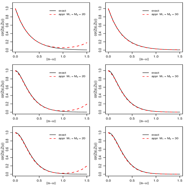
Figure 2: Plots of the correlation functions of $Z(\cdot)$ (solid black lines) and $T_{M_{1},M_{2}}(\cdot)$ (broken red lines) corresponding to the isotropic Matérn correlation functions with $\vartheta=0.4$ and $\nu=0.5,1.5$ and $2.5$ (top, middle and bottom panels). In all $\Delta=0.1$ was used.

3.2 Approximate Integrated Likelihood

Let $\tilde{\boldsymbol{\Sigma}}_{\vartheta}\coloneqq{\rm var}(\tilde{\boldsymbol{z}})$. Although $\tilde{\boldsymbol{\Sigma}}_{\vartheta}\approx\boldsymbol{H}_{1}\boldsymbol{G}_{\vartheta}\boldsymbol{H}_{1}^{\top}$ when $M_{1}$ and $M_{2}$ are both large, replacing the former matrix with the latter in (2.1) or (2.2) does not generally result in a computationally convenient approximation of the integrated likelihood of $\theta$. So we explore the alternative route of computing reference priors from the likelihood of a special linear combination of $\tilde{\boldsymbol{z}}$, somewhat similar to what is done for estimation of variance components using restricted likelihoods. In all that follows, the aliased spectral density $f^{\Delta}_{\vartheta}(\mbox{\boldmath$\omega$})$ is approximated by truncating the series (3.2) so that only the terms for which $\max\{|l_{1}|,|l_{2}|\}\leq T$ are retained, for some $T\in{\mathbb{N}}$; this approximation is denoted by $\tilde{f}^{\Delta}_{\vartheta}(\mbox{\boldmath$\omega$})$. Extensive numerical exploration shows that when $T$ is chosen in the range 3–6, the contribution of additional terms in (3.2) is negligible, so $\tilde{f}^{\Delta}_{\vartheta}(\mbox{\boldmath$\omega$})$ is not sensitive to $T$; see Section 5.

Let $\boldsymbol{L}_{1}\coloneqq\boldsymbol{H}_{1}(\boldsymbol{H}_{1}^{\top}\boldsymbol{H}_{1})^{-1/2}$, where $\boldsymbol{H}_{1}$ is the matrix defined above, and $\boldsymbol{V}_{1}\coloneqq\boldsymbol{L}_{1}^{\top}\tilde{\boldsymbol{z}}$. Because of the regular arrangements of locations ${\mbox{\boldmath$u$}}_{i,j}$ and frequencies $\mbox{\boldmath$\omega$}_{m_{1},m_{2}}$, and the orthogonality properties of cosines and sines, it holds that

$$\boldsymbol{H}^{\top}{\bf 1}_{M}={\bf 0}_{M-1}\quad{\rm and}\quad\boldsymbol{H}_{1}^{\top}\boldsymbol{H}_{1}=M{\rm diag}\big{(}1,1,1,1,\underbrace{2,\ldots,2}_{\tiny\mbox{$M-4$ times}}\big{)};$$ (3.5)

(see for instance Bose et al. (2018, Appendix E)). From these facts, direct calculation shows that

$$\boldsymbol{V}_{1}\stackrel{{\scriptstyle{\scriptsize\rm approx}}}{{\sim}}{\rm N}\left(\boldsymbol{X}_{1}\mbox{\boldmath$\beta$},\sigma^{2}\tilde{\boldsymbol{\Lambda}}_{\vartheta}\right),$$ (3.6)

where $\boldsymbol{X}_{1}:=\boldsymbol{L}_{1}^{\top}\tilde{\boldsymbol{X}}$ is an $M\times p$ matrix with full rank $p$, and $\tilde{\boldsymbol{\Lambda}}_{\vartheta}$ is the diagonal matrix

$$\tilde{\boldsymbol{\Lambda}}_{\vartheta} =c_{\Delta}{\rm diag}\Big{(}\big{(}\tilde{f}^{\Delta}_{\vartheta}(\mbox{\boldmath$\omega$}_{m_{1},m_{2}}):(m_{1},m_{2})\in I_{\rm C}\big{)}^{\top},\ \big{(}\tilde{f}^{\Delta}_{\vartheta}(\mbox{\boldmath$\omega$}_{m_{1},m_{2}}):(m_{1},m_{2})\in I\big{)}^{\top},$$

$$\hskip 170.71652pt\big{(}\tilde{f}^{\Delta}_{\vartheta}(\mbox{\boldmath$\omega$}_{m_{1},m_{2}}):(m_{1},m_{2})\in I\big{)}^{\top}\Big{)}.$$ (3.7)

Although the components of $\boldsymbol{V}_{1}$ are not error contrasts in general, its approximate covariance matrix is substantially simpler (diagonal) than that of $\tilde{\boldsymbol{z}}$. So applying the reference prior algorithm described in Section 2.1 based on the likelihood of $\boldsymbol{V}_{1}$ will result in substantial simplifications. Section 5 shows that this route delivers close approximations to reference priors when $\mathcal{U}_{M}$ is tuned to the features of the sampling design $\mathcal{S}_{n}$.

An important special case is that of models with constant mean function, i.e., when $p=1$. In this case, $\boldsymbol{X}_{1}\beta_{1}=(\sqrt{M}\beta_{1},\;{\bf 0}_{M-1}^{\top})^{\top}$ so the last $M-1$ components of $\boldsymbol{V}_{1}$ form a set of $M-1$ linearly independent error contrasts of $\tilde{\boldsymbol{z}}$. As a result, direct calculation from (3.6) shows that the restricted log–likelihood function of $\theta$ based on $\tilde{\boldsymbol{z}}$ is, up to an additive constant, approximately equal to

$$l^{\rm AI}(\mbox{\boldmath$\theta$};\tilde{\boldsymbol{z}})\;=\;-\frac{1}{2}\sum_{j=1}^{M-1}\left(\log\Big{(}c_{\Delta}\sigma^{2}\tilde{f}^{\Delta}_{\vartheta}(\mbox{\boldmath$\omega$}_{j})\Big{)}+\frac{V_{j}^{2}}{c_{\Delta}\sigma^{2}\tilde{f}^{\Delta}_{\vartheta}(\mbox{\boldmath$\omega$}_{j})}\right),$$ (3.8)

where $\mbox{\boldmath$\omega$}_{j}$ is a re–indexing of the frequencies $\mbox{\boldmath$\omega$}_{m_{1},m_{2}}$ appearing in (3.7), with $\mbox{\boldmath$\omega$}_{0,0}$ removed, and $V_{1},\ldots,V_{M-1}$ are the last $M-1$ components of $\boldsymbol{V}_{1}$. In this case, even more substantial simplifications accrue in the computation of approximate reference priors since (3.8) is a matrix–free expression and the required expectations are simplified as the $V_{j}$s are independent with $V_{j}^{2}\stackrel{{\scriptstyle{\tiny\rm approx}}}{{\sim}}{\rm Gamma}\big{(}1/2,2\sigma^{2}c_{\Delta}\tilde{f}^{\Delta}_{\vartheta}(\mbox{\boldmath$\omega$}_{j})\big{)}$ (shape–scale parametrization). Additionally, for Matérn correlation functions, differentiation with respect to the range parameter $\vartheta$ is simplified since $l^{\rm AI}(\mbox{\boldmath$\theta$};\tilde{\boldsymbol{z}})$ is devoid of Bessel functions. Finally, Harville (1974) showed that the integrated likelihood $L^{\rm I}(\mbox{\boldmath$\theta$};\tilde{\boldsymbol{z}})$ is proportional to the restricted likelihood function of $\theta$ based on a set of error contrasts $\boldsymbol{A}^{\top}\tilde{\boldsymbol{z}}$ when $\boldsymbol{A}$ satisfies $\boldsymbol{A}^{\top}\boldsymbol{A}=\boldsymbol{I}_{M-1}$ and $\boldsymbol{A}\boldsymbol{A}^{\top}=\boldsymbol{I}_{M}-\frac{1}{M}{\bf 1}_{M}{\bf 1}_{M}^{\top}$. Since the ratio of the restricted likelihood functions of $\theta$ based on any two sets of linearly independent error contrasts does not depend on $\theta$, it follows that $\log L^{\rm I}(\mbox{\boldmath$\theta$};\tilde{\boldsymbol{z}})$ is, up to an additive constant, approximately equal to (3.8).

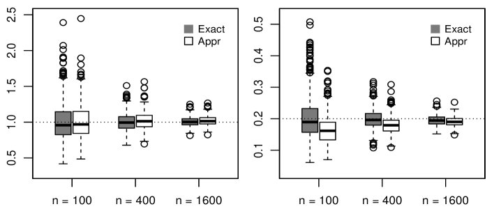
Figure 3: Boxplot of exact and approximate REML estimates of $\sigma^{2}$ (left) and $\vartheta$ (right) for different sample sizes. The true model is a Gaussian random field with mean 0 and Matérn covariance function with parameters $\sigma^{2}=1$, $\vartheta=0.2$ and $\nu=0.5$.

Consider situations where the sampling design is regular, and the mean function is constant. By setting $M=n$ and $\mathcal{U}_{M}=\mathcal{S}_{n}$, so $\tilde{\boldsymbol{z}}=\boldsymbol{z}$, restricted maximum likelihood (REML) estimates of the covariance parameters can be approximated by maximizing (3.8). This is appealing when the sample size is large, since in this case the computation of exact REML estimates (obtained by maximizing (2.1) or (2.2)) may be very time–consuming or even unfeasible. We ran a small simulation to compare the sampling distributions of exact and approximate REML estimators. For each sample size $n=100,400$ and $1600$, the Gaussian random field with mean 0 and Matérn covariance function with $\sigma^{2}=1$, $\vartheta=0.2$ and $\nu=0.5$ was simulated $500$ times over the $\sqrt{n}\;\times\sqrt{n}$ regular lattice with $\Delta=0.1$, and for each simulated data set exact and approximate REML estimates of $\mbox{\boldmath$\theta$}=(\sigma^{2},\vartheta)$ were computed, assuming $\nu$ known. Figure 3 displays boxplots from the REML estimates of $\sigma^{2}$ (left) and $\vartheta$ (right). This suggests the sampling distributions of exact and approximate REML estimators of $\sigma^{2}$ are close, even in small samples. On the other hand, the sampling distributions of exact and approximate REML estimators of $\vartheta$ are close only for large samples. For small samples, approximate REML estimators of $\vartheta$ are (downward) biased and less variable than their exact counterparts. The same behaviours were observed for other model settings (not shown). In terms of computational effort, when $n=1600$ the computation of exact REML estimates took 597 seconds on average, while the computation of approximate REML estimates took 1.71 seconds (in this work, computation time were reported using a MacBook Pro with 2.3 GHz Intel Core i9 processor under the R programming language).

4 Approximate Reference Priors

The derivation of the approximate reference prior, to be denoted as $\pi^{\rm AR}(\vartheta)$, proceeds as follows. Rather than using the exact integrated likelihood, (2.1) or (2.2), based on the data $\boldsymbol{z}$ measured at $\mathcal{S}_{n}$, we use the approximate integrated likelihood derived from the potential summary (3.6) measured at $\mathcal{U}_{M}$. This summary has a substantially simpler (diagonal) covariance matrix which, for the Matérn and other families, is also devoid of special functions. This makes the evaluation and analysis of the resulting approximate reference prior much more manageable than those of the exact reference prior. In what follows, we state expressions for the approximate reference priors and establish the propriety of the corresponding approximate reference posteriors. In these it is assumed that the covariates, if any, are available everywhere.

Theorem 1 (Approximate Reference Prior).

The approximate reference prior of $(\mbox{\boldmath$\beta$},\sigma^{2},\vartheta)$ derived from (3.6) is given by $\pi^{\rm AR}(\mbox{\boldmath$\beta$},\sigma^{2},\vartheta)\propto\frac{\pi^{\rm AR}(\vartheta)}{\sigma^{2}}$, where

$$\pi^{\rm AR}(\vartheta)\propto\left\{{\rm tr}\left[\left\{\left(\frac{\partial}{\partial\vartheta}\tilde{\boldsymbol{\Lambda}}_{\vartheta}\right)\tilde{\boldsymbol{Q}}_{\vartheta}\right\}^{2}\right]-\frac{1}{M-p}\left[{\rm tr}\left\{\left(\frac{\partial}{\partial\vartheta}\tilde{\boldsymbol{\Lambda}}_{\vartheta}\right)\tilde{\boldsymbol{Q}}_{\vartheta}\right\}\right]^{2}\right\}^{\frac{1}{2}},$$ (4.1)

with $\tilde{\boldsymbol{\Lambda}}_{\vartheta}$ defined in (3.7) and $\tilde{\boldsymbol{Q}}_{\vartheta}:=\tilde{\boldsymbol{\Lambda}}_{\vartheta}^{-1}-\tilde{\boldsymbol{\Lambda}}_{\vartheta}^{-1}\boldsymbol{X}_{1}(\boldsymbol{X}_{1}^{\top}\tilde{\boldsymbol{\Lambda}}_{\vartheta}^{-1}\boldsymbol{X}_{1})^{-1}\boldsymbol{X}_{1}^{\top}\tilde{\boldsymbol{\Lambda}}_{\vartheta}^{-1}$.

Proof. The result follows from (2.4) by replacing $\boldsymbol{X}$ with $\boldsymbol{X}_{1}$ and $\boldsymbol{\Sigma}_{\vartheta}$ with $\tilde{\boldsymbol{\Lambda}}_{\vartheta}$.

Note that $\tilde{\boldsymbol{\Lambda}}_{\vartheta}$ is a diagonal matrix so its inverse is easy to compute. The computation of $\tilde{\boldsymbol{Q}}_{\vartheta}$ only involves the inversion of the (small) $p\times p$ matrix $\boldsymbol{X}_{1}^{\top}\tilde{\boldsymbol{\Lambda}}_{\vartheta}^{-1}\boldsymbol{X}_{1}$, where the matrix $\boldsymbol{X}_{1}$ needs to be computed only once since $\boldsymbol{H}_{1}$ is fixed. The diagonal elements of the diagonal matrix $(\partial\tilde{\boldsymbol{\Lambda}}_{\vartheta}/\partial\vartheta)\tilde{\boldsymbol{\Lambda}}_{\vartheta}^{-1}$, namely $(\partial/\partial\vartheta)\log\tilde{f}^{\Delta}_{\vartheta}(\mbox{\boldmath$\omega$}_{m_{1},m_{2}})$, have a closed–form expression which for the Matérn and other models is devoid of special functions. As a result, the computation and analysis of $\pi^{\rm AR}(\vartheta)$ is substantially simpler than that of $\pi^{\rm R}(\vartheta)$. Note $\pi^{\rm AR}(\vartheta)$ could also be obtained from (2.5), but the resulting expression does not afford computational savings, so it is omitted.

An important special case of the above result occurs when the mean function is constant, in which case the approximate reference prior of $\vartheta$ takes an even simpler matrix–free form.

Corollary 1 (Constant Mean Case).

Consider models with constant mean function. In this case, the approximate reference prior of $(\beta_{1},\sigma^{2},\vartheta)$ is $\pi^{\rm AR}(\beta_{1},\sigma^{2},\vartheta)\propto\frac{\pi^{\rm AR}(\vartheta)}{\sigma^{2}}$, where

$$\pi^{\rm AR}(\vartheta)\propto\left\{\sum_{j=1}^{M-1}\left(\frac{\partial}{\partial\vartheta}\log\tilde{f}^{\Delta}_{\vartheta}(\mbox{\boldmath$\omega$}_{j})\right)^{2}-\frac{1}{M-1}\bigg{(}\sum_{j=1}^{M-1}\frac{\partial}{\partial\vartheta}\log\tilde{f}^{\Delta}_{\vartheta}(\mbox{\boldmath$\omega$}_{j})\bigg{)}^{2}\right\}^{\frac{1}{2}},$$ (4.2)

where $\mbox{\boldmath$\omega$}_{j}$ is a re–indexing of the frequencies $\mbox{\boldmath$\omega$}_{m_{1},m_{2}}$ in (3.7), with $\mbox{\boldmath$\omega$}_{0,0}=(0,0)^{\top}$ removed.

Proof. See the Appendix. This result can also be obtained by applying the last step of the reference prior algorithm to the approximate log–integrated likelihood (3.8) (not shown).

It should be noted that, because of isotropy, the (unnormalized) prior $\pi^{\rm AR}(\vartheta)$ can also be computed by including in the sum (4.2) all frequencies in $\mathcal{W}_{M}-\{\mbox{\boldmath$\omega$}_{0,0}\}$, which is proportional to the sample standard deviation of the derivative w.r.t. the range parameter of the log aliased spectral density evaluated at these frequencies.

To establish the propriety behaviour of the approximate reference prior and posterior, we make the following assumptions about the second–order structure of $Z(\cdot)$:

1. The family of (normalized) spectral densities satisfies $\int_{{\mathbb{R}}^{2}}f_{\vartheta}(\mbox{\boldmath$\omega$})d\mbox{\boldmath$\omega$}=1$ for all $\vartheta>0$, and has the form

   $$f_{\vartheta}(\mbox{\boldmath$\omega$})=\frac{h_{1}(\mbox{\boldmath$\omega$})h_{2}(\vartheta)}{\big{(}\|\mbox{\boldmath$\omega$}\|^{2}+u(\vartheta)\big{)}^{a}},$$

   where

   $\bullet$ $h_{1}(\mbox{\boldmath$\omega$})$ is non–negative and continuous in ${\mathbb{R}}^{2}$, and $a$ is a constant.

   $\bullet$ $h_{2}(\vartheta)$ and $u(\vartheta)$ are positive and continuously differentiable functions on $(0,\infty)$.

   $\bullet$ $\lim_{\vartheta\rightarrow 0^{+}}f_{\vartheta}(\mbox{\boldmath$\omega$})=0$   (this implies $\lim_{\vartheta\rightarrow 0^{+}}K_{\vartheta}(r)={\bf 1}\{r=0\}$ (white noise)).

2. The correlation matrix $\boldsymbol{\Sigma}_{\vartheta}$ can be expressed as

   $$\boldsymbol{\Sigma}_{\vartheta}=\sum_{i=0}^{J}q_{i}(\vartheta)\boldsymbol{D}^{(i)}+\boldsymbol{R}(\vartheta),\quad\quad{\rm as}\ \ \vartheta\rightarrow\infty,$$

   where $J\in{\mathbb{N}}$, the $q_{i}(\vartheta)$s are continuous functions on $(0,\infty)$, the $\boldsymbol{D}^{(i)}$s are fixed symmetric matrices satisfying $\cap_{i=0}^{J}{\rm Ker}(\boldsymbol{D}^{(i)})=\{{\bf 0}_{n}\}$, and $\boldsymbol{R}(\vartheta)$ is a function from $(0,\infty)$ to the space of $n\times n$ real matrices.

Theorem 2 (Propriety).

Assume the mean function $\mu({\bf s})$ has an intercept (so $f_{1}({\bf s})\equiv 1$).

(a) If $f_{\vartheta}(\mbox{\boldmath$\omega$})$ satisfies assumption (A1), then the approximate marginal reference prior $\pi^{\rm AR}(\vartheta)$ in (4.1) is a continuous function satisfying

$$\pi^{\rm AR}(\vartheta)=O\left(|u^{\prime}(\vartheta)|\land\frac{|u^{\prime}(\vartheta)|}{u^{2}(\vartheta)}\right),\;\;\;\text{as}\;\;\vartheta\to 0^{+}\;\;{\rm and}\;\;\vartheta\to\infty,$$ (4.3)

where $x\land y\coloneqq\min\{x,y\}$. So, if $|u^{\prime}(\vartheta)|\land|u^{\prime}(\vartheta)|u(\vartheta)^{-2}$ is integrable on $(0,\infty)$, $\pi^{\rm AR}(\vartheta)$ is proper.

(b) If the second–order structure of $Z(\cdot)$ satisfies assumptions (A1) and (A2), then the approximate reference posterior distribution based on the observed data, $\pi^{\rm AR}(\mbox{\boldmath$\beta$},\sigma^{2},\vartheta~{}|~{}\boldsymbol{z})\propto L(\mbox{\boldmath$\beta$},\sigma^{2},\vartheta;\boldsymbol{z})\pi^{\rm AR}(\mbox{\boldmath$\beta$},\sigma^{2},\vartheta)$, is proper.

Proof. See the Appendix.

Corollary 2 (Propriety for the Matérn Family).

Consider a model determined by a mean function $\mu({\bf s})$ with an intercept and the Matérn family of (normalized) spectral densities (3.1). Then, $\pi^{\rm AR}(\vartheta)$ is integrable on $(0,\infty)$ and $\pi^{\rm AR}(\mbox{\boldmath$\beta$},\sigma^{2},\vartheta~{}|~{}\boldsymbol{z})$ is proper.

Proof. The Matérn family (3.1) clearly satisfies (A1), with $h_{1}(\mbox{\boldmath$\omega$})=\Gamma(\nu+1)(4\nu)^{\nu}/\pi\Gamma(\nu)$, $h_{2}(\vartheta)=\vartheta^{-2\nu}$, $u(\vartheta)=4\nu/{\vartheta^{2}}$ and $a=\nu+1$. Then

$$|u^{\prime}(\vartheta)|\land\frac{|u^{\prime}(\vartheta)|}{u^{2}(\vartheta)}\ =\ \frac{8\nu}{\vartheta^{3}}\land\frac{\vartheta}{2\nu}\ =\ \begin{cases}o(1),&\text{as}\ \vartheta\to 0^{+}\\ O(\vartheta^{-3}),&\text{as}\ \vartheta\to\infty\end{cases},$$

is integrable on $(0,\infty)$, so by Theorem 2(a) $\pi^{\rm AR}(\vartheta)$ is proper. Also, it was shown in Muré (2021) that the Matérn family (3.1) satisfies (A2), so the propriety of $\pi^{\rm AR}(\mbox{\boldmath$\beta$},\sigma^{2},\vartheta~{}|~{}\boldsymbol{z})$ follows from Theorem 2(b).

The preceding results provide a theoretical justification for using the approximate reference prior under either constant mean or non–constant mean model with a common intercept. Note that, in general, $\pi^{\rm AR}(\vartheta)$ is proper and its tail rate as $\vartheta\to\infty$ is the same regardless of the mean function and degree of smoothness of the random field. On the other hand, Muré (2021) showed that, in general, $\pi^{\rm R}(\vartheta)=O(1/\vartheta)$ as $\vartheta\rightarrow\infty$, and this tail behaviour is sharp for some models. Muré also showed that for some special models, other tail behaviours hold; (Muré, 2021, Appendix B). Consequently, $\pi^{\rm R}(\vartheta)$ is not always proper and the proposed use of (exact) reference priors and Bayes factors discussed in Berger et al. (2001, Section 6) for selecting smoothness in correlation families are not valid. In contrast, $\pi^{\rm AR}(\vartheta)$ can always be used for this purpose; this is illustrated in Section 6.

The marginal prior $\pi^{\rm AR}(\vartheta)$ depends on the tuning constants $M_{1}$, $M_{2}$ and $\Delta$ that need to be tuned to the sampling design $\mathcal{S}_{n}$. Since these have specific interpretations in terms of the spectral approximation, their selection is more straightforward than using a subjectively chosen prior, for example, an inverse gamma prior, since it is unclear how to select the hyperparameters; this is discussed in Section 5.

Discussion. Assumption (A1) is satisfied by several families of spectral densities proposed in the literature, after a reparametrization if needed. In addition to the Matérn family, the family proposed by Laga and Kleiber (2017) (assuming their parameters b and $\xi$ are known), is of this form with $h_{1}(\mbox{\boldmath$\omega$})=({\rm b}^{2}+\|\mbox{\boldmath$\omega$}\|^{2})^{\xi}$, $h_{2}(\vartheta)\propto 1$, $u(\vartheta)=1/\vartheta^{2}$ and $a=\nu+1$. Also, some of the families of spectral densities studied in Vecchia (1985) and Jones and Vecchia (1993) are of this form, after they are suitably parametrized.

Assumption (A2) is a more general expansion than that in (2.9). The latter occurs when $J=1$, $q_{0}(\vartheta)=1$, $\boldsymbol{D}^{(0)}={\bf 1}_{n}{\bf 1}_{n}^{\top}$, $q_{1}(\vartheta)=q(\vartheta)$, $\boldsymbol{D}^{(1)}=\boldsymbol{D}$ and $\boldsymbol{R}(\vartheta)=o(q(\vartheta))$, with $q(\vartheta)$ and $\boldsymbol{D}$ defined circa (2.9). When $\boldsymbol{D}$ is non–singular, ${\rm Ker}({\bf 1}_{n}{\bf 1}_{n}^{\top})\cap{\rm Ker}(\boldsymbol{D})=\{{\bf 0}_{n}\}$ clearly holds. Likewise, a sufficient (but not necessary) condition for $\cap_{i=0}^{J}{\rm Ker}(\boldsymbol{D}^{(i)})=\{{\bf 0}_{n}\}$ to hold is that at least one matrix $\boldsymbol{D}^{(i)}$ is non–singular. Muré (2021) checked that assumption (A2) holds for several commonly used families of covariance functions, including the Matérn family.

5 Numerical Studies

In this section, we conduct numerical studies to explore how close the marginal priors $\pi^{\rm R}(\vartheta)$ and $\pi^{\rm AR}(\vartheta)$ are for various sampling designs and model features, and provide empirical guidelines for the selection of the tuning constants $M_{1},M_{2}$ and $\Delta$. Additionally, we also compare the computational efforts for their computation.

We consider two regular designs, a $10\times 10$ equally spaced grid in $[0,1]^{2}$ and a $20\times 20$ equally spaced grid in $[0,2]^{2}$, as well as three irregular sampling designs in $[0,1]^{2}$ of size $n=100$, to be described below. For the mean function we consider $\mu({\bf s})=1$ and $\mu({\bf s})=0.15-0.65x-0.1y+0.9x^{2}-xy+1.2y^{2}$, with ${\bf s}=(x,y)$, and for the covariance function we consider the isotropic Matérn model (1.1) with $\nu=0.5,1.5$ and $2.5$. In all cases the approximate reference priors are computed with $\tilde{f}^{\Delta}_{\vartheta}(\mbox{\boldmath$\omega$}_{j})$ obtained by truncating the series (3.2) so that only the terms with $\max\{|l_{1}|,|l_{2}|\}\leq 5$ are retained. These approximate reference priors show no sensitivity to the truncation point.

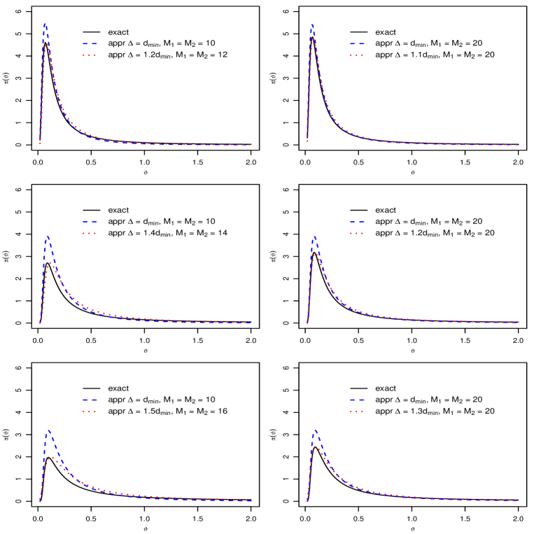
Figure 4: Marginal densities of the exact and approximate reference priors of $\vartheta$ for the constant mean models under different sample designs and covariance smoothness. Left: $10\times 10$ equally spaced grid in $[0,1]^{2}$. Right: $20\times 20$ equally spaced grid in $[0,2]^{2}$. From top to bottom: $\nu=0.5,1.5$ and $2.5$.

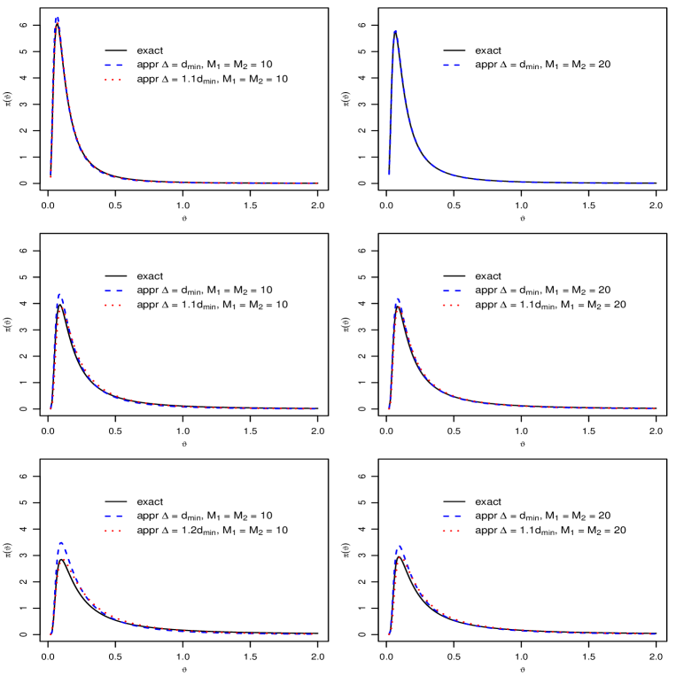
Figure 5: Marginal densities of the exact and approximate reference priors of $\vartheta$ for the non–constant mean models under different sample designs and covariance smoothness. Left: $10\times 10$ equally spaced grid in $[0,1]^{2}$. Right: $20\times 20$ equally spaced grid in $[0,2]^{2}$. From top to bottom: $\nu=0.5,1.5$ and $2.5$.

Figure 4 displays the (normalized) reference priors of $\vartheta$ based on the regular designs for models with constant mean. The left panels are the priors based on the grid in $[0,1]^{2}$, the right panels are the priors based on the grid in $[0,2]^{2}$, and the top, middle and bottom panels are the priors obtained when $\nu=0.5,1.5$ and $2.5$, respectively. The solid black curves are exact reference priors, and the broken colored curves are approximate reference priors. As the default choice to compute $\pi^{\rm AR}(\vartheta)$ we use $\mathcal{U}_{M}=\mathcal{S}_{n}$, i.e., we set $M_{1}=M_{2}=\sqrt{n}$ and $\Delta=d_{\min}$, the distance between adjacent sampling locations. The resulting approximate reference priors (broken blue curves) display the same shapes as the exact reference priors, both having about the same mode, but do not provide a very close approximation in general. But the approximation improves substantially when $M_{1}$, $M_{2}$ and/or $\Delta$ are tuned. Figure 4 also displays approximate reference priors (broken red curves) obtained by setting $M_{1}=M_{2}\geq\sqrt{n}$ and $\Delta>d_{\min}$ at values indicated in the legends. Now the approximate reference priors provide close approximations. Less tuning is needed for the larger sample size, as using the default $M_{1}=M_{2}=\sqrt{n}$ and only tuning $\Delta$ results in good approximations; the required tuned value of $\Delta$ increases with the smoothness. Additionally, and in agreement with part (b) of Lemma 1, the approximations in the right panels are closer to their exact counterparts than the ones in the left panels since $M_{1}$ and $M_{2}$ are larger for the former.

Figure 5 displays the (normalized) reference priors of $\vartheta$ based on the regular designs for models with non–constant mean, with the same layout used in Figure 4. The behaviours and conclusions are essentially the same as those in Figure 4. But now the approximate reference priors are even closer to their exact counterparts, and the default choice provides even closer approximations. Moreover, setting $M_{1}=M_{2}=\sqrt{n}$ and only tuning $\Delta$ results in good approximations also for the small sample size, and even no adjustment at all (i.e., also setting $\Delta=d_{\min}$) may provide a good approximation when the sample size is large and the process is not smooth.

The results in Figures 4 and 5, as well as additional numerical explorations (not shown), suggest that, as a rule of thumb, for sampling designs that are small regular grids, the adjustment involves setting $M_{1}$ (for simplicity $M_{2}=M_{1}$) and $\Delta$ to values 10–40% larger than $\sqrt{n}$ and $d_{\min}$, respectively. For larger regular grids it may suffice to set $M_{1}=\sqrt{n}$ and only adjust $\Delta$ to a value about 10% larger than $d_{\min}$. Overall, the approximate reference priors are more sensitive to $\Delta$ than to $M_{1}$ (the Supplementary Materials provide an illustration of this fact). Finally, for regular grids with similar $d_{\min}$, both the exact and the approximate reference priors of $\vartheta$ are more sensitivity to $\nu$ than to $n$ or $M_{1}$, and the approximations seem to be closer for non–smooth random fields.

Figure 6: Left: Three different sampling designs in $[0,1]^{2}$. Right: Corresponding marginal densities of the exact and approximate reference priors of $\vartheta$ under constant mean model when $\nu=0.5$.

Next we consider three irregular sampling designs in $[0,1]^{2}$ of size $n=100$: an incomplete $14\times 14$ regular grid, a hybrid design generated by the method proposed in Bachoc (2014), with $\epsilon=0.499$, and a random sample from the ${\rm unif}((0,1)^{2})$ distribution. These designs are displayed in Figure 6 (left panels). Figure 6 (right panels) displays the exact and approximate reference priors of $\vartheta$ (solid black and broken red curves, respectively) based on these irregular designs for the model with constant mean and Matérn correlation with $\nu=0.5$. The approximate reference priors can still provide satisfactory approximations for practical purposes, although the discrepancy between the two priors increases with the degree of irregularity of the design. The results for models with a non–constant mean and other degrees of smoothness displayed similar behaviours (not shown). The tuning of $M_{1}$ and $M_{2}$ was done similarly as described above for regular designs, but now $\Delta$ is selected based on the distances to the nearest neighbors, $d_{i}=\min\{\|{\bf s}_{i}-{\bf s}_{j}\|:j\neq i\}$. It was empirically found that setting $\Delta$ at a value between the 75 to 95 percentiles of $\{d_{i}\}_{i=1}^{n}$ provides reasonable approximations under the above designs. Overall, the numerical explorations reported in Figures 4–6 indicate that approximate reference priors, after properly tuned, provide satisfactory approximations to exact reference priors for a variety of sampling designs and models. For large sample sizes when an approximation is most needed, the tuning simplifies as we can set $M_{1}=M_{2}\approx\sqrt{n}$ and only select $\Delta$ using the aformentioned guideline. The Supplementary Materials provide a more detailed comparison of the tail behaviour of these priors, showing that approximate reference priors tend to have lighter tails than their exact counterparts (the text after Corollary 2 explains the reason for this behaviour).

Table 1: Computational time (in seconds) for $500$ evaluations of the exact and approximate reference priors of $\vartheta$ for regular grid sampling designs of different sample sizes and several model features.

$\nu$	$p$	Reference Prior		$n=100$	$n=400$	$n=1600$	$n=10000$
$0.5$	$1$	Exact		$1.18$	$41.56$	$2652.75$	–
		Approximate		$0.21$	$0.87$	$2.05$	$10.21$
	$6$	Exact		$2.48$	$61.49$	$4098.96$	–
		Approximate		$0.68$	$2.62$	$32.08$	$712.09$
$1$	$1$	Exact		$3.80$	$81.46$	$3459.14$	–
		Approximate		$0.14$	$0.77$	$2.10$	$9.69$
	$6$	Exact		$8.01$	$104.44$	$5047.18$	–
		Approximate		$0.81$	$3.04$	$29.94$	$694.33$

To discuss the computational complexity of exact and approximate reference priors, we consider for simplicity a regular grid $\sqrt{n}\;\times\sqrt{n}$ sampling design and use $M=n$. The computation of the exact reference prior $\pi^{\rm R}(\vartheta)$ in (2.4) requires $O(M^{3})$ operations due to the need of numerically invert $\boldsymbol{\Sigma}_{\vartheta}$. On the other hand, for processes with constant mean the computation of the approximate reference prior $\pi^{\rm AR}(\vartheta)$ in (4.2) only requires $O(M)$ operations. For processes with a non–constant mean function the computation of $\pi^{\rm AR}(\vartheta)$ in (4.1) requires $O(M^{2})$ operations (and does not involve the evaluation of special functions). This is so due to the need to compute the matrix $\boldsymbol{X}_{1}$ (only once), with $O(M^{2})$ computational complexity, and then computing $\boldsymbol{X}_{1}(\boldsymbol{X}_{1}^{\top}\tilde{\boldsymbol{\Lambda}}_{\vartheta}^{-1}\boldsymbol{X}_{1})^{-1}\boldsymbol{X}_{1}^{\top}\tilde{\boldsymbol{\Lambda}}_{\vartheta}^{-1}$, which also has $O(M^{2})$ computational complexity.

Table 1 reports the timings for 500 evaluations of both marginal reference priors of $\vartheta$ under regular $\sqrt{n}\;\times\sqrt{n}$ sampling designs for models with constant and non–constant mean functions and Matérn covariance functions with $\nu=0.5$ and $1$. For the evaluation of the approximate reference prior we used $\Delta=0.1$ and $M=n$. The evaluation of approximate reference priors is between one and two orders of magnitude faster than that of exact reference priors, and the computational time gap increases substantially with sample size. In particular, the computation of exact reference priors becomes computationally unfeasible when $n=10000$.

The Supplementary Materials report results from a simulation study to compare frequentist properties of Bayesian procedures based on approximate and exact reference priors (under two types of the sampling designs), as well as frequentist properties of a purely likelihood–based procedure (under the regular lattice design for illustrative purposes). The results suggest that the credible intervals for the covariance parameters based on these two priors have similar and satisfactory frequentist coverage, and their expected lengths are also about the same in most case scenarios. In addition, the mean absolute errors of the Bayesian estimators of the range parameter based on these two priors are about the same, and these are smaller than the mean absolute error of maximum likelihood estimators.

6 Example

We illustrate the application of default Bayesian analysis based on exact and approximate reference priors with a data set analyzed by Diggle et al. (2010), available in the R package PrevMap. The data set, which came about in the monitoring of lead pollution in Galicia, northern Spain, consists of measurements of lead concentrations in moss samples (in micrograms per gram dry weight). Data from two survey times were analyzed by Diggle et al. (2010), one in October 1997 and the other in July 2000. Here we use the July 2000 data, since the 1997 data were collected using a preferential sampling design. The analysis uses the log–transformation of the original measurements to eliminate their variance–mean relationship, which renders the homoscedastic Gaussian assumption appropriate. A summary of the data is plotted in Figure 7 (left), showing $132$ sampling locations where the unit of distance is 100 km.

There are no covariates available and an exploratory analysis reveals no apparent spatial trend, so the mean function is assumed constant. Figure 7 (right) displays the empirical semivariogram and the fitted (by least squares) semivariogram function $0.21\big{(}1-\exp(-\sqrt{2}r/0.26)\big{)}$. This corresponds the Matérn covariance function (1.1) with $\nu=0.5$ which, except for a slight reparametrization, is the exponential semivariogram model used in Diggle et al. (2010). The fit appears appropriate for the data and suggests the data contain no measurement error (no nugget).

The sampling locations are close to form a regular grid, but they are not strictly aligned. For most sites, the distances to their nearest neighbors are similar (the $90$ percentile is about $15$ km and the maximum is $21$ km). To compute the approximate reference prior we set $M_{1}=M_{2}=16$ and $\Delta=0.2$, and $\tilde{f}^{\Delta}_{\vartheta}(\mbox{\boldmath$\omega$}_{j})$ is obtained by setting $\max\{|l_{1}|,|l_{2}|\}\leq 5$. Two Bayesian analyses were carried out based on the exact and approximate reference priors, where samples of size $10^{4}$ from the corresponding posteriors of $(\beta_{1},\sigma^{2},\vartheta)$ were simulated using the Monte Carlo algorithm described in the Supplementary Materials. The acceptance rate in the ratio–of–uniforms step was about $75\%$.

Figure 7: Left: Sampling locations of the lead concentration data in year 2000 and response bubble plot. Right: empirical semivariogram of the log–transformed lead concentration data and its least squares fit.

Figure 8 (left) displays the normalized exact and approximate reference priors of $\vartheta$, $\pi^{\rm R}(\vartheta)$ and $\pi^{\rm AR}(\vartheta)$, as well as their corresponding marginal posteriors. Both posterior distributions are quite close. Table 2 reports the Bayesian estimators of the model parameters and their corresponding $95\%$ highest posterior density (HPD) credible intervals based on both posteriors, showing that both inferences are essentially the same, as expected from the findings in Figure 8 (left). The modes of the two posteriors of $\vartheta$ are almost indistinguishable, and the estimates of $\beta_{1}$ and $\sigma^{2}$ are also very close. The analyses suggest that the approximate reference posterior has slightly lighter tails than the exact reference posterior, and as a result, the credible intervals from the former are slightly narrower.

Figure 8: Left: Densities of exact and approximate marginal reference priors and posteriors of $\vartheta$ for the lead concentration data. Right: Integrated likelihood of $\nu$ for the lead concentration data.

Table 2: Parameter estimates from the lead concentration data using exact and approximate reference priors. The estimate $\hat{\vartheta}$ is the posterior mode, $\hat{\sigma}^{2}$ is the posterior median and $\hat{\beta}_{1}$ is the posterior mean. The 95% credible intervals are the HPD.

Prior	$\hat{\beta}_{1}$	$\hat{\sigma}^{2}$	$\hat{\vartheta}$
	$(95\%~{}{\rm CI})$	$(95\%~{}{\rm CI})$	$(95\%~{}{\rm CI})$
Exact Reference Prior	$0.734$	$0.233$	$0.283$
	$(0.462,1.013)$	$(0.133,0.368)$	$(0.168,0.613)$
Approximate Reference Prior	$0.732$	$0.228$	$0.283$
	$(0.465,0.999)$	$(0.135,0.359)$	$(0.177,0.603)$

Note that the evaluation of the exponential covariance function and its derivative w.r.t. $\vartheta$ is devoid of Bessel functions. The computation time to draw $10^{4}$ posterior samples based on the approximate reference prior was about $78$ seconds, while the time to do the same task based on exact reference prior was $122$ seconds. In both the exact likelihood was used so the time difference is due to prior evaluations. For a Matérn model with $\nu\neq m+1/2$, where $m$ is a non–negative integer, the evaluation of the covariance function and its derivative w.r.t. $\vartheta$ involve Bessel functions, and in this case the computation time to draw a posterior sample of the same size jumps to $277$ seconds.

It is worth pointing out that the selection of the family of covariance functions is in general a difficult problem, and this is so in particular for the selection of the smoothness of the covariance family. Graphical summaries such as the one reported in Figure 7 (right) are often used to aid in this task, but they are of limited value due to the lack of measurements separated by small distances. Berger et al. (2001) suggested choosing the smoothness by inspecting its integrated likelihood. When the smoothness parameter is not assumed known, the (conditional) approximate reference prior is written as

$$\pi^{\rm AR}(\mbox{\boldmath$\beta$},\sigma^{2},\vartheta~{}|~{}\nu)=\frac{C(\nu)\pi^{\rm AR}(\vartheta~{}|~{}\nu)}{\sigma^{2}},$$

where $\pi^{\rm AR}(\vartheta~{}|~{}\nu)$ is given in (4.1), with the dependence on the smoothness parameter now being explicit, and $C(\nu)\coloneqq\big{(}\int_{0}^{\infty}\pi^{\rm AR}(\vartheta~{}|~{}\nu)d\vartheta\big{)}^{-1}$ is the normalizing constant. If $\boldsymbol{\vartheta}=(\vartheta,\nu)$ denotes the correlation parameters of the Matérn model, then the integrated likelihood of $\nu$ is given by

$$m(\boldsymbol{z}~{}|~{}\nu) =\int_{{\mathbb{R}}^{p}\times(0,\infty)^{2}}L(\mbox{\boldmath$\beta$},\sigma^{2},\vartheta,\nu;\boldsymbol{z})\pi^{\rm AR}(\mbox{\boldmath$\beta$},\sigma^{2},\vartheta~{}|~{}\nu)d\mbox{\boldmath$\beta$}d\sigma^{2}d\vartheta$$

$$\propto\int_{0}^{\infty}|\boldsymbol{\Sigma}_{\boldsymbol{\vartheta}}|^{-\frac{1}{2}}|\boldsymbol{X}^{\top}\boldsymbol{\Sigma}_{\boldsymbol{\vartheta}}^{-1}\boldsymbol{X}|^{-\frac{1}{2}}(S^{2}_{\boldsymbol{\vartheta}})^{-\frac{n-p}{2}}C(\nu)\pi^{\rm AR}(\vartheta~{}|~{}\nu)d\vartheta.$$

Note that this integrated likelihood is not well defined when the exact reference prior $\pi^{\rm R}(\vartheta~{}|~{}\nu)$ is used, since $C(\nu)$ does not exist for some $\nu\geq 1$, while it is well defined for the approximate reference prior; see Section 4. The smoothness parameter can now be chosen as the value that maximizes $m(\boldsymbol{z}~{}|~{}\nu)$. Figure 8 (right) displays the integrated likelihood of $\nu$ for the Galicia lead concentration data, showing that the choice $\nu=0.5$ was about right (the maximum occurs at $\nu=0.58$).

The Supplementary Materials report the results of data analysis for a (simulated) data set with different features from those of the above lead concentration data: an irregular sampling design of larger size and data from a smoother model. The results of the exact and approximate reference analyses were also in this case practically equivalent.

7 Conclusions

This work has derived and studied approximate reference priors for a class of geostatistical models, namely for isotropic Gaussian random fields whose covariance functions depend on unknown variance and range parameters. The methodology relies on a spectral approximation to the integrated likelihood of the covariance parameters, which produces close approximations to exact reference priors for a variety of sampling designs and model features.

The approximate reference priors derived in this work have a number of beneficial features that make them attractive for practical use. First, they can be evaluated in a fraction of the time required to evaluate exact reference priors because they do not involve inversion of large or ill–conditioned matrices nor the evaluation of special functions. For random fields with constant mean, the approximate reference prior has a simple matrix–free expression. Second, for many families of correlation functions, including the widely used Matérn family, the approximate marginal reference prior for the correlation parameter is proper, which is not always the case for models with smooth covariance function in the reference prior. This enables the use of approximate reference priors for covariance function selection using Bayes factors, as described in Berger et al. (2001). This is a very helpful property since very few tools are available for this purpose, and covariance selection is often done casually. Finally, results from simulation experiments reported in the Supplementary Materials show that inferences based on these approximate reference posteriors have satisfactory frequentist properties that are as good as those based on exact reference posteriors, and sometimes better than those based on purely likelihood–based inferences.

The proposed approximate reference prior depends on an auxiliary regular grid set up by the user. Tuning this grid allows the attainment of close approximations to exact reference priors for a variety of sampling designs and model features. The numerical studies in Section 5 provide useful guidelines for the setting of the tuning constants, and a default way for their determination will be investigated in future work. The approximation can be computed for random field models with explicit (normalized) spectral density that have the general form stated in Section 4. The isotropic Matérn family of correlation functions was used for illustration, but the methodology is equally applicable for other families, such as some families in Vecchia (1985), Jones and Vecchia (1993) and Laga and Kleiber (2017), possibly after a reparametrization and once some of their parameters are fixed.

It should be noted that the approximate reference priors derived here do not seem to converge to their exact counterparts in any strict mathematical sense. One reason is that exact reference priors depend on the sample size $n$, while approximate reference priors depend on $\Delta$, $M_{1}$ and $M_{2}$ that are in principle unrelated to $n$. Another reason is that, although it holds that ${\rm cov}\{T_{M_{1},M_{2}}({\bf u}_{i,j}),T_{M_{1},M_{2}}({\bf u}_{i^{\prime},j^{\prime}})\}\rightarrow\sigma^{2}K_{\vartheta}(||{\bf u}_{i,j}-{\bf u}_{i^{\prime},j^{\prime}}||)$ as $\min\{M_{1},M_{2}\}\to\infty$, a comparable result in the spectral domain may not hold due to the aliasing effect ($\Delta>0$ is fixed). Nevertheless, approximate reference priors provide useful working approximations, since they share the main properties of exact reference priors, and can be computed much faster in situations where the latter cannot.

The proposed methodology could be extended to models with more complex correlation functions. One possible extension is to approximate the reference priors derived in Kazianka and Pilz (2012) and Ren et al. (2012) for isotropic correlation functions with unknown range and nugget parameters, which would describe situations when geostatistical data contain measurement error. Another possible extension is to non–isotropic separable correlation functions that depend on several range parameters, which are commonly used in the analysis of data from computer experiments (Paulo, 2005). As pointed out by a reviewer, when the number of range parameters is large, the spectral approximation to the random field may not be as accurate for these models compared to the isotropic models, or may require a much larger $M$ to achieve a good approximation. For these models, Gu (2019) proposed an approximation to the (joint) reference prior of the range parameters aimed at matching the tail behaviours of their exact counterparts. A benefit of the latter approximation is that it can perform input selection, in the sense of identifying ‘inert inputs’. These extensions are currently being developed and will be reported elsewhere.

Finally, in recent years several methods have been proposed in the literature to approximate Gaussian likelihoods that include, but are not limited to, spectral approximations (Paciorek, 2007), composite likelihood approximations (Varin et al., 2011), low–rank approximations (Heaton et al., 2019) and Vecchia approximations (Katzfuss and Guinness, 2021). The combination of one of these with the approximate reference prior developed in this work would make it feasible to carry out default Bayesian analyses of large geostatistical data sets. This will be explored in future work.

Appendix: Proofs of the Main Results in Section 4

To prove the main results in Section 4, we use the following lemmas.

Lemma 2.

Let $\{x_{i}\}_{i=1}^{\infty}$ and $\{y_{i}\}_{i=1}^{\infty}$ be sequences of positive real numbers. If $\max\limits_{i}\left\{{x_{i}}/{y_{i}}\right\}=u<\infty$, then $\left(\sum_{i=1}^{\infty}x_{i}\right)/\left(\sum_{i=1}^{\infty}y_{i}\right)\leq u$.

Proof.

From the assumption follows that $x_{i}\leq uy_{i}$ for all $i$, so summing over all $i$ provides the result. ∎

Lemma 3.

Let $\boldsymbol{A}$ be an $n\times p$ real–valued matrix $(n>p)$ with rank $p-m>0$ and $m>0$, and $\boldsymbol{B}$ an $m\times p$ real–valued matrix with rank $m$ whose rows are linearly independent of the rows in $\boldsymbol{A}$. Then $\boldsymbol{B}(\boldsymbol{A}^{\top}\boldsymbol{A}+\boldsymbol{B}^{\top}\boldsymbol{B})^{-1}\boldsymbol{B}^{\top}=\boldsymbol{I}_{m}$

Proof.

See Chipman (1964, Theorem 1.1) or Mohammadi (2016, Lemma 1.1). ∎

Lemma 4.

Let $\boldsymbol{\Lambda}$ be a diagonal matrix with positive diagonal entries, $\boldsymbol{X}$ an $n\times p$ real–valued matrix with rank $p$ and $n>p$, and $\boldsymbol{P}=\boldsymbol{X}(\boldsymbol{X}^{\top}\boldsymbol{\Lambda}^{-1}\boldsymbol{X})^{-1}\boldsymbol{X}^{\top}\boldsymbol{\Lambda}^{-1}$ a projection matrix. If $\boldsymbol{P}_{ij}$ and $\boldsymbol{X}_{ij}$ are the $(i,j)^{th}$ entries of $\boldsymbol{P}$ and $\boldsymbol{X}$, respectively, then

(1) $\boldsymbol{P}_{ij}\boldsymbol{P}_{ji}\geq 0$ for all $i,j=1,\ldots,n$.

(2) The diagonal elements of $\boldsymbol{P}$ satisfies $0\leq\boldsymbol{P}_{ii}\leq 1$ for all $i=1,\ldots,n$.

(3) Let $\boldsymbol{X}_{(-1)}$ denote the matrix $\boldsymbol{X}$ with its first row removed and $\boldsymbol{0}_{n-1}$ the zero column vector of length $n-1$. If $\boldsymbol{0}_{n-1}$ is a column of $\boldsymbol{X}_{(-1)}$ and $\boldsymbol{X}_{11}\neq 0$, then $\boldsymbol{P}_{11}=1$.

Proof.

(1) This follows by noting that $\boldsymbol{X}(\boldsymbol{X}^{\top}\boldsymbol{\Lambda}^{-1}\boldsymbol{X})^{-1}\boldsymbol{X}^{\top}$ is symmetric and $\boldsymbol{\Lambda}^{-1}$ diagonal matrix with positive diagonal entries. (2) $\boldsymbol{P}_{ii}\geq 0$ follows from the fact that $(\boldsymbol{X}^{\top}\boldsymbol{\Lambda}^{-1}\boldsymbol{X})^{-1}$ is positive definite. And from $\boldsymbol{P}^{2}=\boldsymbol{P}$ and (1) we have that $\boldsymbol{P}_{ii}(1-\boldsymbol{P}_{ii})\geq 0$, so the result follows. (3) Let $\boldsymbol{X}^{*}=\boldsymbol{\Lambda}^{-\frac{1}{2}}\boldsymbol{X}$ and $\boldsymbol{P}^{*}=\boldsymbol{X}^{*}(\boldsymbol{X}^{*\top}\boldsymbol{X}^{*})^{-1}\boldsymbol{X}^{*\top}$, so it holds that $\boldsymbol{P}_{11}=\boldsymbol{P}^{*}_{11}$. From the inequalities ${\rm rank}(\boldsymbol{X}^{*})\leq\min\{{\rm rank}(\boldsymbol{\Lambda}^{-\frac{1}{2}}),{\rm rank}(\boldsymbol{X})\}\leq p$ and ${\rm rank}(\boldsymbol{X}^{*})\geq{\rm rank}(\boldsymbol{\Lambda}^{-\frac{1}{2}})+{\rm rank}(\boldsymbol{X})-n\geq p$ follow that ${\rm rank}(\boldsymbol{X}^{*})=p$. When $\boldsymbol{0}_{n-1}$ is a column of $\boldsymbol{X}_{(-1)}$, it is also a column of $\boldsymbol{X}^{*}_{(-1)}$, so ${\rm rank}(\boldsymbol{X}^{*}_{(-1)})=p-1$. Let $\boldsymbol{x}^{*}_{1}$ be the first row of $\boldsymbol{X}^{*}$, which is clearly linearly independent from the rows of $\boldsymbol{X}^{*}_{(-1)}$. Then by Lemma 3, $\boldsymbol{P}_{11}=\boldsymbol{P}_{11}^{*}=\boldsymbol{x}^{*}_{1}(\boldsymbol{X}_{(-1)}^{*\top}\boldsymbol{X}_{(-1)}^{*}+\boldsymbol{x}^{*\top}_{1}\boldsymbol{x}^{*}_{1})^{-1}\boldsymbol{x}^{*\top}_{1}=1$. ∎

Proof of Corollary 1.

It follows from (3.5) and direct calculation that

$$\tilde{\boldsymbol{Q}}_{\vartheta} =\frac{1}{c_{\Delta}}{\rm diag}\Big{(}\big{(}1/\tilde{f}^{\Delta}_{\vartheta}(\mbox{\boldmath$\omega$}_{m_{1},m_{2}}):(m_{1},m_{2})\in I_{\rm C}\big{)}^{\top},\ \big{(}1/\tilde{f}^{\Delta}_{\vartheta}(\mbox{\boldmath$\omega$}_{m_{1},m_{2}}):(m_{1},m_{2})\in I\big{)}^{\top},$$

$$\hskip 184.9429pt\big{(}1/\tilde{f}^{\Delta}_{\vartheta}(\mbox{\boldmath$\omega$}_{m_{1},m_{2}}):(m_{1},m_{2})\in I\big{)}^{\top}\Big{)}$$

$$\hskip 56.9055pt-\ \frac{\sqrt{M}}{c_{\Delta}}\Big{(}1/\tilde{f}^{\Delta}_{\vartheta}(\mbox{\boldmath$\omega$}_{0,0}),\;{\bf 0}_{M-1}^{\top}\Big{)}^{\top}\!\cdot\frac{c_{\Delta}\tilde{f}^{\Delta}_{\vartheta}(\mbox{\boldmath$\omega$}_{0,0})}{M}\cdot\frac{\sqrt{M}}{c_{\Delta}}\Big{(}1/\tilde{f}^{\Delta}_{\vartheta}(\mbox{\boldmath$\omega$}_{0,0}),\;{\bf 0}_{M-1}^{\top}\Big{)}$$

$$=\frac{1}{c_{\Delta}}{\rm diag}\Big{(}0,\big{(}1/\tilde{f}^{\Delta}_{\vartheta}(\mbox{\boldmath$\omega$}_{m_{1},m_{2}}):(m_{1},m_{2})\in I_{\rm C}-\{(0,0)^{\top}\}\big{)}^{\top},$$

$$\hskip 56.9055pt\big{(}1/\tilde{f}^{\Delta}_{\vartheta}(\mbox{\boldmath$\omega$}_{m_{1},m_{2}}):(m_{1},m_{2})\in I\big{)}^{\top},\ \big{(}1/\tilde{f}^{\Delta}_{\vartheta}(\mbox{\boldmath$\omega$}_{m_{1},m_{2}}):(m_{1},m_{2})\in I\big{)}^{\top}\Big{)},$$

and hence

$$\left(\frac{\partial}{\partial\vartheta}\tilde{\boldsymbol{\Lambda}}_{\vartheta}\right)\tilde{\boldsymbol{Q}}_{\vartheta} ={\rm diag}\Big{(}0,\Big{(}\frac{\partial}{\partial\vartheta}\log\tilde{f}^{\Delta}_{\vartheta}(\mbox{\boldmath$\omega$}_{m_{1},m_{2}}):(m_{1},m_{2})\in I_{\rm C}-\{(0,0)^{\top}\}\Big{)}^{\top},$$

$$\quad\Big{(}\frac{\partial}{\partial\vartheta}\log\tilde{f}^{\Delta}_{\vartheta}(\mbox{\boldmath$\omega$}_{m_{1},m_{2}}):(m_{1},m_{2})\in I\Big{)}^{\top},\ \Big{(}\frac{\partial}{\partial\vartheta}\log\tilde{f}^{\Delta}_{\vartheta}(\mbox{\boldmath$\omega$}_{m_{1},m_{2}}):(m_{1},m_{2})\in I\Big{)}^{\top}\Big{)}.$$

Then the first term in (4.1) becomes

$${\rm tr}\left[\left\{\left(\frac{\partial}{\partial\vartheta}\tilde{\boldsymbol{\Lambda}}_{\vartheta}\right)\tilde{\boldsymbol{Q}}_{\vartheta}\right\}^{2}\right]=\sum_{(m_{1},m_{2})}\left(\frac{\partial}{\partial\vartheta}\log\tilde{f}^{\Delta}_{\vartheta}(\mbox{\boldmath$\omega$}_{m_{1},m_{2}})\right)^{2},$$

where $(m_{1},m_{2})\in(I_{\rm C}\cup I)-\{(0,0)^{\top}\}$ and each frequency corresponding to an index in $I$ appears twice in the sum. The second term in (4.1) is computed similarly and the result follows. ∎

Proof of Theorem 2.

(a) We first show that $\pi^{\rm AR}(\vartheta)$ is integrable on $(0,\infty)$ when the mean function of $Z(\cdot)$ is constant. From (4.2) we have in this case that $(\pi^{\rm AR}(\vartheta))^{2}$ is proportional to the sample variance of $\big{\{}\frac{\partial}{\partial\vartheta}\log\tilde{f}^{\Delta}_{\vartheta}(\mbox{\boldmath$\omega$}_{j})\big{\}}_{j=1}^{M-1}$, which can be alternatively written as

$$(\pi^{\rm AR}(\vartheta))^{2}\ \propto\ \sum\limits_{j=1}^{M-1}\sum\limits_{j^{\prime}=1}^{M-1}\left(\frac{\partial}{\partial\vartheta}\log\tilde{f}^{\Delta}_{\vartheta}(\mbox{\boldmath$\omega$}_{j})-\frac{\partial}{\partial\vartheta}\log\tilde{f}^{\Delta}_{\vartheta}(\mbox{\boldmath$\omega$}_{j^{\prime}})\right)^{2}.$$ (7.1)

From (3.2), direct calculation shows that for $j=1,\ldots,M-1$

$$\frac{\partial}{\partial\vartheta}\log\tilde{f}^{\Delta}_{\vartheta}(\mbox{\boldmath$\omega$}_{j})=\frac{h^{\prime}_{2}(\vartheta)}{h_{2}(\vartheta)}-a\cdot u^{\prime}(\vartheta)\left(\frac{\sum_{\boldsymbol{l}\in{{\mathcal{T}}_{2}}}\frac{h_{1}(\mbox{\boldmath$\omega$}_{j(l_{1},l_{2})})}{\big{(}\|\mbox{\boldmath$\omega$}_{j(l_{1},l_{2})}\|^{2}\;+\;u(\vartheta)\big{)}^{a+1}}}{\sum_{\boldsymbol{l}\in{{\mathcal{T}}_{2}}}\frac{h_{1}(\mbox{\boldmath$\omega$}_{j(l_{1},l_{2})})}{\big{(}\|\mbox{\boldmath$\omega$}_{j(l_{1},l_{2})}\|^{2}\;+\;u(\vartheta)\big{)}^{a}}}\right),$$

where $\boldsymbol{l}=(l_{1},l_{2})$, $\mathcal{T}_{2}=[-T,T]^{2}\cap{\mathbb{Z}}^{2}$ and $\mbox{\boldmath$\omega$}_{j(l_{1},l_{2})}\coloneqq\mbox{\boldmath$\omega$}_{j}+\frac{2\pi}{\Delta}\boldsymbol{l}$. Then for any fixed $\mbox{\boldmath$\omega$}_{j}$, $\frac{\partial}{\partial\vartheta}\log\tilde{f}^{\Delta}_{\vartheta}(\mbox{\boldmath$\omega$}_{j})$ is a continuous function in $(0,\infty)$. After some expansion and simplification we have that

$$\quad\quad\Big{|}\frac{\partial}{\partial\vartheta}\log\tilde{f}^{\Delta}_{\vartheta}(\mbox{\boldmath$\omega$}_{j})-\frac{\partial}{\partial\vartheta}\log\tilde{f}^{\Delta}_{\vartheta}(\mbox{\boldmath$\omega$}_{j^{\prime}})\Big{|}$$

$$\ \leq\ a\cdot u^{\prime}(\vartheta)\frac{\sum_{\boldsymbol{k}\in{{\mathcal{T}}_{4}}}\frac{h_{1}(\mbox{\boldmath$\omega$}_{j(k_{1},k_{2})})h_{1}(\mbox{\boldmath$\omega$}_{j^{\prime}(k_{3},k_{4})})\big{|}\|\mbox{\boldmath$\omega$}_{j^{\prime}(k_{3},k_{4})}\|^{2}-\|\mbox{\boldmath$\omega$}_{j(k_{1},k_{2})}\|^{2}\big{|}}{\big{(}g(\vartheta,\mbox{\boldmath$\omega$}_{j(k_{1},k_{2})},\mbox{\boldmath$\omega$}_{j^{\prime}(k_{3},k_{4})})\big{)}^{a+1}}}{\sum\limits_{\boldsymbol{k}\in{{\mathcal{T}}_{4}}}\frac{h_{1}(\mbox{\boldmath$\omega$}_{j(k_{1},k_{2})})h_{1}(\mbox{\boldmath$\omega$}_{j^{\prime}(k_{3},k_{4})})}{\big{(}g(\vartheta,\mbox{\boldmath$\omega$}_{j(k_{1},k_{2})},\mbox{\boldmath$\omega$}_{j^{\prime}(k_{3},k_{4})})\big{)}^{a}}}$$

$$\ \leq\ C\cdot a\cdot u^{\prime}(\vartheta)\frac{\sum_{\boldsymbol{k}\in{{\mathcal{T}}_{4}}}\frac{h_{1}(\mbox{\boldmath$\omega$}_{j(k_{1},k_{2})})h_{1}(\mbox{\boldmath$\omega$}_{j^{\prime}(k_{3},k_{4})})}{\big{(}g(\vartheta,\mbox{\boldmath$\omega$}_{j(k_{1},k_{2})},\mbox{\boldmath$\omega$}_{j^{\prime}(k_{3},k_{4})})\big{)}^{a+1}}}{\sum\limits_{\boldsymbol{k}\in{{\mathcal{T}}_{4}}}\frac{h_{1}(\mbox{\boldmath$\omega$}_{j(k_{1},k_{2})})h_{1}(\mbox{\boldmath$\omega$}_{j^{\prime}(k_{3},k_{4})})}{\big{(}g(\vartheta,\mbox{\boldmath$\omega$}_{j(k_{1},k_{2})},\mbox{\boldmath$\omega$}_{j^{\prime}(k_{3},k_{4})})\big{)}^{a}}},$$ (7.2)

where $\boldsymbol{k}=(k_{1},k_{2},k_{3},k_{4})$, $\mathcal{T}_{4}=[-T,T]^{4}\cap{\mathbb{Z}}^{4}$, $C>0$ is a constant and

$$g(\vartheta,\mbox{\boldmath$\omega$}_{j(k_{1},k_{2})},\mbox{\boldmath$\omega$}_{j^{\prime}(k_{3},k_{4})})=\left(\|\mbox{\boldmath$\omega$}_{j(k_{1},k_{2})}\|^{2}+u(\vartheta)\right)\left(\|\mbox{\boldmath$\omega$}_{j^{\prime}(k_{3},k_{4})}\|^{2}+u(\vartheta)\right).$$

To bound (7.2) we note that the maximum of the ratios of the general terms in the numerator and denominator sums is

$$\max_{\boldsymbol{k}\in\mathcal{T}_{4}}\frac{1}{g(\vartheta,\mbox{\boldmath$\omega$}_{j(k_{1},k_{2})},\mbox{\boldmath$\omega$}_{j^{\prime}(k_{3},k_{4})})} \leq\frac{1}{\left(\|\mbox{\boldmath$\omega$}_{j}\|^{2}+u(\vartheta)\right)\left(\|\mbox{\boldmath$\omega$}_{j^{\prime}}\|^{2}+u(\vartheta)\right)}$$

$$\leq\min\left\{\frac{1}{u^{2}(\vartheta)},\frac{1}{\|\mbox{\boldmath$\omega$}_{j}\|^{2}\|\mbox{\boldmath$\omega$}_{j^{\prime}}\|^{2}}\right\},$$

where the first inequality holds because for any $(k_{1},k_{2})\in{\mathcal{T}}_{2}$, $\|\mbox{\boldmath$\omega$}_{j(k_{1},k_{2})}\|\geq\|\mbox{\boldmath$\omega$}_{j(0,0)}\|=\|\mbox{\boldmath$\omega$}_{j}\|$, and the second inequality holds because $\|\mbox{\boldmath$\omega$}_{j}\|^{2}>0$ for $j=1,\ldots,M-1$ and $u(\vartheta)>0$. By Lemma 2 we have

$$\left(\frac{\partial}{\partial\vartheta}\log\tilde{f}^{\Delta}_{\vartheta}(\mbox{\boldmath$\omega$}_{j})-\frac{\partial}{\partial\vartheta}\log\tilde{f}^{\Delta}_{\vartheta}(\mbox{\boldmath$\omega$}_{j^{\prime}})\right)^{2}\leq C_{jj^{\prime}}\min\left\{(u^{\prime}(\vartheta))^{2},\frac{(u^{\prime}(\vartheta))^{2}}{u^{4}(\vartheta)}\right\},$$

for some $C_{jj^{\prime}}>0$, and replacing this in (7.1) we obtain (4.3).

Now we use the above to prove the result for the case of non–constant mean functions. Recall $\tilde{\boldsymbol{X}}$ is the $M\times p$ matrix whose entries involve the covariates measured at the locations in $\mathcal{U}_{M}$. Since $\boldsymbol{H}_{1}^{\top}{\bf 1}_{M}=(M,\;{\bf 0}_{M-1}^{\top})^{\top}$, $\boldsymbol{H}_{1}^{\top}\boldsymbol{H}_{1}$ is an $M\times M$ diagonal matrix with its first diagonal element $M$, and clearly $\boldsymbol{L}_{1}^{\top}{\bf 1}_{M}=(\sqrt{M},\;{\bf 0}_{M-1}^{\top})^{\top}$. Since the first column of $\tilde{\boldsymbol{X}}$ is ${\bf 1}_{M}$, the first column of $\boldsymbol{X}_{1}$ is $(\sqrt{M},\;{\bf 0}_{M-1}^{\top})^{\top}$. Let $\boldsymbol{P}_{\vartheta}=\boldsymbol{X}_{1}(\boldsymbol{X}_{1}^{\top}\tilde{\boldsymbol{\Lambda}}_{\vartheta}^{-1}\boldsymbol{X}_{1})^{-1}\boldsymbol{X}_{1}^{\top}\tilde{\boldsymbol{\Lambda}}^{-1}_{\vartheta}$, which is the projection matrix under a weighted least square setting, and let $\boldsymbol{P}_{ij}$ denote the $(i,j)^{th}$ element in $\boldsymbol{P}_{\vartheta}$, where the dependence on $\vartheta$ is suppressed to simplify the notation. Recall that $\tilde{\boldsymbol{Q}}_{\vartheta}=\tilde{\boldsymbol{\Lambda}}_{\vartheta}^{-1}(\boldsymbol{I}_{M}-\boldsymbol{P}_{\vartheta})$, and let

$$\boldsymbol{\Psi}_{\vartheta}:=\left(\frac{\partial}{\partial\vartheta}\tilde{\boldsymbol{\Lambda}}_{\vartheta}\right)\tilde{\boldsymbol{Q}}_{\vartheta}={\rm diag}(\boldsymbol{\gamma}_{\vartheta})(\boldsymbol{I}_{M}-\boldsymbol{P}_{\vartheta}),$$

where $\boldsymbol{\gamma}_{\vartheta}$ is a length $M$ vector of the diagonal elements in $(\partial/\partial\vartheta)\log\tilde{\boldsymbol{\Lambda}}_{\vartheta}$, and $\gamma_{i}$ is the $i^{th}$ component in $\boldsymbol{\gamma}_{\vartheta}$. Then

$${\rm tr}(\boldsymbol{\Psi}_{\vartheta})=\sum_{i=1}^{M}\gamma_{i}(1-\boldsymbol{P}_{ii}),$$

and

$${\rm tr}(\boldsymbol{\Psi}_{\vartheta}^{2}) ={\bf 1}_{M}^{\top}\left(\boldsymbol{\Psi}_{\vartheta}\circ\boldsymbol{\Psi}_{\vartheta}^{\top}\right){\bf 1}_{M}=\sum_{i=1}^{M}\gamma_{i}^{2}(1-\boldsymbol{P}_{ii})^{2}+\sum_{i=1}^{M}\sum_{j\neq i}^{M}\gamma_{i}\gamma_{j}\boldsymbol{P}_{ij}\boldsymbol{P}_{ji}$$

$$\leq\sum_{i=1}^{M}\gamma_{i}^{2}\bigg{[}(1-\boldsymbol{P}_{ii})^{2}+\sum_{j\neq i}^{M}\boldsymbol{P}_{ij}\boldsymbol{P}_{ji}\bigg{]}=\sum_{i=1}^{M}\gamma_{i}^{2}(1-\boldsymbol{P}_{ii}),$$

where $\circ$ is the Hadamard product. The inequality holds because $\sum_{i=1}^{M}\sum_{j\neq i}^{M}(\gamma_{i}^{2}-\gamma_{i}\gamma_{j})\boldsymbol{P}_{ij}\boldsymbol{P}_{ji}=\sum_{i=1}^{M}\sum_{j>i}^{M}(\gamma_{i}-\gamma_{j})^{2}\boldsymbol{P}_{ij}\boldsymbol{P}_{ji}$, which is non–negative because of Lemma 4(1), and the last equality follows from the fact that $\boldsymbol{P}_{\vartheta}$ is idempotent. Then the approximate reference prior $\pi^{\rm AR}(\vartheta)$ for non–constant mean case satisfies

$$\big{(}\pi^{\rm AR}(\vartheta)\big{)}^{2}\propto{\rm tr}(\boldsymbol{\Psi}_{\vartheta}^{2})-\frac{{\rm tr}^{2}(\boldsymbol{\Psi}_{\vartheta})}{M-p}\ \leq\ \sum_{i=1}^{M}\gamma_{i}^{2}(1-\boldsymbol{P}_{ii})-\frac{\Big{(}\sum_{i=1}^{M}\gamma_{i}(1-\boldsymbol{P}_{ii})\Big{)}^{2}}{M-p}.$$

Let $\pi^{0,\rm AR}(\vartheta):=\left[\sum_{i=2}^{M}\gamma_{i}^{2}-\frac{\left(\sum_{i=2}^{M}\gamma_{i}\right)^{2}}{M-1}\right]^{\frac{1}{2}}$. Note that this expression is proportional to (4.2), since it does not involve $\gamma_{1}=(\partial/\partial\vartheta)\log\tilde{f}_{\vartheta}(\mbox{\boldmath$\omega$}_{0,0})$, so from the first part of the proof we have that $\pi^{0,\rm AR}(\vartheta)$ is integrable in $(0,\infty)$. We now proceed to show that $\pi^{\rm AR}(\vartheta)\leq C\pi^{0,\rm AR}(\vartheta)$ for some positive constant $C$. According to Lemma 4(3), $\boldsymbol{P}_{11}=1$. It is sufficient to show

$$\sum_{i=2}^{M}\gamma_{i}^{2}-\frac{\left(\sum_{i=2}^{M}\gamma_{i}\right)^{2}}{M-1}-\sum_{i=2}^{M}\gamma_{i}^{2}(1-\boldsymbol{P}_{ii})+\frac{\left(\sum_{i=2}^{M}\gamma_{i}(1-\boldsymbol{P}_{ii})\right)^{2}}{M-p}\geq 0.$$ (7.3)

Based on the standard properties of the projection matrix and Lemma 4(3), ${\rm tr}(\boldsymbol{P}_{\vartheta})=p$ and $\sum_{i=2}^{M}\boldsymbol{P}_{ii}=p-1$. Since Lemma 4(2) guarantees $P_{ii}\geq 0$ ($i=2,\ldots,M$), Cauchy–Schwartz inequality is applicable, which results in

$$\sum_{i=2}^{M}\gamma_{i}^{2}\boldsymbol{P}_{ii}=\frac{\big{(}\sum_{i=2}^{M}\boldsymbol{P}_{ii}\big{)}\big{(}\sum_{i=2}^{M}\boldsymbol{P}_{ii}\gamma_{i}^{2}\big{)}}{p-1}\geq\frac{\big{(}\sum_{i=2}^{M}\boldsymbol{P}_{ii}\gamma_{i}\big{)}^{2}}{p-1}.$$ (7.4)

Furthermore, applying the Sedrakyan’s inequality (Sedrakyan, 1997) we have

$$\frac{\big{(}\sum_{i=2}^{M}\boldsymbol{P}_{ii}\gamma_{i}\big{)}^{2}}{p-1}+\frac{\left(\sum_{i=2}^{M}\gamma_{i}(1-\boldsymbol{P}_{ii})\right)^{2}}{M-p}-\frac{\big{(}\sum_{i=2}^{M}\gamma_{i}\big{)}^{2}}{M-1}\geq 0.$$ (7.5)

Plugging (7.4) into (7.3), then using (7.5), it is easy to verify the condition (7.3) holds. Therefore, there exists a constant $C>0$ such that $\pi^{\rm AR}(\vartheta)\leq C\pi^{0,AR}(\vartheta)$. As a result, $\pi^{\rm AR}(\vartheta)$ is also proper and has the same limiting behaviour as the approximate reference prior for the constant–mean case.

(b) The integrated likelihood (2.7) is clearly a continuous function on $(0,\infty)$. Assumption (A1) implies that $\lim_{\vartheta\rightarrow 0^{+}}K_{\vartheta}(r)={\bf 1}\{r=0\}$, so as $\vartheta\rightarrow 0^{+}$, $\boldsymbol{\Sigma}_{\vartheta}\rightarrow\boldsymbol{I}_{n}$ and $L^{\rm I}(\vartheta;\boldsymbol{z})\rightarrow|\boldsymbol{X}^{\top}\boldsymbol{X}|^{-\frac{1}{2}}(S^{2}_{0})^{-\frac{n-p}{2}}>0$, where $S^{2}_{0}=(\boldsymbol{z}-\boldsymbol{X}\hat{\mbox{\boldmath$\beta$}}_{0})^{\top}(\boldsymbol{z}-\boldsymbol{X}\hat{\mbox{\boldmath$\beta$}}_{0})$ and $\hat{\mbox{\boldmath$\beta$}}_{0}=(\boldsymbol{X}^{\top}\boldsymbol{X})^{-1}\boldsymbol{X}^{\top}\boldsymbol{z}$. Berger et al. (2001) showed that when the mean function includes an intercept and the correlation function satisfies (2.9) (non–smooth covariance models), $L^{\rm I}(\vartheta;\boldsymbol{z})=O(1)$ as $\vartheta\rightarrow\infty$. For smooth covariance models, Muré (2021) showed that if $v_{1}(\vartheta)\geq\ldots\geq v_{n-p}(\vartheta)>0$ are the ordered eigenvalues of $\boldsymbol{\Sigma}^{W}_{\vartheta}$ and assumption (A2) holds, then

$$L^{\rm I}(\vartheta;\boldsymbol{z})=\left\{\prod_{i=1}^{n-p}\frac{O(v_{n-p}(\vartheta))}{v_{i}(\vartheta)}\right\}^{\frac{1}{2}},\quad\quad{\rm as}\ \vartheta\rightarrow\infty.$$

So $L^{\rm I}(\vartheta;\boldsymbol{z})$ is bounded on $(0,\infty)$ in both cases. Combining this with the result in (a) imply that the integral (2.6) is finite when $\pi^{\rm R}(\vartheta)$ is replaced with $\pi^{\rm AR}(\vartheta)$, and therefore $\pi^{\rm AR}(\mbox{\boldmath$\beta$},\sigma^{2},\vartheta~{}|~{}\boldsymbol{z})$ is proper. ∎

Supplementary Materials for the Manuscript:
Approximate Reference Priors for Gaussian Random Fields
by Victor De Oliveira and Zifei Han

This document provides the proofs of results stated in the manuscript indicated in the title, as well as some additional numerical results. It consists of seven parts:

1. Proof of Lemma 1.

2. Details of the construction of the matrix $\boldsymbol{H}_{1}$.

3. Numerical comparison of the tail behaviours of exact and approximate reference priors of $\vartheta$.

4. Sensitivity of the approximate reference prior to the tuning constants.

5. Comparison of frequentist properties of Bayesian inferences based on several default priors and MLE.

6. Analysis of a data set simulated on an irregular sampling design.

7. Additional references.

S1. Proof of Lemma 1

(a) To guide the finding of conditions on $A_{m_{1},m_{2}}$ and $B_{m_{1},m_{2}}$ for $T_{M_{1},M_{2}}(\mbox{\boldmath$u$}_{i,j})$ to be real–valued, the terms of the sum are grouped based on the spatial frequencies as

$$T_{a}(\mbox{\boldmath$u$}_{i,j})+T_{b}(\mbox{\boldmath$u$}_{i,j})+T_{c}(\mbox{\boldmath$u$}_{i,j})+T_{d}(\mbox{\boldmath$u$}_{i,j})+T_{e}(\mbox{\boldmath$u$}_{i,j})+T_{f}(\mbox{\boldmath$u$}_{i,j})+T_{g}(\mbox{\boldmath$u$}_{i,j}),$$ (S1)

where

$$T_{a}(\mbox{\boldmath$u$}_{i,j}) =\sum_{m_{1}=1}^{\frac{M_{1}}{2}-1}\exp\big{(}\mathrm{i}\mbox{\boldmath$\omega$}_{m_{1},0}^{\top}\mbox{\boldmath$u$}_{i,j}\big{)}U_{m_{1},0}\ +\sum_{m_{1}=-\frac{M_{1}}{2}+1}^{-1}\exp\big{(}\mathrm{i}\mbox{\boldmath$\omega$}_{m_{1},0}^{\top}\mbox{\boldmath$u$}_{i,j}\big{)}U_{m_{1},0}$$

$$T_{b}(\mbox{\boldmath$u$}_{i,j}) =\sum_{m_{2}=1}^{\frac{M_{2}}{2}-1}\exp\big{(}\mathrm{i}\mbox{\boldmath$\omega$}_{0,m_{2}}^{\top}\mbox{\boldmath$u$}_{i,j}\big{)}U_{0,m_{2}}\ +\sum_{m_{2}=-\frac{M_{2}}{2}+1}^{-1}\exp\big{(}\mathrm{i}\mbox{\boldmath$\omega$}_{0,m_{2}}^{\top}\mbox{\boldmath$u$}_{i,j}\big{)}U_{0,m_{2}}$$

$$T_{c}(\mbox{\boldmath$u$}_{i,j}) =\sum_{m_{1}=1}^{\frac{M_{1}}{2}-1}\sum_{m_{2}=1}^{\frac{M_{2}}{2}-1}\exp\big{(}\mathrm{i}\mbox{\boldmath$\omega$}_{m_{1},m_{2}}^{\top}\mbox{\boldmath$u$}_{i,j}\big{)}U_{m_{1},m_{2}}\ +\sum_{m_{1}=-\frac{M_{1}}{2}+1}^{-1}\sum_{m_{2}=-\frac{M_{2}}{2}+1}^{-1}\exp\big{(}\mathrm{i}\mbox{\boldmath$\omega$}_{m_{1},m_{2}}^{\top}\mbox{\boldmath$u$}_{i,j}\big{)}U_{m_{1},m_{2}}$$

$$T_{d}(\mbox{\boldmath$u$}_{i,j}) =\sum_{m_{1}=1}^{\frac{M_{1}}{2}-1}\sum_{m_{2}=-\frac{M_{2}}{2}+1}^{-1}\exp\big{(}\mathrm{i}\mbox{\boldmath$\omega$}_{m_{1},m_{2}}^{\top}\mbox{\boldmath$u$}_{i,j}\big{)}U_{m_{1},m_{2}}\ +\sum_{m_{1}=-\frac{M_{1}}{2}+1}^{-1}\sum_{m_{2}=1}^{\frac{M_{2}}{2}-1}\exp\big{(}\mathrm{i}\mbox{\boldmath$\omega$}_{m_{1},m_{2}}^{\top}\mbox{\boldmath$u$}_{i,j}\big{)}U_{m_{1},m_{2}}$$

$$T_{e}(\mbox{\boldmath$u$}_{i,j}) =\sum_{m_{1}=1}^{\frac{M_{1}}{2}-1}\exp\big{(}\mathrm{i}\mbox{\boldmath$\omega$}_{m_{1},\frac{M_{2}}{2}}^{\top}\mbox{\boldmath$u$}_{i,j}\big{)}U_{m_{1},\frac{M_{2}}{2}}\ +\sum_{m_{1}=-\frac{M_{1}}{2}+1}^{-1}\exp\big{(}\mathrm{i}\mbox{\boldmath$\omega$}_{m_{1},\frac{M_{2}}{2}}^{\top}\mbox{\boldmath$u$}_{i,j}\big{)}U_{m_{1},\frac{M_{2}}{2}}$$

$$T_{f}(\mbox{\boldmath$u$}_{i,j}) =\sum_{m_{2}=1}^{\frac{M_{2}}{2}-1}\exp\big{(}\mathrm{i}\mbox{\boldmath$\omega$}_{\frac{M_{1}}{2},m_{2}}^{\top}\mbox{\boldmath$u$}_{i,j}\big{)}U_{\frac{M_{1}}{2},m_{2}}\ +\sum_{m_{2}=-\frac{M_{2}}{2}+1}^{-1}\exp\big{(}\mathrm{i}\mbox{\boldmath$\omega$}_{\frac{M_{1}}{2},m_{2}}^{\top}\mbox{\boldmath$u$}_{i,j}\big{)}U_{\frac{M_{1}}{2},m_{2}}$$

$$T_{g}(\mbox{\boldmath$u$}_{i,j}) =U_{0,0}+\exp\big{(}\mathrm{i}\mbox{\boldmath$\omega$}_{\frac{M_{1}}{2},0}^{\top}\mbox{\boldmath$u$}_{i,j}\big{)}U_{\frac{M_{1}}{2},0}+\exp\big{(}\mathrm{i}\mbox{\boldmath$\omega$}_{0,\frac{M_{2}}{2}}^{\top}\mbox{\boldmath$u$}_{i,j}\big{)}U_{0,\frac{M_{2}}{2}}+\exp\big{(}\mathrm{i}\mbox{\boldmath$\omega$}_{\frac{M_{1}}{2},\frac{M_{2}}{2}}^{\top}\mbox{\boldmath$u$}_{i,j}\big{)}U_{\frac{M_{1}}{2},\frac{M_{2}}{2}};$$

the dependence of $T_{a}(\mbox{\boldmath$u$}_{i,j}),\ldots,T_{g}(\mbox{\boldmath$u$}_{i,j})$ on $M_{1},M_{2}$ is suppressed to simplify notation. A graphical illustration of the groupings when $M_{1}=M_{2}=6$ is shown in Figure 1. For instance, the terms in $T_{M_{1},M_{2}}(\mbox{\boldmath$u$}_{i,j})$ involving the spectral points on the $x$ axis in the second quadrant labeled as ‘a’ are matched with the terms involving the spectral points on the $x$ axis in the first quadrant also labeled as ‘a’. The same goes for all the other terms involving the spectral points in Figure 1, where the matched frequencies are letter–coded.

Now, note that for $m_{1}=1,\ldots,M_{1}/2-1$ it holds that $\mbox{\boldmath$\omega$}_{-m_{1},0}=-\mbox{\boldmath$\omega$}_{m_{1},0}$ so if we set $U_{-m_{1},0}\coloneqq\bar{U}_{m_{1},0}$, the term $T_{a}(\mbox{\boldmath$u$}_{i,j})$ can be written as

$$T_{a}(\mbox{\boldmath$u$}_{i,j}) =\sum_{m_{1}=1}^{\frac{M_{1}}{2}-1}\Big{(}\exp\big{(}\mathrm{i}\mbox{\boldmath$\omega$}_{m_{1},0}^{\top}\mbox{\boldmath$u$}_{i,j}\big{)}U_{m_{1},0}+\exp\big{(}-\mathrm{i}\mbox{\boldmath$\omega$}_{m_{1},0}^{\top}\mbox{\boldmath$u$}_{i,j}\big{)}U_{-m_{1},0}\Big{)}$$

$$=\sum_{m_{1}=1}^{\frac{M_{1}}{2}-1}\Big{(}\exp\big{(}\mathrm{i}\mbox{\boldmath$\omega$}_{m_{1},0}^{\top}\mbox{\boldmath$u$}_{i,j}\big{)}U_{m_{1},0}+\overline{\exp\big{(}\mathrm{i}\mbox{\boldmath$\omega$}_{m_{1},0}^{\top}\mbox{\boldmath$u$}_{i,j}\big{)}U_{m_{1},0}}\Big{)}$$

$$=2\sum_{m_{1}=1}^{\frac{M_{1}}{2}-1}{\rm Re}\left(\exp\big{(}\mathrm{i}\mbox{\boldmath$\omega$}_{m_{1},0}^{\top}\mbox{\boldmath$u$}_{i,j}\big{)}U_{m_{1},0}\right)$$

$$=2\sum_{m_{1}=1}^{\frac{M_{1}}{2}-1}\left(A_{m_{1},0}\cos\big{(}\mbox{\boldmath$\omega$}_{m_{1},0}^{\top}\mbox{\boldmath$u$}_{i,j}\big{)}-B_{m_{1},0}\sin(\mbox{\boldmath$\omega$}_{m_{1},0}^{\top}\mbox{\boldmath$u$}_{i,j})\right),$$ (S2)

which is real–valued, where ${\rm Re}(z)$ denotes the real part of the complex number $z$. Likewise we have that, if for $m_{1}=1,\ldots,M_{1}/2-1$ and $m_{2}=1,\ldots,M_{2}/2-1$ we set $U_{0,-m_{2}}\coloneqq\overline{U}_{0,m_{2}}$ and $U_{-m_{1},-m_{2}}\coloneqq\overline{U}_{m_{1},m_{2}}$, we obtain that

$$T_{b}(\mbox{\boldmath$u$}_{i,j}) =2\sum_{m_{2}=1}^{\frac{M_{2}}{2}-1}\left(A_{0,m_{2}}\cos\big{(}\mbox{\boldmath$\omega$}_{0,m_{2}}^{\top}\mbox{\boldmath$u$}_{i,j}\big{)}-B_{0,m_{2}}\sin\big{(}\mbox{\boldmath$\omega$}_{0,m_{2}}^{\top}\mbox{\boldmath$u$}_{i,j}\big{)}\right)$$ (S3)

$$T_{c}(\mbox{\boldmath$u$}_{i,j}) =2\sum_{m_{1}=1}^{\frac{M_{1}}{2}-1}\sum_{m_{2}=1}^{\frac{M_{2}}{2}-1}\left(A_{m_{1},m_{2}}\cos\big{(}\mbox{\boldmath$\omega$}_{m_{1},m_{2}}^{\top}\mbox{\boldmath$u$}_{i,j}\big{)}-B_{m_{1},m_{2}}\sin\big{(}\mbox{\boldmath$\omega$}_{m_{1},m_{2}}^{\top}\mbox{\boldmath$u$}_{i,j}\big{)}\right),$$ (S4)

are also real–valued. And if for $m_{1}=1,\ldots,M_{1}/2-1$ and $m_{2}=-M_{2}/2+1,\ldots,-1$ we set $U_{-m_{1},-m_{2}}\coloneqq\overline{U}_{m_{1},m_{2}}$, we have

$$T_{d}(\mbox{\boldmath$u$}_{i,j})=2\sum_{m_{1}=1}^{\frac{M_{1}}{2}-1}\sum_{m_{2}=-\frac{M_{2}}{2}+1}^{-1}\left(A_{m_{1},m_{2}}\cos\big{(}\mbox{\boldmath$\omega$}_{m_{1},m_{2}}^{\top}\mbox{\boldmath$u$}_{i,j}\big{)}-B_{m_{1},m_{2}}\sin\big{(}\mbox{\boldmath$\omega$}_{m_{1},m_{2}}^{\top}\mbox{\boldmath$u$}_{i,j}\big{)}\right).$$ (S5)

By noting that for any $m_{1},i,j\in{\mathbb{Z}}$ and $x\in{\mathbb{R}}$ it holds that $\mbox{\boldmath$\omega$}_{m_{1},\frac{M_{2}}{2}}^{\top}\mbox{\boldmath$u$}_{i,j}=\frac{2\pi m_{1}i}{M_{1}}+\pi j$, $\cos(x+j\pi)=\cos(x-j\pi)$ and $\sin(x+j\pi)=\sin(x-j\pi)$, we have

$$\exp\big{(}\mathrm{i}\mbox{\boldmath$\omega$}_{-m_{1},\frac{M_{2}}{2}}^{\top}\mbox{\boldmath$u$}_{i,j}\big{)} =\cos\big{(}\mbox{\boldmath$\omega$}_{-m_{1},\frac{M_{2}}{2}}^{\top}\mbox{\boldmath$u$}_{i,j}\big{)}+\mathrm{i}\sin\big{(}\mbox{\boldmath$\omega$}_{-m_{1},\frac{M_{2}}{2}}^{\top}\mbox{\boldmath$u$}_{i,j}\big{)}$$

$$=\cos\left(-\frac{2\pi m_{1}i}{M_{1}}+\pi j\right)+\mathrm{i}\sin\left(-\frac{2\pi m_{1}i}{M_{1}}+\pi j\right)$$

$$=\cos\left(-\frac{2\pi m_{1}i}{M_{1}}-\pi j\right)+\mathrm{i}\sin\left(-\frac{2\pi m_{1}i}{M_{1}}-\pi j\right)$$

$$=\cos\left(\frac{2\pi m_{1}i}{M_{1}}+\pi j\right)-\mathrm{i}\sin\left(\frac{2\pi m_{1}i}{M_{1}}+\pi j\right)$$

$$=\cos\left(\mbox{\boldmath$\omega$}_{m_{1},\frac{M_{2}}{2}}^{\top}\mbox{\boldmath$u$}_{i,j}\right)-\mathrm{i}\sin\left(\mbox{\boldmath$\omega$}_{m_{1},\frac{M_{2}}{2}}^{\top}\mbox{\boldmath$u$}_{i,j}\right)$$

$$=\exp\left(-\mathrm{i}\mbox{\boldmath$\omega$}_{m_{1},\frac{M_{2}}{2}}^{\top}\mbox{\boldmath$u$}_{i,j}\right).$$

Then, if for $m_{1}=1,\ldots,M_{1}/2-1$ we set $U_{-m_{1},\frac{M_{2}}{2}}\coloneqq\bar{U}_{m_{1},\frac{M_{2}}{2}}$, we have

$$T_{e}(\mbox{\boldmath$u$}_{i,j}) =\sum_{m_{1}=1}^{\frac{M_{1}}{2}-1}\Big{(}\exp\big{(}\mathrm{i}\mbox{\boldmath$\omega$}_{m_{1},\frac{M_{2}}{2}}^{\top}\mbox{\boldmath$u$}_{i,j}\big{)}U_{m_{1},\frac{M_{2}}{2}}+\exp\big{(}\mathrm{i}\mbox{\boldmath$\omega$}_{-m_{1},\frac{M_{2}}{2}}^{\top}\mbox{\boldmath$u$}_{i,j}\big{)}U_{-m_{1},\frac{M_{2}}{2}}\Big{)}$$

$$=2\sum_{m_{1}=1}^{\frac{M_{1}}{2}-1}\left(A_{m_{1},\frac{M_{2}}{2}}\cos\big{(}\mbox{\boldmath$\omega$}_{m_{1},\frac{M_{2}}{2}}^{\top}\mbox{\boldmath$u$}_{i,j}\big{)}-B_{m_{1},\frac{M_{2}}{2}}\sin\big{(}\mbox{\boldmath$\omega$}_{m_{1},\frac{M_{2}}{2}}^{\top}\mbox{\boldmath$u$}_{i,j}\big{)}\right).$$ (S6)

By a similar argument, if for $m_{2}=1,\ldots,M_{2}/2-1$ we set $U_{\frac{M_{1}}{2},-m_{2}}\coloneqq\bar{U}_{\frac{M_{1}}{2},m_{2}}$,

$$T_{f}(\mbox{\boldmath$u$}_{i,j})=2\sum_{m_{2}=1}^{\frac{M_{2}}{2}-1}\left(A_{\frac{M_{1}}{2},m_{2}}\cos\big{(}\mbox{\boldmath$\omega$}_{\frac{M_{1}}{2},m_{2}}^{\top}\mbox{\boldmath$u$}_{i,j}\big{)}-B_{\frac{M_{1}}{2},m_{2}}\sin\big{(}\mbox{\boldmath$\omega$}_{\frac{M_{1}}{2},m_{2}}^{\top}\mbox{\boldmath$u$}_{i,j}\big{)}\right),$$ (S7)

so the last two terms are also real–valued. Finally, by setting $B_{0,0}=B_{\frac{M_{1}}{2},0}=B_{0,\frac{M_{2}}{2}}=B_{\frac{M_{1}}{2},\frac{M_{2}}{2}}=0$, we have

$$T_{g}(\mbox{\boldmath$u$}_{i,j})=A_{0,0}+\cos\big{(}\mbox{\boldmath$\omega$}_{\frac{M_{1}}{2},0}^{\top}\mbox{\boldmath$u$}_{i,j}\big{)}A_{\frac{M_{1}}{2},0}+\cos\big{(}\mbox{\boldmath$\omega$}_{0,\frac{M_{2}}{2}}^{\top}\mbox{\boldmath$u$}_{i,j}\big{)}A_{0,\frac{M_{2}}{2}}+\cos\big{(}\mbox{\boldmath$\omega$}_{\frac{M_{1}}{2},\frac{M_{2}}{2}}^{\top}\mbox{\boldmath$u$}_{i,j}\big{)}A_{\frac{M_{1}}{2},\frac{M_{2}}{2}}.$$ (S8)

By putting all of the above together we have that the aforementioned restrictions on the real and imaginary parts of $U_{m_{1},m_{2}}$ imply that

$$T_{M_{1},M_{2}}(\mbox{\boldmath$u$}_{i,j})$$

$$=2\Bigg{\{}\sum_{m_{1}=1}^{\frac{M_{1}}{2}-1}\left(A_{m_{1},0}\cos\big{(}\mbox{\boldmath$\omega$}_{m_{1},0}^{\top}\mbox{\boldmath$u$}_{i,j}\big{)}-B_{m_{1},0}\sin(\mbox{\boldmath$\omega$}_{m_{1},0}^{\top}\mbox{\boldmath$u$}_{i,j})\right)$$

$$\quad+\sum_{m_{2}=1}^{\frac{M_{2}}{2}-1}\left(A_{0,m_{2}}\cos\big{(}\mbox{\boldmath$\omega$}_{0,m_{2}}^{\top}\mbox{\boldmath$u$}_{i,j}\big{)}-B_{0,m_{2}}\sin\big{(}\mbox{\boldmath$\omega$}_{0,m_{2}}^{\top}\mbox{\boldmath$u$}_{i,j}\big{)}\right)$$

$$\quad+\sum_{m_{1}=1}^{\frac{M_{1}}{2}-1}\sum_{m_{2}=1}^{\frac{M_{2}}{2}-1}\left(A_{m_{1},m_{2}}\cos\big{(}\mbox{\boldmath$\omega$}_{m_{1},m_{2}}^{\top}\mbox{\boldmath$u$}_{i,j}\big{)}-B_{m_{1},m_{2}}\sin\big{(}\mbox{\boldmath$\omega$}_{m_{1},m_{2}}^{\top}\mbox{\boldmath$u$}_{i,j}\big{)}\right)$$

$$\quad+\sum_{m_{1}=1}^{\frac{M_{1}}{2}-1}\sum_{m_{2}=-\frac{M_{2}}{2}+1}^{-1}\left(A_{m_{1},m_{2}}\cos\big{(}\mbox{\boldmath$\omega$}_{m_{1},m_{2}}^{\top}\mbox{\boldmath$u$}_{i,j}\big{)}-B_{m_{1},m_{2}}\sin\big{(}\mbox{\boldmath$\omega$}_{m_{1},m_{2}}^{\top}\mbox{\boldmath$u$}_{i,j}\big{)}\right)$$

$$\quad+\sum_{m_{1}=1}^{\frac{M_{1}}{2}-1}\left(A_{m_{1},\frac{M_{2}}{2}}\cos\big{(}\mbox{\boldmath$\omega$}_{m_{1},\frac{M_{2}}{2}}^{\top}\mbox{\boldmath$u$}_{i,j}\big{)}-B_{m_{1},\frac{M_{2}}{2}}\sin\big{(}\mbox{\boldmath$\omega$}_{m_{1},\frac{M_{2}}{2}}^{\top}\mbox{\boldmath$u$}_{i,j}\big{)}\right)$$

$$\quad+\sum_{m_{2}=1}^{\frac{M_{2}}{2}-1}\left(A_{\frac{M_{1}}{2},m_{2}}\cos\big{(}\mbox{\boldmath$\omega$}_{\frac{M_{1}}{2},m_{2}}^{\top}\mbox{\boldmath$u$}_{i,j}\big{)}-B_{\frac{M_{1}}{2},m_{2}}\sin\big{(}\mbox{\boldmath$\omega$}_{\frac{M_{1}}{2},m_{2}}^{\top}\mbox{\boldmath$u$}_{i,j}\big{)}\right)\Bigg{\}}$$

$$\quad+A_{0,0}+\cos\big{(}\mbox{\boldmath$\omega$}_{\frac{M_{1}}{2},0}^{\top}\mbox{\boldmath$u$}_{i,j}\big{)}A_{\frac{M_{1}}{2},0}+\cos\big{(}\mbox{\boldmath$\omega$}_{0,\frac{M_{2}}{2}}^{\top}\mbox{\boldmath$u$}_{i,j}\big{)}A_{0,\frac{M_{2}}{2}}+\cos\big{(}\mbox{\boldmath$\omega$}_{\frac{M_{1}}{2},\frac{M_{2}}{2}}^{\top}\mbox{\boldmath$u$}_{i,j}\big{)}A_{\frac{M_{1}}{2},\frac{M_{2}}{2}}$$

$$=A_{0,0}+A_{\frac{M_{1}}{2},0}\cos\big{(}\mbox{\boldmath$\omega$}_{\frac{M_{1}}{2},0}^{\top}{\mbox{\boldmath$u$}}_{i,j}\big{)}+A_{0,\frac{M_{2}}{2}}\cos\big{(}\mbox{\boldmath$\omega$}_{0,\frac{M_{2}}{2}}^{\top}{\mbox{\boldmath$u$}}_{i,j}\big{)}+A_{\frac{M_{1}}{2},\frac{M_{2}}{2}}\cos\big{(}\mbox{\boldmath$\omega$}_{\frac{M_{1}}{2},\frac{M_{2}}{2}}^{\top}{\mbox{\boldmath$u$}}_{i,j}\big{)}$$

$$\quad+\ 2\sum_{(m_{1},m_{2})\in I}\big{(}A_{m_{1},m_{2}}\cos(\mbox{\boldmath$\omega$}_{m_{1},m_{2}}^{\top}{\mbox{\boldmath$u$}}_{i,j})-B_{m_{1},m_{2}}\sin(\mbox{\boldmath$\omega$}_{m_{1},m_{2}}^{\top}{\mbox{\boldmath$u$}}_{i,j})\big{)},$$

is a real–valued random variable. Since for each $\mbox{\boldmath$u$}_{i,j}\in\mathcal{U}_{M}$, $T_{M_{1},M_{2}}(\mbox{\boldmath$u$}_{i,j})$ is a linear combination of the elements of $g$ in (3.4), which has a zero–mean multivariate normal distribution, the result (a) follows.

(b) For any $\mbox{\boldmath$u$}_{i,j},\mbox{\boldmath$u$}_{i^{\prime},j^{\prime}}\in\mathcal{U}_{M}$, it follows from (S1) that

$${\rm cov}\{T_{M_{1},M_{2}}(\mbox{\boldmath$u$}_{i,j}),T_{M_{1},M_{2}}(\mbox{\boldmath$u$}_{i^{\prime},j^{\prime}})\}$$

$$={\rm cov}\{T_{a}(\mbox{\boldmath$u$}_{i,j}),T_{a}(\mbox{\boldmath$u$}_{i^{\prime},j^{\prime}})\}+{\rm cov}\{T_{b}(\mbox{\boldmath$u$}_{i,j}),T_{b}(\mbox{\boldmath$u$}_{i^{\prime},j^{\prime}})\}+{\rm cov}\{T_{c}(\mbox{\boldmath$u$}_{i,j}),T_{c}(\mbox{\boldmath$u$}_{i^{\prime},j^{\prime}})\}$$

$$\quad+{\rm cov}\{T_{d}(\mbox{\boldmath$u$}_{i,j}),T_{d}(\mbox{\boldmath$u$}_{i^{\prime},j^{\prime}})\}+{\rm cov}\{T_{e}(\mbox{\boldmath$u$}_{i,j}),T_{e}(\mbox{\boldmath$u$}_{i^{\prime},j^{\prime}})\}+{\rm cov}\{T_{f}(\mbox{\boldmath$u$}_{i,j}),T_{f}(\mbox{\boldmath$u$}_{i^{\prime},j^{\prime}})\}$$

$$\quad+{\rm cov}\{T_{g}(\mbox{\boldmath$u$}_{i,j}),T_{g}(\mbox{\boldmath$u$}_{i^{\prime},j^{\prime}})\},$$ (S9)

and from the assumed variances of $A_{m_{1},m_{2}}$ and $B_{m_{1},m_{2}}$, (S2) and a standard trigonometric identity we have

$${\rm cov}\left\{T_{a}(\mbox{\boldmath$u$}_{i,j}),T_{a}(\mbox{\boldmath$u$}_{i^{\prime},j^{\prime}})\right\}$$

$$=4\sum_{m_{1}=1}^{\frac{M_{1}}{2}-1}\left[\cos(\mbox{\boldmath$\omega$}_{m_{1},0}^{\top}\mbox{\boldmath$u$}_{i,j})\cos(\mbox{\boldmath$\omega$}_{m_{1},0}^{\top}\mbox{\boldmath$u$}_{i^{\prime},j^{\prime}}){\rm var}(A_{m_{1},0})+\sin(\mbox{\boldmath$\omega$}_{m_{1},0}^{\top}\mbox{\boldmath$u$}_{i,j})\sin(\mbox{\boldmath$\omega$}_{m_{1},0}^{\top}\mbox{\boldmath$u$}_{i^{\prime},j^{\prime}}){\rm var}(B_{m_{1},0})\right]$$

$$=2\frac{c_{\Delta}\sigma^{2}}{M}\sum_{m_{1}=1}^{\frac{M_{1}}{2}-1}\cos\big{(}\mbox{\boldmath$\omega$}_{m_{1},0}^{\top}\mbox{\boldmath$h$}\big{)}f^{\Delta}_{\vartheta}(\mbox{\boldmath$\omega$}_{m_{1},0}),$$

where $\mbox{\boldmath$h$}\coloneqq\mbox{\boldmath$u$}_{i,j}-\mbox{\boldmath$u$}_{i^{\prime},j^{\prime}}=\Delta(i-i^{\prime},j-j^{\prime})^{\top}$; the dependence of $h$ on $(i-i^{\prime},j-j^{\prime})$ is suppressed to simplify the notation. By similar computations we have from (S9) and (S3)–(S8) that

$${\rm cov}\left\{T_{M_{1},M_{2}}(\mbox{\boldmath$u$}_{i,j}),T_{M_{1},M_{2}}(\mbox{\boldmath$u$}_{i^{\prime},j^{\prime}})\right\}$$

$$=2\frac{c_{\Delta}\sigma^{2}}{M}\Bigg{\{}\sum_{m_{1}=1}^{\frac{M_{1}}{2}-1}\cos\big{(}\mbox{\boldmath$\omega$}_{m_{1},0}^{\top}\mbox{\boldmath$h$}\big{)}f^{\Delta}_{\vartheta}(\mbox{\boldmath$\omega$}_{m_{1},0})+\sum_{m_{2}=1}^{\frac{M_{2}}{2}-1}\cos\big{(}\mbox{\boldmath$\omega$}_{0,m_{2}}^{\top}\mbox{\boldmath$h$}\big{)}f^{\Delta}_{\vartheta}(\mbox{\boldmath$\omega$}_{0,m_{2}})$$

$$\quad+\sum_{m_{1}=1}^{\frac{M_{1}}{2}-1}\sum_{m_{2}=1}^{\frac{M_{2}}{2}-1}\cos\big{(}\mbox{\boldmath$\omega$}_{m_{1},m_{2}}^{\top}\mbox{\boldmath$h$}\big{)}f^{\Delta}_{\vartheta}(\mbox{\boldmath$\omega$}_{m_{1},m_{2}})+\sum_{m_{1}=1}^{\frac{M_{1}}{2}-1}\sum_{m_{2}=-\frac{M_{2}}{2}+1}^{-1}\cos\big{(}\mbox{\boldmath$\omega$}_{m_{1},m_{2}}^{\top}\mbox{\boldmath$h$}\big{)}f^{\Delta}_{\vartheta}(\mbox{\boldmath$\omega$}_{m_{1},m_{2}})$$

$$\quad+\sum_{m_{1}=1}^{\frac{M_{1}}{2}-1}\cos\big{(}\mbox{\boldmath$\omega$}_{m_{1},\frac{M_{2}}{2}}^{\top}\mbox{\boldmath$h$}\big{)}f^{\Delta}_{\vartheta}(\mbox{\boldmath$\omega$}_{m_{1},\frac{M_{2}}{2}})+\sum_{m_{2}=1}^{\frac{M_{2}}{2}-1}\cos\big{(}\mbox{\boldmath$\omega$}_{\frac{M_{1}}{2},m_{2}}^{\top}\mbox{\boldmath$h$}\big{)}f^{\Delta}_{\vartheta}(\mbox{\boldmath$\omega$}_{\frac{M_{1}}{2},m_{2}})$$

$$\quad+\frac{1}{2}\bigg{(}\cos\big{(}\mbox{\boldmath$\omega$}_{0,0}^{\top}\mbox{\boldmath$h$}\big{)}f^{\Delta}_{\vartheta}(0,0)+\cos\big{(}\mbox{\boldmath$\omega$}_{\frac{M_{1}}{2},0}^{\top}\mbox{\boldmath$h$}\big{)}f^{\Delta}_{\vartheta}\left({\frac{\pi}{\Delta},0}\right)+\cos\big{(}\mbox{\boldmath$\omega$}_{0,\frac{M_{2}}{2}}^{\top}\mbox{\boldmath$h$}\big{)}f^{\Delta}_{\vartheta}\left(0,\frac{\pi}{\Delta}\right)$$

$$\quad+\cos\big{(}\mbox{\boldmath$\omega$}_{\frac{M_{1}}{2},\frac{M_{2}}{2}}^{\top}\mbox{\boldmath$h$}\big{)}f^{\Delta}_{\vartheta}\left(\frac{\pi}{\Delta},\frac{\pi}{\Delta}\right)\bigg{)}\Bigg{\}}.$$

Now, by splitting in two halves of all the terms in the above expression other than the ones in the double sums, and recalling what the spatial frequencies in $\mathcal{W}_{M}$ are, the above covariance can be written as

$${\rm cov}\left\{T_{M_{1},M_{2}}(\mbox{\boldmath$u$}_{i,j}),T_{M_{1},M_{2}}(\mbox{\boldmath$u$}_{i^{\prime},j^{\prime}})\right\}=\sigma^{2}(V^{(1)}_{M_{1},M_{2}}+V^{(2)}_{M_{1},M_{2}}),$$ (S10)

where

$$V^{(1)}_{M_{1},M_{2}}$$

$$=\frac{1}{2}\frac{c_{\Delta}}{M}\Bigg{[}\cos\big{(}(0,0)\mbox{\boldmath$h$}\big{)}f^{\Delta}_{\vartheta}(0,0)+\cos\Big{(}\big{(}\frac{\pi}{\Delta},0\big{)}\mbox{\boldmath$h$}\Big{)}f^{\Delta}_{\vartheta}\left({\frac{\pi}{\Delta},0}\right)$$

$$\quad+\cos\Big{(}\big{(}0,\frac{\pi}{\Delta}\big{)}\mbox{\boldmath$h$}\Big{)}f^{\Delta}_{\vartheta}\left(0,\frac{\pi}{\Delta}\right)+\cos\Big{(}\big{(}\frac{\pi}{\Delta},\frac{\pi}{\Delta}\big{)}\mbox{\boldmath$h$}\Big{)}f^{\Delta}_{\vartheta}\left(\frac{\pi}{\Delta},\frac{\pi}{\Delta}\right)$$

$$\quad+2\sum_{m_{1}=1}^{\frac{M_{1}}{2}-1}\cos\Big{(}\Big{(}\frac{2\pi m_{1}}{\Delta M_{1}},0\Big{)}\mbox{\boldmath$h$}\Big{)}f^{\Delta}_{\vartheta}\Big{(}\frac{2\pi m_{1}}{\Delta M_{1}},0\Big{)}+2\sum_{m_{2}=1}^{\frac{M_{2}}{2}-1}\cos\Big{(}\Big{(}0,\frac{2\pi m_{2}}{\Delta M_{2}}\Big{)}\mbox{\boldmath$h$}\Big{)}f^{\Delta}_{\vartheta}\Big{(}0,\frac{2\pi m_{2}}{\Delta M_{2}}\Big{)}$$

$$\quad+2\sum_{m_{1}=1}^{\frac{M_{1}}{2}-1}\cos\Big{(}\Big{(}\frac{2\pi m_{1}}{\Delta M_{1}},\frac{\pi}{\Delta}\Big{)}\mbox{\boldmath$h$}\Big{)}f^{\Delta}_{\vartheta}\Big{(}\frac{2\pi m_{1}}{\Delta M_{1}},\frac{\pi}{\Delta}\Big{)}+2\sum_{m_{2}=1}^{\frac{M_{2}}{2}-1}\cos\Big{(}\Big{(}\frac{\pi}{\Delta},\frac{2\pi m_{2}}{\Delta M_{2}}\Big{)}\mbox{\boldmath$h$}\Big{)}f^{\Delta}_{\vartheta}\Big{(}\frac{\pi}{\Delta},\frac{2\pi m_{2}}{\Delta M_{2}}\Big{)}$$

$$\quad+4\sum_{m_{1}=1}^{\frac{M_{1}}{2}-1}\sum_{m_{2}=1}^{\frac{M_{2}}{2}-1}\cos\Big{(}\Big{(}\frac{2\pi m_{1}}{\Delta M_{1}},\frac{2\pi m_{2}}{\Delta M_{2}}\Big{)}\mbox{\boldmath$h$}\Big{)}f^{\Delta}_{\vartheta}\Big{(}\frac{2\pi m_{1}}{\Delta M_{1}},\frac{2\pi m_{2}}{\Delta M_{2}}\Big{)}\Bigg{]}$$

$$=2\cdot\frac{c_{\Delta}}{M}\sum_{m_{1}=0}^{\frac{M_{1}}{2}}\sum_{m_{2}=0}^{\frac{M_{2}}{2}}a_{m_{1},m_{2}}\cos\Bigg{(}\left(\frac{2\pi m_{1}}{\Delta M_{1}},\frac{2\pi m_{2}}{\Delta M_{2}}\right)\mbox{\boldmath$h$}\Bigg{)}f^{\Delta}_{\vartheta}\left(\frac{2\pi m_{1}}{\Delta M_{1}},\frac{2\pi m_{2}}{\Delta M_{2}}\right)$$

$$=2\cdot Q^{(1)}_{M_{1},M_{2}},\ {\rm say},$$

with

$$a_{m_{1},m_{2}}=\left\{\begin{array}[]{ll}\frac{1}{4}&\mbox{if $(m_{1},m_{2})\in I_{C}$ \ (a `corner' frequency)}\\ \frac{1}{2}&\mbox{if $(m_{1},m_{2})\in I_{B}$ \ (a `boundary' frequency)}\\ 1&\mbox{if $(m_{1},m_{2})\in I_{I}$ \ (an `interior' frequency)}\end{array}\right.,$$

and

$$V^{(2)}_{M_{1},M_{2}}$$

$$=\frac{1}{2}\frac{c_{\Delta}}{M}\Bigg{[}\cos\big{(}(0,0)\mbox{\boldmath$h$}\big{)}f^{\Delta}_{\vartheta}(0,0)+\cos\Big{(}\big{(}\frac{\pi}{\Delta},0\big{)}\mbox{\boldmath$h$}\Big{)}f^{\Delta}_{\vartheta}\left({\frac{\pi}{\Delta},0}\right)$$

$$\quad+\cos\Big{(}\big{(}0,\frac{\pi}{\Delta}\big{)}\mbox{\boldmath$h$}\Big{)}f^{\Delta}_{\vartheta}\left(0,\frac{\pi}{\Delta}\right)+\cos\Big{(}\big{(}\frac{\pi}{\Delta},\frac{\pi}{\Delta}\big{)}\mbox{\boldmath$h$}\Big{)}f^{\Delta}_{\vartheta}\left(\frac{\pi}{\Delta},\frac{\pi}{\Delta}\right)$$

$$\quad+2\sum_{m_{1}=1}^{\frac{M_{1}}{2}-1}\cos\Big{(}\Big{(}\frac{2\pi m_{1}}{\Delta M_{1}},0\Big{)}\mbox{\boldmath$h$}\Big{)}f^{\Delta}_{\vartheta}\Big{(}\frac{2\pi m_{1}}{\Delta M_{1}},0\Big{)}+2\sum_{m_{2}=1}^{\frac{M_{2}}{2}-1}\cos\Big{(}\Big{(}0,\frac{2\pi m_{2}}{\Delta M_{2}}\Big{)}\mbox{\boldmath$h$}\Big{)}f^{\Delta}_{\vartheta}\Big{(}0,\frac{2\pi m_{2}}{\Delta M_{2}}\Big{)}$$

$$\quad+2\sum_{m_{1}=1}^{\frac{M_{1}}{2}-1}\cos\Big{(}\Big{(}\frac{2\pi m_{1}}{\Delta M_{1}},\frac{\pi}{\Delta}\Big{)}\mbox{\boldmath$h$}\Big{)}f^{\Delta}_{\vartheta}\Big{(}\frac{2\pi m_{1}}{\Delta M_{1}},\frac{\pi}{\Delta}\Big{)}+2\sum_{m_{2}=1}^{\frac{M_{2}}{2}-1}\cos\Big{(}\Big{(}\frac{\pi}{\Delta},\frac{2\pi m_{2}}{\Delta M_{2}}\Big{)}\mbox{\boldmath$h$}\Big{)}f^{\Delta}_{\vartheta}\Big{(}\frac{\pi}{\Delta},\frac{2\pi m_{2}}{\Delta M_{2}}\Big{)}$$

$$\quad+4\sum_{m_{1}=1}^{\frac{M_{1}}{2}-1}\sum_{m_{2}=-\frac{M_{2}}{2}+1}^{-1}\cos\Big{(}\Big{(}\frac{2\pi m_{1}}{\Delta M_{1}},\frac{2\pi m_{2}}{\Delta M_{2}}\Big{)}\mbox{\boldmath$h$}\Big{)}f^{\Delta}_{\vartheta}\Big{(}\frac{2\pi m_{1}}{\Delta M_{1}},\frac{2\pi m_{2}}{\Delta M_{2}}\Big{)}\Bigg{]}$$

$$=\frac{1}{2}\frac{c_{\Delta}}{M}\Bigg{[}\cos\big{(}(0,0)\mbox{\boldmath$h$}\big{)}f^{\Delta}_{\vartheta}(0,0)+\cos\Big{(}\big{(}\frac{\pi}{\Delta},0\big{)}\mbox{\boldmath$h$}\Big{)}f^{\Delta}_{\vartheta}\left({\frac{\pi}{\Delta},0}\right)$$

$$\quad+\cos\Big{(}\big{(}0,-\frac{\pi}{\Delta}\big{)}\mbox{\boldmath$h$}\Big{)}f^{\Delta}_{\vartheta}\left(0,-\frac{\pi}{\Delta}\right)+\cos\Big{(}\big{(}\frac{\pi}{\Delta},-\frac{\pi}{\Delta}\big{)}\mbox{\boldmath$h$}\Big{)}f^{\Delta}_{\vartheta}\left(\frac{\pi}{\Delta},-\frac{\pi}{\Delta}\right)$$

$$\quad+2\sum_{m_{1}=1}^{\frac{M_{1}}{2}-1}\cos\Big{(}\Big{(}\frac{2\pi m_{1}}{\Delta M_{1}},0\Big{)}\mbox{\boldmath$h$}\Big{)}f^{\Delta}_{\vartheta}\Big{(}\frac{2\pi m_{1}}{\Delta M_{1}},0\Big{)}+2\sum_{m_{2}=-\frac{M_{2}}{2}+1}^{-1}\cos\Big{(}\Big{(}0,\frac{2\pi m_{2}}{\Delta M_{2}}\Big{)}\mbox{\boldmath$h$}\Big{)}f^{\Delta}_{\vartheta}\Big{(}0,\frac{2\pi m_{2}}{\Delta M_{2}}\Big{)}$$

$$\quad+2\sum_{m_{1}=1}^{\frac{M_{1}}{2}-1}\cos\Big{(}\Big{(}\frac{2\pi m_{1}}{\Delta M_{1}},-\frac{\pi}{\Delta}\Big{)}\mbox{\boldmath$h$}\Big{)}f^{\Delta}_{\vartheta}\Big{(}\frac{2\pi m_{1}}{\Delta M_{1}},-\frac{\pi}{\Delta}\Big{)}+2\sum_{m_{2}=-\frac{M_{2}}{2}+1}^{-1}\cos\Big{(}\Big{(}\frac{\pi}{\Delta},\frac{2\pi m_{2}}{\Delta M_{2}}\Big{)}\mbox{\boldmath$h$}\Big{)}f^{\Delta}_{\vartheta}\Big{(}\frac{\pi}{\Delta},\frac{2\pi m_{2}}{\Delta M_{2}}\Big{)}$$

$$\quad+4\sum_{m_{1}=1}^{\frac{M_{1}}{2}-1}\sum_{m_{2}=-\frac{M_{2}}{2}+1}^{-1}\cos\Big{(}\Big{(}\frac{2\pi m_{1}}{\Delta M_{1}},\frac{2\pi m_{2}}{\Delta M_{2}}\Big{)}\mbox{\boldmath$h$}\Big{)}f^{\Delta}_{\vartheta}\Big{(}\frac{2\pi m_{1}}{\Delta M_{1}},\frac{2\pi m_{2}}{\Delta M_{2}}\Big{)}\Bigg{]}$$

$$=2\cdot\frac{c_{\Delta}}{M}\sum_{m_{1}=0}^{\frac{M_{1}}{2}}\sum_{m_{2}=-\frac{M_{2}}{2}}^{0}b_{m_{1},m_{2}}\cos\Bigg{(}\left(\frac{2\pi m_{1}}{\Delta M_{1}},\frac{2\pi m_{2}}{\Delta M_{2}}\right)\mbox{\boldmath$h$}\Bigg{)}f^{\Delta}_{\vartheta}\left(\frac{2\pi m_{1}}{\Delta M_{1}},\frac{2\pi m_{2}}{\Delta M_{2}}\right)$$

$$=2\cdot Q^{(2)}_{M_{1},M_{2}},\ {\rm say},$$

where $b_{m_{1},m_{2}}\coloneqq a_{m_{1},-m_{2}}$, and for the second identity it was used that $f^{\Delta}_{\vartheta}(\cdot)$ is an isotropic (radial) function, $\cos\Big{(}\Big{(}\frac{2\pi m_{1}}{\Delta M_{1}},-\frac{\pi}{\Delta}\Big{)}\mbox{\boldmath$h$}\Big{)}=\cos\Big{(}\Big{(}\frac{2\pi m_{1}}{\Delta M_{1}},\frac{\pi}{\Delta}\Big{)}\mbox{\boldmath$h$}\Big{)}$ and $\cos\Big{(}\Big{(}\frac{\pi}{\Delta},-\frac{2\pi m_{2}}{\Delta M_{2}}\Big{)}\mbox{\boldmath$h$}\Big{)}=\cos\Big{(}\Big{(}\frac{\pi}{\Delta},\frac{2\pi m_{2}}{\Delta M_{2}}\Big{)}\mbox{\boldmath$h$}\Big{)}$. Based on the trapezoidal product rule with $2\pi/\Delta M_{1}$ and $2\pi/\Delta M_{2}$ grid spacings, $Q^{(1)}_{M_{1},M_{2}}$ approximates $\int_{0}^{\frac{\pi}{\Delta}}\int_{0}^{\frac{\pi}{\Delta}}\cos\big{(}\mbox{\boldmath$\omega$}^{\top}\mbox{\boldmath$h$}\big{)}f^{\Delta}_{\vartheta}(\mbox{\boldmath$\omega$})d\mbox{\boldmath$\omega$}$ (Dahlquist and Björck, 2008). Since $f^{\Delta}_{\vartheta}(\mbox{\boldmath$\omega$})$ is a continuous function, it holds that as $M_{1},M_{2}\rightarrow\infty$

$$Q^{(1)}_{M_{1},M_{2}}\rightarrow\int_{0}^{\frac{\pi}{\Delta}}\int_{0}^{\frac{\pi}{\Delta}}\cos\big{(}\mbox{\boldmath$\omega$}^{\top}\mbox{\boldmath$h$}\big{)}f^{\Delta}_{\vartheta}(\mbox{\boldmath$\omega$})d\mbox{\boldmath$\omega$},$$

and hence

$$V^{(1)}_{M_{1},M_{2}}\rightarrow\int_{0}^{\frac{\pi}{\Delta}}\int_{0}^{\frac{\pi}{\Delta}}\cos\big{(}\mbox{\boldmath$\omega$}^{\top}\mbox{\boldmath$h$}\big{)}f^{\Delta}_{\vartheta}(\mbox{\boldmath$\omega$})d\mbox{\boldmath$\omega$}+\int_{-\frac{\pi}{\Delta}}^{0}\int_{-\frac{\pi}{\Delta}}^{0}\cos\big{(}\mbox{\boldmath$\omega$}^{\top}\mbox{\boldmath$h$}\big{)}f^{\Delta}_{\vartheta}(\mbox{\boldmath$\omega$})d\mbox{\boldmath$\omega$},$$ (S11)

since $\cos\big{(}\mbox{\boldmath$\omega$}^{\top}\mbox{\boldmath$h$}\big{)}f^{\Delta}_{\vartheta}(\mbox{\boldmath$\omega$})$ is an even function of $\omega$. Likewise, $Q^{(2)}_{M_{1},M_{2}}$ is the trapezoidal product rule to approximate $\int_{-\frac{\pi}{\Delta}}^{0}\int_{0}^{\frac{\pi}{\Delta}}\cos\big{(}\mbox{\boldmath$\omega$}^{\top}\mbox{\boldmath$h$}\big{)}f^{\Delta}_{\vartheta}(\mbox{\boldmath$\omega$})d\mbox{\boldmath$\omega$}$, so by the same argument it holds that

$$V^{(2)}_{M_{1},M_{2}}\rightarrow\int_{-\frac{\pi}{\Delta}}^{0}\int_{0}^{\frac{\pi}{\Delta}}\cos\big{(}\mbox{\boldmath$\omega$}^{\top}\mbox{\boldmath$h$}\big{)}f^{\Delta}_{\vartheta}(\mbox{\boldmath$\omega$})d\mbox{\boldmath$\omega$}+\int_{0}^{\frac{\pi}{\Delta}}\int_{-\frac{\pi}{\Delta}}^{0}\cos\big{(}\mbox{\boldmath$\omega$}^{\top}\mbox{\boldmath$h$}\big{)}f^{\Delta}_{\vartheta}(\mbox{\boldmath$\omega$})d\mbox{\boldmath$\omega$}.$$ (S12)

Finally, from (S10), (S11) and (S12) follow that as $M_{1},M_{2}\rightarrow\infty$

$${\rm cov}\left\{T_{M_{1},M_{2}}(\mbox{\boldmath$u$}_{i,j}),T_{M_{1},M_{2}}(\mbox{\boldmath$u$}_{i^{\prime},j^{\prime}})\right\} \rightarrow \sigma^{2}\int_{-\frac{\pi}{\Delta}}^{\frac{\pi}{\Delta}}\int_{-\frac{\pi}{\Delta}}^{\frac{\pi}{\Delta}}\cos\big{(}\mbox{\boldmath$\omega$}^{\top}\mbox{\boldmath$h$}\big{)}f^{\Delta}_{\vartheta}(\mbox{\boldmath$\omega$})d\mbox{\boldmath$\omega$}$$

$$= \sigma^{2}K_{\vartheta}(||\mbox{\boldmath$u$}_{i,j}-\mbox{\boldmath$u$}_{i^{\prime},j^{\prime}}||),$$

where the last identity follows from the spectral representation of the covariance function of the discrete index random field $Z_{\Delta}(\cdot)-E\{Z_{\Delta}(\cdot)\}$. This shows result (b).

S2. Details of the Construction of the Matrix $\boldsymbol{H}_{1}$

The columns of the $M\times M$ matrix $\boldsymbol{H}_{1}$ are constructed as follows. The first four columns are formed by the vectors

$$\big{(}\cos(\mbox{\boldmath$\omega$}_{m_{1},m_{2}}^{\top}\mbox{\boldmath$u$}_{1,1}),\cos(\mbox{\boldmath$\omega$}_{m_{1},m_{2}}^{\top}\mbox{\boldmath$u$}_{1,2}),\ldots,\cos(\mbox{\boldmath$\omega$}_{m_{1},m_{2}}^{\top}\mbox{\boldmath$u$}_{M_{1},M_{2}})\big{)}^{\top},$$

obtained for $(m_{1},m_{2})\in I_{C}$. Since $\mbox{\boldmath$\omega$}_{0,0}=(0,0)^{\top}$, the first column of $\boldsymbol{H}_{1}$ is ${\bf 1}_{M}$. The next $M/2-2$ columns are formed by the vectors

$$2\big{(}\cos(\mbox{\boldmath$\omega$}_{m_{1},m_{2}}^{\top}\mbox{\boldmath$u$}_{1,1}),\cos(\mbox{\boldmath$\omega$}_{m_{1},m_{2}}^{\top}\mbox{\boldmath$u$}_{1,2}),\ldots,\cos(\mbox{\boldmath$\omega$}_{m_{1},m_{2}}^{\top}\mbox{\boldmath$u$}_{M_{1},M_{2}})\big{)}^{\top},$$

obtained for $(m_{1},m_{2})\in I$, and the last $M/2-2$ columns are formed by the vectors

$$-2\big{(}\sin(\mbox{\boldmath$\omega$}_{m_{1},m_{2}}^{\top}\mbox{\boldmath$u$}_{1,1}),\sin(\mbox{\boldmath$\omega$}_{m_{1},m_{2}}^{\top}\mbox{\boldmath$u$}_{1,2}),\ldots,\sin(\mbox{\boldmath$\omega$}_{m_{1},m_{2}}^{\top}\mbox{\boldmath$u$}_{M_{1},M_{2}})\big{)}^{\top},$$

obtained for $(m_{1},m_{2})\in I$. This assures that $\boldsymbol{H}_{1}\mbox{\boldmath$g$}$ results in the vector that collects all the right hand sides of (3.3) for $\mbox{\boldmath$u$}_{i,j}\in\mathcal{U}_{M}$.

S3. Numerical Comparison of the Tail Behaviours of Exact and Approximate Reference Priors

To better compare the tail behaviours of the exact and approximate reference priors of $\vartheta$, we consider a subset of the set up in Figures 4 and 5, but we now compare $\log\pi^{\rm R}(\vartheta)$ and $\log\pi^{\rm AR}(\vartheta)$ in the interval $[0.01,5]$. Figure S1 displays these log prior densities for a $10\times 10$ sampling design in $[0,1]^{2}$, where the left panels correspond to models with constant mean and the right panels to models with non–constant mean. For most scenarios the approximate reference priors have lighter tails, and this is more so in models with constant mean. For the Matérn model, $\pi^{\rm AR}(\vartheta)=O(\vartheta^{-3})$ as $\vartheta\rightarrow\infty$ (Corollary 2), while in general for $\nu\geq 1$, $\pi^{\rm R}(\vartheta)=O(\vartheta^{-1})$ (Muré, 2021, Appendix B). The latter rate is not tight for some models though, as the tight rate varies with the mean function and degree of smoothness. This partially explains the different degree of discrepancy between $\log\pi^{\rm R}(\vartheta)$ and $\log\pi^{\rm AR}(\vartheta)$ in different models.

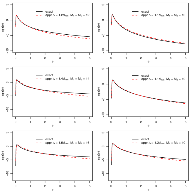
Figure S1: Exact and approximate log prior densities of $\vartheta$ for the Matérn covariance function based on the $10\times 10$ sampling design in $[0,1]^{2}$. The left panels are for models with constant mean, the right panels for models with non–constant mean, and from top to bottom $\nu=0.5,1.5$ and $2.5$.

S4. Sensitivity of the Approximate Reference Priors to the Tuning Constants

To illustrate how sensitive approximate reference priors are to the tuning constants $\Delta$ and $M_{1}$ (for simplicity $M_{2}=M_{1}$), consider the model with mean zero and Matérn correlation function with $\nu=0.5$. Figure S2 displays approximate reference priors of $\vartheta$ for different values of $\Delta$ and $M_{1}=12$ fixed (left), as well as approximate reference priors for different values of $M_{1}$ and $\Delta=0.09$ fixed (right). These show that the approximations are more sensitive to $\Delta$ than to $M_{1}$, so the tuning of the former is more important. Section 5 provides some guidelines for the selection of these tuning constants. It may also be noted that these constants could be viewed as hyperparameters and estimated using empirical Bayes.

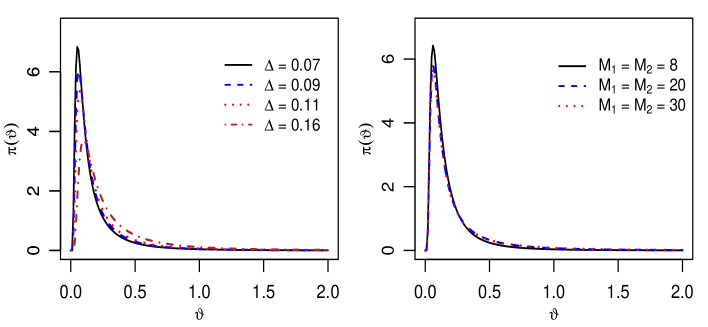
Figure S2: Sensitivity assessment of the approximate reference priors to tuning constants. Left: $M_{1}=M_{2}=12$ fixed. Right: $\Delta=0.09$ fixed.

S5. Comparison of Frequentist Properties of Bayesian Inferences Based on Several Default Priors and MLE

A useful way to evaluate default priors is through the study of frequentist properties of the resulting Bayesian inferences (Ghosh and Mukerjee, 1992). It has been found for a variety of models that reference priors yield credible intervals with satisfactory frequentist coverage and estimators with competitive mean square errors, and this has also been the case for spatial models; see Berger et al. (2001); Ren et al. (2013); Gu et al. (2018) and the references therein.

We use a simulation experiment to compare frequentist properties of Bayesian procedures based on the exact and approximate reference priors, as well as those based on a default prior suggested by Gu (2019) called “joint robust prior”. This was proposed for the (transformed) range parameters of separable correlation functions in the context of computer model emulation and calibration; for isotropic correlation functions, it reduces to an inverse gamma prior. We use $\pi^{\rm JR}(\vartheta)={\rm IG}(0.5,\sqrt{2}/100)$, where the hyperparameters were set at values recommended by Gu (2019) for the design described below. In addition, we also compare frequentist properties of purely likelihood–based inferences.

The numerical experiment is based on data in the region $\mathcal{D}=[0,1]^{2}$ simulated from Gaussian random fields with several mean and covariance functions at $n=100$ sampling locations. We consider the $10\times 10$ regular design and the irregular design displayed at the bottom left panel of Figure 6. For the mean function we use $\mu({\bf s})=1$ ($p=1$) and $\mu({\bf s})=0.15-0.65x-0.1y+0.9x^{2}-xy+1.2y^{2}$ ($p=6$), while for the correlation function we use the Matérn model (1.1) with $\sigma^{2}=1$, range parameter $\vartheta=0.2,0.4$ and $0.7$ and smoothness parameter $\nu=0.5$ and $1.5$. This setup provides a variety of scenarios in terms of trend, strength of correlation and smoothness. For each of these 12 scenarios, $3000$ data sets were simulated, and for each data set we generated $10^{4}$ posterior samples by the Monte Carlo algorithm described at the end of this part.

We compare the following frequentist properties of Bayesian procedures based on the three default priors and a purely likelihood–based procedure to make inferences about the covariance parameters:

(1) Let $[L(\boldsymbol{Z}),U(\boldsymbol{Z})]$ be either a Bayesian highest probability density credible interval or a confidence interval for a covariance parameter $\eta$. Its frequentist coverage and expected log–length are estimated from the simulated data by

$$\frac{1}{3000}\sum_{j=1}^{3000}{\bf 1}\{L(\boldsymbol{z}_{j})<\eta<U(\boldsymbol{z}_{j})\}\quad{\rm and}\quad\frac{1}{3000}\sum_{j=1}^{3000}\big{(}\log U(\boldsymbol{z}_{j})-\log L(\boldsymbol{z}_{j})\big{)},$$

respectively, where $\eta=\vartheta$ or $\sigma^{2}$, and $\boldsymbol{z}_{j}$ is the $j{\rm th}$ simulated data set. The confidence interval is obtained by evaluating the profile likelihood of $\eta$ and inverting a likelihood ratio test (Meeker and Escobar, 1995).

(2) Let $\hat{\eta}_{j}$ be either a Bayesian estimator or the MLE of $\eta$ based on $\boldsymbol{z}_{j}$. Its mean absolute error, $E\big{(}|\hat{\eta}-\eta|\big{)}$, is estimated by

$$\frac{1}{3000}\sum_{j=1}^{3000}|\hat{\eta}_{j}-\eta|.$$

For Bayesian estimation, $\hat{\eta}_{j}$ is the mode of $\pi(\eta~{}|~{}\boldsymbol{z}_{j})$ when $\eta=\vartheta$, while $\hat{\eta}_{j}$ is the median of $\pi(\eta~{}|~{}\boldsymbol{z}_{j})$ when $\eta=\sigma^{2}$.

Results for the Regular Lattice Design To compute the approximate reference prior for models with constant mean, we used $M_{1}=M_{2}=12$ and $\Delta=0.133$ when $\nu=0.5$, and $M_{1}=M_{2}=14$ and $\Delta=0.156$ when $\nu=1.5$. For models with non–constant mean, we used $M_{1}=M_{2}=10$ and $\Delta=0.122$ for both smoothness parameters. These choices were informed by the findings in Section 5.

Table S1: Frequentist coverage probability and $[$average log–length$]$ of Bayesian 95% highest probability density credible intervals of $\vartheta$ based on the three default priors, and the 95% profile likelihood confidence interval of $\vartheta$. Regular design.

			$p=1$				$p=6$
		$\vartheta=0.2$	$\vartheta=0.4$	$\vartheta=0.7$		$\vartheta=0.2$	$\vartheta=0.4$	$\vartheta=0.7$
					$\nu=0.5$
Inverse Gamma Prior		$0.963$	$0.968$	$0.976$		$0.952$	$0.980$	$0.983$
		$[2.110]$	$[3.878]$	$[4.789]$		$[5.519]$	$[5.885]$	$[6.030]$
Exact Reference Prior		$0.960$	$0.955$	$0.952$		$0.955$	$0.934$	$0.921$
		$[1.632]$	$[2.541]$	$[3.066]$		$[2.079]$	$[2.335]$	$[2.424]$
Appr Reference Prior		$0.964$	$0.955$	$0.946$		$0.958$	$0.945$	$0.935$
		$[1.535]$	$[2.008]$	$[2.313]$		$[2.181]$	$[2.388]$	$[2.459]$
MLE		$0.933$	$0.914$	$0.885$		$0.623$	$0.407$	$0.221$
		$[4.847]$	$[2.791]$	$[4.940]$		$[9.440]$	$[5.889]$	$[4.335]$
					$\nu=1.5$
Inverse Gamma Prior		$0.955$	$0.952$	$0.950$		$0.956$	$0.967$	$0.977$
		$[0.598]$	$[0.784]$	$[1.111]$		$[0.758]$	$[1.883]$	$[3.926]$
Exact Reference Prior		$0.956$	$0.953$	$0.951$		$0.959$	$0.963$	$0.957$
		$[0.596]$	$[0.781]$	$[1.106]$		$[0.742]$	$[1.227]$	$[1.857]$
Appr Reference Prior		$0.960$	$0.952$	$0.944$		$0.960$	$0.967$	$0.960$
		$[0.594]$	$[0.765]$	$[0.992]$		$[0.748]$	$[1.199]$	$[1.703]$
MLE		$0.944$	$0.930$	$0.901$		$0.772$	$0.603$	$0.395$
		$[0.684]$	$[0.714]$	$[1.021]$		$[0.755]$	$[0.837]$	$[0.798]$

Table S1 reports for different models the frequentist coverage and [average log–length] of the 95% highest probability density credible intervals (HPDCI) based on the three default priors and of the profile likelihood confidence interval (PLCI) for $\vartheta$. In almost all situations the HPDCI based on the three default priors have coverage probabilities close to the target $0.95$, with those from the approximate reference priors almost never being inferior to those from the exact reference priors. The coverage probabilities of HPDCI based on the inverse gamma prior are a bit too large in some situations. On the other hand, the coverage probabilities of PLCI tend to be smaller than the target $0.95$, and this is substantially so for models with non–constant mean. The log–lengths of the HPDCI for $\vartheta$ based on the exact and approximate reference priors are similar in most situations, with those from approximate reference priors tending to be slightly shorter than those from exact reference priors. The log–lengths of the HPDCI based on the inverse gamma prior tend to be larger, sometimes substantially so, and the same holds for PLCI.

Table S2: Frequentist coverage probability and $[$average log–length$]$ of Bayesian 95% highest probability density credible intervals of $\sigma^{2}$ based on the three default priors, and the 95% profile likelihood confidence interval of $\sigma^{2}$. Regular design.

			$p=1$				$p=6$
		$\vartheta=0.2$	$\vartheta=0.4$	$\vartheta=0.7$		$\vartheta=0.2$	$\vartheta=0.4$	$\vartheta=0.7$
					$\nu=0.5$
Inverse Gamma Prior		$0.968$	$0.973$	$0.976$		$0.960$	$0.982$	$0.984$
		$[1.577]$	$[3.565]$	$[4.541]$		$[3.723]$	$[5.061]$	$[5.395]$
Exact Reference Prior		$0.968$	$0.960$	$0.954$		$0.964$	$0.934$	$0.927$
		$[1.246]$	$[2.261]$	$[2.835]$		$[1.513]$	$[1.932]$	$[2.070]$
Appr Reference Prior		$0.971$	$0.959$	$0.943$		$0.963$	$0.945$	$0.933$
		$[1.173]$	$[1.796]$	$[2.115]$		$[1.574]$	$[1.974]$	$[2.095]$
MLE		$0.941$	$0.914$	$0.892$		$0.630$	$0.390$	$0.202$
		$[1.130]$	$[1.837]$	$[3.863]$		$[1.307]$	$[1.238]$	$[1.958]$
					$\nu=1.5$
Inverse Gamma Prior		$0.953$	$0.953$	$0.948$		$0.957$	$0.961$	$0.977$
		$[1.068]$	$[1.961]$	$[3.127]$		$[1.385]$	$[4.982]$	$[7.962]$
Exact Reference Prior		$0.954$	$0.955$	$0.945$		$0.956$	$0.958$	$0.954$
		$[1.075]$	$[1.954]$	$[3.108]$		$[1.366]$	$[3.142]$	$[5.184]$
Appr Reference Prior		$0.957$	$0.956$	$0.941$		$0.957$	$0.961$	$0.955$
		$[1.076]$	$[1.911]$	$[2.801]$		$[1.382]$	$[3.080]$	$[4.768]$
MLE		$0.940$	$0.932$	$0.908$		$0.746$	$0.577$	$0.376$
		$[1.095]$	$[1.781]$	$[2.939]$		$[1.128]$	$[1.872]$	$[2.962]$

Table S3: Mean absolute error of the posterior mode of $\vartheta$ based on the three default priors, and of the MLE of $\vartheta$ for the regular design.

			$p=1$				$p=6$
		$\vartheta=0.2$	$\vartheta=0.4$	$\vartheta=0.7$		$\vartheta=0.2$	$\vartheta=0.4$	$\vartheta=0.7$
					$\nu=0.5$
Inverse Gamma Prior		$0.046$	$0.121$	$0.287$		$0.059$	$0.162$	$0.404$
Exact Reference Prior		$0.044$	$0.120$	$0.296$		$0.055$	$0.175$	$0.440$
Appr Reference Prior		$0.043$	$0.117$	$0.294$		$0.056$	$0.169$	$0.431$
MLE		$0.064$	$0.131$	$0.412$		$0.082$	$0.195$	$0.560$
					$\nu=1.5$
Inverse Gamma Prior		$0.023$	$0.056$	$0.128$		$0.028$	$0.073$	$0.183$
Exact Reference Prior		$0.022$	$0.055$	$0.127$		$0.027$	$0.072$	$0.181$
Appr Reference Prior		$0.022$	$0.055$	$0.126$		$0.027$	$0.071$	$0.176$
MLE		$0.029$	$0.057$	$0.136$		$0.036$	$0.087$	$0.287$

Table S4: Mean absolute error of the posterior median of $\sigma^{2}$ based on the three default priors, and of the MLE of $\sigma^{2}$ for the regular design.

			$p=1$				$p=6$
		$\vartheta=0.2$	$\vartheta=0.4$	$\vartheta=0.7$		$\vartheta=0.2$	$\vartheta=0.4$	$\vartheta=0.7$
					$\nu=0.5$
Inverse Gamma Prior		$0.240$	$0.618$	$0.843$		$0.650$	$0.988$	$0.690$
Exact Reference Prior		$0.207$	$0.356$	$0.413$		$0.238$	$0.283$	$0.431$
Appr Reference Prior		$0.198$	$0.273$	$0.307$		$0.256$	$0.279$	$0.414$
MLE		$0.205$	$0.289$	$0.442$		$0.333$	$0.506$	$0.613$
					$\nu=1.5$
Inverse Gamma Prior		$0.212$	$0.389$	$0.656$		$0.287$	$1.263$	$3.013$
Exact Reference Prior		$0.213$	$0.386$	$0.645$		$0.282$	$0.639$	$0.892$
Appr Reference Prior		$0.213$	$0.373$	$0.536$		$0.287$	$0.632$	$0.863$
MLE		$0.209$	$0.348$	$0.503$		$0.287$	$0.524$	$0.720$

Table S2 reports the frequentist coverage and [average log–length] of the 95% HPDCI based on the three default priors and of the PLCI for $\sigma^{2}$. The findings are very similar to those in Table S1 for $\vartheta$. In particular, the coverage probabilities of HPDCI based on the exact and approximate reference priors are close to the target, while those of PLCI are substantially smaller than the target when the mean is non-constant. Also, the log–lengths of the HPDCI for $\sigma^{2}$ based on the inverse gamma prior tend to be the largest and those based on the approximate reference priors tend to be the smallest.

Tables S3 and S4 report the mean absolute errors (MAE) of the Bayesian estimators based on the three default priors and the MAE of the MLE. The MAE of the three Bayesian estimates of $\vartheta$ are very close to each other in all scenarios, while that of the MLE is larger. The MAE of the Bayesian estimates of $\sigma^{2}$ based on the exact and approximate reference priors are similar in most scenarios. On the other hand, the MAE of the Bayesian estimates based on the inverse gamma prior tend to be larger than the other two, sometimes substantially so, due to the tendency to overestimate $\sigma^{2}$. The same holds for the MLE, but due to the tendency to underestimate $\sigma^{2}$.

Results for the Irregular Design

To compute the approximate reference priors for models with constant mean, we used $M_{1}=M_{2}=12$ and $\Delta=0.09$ when $\nu=0.5$, and $M_{1}=M_{2}=12$ with $\Delta=0.1$ when $\nu=1.5$. For models with non–constant mean, we used $M_{1}=M_{2}=12$ and $\Delta=0.09$ for both smoothness parameters. The sampling design of this study is based on the complete random design shown in the bottom left of Figure 6.

Tables S5 and S6 report the frequentist coverage and [average log–length] of the 95% HPDCI for $\vartheta$ and $\sigma^{2}$, respectively. For most scenarios the results are about the same as those for the regular design. The coverage probabilities based on the three default priors are satisfactory as they are close to the target 0.95. They all tend to be slightly lower than nominal though, when the correlation is strong ($\vartheta=0.7$), and the coverage probabilities based on the inverse gamma prior are a bit too large in some situations. Also, similar to the findings in the regular design, the inverse gamma prior can yield substantially wider confidence intervals. Tables S7 and S8 report the MAE of the Bayesian estimators of $\vartheta$ and $\sigma^{2}$, respectively. The results are similar to the results shown in Tables S3 and S4 for the regular lattice design. Again, the MAE of $\hat{\vartheta}$ based on the three default priors are about the same, but the MAE of $\hat{\sigma}^{2}$ based on the inverse gamma prior tends to be larger than the ones based on the reference priors due to the tendency of overestimation.

Table S5: Frequentist coverage probability and $[$average log–length$]$ of Bayesian 95% highest probability density credible intervals of $\vartheta$ based on the three default priors for the irregular design.

Prior			$p=1$				$p=6$
		$\vartheta=0.2$	$\vartheta=0.4$	$\vartheta=0.7$		$\vartheta=0.2$	$\vartheta=0.4$	$\vartheta=0.7$
					$\nu=0.5$
Inverse Gamma		$0.954$	$0.968$	$0.980$		$0.969$	$0.980$	$0.971$
		$[2.316]$	$[4.076]$	$[4.853]$		$[4.995]$	$[5.613]$	$[5.872]$
Exact Reference		$0.956$	$0.947$	$0.956$		$0.957$	$0.929$	$0.899$
		$[1.777]$	$[2.672]$	$[3.155]$		$[2.133]$	$[2.362]$	$[2.427]$
Appr Reference		$0.952$	$0.935$	$0.920$		$0.957$	$0.931$	$0.911$
		$[1.524]$	$[1.999]$	$[2.282]$		$[2.167]$	$[2.385]$	$[2.461]$
					$\nu=1.5$
Inverse Gamma		$0.949$	$0.956$	$0.964$		$0.952$	$0.971$	$0.977$
		$[0.585]$	$[0.819]$	$[1.185]$		$[0.755]$	$[2.146]$	$[3.784]$
Exact Reference		$0.954$	$0.955$	$0.964$		$0.953$	$0.963$	$0.953$
		$[0.584]$	$[0.813]$	$[1.183]$		$[0.738]$	$[1.329]$	$[1.937]$
Appr Reference		$0.951$	$0.953$	$0.951$		$0.948$	$0.963$	$0.953$
		$[0.581]$	$[0.784]$	$[1.013]$		$[0.741]$	$[1.253]$	$[1.733]$

Table S6: Frequentist coverage probability and $[$average log–length$]$ of Bayesian 95% highest probability density credible intervals of $\sigma^{2}$ based on the three default priors for the irregular design.

Prior			$p=1$				$p=6$
		$\vartheta=0.2$	$\vartheta=0.4$	$\vartheta=0.7$		$\vartheta=0.2$	$\vartheta=0.4$	$\vartheta=0.7$
					$\nu=0.5$
Inverse Gamma		$0.967$	$0.967$	$0.980$		$0.973$	$0.981$	$0.990$
		$[1.946]$	$[3.804]$	$[4.634]$		$[4.074]$	$[5.165]$	$[5.482]$
Exact Reference		$0.966$	$0.957$	$0.958$		$0.960$	$0.923$	$0.907$
		$[1.454]$	$[2.329]$	$[2.949]$		$[1.683]$	$[2.017]$	$[2.118]$
Appr Reference		$0.965$	$0.940$	$0.917$		$0.963$	$0.932$	$0.921$
		$[1.230]$	$[1.869]$	$[2.106]$		$[1.718]$	$[2.038]$	$[2.130]$
					$\nu=1.5$
Inverse Gamma		$0.950$	$0.951$	$0.960$		$0.953$	$0.971$	$0.977$
		$[1.198]$	$[2.139]$	$[3.395]$		$[1.593]$	$[5.870]$	$[9.847]$
Exact Reference		$0.955$	$0.951$	$0.958$		$0.953$	$0.963$	$0.950$
		$[1.201]$	$[2.125]$	$[3.390]$		$[1.556]$	$[3.557]$	$[5.493]$
Appr Reference		$0.954$	$0.947$	$0.947$		$0.955$	$0.964$	$0.945$
		$[1.197]$	$[2.042]$	$[2.897]$		$[1.561]$	$[3.356]$	$[4.927]$

Table S7: Mean absolute error of the posterior mode of $\vartheta$ based on the three default priors for the irregular design.

Prior			$p=1$				$p=6$
		$\vartheta=0.2$	$\vartheta=0.4$	$\vartheta=0.7$		$\vartheta=0.2$	$\vartheta=0.4$	$\vartheta=0.7$
					$\nu=0.5$
Inverse Gamma		$0.048$	$0.129$	$0.301$		$0.061$	$0.173$	$0.432$
Exact Reference		$0.047$	$0.131$	$0.313$		$0.058$	$0.190$	$0.466$
Appr Reference		$0.046$	$0.129$	$0.326$		$0.060$	$0.186$	$0.460$
					$\nu=1.5$
Inverse Gamma		$0.022$	$0.059$	$0.131$		$0.028$	$0.079$	$0.195$
Exact Reference		$0.023$	$0.059$	$0.132$		$0.028$	$0.077$	$0.192$
Appr Reference		$0.022$	$0.058$	$0.130$		$0.027$	$0.076$	$0.190$

Table S8: Mean absolute error of the posterior median of $\sigma^{2}$ based on the three default priors for the irregular design.

Prior			$p=1$				$p=6$
		$\vartheta=0.2$	$\vartheta=0.4$	$\vartheta=0.7$		$\vartheta=0.2$	$\vartheta=0.4$	$\vartheta=0.7$
					$\nu=0.5$
Inverse Gamma		$0.299$	$0.680$	$0.859$		$0.824$	$0.975$	$0.614$
Exact Reference		$0.244$	$0.377$	$0.426$		$0.267$	$0.303$	$0.484$
Appr Reference		$0.218$	$0.269$	$0.337$		$0.281$	$0.298$	$0.473$
					$\nu=1.5$
Inverse Gamma		$0.240$	$0.443$	$0.717$		$0.326$	$1.403$	$3.339$
Exact Reference		$0.240$	$0.437$	$0.699$		$0.314$	$0.769$	$0.935$
Appr Reference		$0.239$	$0.415$	$0.557$		$0.317$	$0.741$	$0.892$

Algorithm to Sample from the Posterior Distribution. We describe a non–iterative Monte Carlo algorithm to draw independent samples from the exact or approximate reference posterior distribution of $(\mbox{\boldmath$\beta$},\sigma^{2},\vartheta)$, which by its nature is more efficient than alternative iterative Markov Chain Monte Carlo algorithms. It is based on factoring the posterior as

$$\pi(\mbox{\boldmath$\beta$},\sigma^{2},\vartheta~{}|~{}\boldsymbol{z})=\pi(\mbox{\boldmath$\beta$}~{}|~{}\sigma^{2},\vartheta,\boldsymbol{z})\pi(\sigma^{2}~{}|~{}\vartheta,\boldsymbol{z})\pi(\vartheta~{}|~{}\boldsymbol{z}),$$

where

$$\pi(\mbox{\boldmath$\beta$}~{}|~{}\sigma^{2},\vartheta,\boldsymbol{z}) ={\rm N}_{p}\big{(}\hat{\mbox{\boldmath$\beta$}}_{\vartheta},\sigma^{2}(\boldsymbol{X}^{\top}\boldsymbol{\Sigma}^{-1}_{\vartheta}\boldsymbol{X})^{-1}\big{)}$$

$$\pi(\sigma^{2}~{}|~{}\vartheta,\boldsymbol{z}) ={\rm IG}\left(\frac{n-p}{2},\frac{S^{2}_{\vartheta}}{2}\right)$$

$$\pi(\vartheta~{}|~{}\boldsymbol{z}) \propto\pi(\vartheta)|\boldsymbol{\Sigma}_{\vartheta}|^{-\frac{1}{2}}|\boldsymbol{X}^{\top}\boldsymbol{\Sigma}_{\vartheta}^{-1}\boldsymbol{X}|^{-\frac{1}{2}}(S^{2}_{\vartheta})^{-\frac{n-p}{2}},$$

and $\pi(\vartheta)$ is $\pi^{\rm R}(\vartheta)$, $\pi^{\rm AR}(\vartheta)$ or the inverse gamma prior; see Section (2.1) for the definition of the terms involved. So a draw from $\pi(\mbox{\boldmath$\beta$},\sigma^{2},\vartheta~{}|~{}\boldsymbol{z})$ is obtained by sampling in turn from $\pi(\vartheta~{}|~{}\boldsymbol{z})$, $\pi(\sigma^{2}~{}|~{}\vartheta,\boldsymbol{z})$ and $\pi(\mbox{\boldmath$\beta$}~{}|~{}\sigma^{2},\vartheta,\boldsymbol{z})$. The only non–standard distribution is $\pi(\vartheta~{}|~{}\boldsymbol{z})$, which is one–dimensional since the correlation function depends on a single range parameter. To sample from it, we use the generalized ratio–of–uniforms algorithm, which is efficiently implemented in the R package rust. Details can be found in Sun (2006) and Northrop (2020).

S6. Analysis of a Data Set Simulated on an Irregular Sampling Design

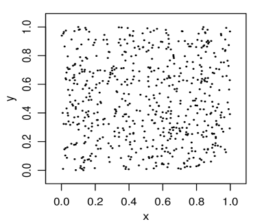
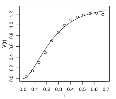
Figure S3: Left: Sampling locations of the simulated data set. Right: Integrated likelihood of $\nu$ for the simulated same data.

Here we carry out data analyses that is parallel to those done in Section 6, but based on a (simulated) data set with different features from those of the lead concentration data. Specifically, for the sampling design consisting of $n=600$ locations forming a random sample from the ${\rm unif}((0,1)^{2})$ distribution, we simulated a Gaussian random field with mean 0 and Matérn covariance function with parameters $\sigma^{2}=1$, $\vartheta=0.3$ and $\nu=1.5$. For the analysis below it is assumed that $\hat{\nu}=1.37$, obtained by maximizing the integrated likelihood of $\nu$ displayed in Figure S4 (left). Figure S3 (left) displays the sampling design, while the empirical semivariogram of the data and the semivariogram function fitted by least squares ($\hat{\sigma}^{2}=1.31$ and $\hat{\vartheta}=0.33$) are displayed in Figure S3 (right).

To compute the approximate reference prior we set $M_{1}=M_{2}=26$ and $\Delta=0.04$ (following the guidelines described in Section 5), and $\tilde{f}^{\Delta}_{\vartheta}(\mbox{\boldmath$\omega$}_{j})$ was obtained by setting $\max\{|l_{1}|,|l_{2}|\}\leq 5$. Then, two Bayesian analyses were carried out based on the exact and approximate reference priors, where samples of sizes $10^{4}$ from the corresponding posteriors of $(\beta_{1},\sigma^{2},\vartheta)$ were simulated using again the Monte Carlo algorithm described in part 5 of the Supplementary Materials.

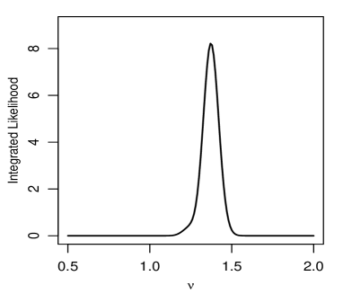
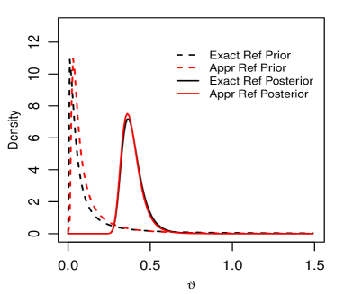
Figure S4: Left: Empirical semivariogram of the simulated data set and its least squares fit. Right: Densities of exact and approximate marginal reference priors and posteriors of $\vartheta$ for the simulated data set.

Figure S4 (right) displays the (normalized) exact and approximate reference priors of $\vartheta$, as well as their corresponding posteriors. The prior densities exhibit a slightly larger discrepancy than those for the lead concentration data, which is attributed to the sampling design being quite irregular. Nevertheless, the difference is not large, the shape of the two priors are similar, with both placing large and small probability masses in the same regions of the parameter space, and the posterior densities are very close to each other. Table S9 reports the Bayesian estimators of the model parameters and their corresponding $95\%$ highest posterior density (HPD) credible intervals based on both posteriors, showing that both inferences are, for practical purposes, equivalent.

The computation time to draw $10^{4}$ posterior samples based on the approximate reference prior was about $2240$ seconds, while the time to do the same task based on exact reference prior was $5502$ seconds. In both the exact likelihood was used so the time difference is due to prior evaluations. Since the assumed smoothness is not equal to $m+1/2$ for some non–negative integer $m$, the evaluation of the covariance function and its derivative w.r.t. $\vartheta$ involved in the computation of the exact reference prior requires $O(n^{2})$ evaluations of Bessel functions.

Table S9: Parameter estimates of the data with an irregular sampling design using exact and approximate reference priors. The estimate $\hat{\vartheta}$ is the posterior mode, $\hat{\sigma}^{2}$ is the posterior median and $\hat{\beta}_{1}$ is the posterior mean. The 95% credible intervals are the HPD.

Prior	$\hat{\beta}_{1}$	$\hat{\sigma}^{2}$	$\hat{\vartheta}$
	$(95\%~{}{\rm CI})$	$(95\%~{}{\rm CI})$	$(95\%~{}{\rm CI})$
Exact Reference	$0.589$	$1.299$	$0.365$
	$(-0.410,1.706)$	$(0.547,2.950)$	$(0.286,0.535)$
Approximate Reference	$0.582$	$1.261$	$0.361$
	$(-0.394,1.681)$	$(0.564,2.863)$	$(0.287,0.522)$

S7. Additional References

Chipman, J.S. (1964), On Least Squares with Insufficient Observations, Journal of the American Statistical Association, 59, 1078-1111.

Dahlquist, G. and Björck, Å (2008), Numerical Methods in Scientific Computing, Volume I. SIAM.

Ghosh, J.K. and Mukerjee, R. (1992), Non–Informative Priors. In: Bayesian Statistics 4, J.M. Bernardo, J.O. Berger, A.P. Dawid and A.F.M. Smith (eds.), Oxford University Press, pp 195-210.

Mohammadi, M. (2016), On the Bounds for Diagonal and Off-diagonal Elements of the Hat Matrix in the Linear Regression Model, REVSTAT - Statistical Journal, 14, 75-87.

Meeker, W.Q. and L.A. Escobar. (1995), Teaching About Approximate Confidence Regions Based on Maximum Likelihood Estimation, The American Statistician, 49, 48-53.

Northrop, P. (2020), rust: Ratio–of–Uniforms Simulation with Transformation, R package version 1.3.10, https://github.com/paulnorthrop/rust.

Sedrakyan, N. (1997), About the Applications of One Useful Inequality. Kvant Journal, 97, 42-44.

Sun, X. (2006), Bayesian Spatial Data Analysis with Application to the Missouri Ozark Forest Ecosystem Project, Ph.D. Dissertation, University of Missouri.

References

- Abramowitz and Stegun (1964) Abramowitz, M. and I. Stegun (1964). Handbook of Mathematical Functions with Formulas, Graphs, and Mathematical Tables. Dover.
- Bachoc (2014) Bachoc, F. (2014). Asymptotic analysis of the role of spatial sampling for covariance parameter estimation of Gaussian processes. Journal of Multivariate Analysis 125, 1–35.
- Berger et al. (2001) Berger, J., V. De Oliveira, and B. Sansó (2001). Objective Bayesian analysis of spatially correlated data. Journal of the American Statistical Association 96, 1361–1374.
- Bose et al. (2018) Bose, M., J. Hodges, and S. Banerjee (2018). Toward a diagnostic toolkit for linear models with Gaussian–process distributed random effects. Biometrics 74, 863–873.
- Chipman (1964) Chipman, J. (1964). On least squares with insufficient observations. Journal of the American Statistical Association 59, 1078–1111.
- De Oliveira (2007) De Oliveira, V. (2007). Bayesian analysis of spatial data with measurement error. The Canadian Journal of Statistics 35, 283–301.
- De Oliveira (2010) De Oliveira, V. (2010). Objective Bayesian Analysis for Gaussian Random Fields. In: Frontiers of Statistical Decision Making and Bayesian Analysis–In Honor of James O. Berger. M.-H. Chen, D.K. Dey, P. Muller, D. Sun and K. Ye (eds.). Springer–Verlag, 497-511.
- De Oliveira et al. (1997) De Oliveira, V., B. Kedem, and D. Short (1997). Bayesian prediction of transformed Gaussian random fields. Journal of the American Statistical Association 92, 1422–1433.
- Dietrich (1994) Dietrich, C. (1994). A note on computational issues associated with restricted maximum likelihood estimation of covariance parameters. Journal of Statistical Computation and Simulation 49, 11–20.
- Diggle et al. (2010) Diggle, P., R. Menezes, and T. Su (2010). Geostatistical inference under preferential sampling. Journal of the Royal Statistical Society, Series C 59, 191–232.
- Gelfand and Schliep (2016) Gelfand, A. and E. Schliep (2016). Spatial statistics and Gaussian processes: A beautiful marriage. Spatial Statistics 18, 86–104.
- Gower (1985) Gower, J. (1985). Properties of Euclidean and Non–Euclidean distance matrices. Linear Algebra and its Applications 67, 81–97.
- Gu (2019) Gu, M. (2019). Jointly robust prior for Gaussian stochastic process in emulation, calibration and variable selection. Bayesian Analysis 14, 857–885.
- Gu et al. (2018) Gu, M., X. Wang, and J. Berger (2018). Robust Gaussian stochastic process emulation. The Annals of Statistics 46, 3038–3066.
- Handcock and Stein (1993) Handcock, M. and M. Stein (1993). A Bayesian analysis of kriging. Technometrics 35, 403–410.
- Harville (1974) Harville, D. (1974). Bayesian inference for variance components using only error contrasts. Biometrika 61, 383–385.
- Heaton et al. (2019) Heaton, M., A. Datta, A. Finley, R. Furrer, J. Guinness, R. Guhaniyogi, F. Gerber, R. Gramacy, D. Hammerling, M. Katzfuss, F. Lindgren, D. Nychka, F. Sun, and A. Zammit-Mangion (2019). A case study competition among methods for analyzing large spatial data. Journal of Agricultural, Biological, and Environmental Statistics 24, 398–425.
- Jones and Vecchia (1993) Jones, R. and A. Vecchia (1993). Fitting continuous arma models to unequally spaced spatial data. Journal of the American Statistical Association 88, 947–954.
- Katzfuss and Guinness (2021) Katzfuss, M. and J. Guinness (2021). A general framework for Vecchia approximations of Gaussian processes. Statistical Science 36, 124–141.
- Kazianka (2013) Kazianka, H. (2013). Objective Bayesian analysis of geometrically anisotropic spatial data. Journal of Agricultural, Biological, and Environmental Statistics 18, 514–537.
- Kazianka and Pilz (2012) Kazianka, H. and J. Pilz (2012). Objective Bayesian analysis of spatial data with uncertain nugget and range parameters. The Canadian Journal of Statistics 40, 304–327.
- Kitanidis (1986) Kitanidis, P. (1986). Parameter uncertainty in estimation of spatial functions: Bayesian analysis. Water Resources Research 22, 499–507.
- Laga and Kleiber (2017) Laga, I. and W. Kleiber (2017). The modified Matérn process. Stat 6, 241–247.
- Mohammadi (2016) Mohammadi, M. (2016). On the bounds for diagonal and off-diagonal elements of the hat matrix in the linear regression model. REVSTAT - Statistical Journal 14, 75–87.
- Muré (2021) Muré, J. (2021). Propriety of the reference posterior distribution in Gaussian process modeling. The Annals of Statistics 49, 2356–2377.
- Paciorek (2007) Paciorek, C. (2007). Bayesian smoothing with Gaussian processes using Fourier basis functions in the spectralGP package. Journal of Statistical Software 19, 1–38.
- Paulo (2005) Paulo, R. (2005). Default priors for Gaussian processes. The Annals of Statistics 33, 556–582.
- Ren et al. (2012) Ren, C., D. Sun, and C. He (2012). Objective Bayesian analysis for a spatial model with nugget effects. Journal of Statistical Planning and Inference 142, 1933–1946.
- Ren et al. (2013) Ren, C., D. Sun, and S. Sahu (2013). Objective Bayesian analysis of spatial models with separable correlation functions. The Canadian Journal of Statistics 41, 488–507.
- Royle and Wikle (2005) Royle, J. A. and C. Wikle (2005). Efficient statistical mapping of avian count data. Environmental and Ecological Statistics 12, 225–243.
- Schoenberg (1937) Schoenberg, I. (1937). On certain metric spaces arising from Euclidean spaces by a change of metric and their imbedding in Hilbert space. Annals of Mathematics 38, 787–793.
- Sedrakyan (1997) Sedrakyan, N. (1997). About the applications of one useful inequality. Kvant Journal 97, 42–44.
- Stein (1999) Stein, M. (1999). Interpolation of Spatial Data: Some Theory for Kriging. Springer–Verlag.
- Varin et al. (2011) Varin, C., N. Reid, and D. Firth (2011). An overview of composite likelihood methods. Statistica Sinica 21, 5–42.
- Vecchia (1985) Vecchia, A. (1985). A general class of models for stationary two–dimensional random processes. Biometrika 72, 281–291.
- Yaglom (1987) Yaglom, A. (1987). Correlation Theory of Stationary and Related Random Functions I: Basic Results. Springer–Verlag.
- Zimmerman (2010) Zimmerman, D. (2010). Likelihood–Based Methods. In: Handbook of Spatial Statistics, A.E. Gelfand, P.J. Diggle, M. Fuentes and P. Guttorp (eds.). CRC Press, 45-56.