Uphill Roads to Variational Tightness: Monotonicity and Monte Carlo Objectives

Abstract

We revisit the theory of importance weighted variational inference (IWVI), a promising strategy for learning latent variable models. IWVI uses new variational bounds, known as Monte Carlo objectives (MCOs), obtained by replacing intractable integrals by Monte Carlo estimates—usually simply obtained via importance sampling. Burda, Grosse and Salakhutdinov (2016) showed that increasing the number of importance samples provably tightens the gap between the bound and the likelihood. Inspired by this simple monotonicity theorem, we present a series of nonasymptotic results that link properties of Monte Carlo estimates to tightness of MCOs. We challenge the rationale that smaller Monte Carlo variance leads to better bounds. We confirm theoretically the empirical findings of several recent papers by showing that, in a precise sense, negative correlation reduces the variational gap. We also generalise the original monotonicity theorem by considering non-uniform weights. We discuss several practical consequences of our theoretical results. Our work borrows many ideas and results from the theory of stochastic orders.

1 Introduction

Often, objective functions that arise in machine learning applications involve seemingly intractable high-dimensional integrals. Examples include likelihood-based inference of latent variable models (because the likelihood can be written as an integral over the latent space) or models with unnormalised densities (a.k.a. energy-based models, because they involve intractable normalising constants), hard attention problems (because they involve marginalising over all possible “glances” of the observations, see e.g. Ba et al., 2015), or information-theoretic representation learning (see e.g. Alemi et al., 2017). Variational inference constitutes a toolbox of techniques that tackle this issue by replacing the objective function to maximise by a lower bound of it (that is supposed to be easier to compute and/or optimise).

A recent and promising approach to variational inference was proposed by Burda, Grosse and Salakhutdinov (2016), notably building on prior work by Bornschein and Bengio (2015). The idea is simply to replace the intractable integrals by Monte Carlo estimates of it, and optimise the expected value of this approximation with respect to both model parameters and the randomness induced by the Monte Carlo approximation. Following Mnih and Rezende (2016), these new bounds are called Monte Carlo objectives (MCOs), and are typically obtained using importance sampling with a parametrised posterior that can be optimised. This new flavour of variational inference is usually called importance weighted variational inference (IWVI).

While they were originally developed to learn unsupervised deep latent variable models similar to variational autoencoders (VAEs, Kingma and Welling, 2014; Rezende, Mohamed and Wierstra, 2014), MCOs have been successfully applied to a diverse family of problems, including inference for Gaussian processes (Salimbeni et al., 2019), sequential models (Maddison et al., 2017; Naesseth et al., 2018; Le et al., 2018) or exponential random graphs (Tan and Friel, 2020), missing data imputation (Mattei and Frellsen, 2019; Ipsen, Mattei and Frellsen, 2021), causal inference (Josse, Mayer and Vert, 2020), neural spike inference (Speiser et al., 2017), dequantisation (Hoogeboom, Cohen and Tomczak, 2020), verification of deep discriminative models (Che et al., 2020), and general Bayesian inference (Domke and Sheldon, 2018, 2019).

These empirical successes have been calling for theoretical developments. For example, a natural question is then: how do properties of the Monte Carlo estimate translate into properties the variational bound? This question, which is the main topic of this paper, has until now mostly been tackled from an asymptotic point of view. More specifically, most results are concerned with the behaviour of MCOs when the number of Monte Carlo samples go to infinity (or when the variance goes to zero). This contrasts with the fact that, in practice, the number of samples rarely exceeds a few dozens (for computational reasons), and the variance is very large if not infinite. Motivated by this gap between theory and practice, our perspective here is non-asymptotic. One exception to the asymptotic focus is the beautifully simple result proven by Burda, Grosse and Salakhutdinov (2016): when the weights are exchangeable, increasing the number of samples always improves the tightness of the bound. This monotonicity theorem, which we will refer to as sample monotonicity, is the main inspiration of our paper.

1.1 Contributions and organisation of the paper

We begin by a review of the theory and applications of MCOs (Section 2), that we use to justify a quite general mathematical framework. Then, we explore the interplay between MC properties and variational tightness by gradually increasing the strength of the assumtions:

• We start in Section 3 by considering general estimates (not necessarily based on importance sampling). This leads us to challenge the popular heuristic that reducing MC variance improves the bound. We propose the stronger notion of convex order in order to control the tightness of the bound.

• We then consider general multiple importance sampling, with potentially different proposals (Section 4), and leverage the theory of stochastic orders to show that negative dependence provably leads to better bounds (Theorem 1), confirming theoretically several recent works.

• Adding the assumption that the weights are exchangeable, we present a generalisation of the monotonicity theorem of Burda, Grosse and Salakhutdinov (2016), that we trace back to Marshall and Proschan (1965).

Along the way, we discuss some practical consequences of our theoretical results.

2 Variational inference using Monte Carlo objectives

In this section, we present the general context of variational inference using Monte Carlo objectives. We briefly review prior work and present a general mathematical framework to analyse these objectives.

We consider some data $\mathbf{x}\in\mathcal{X}$ governed by a latent variable $\mathbf{z}\in\mathcal{Z}$ through a model with density

$$p(\mathbf{x},\mathbf{z})=p(\mathbf{z})p(\mathbf{x}|\mathbf{z}),$$ (1)

with respect to a dominating measure on $\mathcal{X}\times\mathcal{Z}$. We use densities because they are more conventionally used in the latent variable model literature, although a more general measure-theoretic framework could also be contemplated, in the fashion of Domke and Sheldon (2019, Appendix B). The model (1) may, or may not be Bayesian, depending on whether or not unknown parameters are included in the latent variable $\mathbf{z}$.

2.1 Inference via Monte Carlo objectives

Typically, the latent variable models we focus on depend on many parameters that we would like to learn via (potentially approximate) maximum likelihood. Since $\mathbf{z}$ is hidden and only $\mathbf{x}$ is observed, the log-likelihood (or log-marginal likelihood if the model is Bayesian) is equal to

$$\ell=\log p(\mathbf{x})=\log\int_{\mathcal{Z}}p(\mathbf{x|\mathbf{z}})p(\mathbf{z})d\mathbf{z}.$$ (2)

A fruitful idea to approach $\ell$ is to replace the typically intractable integral $p(\mathbf{x})$ inside the logarithm by a Monte Carlo estimate of it. Of particular interest are unbiased estimates, since they lead to lower bounds of the likelihood $\ell$. Indeed, if $R$ is a random variable such that $R>0$ and $\mathbb{E}[R]=p(\mathbf{x})$, then the quantity $\mathcal{L}=\mathbb{E}[\log R]$ is a lower bound of the likelihood $\ell$, by virtue of Jensen’s (jensen1905; 1906) inequality and the concavity of the logarithm. Moreover, the fact that, in $\mathcal{L}$, the expectation is now located outside of the logarithm means that $\mathcal{L}$ is more suited for stochastic optimisation techniques (which require unbiased estimates of the gradient of the objective function, see e.g. Bottou, Curtis and Nocedal, 2018). The lower bound $\mathcal{L}$ is called a Monte Carlo objective (MCO), and is usually maximised in lieu of the likelihood.

In this paper, we will study in particular importance sampling estimates of the form

$$R_{K}=\frac{1}{K}\sum_{k=1}^{K}\frac{p(\mathbf{x}|\mathbf{z}_{k})p(\mathbf{z}_{k})}{q(\mathbf{z}_{k}|\mathbf{x})},$$ (3)

where $\mathbf{z}_{1},\ldots,\mathbf{z}_{K}$ follow a proposal distribution $q(\mathbf{z}_{1},\ldots,\mathbf{z}_{K}|\mathbf{x})$ that usually is a function of the data $\mathbf{x}$ (e.g. via a neural network, as in VAEs). The corresponding MCO is then $\mathcal{L}_{K}=\mathbb{E}[\log R_{K}]$, which may be optimised using stochastic optimisation.

2.2 A brief history of MCOs and IWVI

Using importance sampling to approximate a (marginal) likelihood is quite an old idea (see e.g. Geweke, 1989, and references herein). The idea to use this approximation as an objective function for inference is not new either: for example Monte Carlo maximum likelihood (MCML, see e.g. Geyer, 1994, and references herein) is a popular inference technique that aims at maximising the approximation $\log R$ of the likelihood. Until now, it seems that the connections between MCML and MCOs have not been discussed in the literature. For this reason, let us spend a few lines on this. Essentially, MCML differs from the MCO approach in three ways:

• the objective function of MCML is the random quantity $\log R$, while a MCO is a deterministic function $\mathbb{E}[\log R]$,

• a MCO is generally jointly optimised over both the model parameters, i.e. the parameters of the distribution $p(\mathbf{x})$, and the parameters of the proposal distribution $q$, while MCML generally separates the two steps,

• MCOs have deep connections with variational inference, and can be interpreted as divergences between the posterior distribution of the latent variables and an approximation of it (Domke and Sheldon, 2018, 2019).

The reweighted wake-sleep (RWS) algorithm of Bornschein and Bengio (2015) is one step closer to IWVI. The idea of RWS is to repeat the following steps:

• wake-phase: the bound $\mathcal{L}$ is optimised with respect to the model parameters,

• sleep-phase: the proposal $q(\mathbf{z}|\mathbf{x})$ is optimised by minimising its Kullback-Leibler divergence to the true posterior $p(\mathbf{z}|\mathbf{x})$.

Both steps generally involve approximate optimisation by performing a few stochastic gradient steps. The main difference between RWS and IWVI is that RWS involves two objective functions to be optimised alternatively, and IWVI maximises a single objective: the MCO. Interesting discussions on the links between RWS and IWVI include Dieng and Paisley (2019), Finke and Thiery (2019), Le et al. (2020), and Kim, Hwang and Kim (2020).

An important point that we will not explore in this paper is the optimisation, of MCOs. Naive stochastic gradient descent may encounter severe problems, in particular when using many samples—this issue, and some remedies, are explored for example by Rainforth et al. (2018a), Tucker et al. (2019), and Liévin et al. (2020). Regarding more applied advances, multiple references of successful applications of MCOs are listed in the beginning of the introduction of this paper (in a wide variety of domains, including e.g. causal inference, missing data imputation, Gaussian process inference, or neural imaging).

The main question that motivates this paper is: What are the properties of the function $(K,q)\mapsto\mathcal{L}_{K}(q)$? In particular, we would like to know how changing $q$ and $K$ will affect the likelihood gap $\mathcal{G}_{K}(q)=\ell-\mathcal{L}_{K}(q)$.

Quite a large body of work has been devoted to studying the asymptotics of $\mathcal{G}_{K}(q)$, as we will detail in Section 3. Our perspective here is quite different. In the spirit of the original monotonicity result of Burda, Grosse and Salakhutdinov (2016), we wish to obtain non-asymptotic guarantees about the behaviour of $\mathcal{L}_{K}(q)$ and $\mathcal{G}_{K}(q)$ when $K$ and $q$ vary.

2.3 General setting and notations

Motivated by the questions above, we focus on the following formal context, which is slightly more general than the one described above.

We consider a potentially infinite sequence of positive random variables $\mathbf{w}=(w_{k})_{k\in\mathcal{K}}$ with common mean $\mu>0$. This sequence, called the sequence of importance weights, is indexed by $\mathcal{K}=\{1,\ldots,K_{\textup{max}}\}$, where $K_{\textup{max}}\in\mathbb{N}^{*}\cup\{\infty\}$. The joint distribution of $\mathbf{w}$ is denoted by $Q$. Note that we do not make any assumption on $Q$ yet (it may have diverse marginals, not be factored, not be absolutely continuous). For all $K\in\mathcal{K}$, the simple Monte Carlo estimate of $\mu>0$ is $R_{K}=S_{K}/K$, where $S_{K}=w_{1}+\ldots+w_{K}$. The sequence of Monte Carlo objectives $\boldsymbol{\mathcal{L}}(Q)=(\mathcal{L}_{K}(Q))_{K\in\mathcal{K}}$, is defined by

$$\mathcal{L}_{K}(Q) =\mathbb{E}_{Q}\left[\log\left(\frac{1}{K}\sum_{k=1}^{K}w_{k}\right)\right]=\mathbb{E}_{Q}\left[R_{K}\right]=\mathbb{E}_{Q}\left[\log S_{K}\right]-\log K.$$ (4)

It is possible to be slightly more general by replacing the uniform coefficients $1/K,\ldots,1/K$ by a vector $\boldsymbol{\alpha}$ in the $K$-simplex $\Delta_{K}$. This leads to

$$\mathcal{L}_{\boldsymbol{\alpha}}(Q)=\mathbb{E}_{Q}\left[\log\left(\boldsymbol{\alpha}^{T}\mathbf{w}\right)\right]=\mathbb{E}_{Q}\left[\log\left(\sum_{k=1}^{K}\alpha_{k}w_{k}\right)\right].$$ (5)

In particular $\mathcal{L}_{(1/K,\ldots,1/K)}(Q)=\mathcal{L}_{K}(Q)$. Jensen’s (jensen1905; 1906) inequality ensures that, since the logarithm is concave, $\mathcal{L}_{\boldsymbol{\alpha}}(Q)\leq\log\mu$. Note however that it is possible to have $\mathcal{L}_{\boldsymbol{\alpha}}(Q)=-\infty$ (we will show an example of this in the next section). We may also consider random coefficients $\boldsymbol{\alpha}\sim\nu$, where $\nu$ is a distribution over the simplex $\Delta_{K}$. In this context, we have $\mathcal{L}_{\boldsymbol{\alpha}}(Q)=\mathbb{E}_{Q}\left[\log\left(\boldsymbol{\alpha}^{T}\mathbf{w}\right)|\boldsymbol{\alpha}\right]$ and this leads to the bound $\mathbb{E}_{\nu}[\mathcal{L}_{\boldsymbol{\alpha}}(Q)]\leq\log\mu$.

In the context of latent variable models, $\mu=p(\mathbf{x})$; $\mathbf{w}$ is the sequence of importance weights; for all $K\in\mathcal{K}$, the distribution of $(w_{k})_{k\leq K}$ is the push-forward of the proposal $q(\mathbf{z}_{1},\ldots,\mathbf{z}_{K})$ by the mapping

$$(\mathbf{z}_{1},\ldots,\mathbf{z}_{K})\mapsto\left(\frac{p(\mathbf{x}|\mathbf{z}_{1})p(\mathbf{z}_{1})}{q(\mathbf{z}_{1})},\ldots,\frac{p(\mathbf{x}|\mathbf{z}_{K})p(\mathbf{z}_{K})}{q(\mathbf{z}_{K})}\right);$$

and $R_{K}$ is the unbiased estimate of the likelihood $p(\mathbf{x})$ defined by importance sampling, as in Equation (3). The non-uniform version $\mathcal{L}_{\boldsymbol{\alpha}}$ corresponds to using multiple importance sampling (see e.g. Elvira et al., 2019, for a general review). To stress the fact that $R_{K}$ depends on $\mathbf{x}$ and approximates $p(\mathbf{x})$, we will also note it $\hat{p}(\mathbf{x})$ instead of $R_{K}$ in sometimes (e.g. in Example 6).

We believe that this simple but general framework covers most ways of defining importance-sampling based MCOs, from the original ones of Burda, Grosse and Salakhutdinov (2016), corresponding to i.i.d. weights with uniform coefficients, to the more elaborated ones of Huang et al. (2019), where the weights are correlated and not identically distributed, and notably statistically dependent on their coefficients $\boldsymbol{\alpha}$.

2.4 Warm-up: sample monotonicity

As an illustration of the kinds of monotonicity results we wish to prove, let us start by re-stating the sample monotonicity result of Burda, Grosse and Salakhutdinov (2016), which is the main inspiration of this paper.

Theorem 1 (sample monotonicity, Burda, Grosse and Salakhutdinov, 2016).

If Q is exchangeable, then $\boldsymbol{\mathcal{L}}(Q)$ is nondecreasing, i.e. for all $K\in\{1,\ldots,K_{\textup{max}}-1\}$,

$$\mathcal{L}_{K}(Q)\leq\mathcal{L}_{K+1}(Q).$$ (6)

We remind that exchangeability means that permuting the indices of the weights does not change their distribution. More specifically, for any permutation $\sigma\in S(\mathcal{K})$, $(w_{\sigma(k)})_{k\in\mathcal{K}}$ and $(w_{k})_{k\in\mathcal{K}}$ are identically distributed.

The version of Theorem 1 that we presented here is slightly more general than the one of Burda, Grosse and Salakhutdinov (2016), who assumed that the weights are i.i.d. (which is a strictly stronger condition than exchangeability). Nonetheless, their proof also works under exchangeability. Another interesting preliminary remark about the proof of Burda, Grosse and Salakhutdinov (2016) is that their reasoning remains valid if the logarithm is replaced by any other concave function. Most of the results of our paper will share this general property.

While exchangeability is weaker than the i.i.d. assumption, it is stronger than just assuming that the weights are identically distributed (i.d.). A first natural question pertaining generalisations of sample monotonicity is therefore: is it sufficient to have i.d. weights? The answer is no, as shown by the following simple counter-example.

Example 1 (i.d. is not enough).

Let $x$, $y$ be i.i.d. positive random variables. Using the identically distributed (but non-exchangeable) weights $w_{1}=x$, $w_{2}=y$, $w_{3}=x$ leads to $\mathcal{L}_{2}(Q)\geq\mathcal{L}_{3}(Q)$.

Example 1 will turn out to a be consequence of a generalisation of sample monotonicity with non-uniform coefficients, see Equation (30).

3 Variance reduction as a heuristic towards tighter bounds

Variance reduction is often considered as the simplest way of improving Monte Carlo estimates. It sounds then natural to assume that variance reduction will lead to tighter bounds. We revisit this rationale here, and challenge it.

3.1 The variance heuristic

At its simplest level, what we call the variance heuristic may be informally formulated like this: in a MCO, if $\textup{Var}(R)$ gets smaller, then $R$ is a more accurate estimate of $\mathbb{E}[R]=\mu$, and the variational bound $\mathbb{E}[\log R]$ gets tighter. It is possible to be more formal by Taylor-expanding the logarithm of $R$ around $\mu$:

$$\log(R)=\log(\mu+(R-\mu))=\log(\mu)+\frac{R-\mu}{\mu}-\frac{(R-\mu)^{2}}{2\mu^{2}}+\textup{Rem}(R).$$ (7)

The Taylor remainder $\textup{Rem}(R)$ may be for example written using its integral form

$$\textup{Rem}(R,\mu)=-\int_{\mu}^{R}\frac{(R-t)^{2}}{2\mu^{2}t^{2}}dt.$$ (8)

Then, assuming that $\textup{Var}(R)$ is finite, computing the expectation leads to

$$\mathbb{E}[\log(R)]=\log(\mu)+\frac{\textup{Var}(R)}{2\mu^{2}}+\mathbb{E}[\textup{Rem}(R,\mu)].$$ (9)

The variance heuristic can then be seen as a consequence of the assumption that, in Equation (9), the variance term dominates the remainder. In other words, it can be seen as second order heuristic. There are good reasons to believe that this assumption is reasonable when $R$ is very concentrated around $\mu$ (e.g. when $\textup{Var}(R)$ is small). This is the rationale behind the results of Maddison et al. (2017, Proposition 1), Nowozin (2018, Proposition 1), Klys, Bettencourt and Duvenaud (2018), Domke and Sheldon (2019, Theorem 3), Huang and Courville (2019), and Dhekane (2020, Chapter 3). Similar ideas (in a setting more general than the one of MCOs) are also present in Rainforth et al. (2018b, Theorem 3). Huang et al. (2019, Section 4) also suggested to look at $\textup{Var}[\log R]$ as an asymptotic indication of tightness of the bound.

Let us see what might sometimes break in this line of reasoning. First, we have no guarantee that the variance is actually finite. It is even quite common to encounter infinite variance importance sampling estimates, and we will give empirical evidence that the ones commonly used in VAEs have indeed infinite variance. Even assuming that the variance is finite, there are many situations where we could expect the Taylor remainder to be non-negligible. Indeed, the radius of convergence of the logarithm as a power series is quite small (the radius of $x\mapsto\log(x)$ is $\mu$ around $\mu$). This means that even a high order heuristic will not be accurate if $R$ gets far away from its mean $\mu$.

3.2 Simple successes, simple failures

Sample monotonicity can be seen a first example of success of the variance heuristic: adding more importance weights will both reduce Monte Carlo variance and tighten the bound.

Example 2 (sample monotonicity and variance reduction).

Let $R_{K}$ be the importance sampling estimate. Let us assume that the weights are exchangeable and have finite variance. Sample monotonicity ensures that the MCO will increase. However, adding samples will also have a variance reduction effect: for all $K\in\{1,...,K_{\textup{max}}-1\}$,

$$\textup{Var}(R_{K+1})\leq\textup{Var}(R_{K}).$$ (10)

In the case of i.i.d. weights, this simply follows from $\textup{Var}(R_{K})=\textup{Var}(w_{1})/K^{2}$. In the exchangeable case, this can be shown directly or seen as a consequence of a generalised version of sample monotonicity (Theorem 3). We will see that, in fact, these two simultaneous monotonicity properties (of the bound and of the variance) are different sides of the same coin.

Let us now look at the general case where $R$ can be any unbiased Monte Carlo estimate (not necessarily obtained via importance sampling). Of course, this is an overly general setting, and some assumptions must be made in order to be able to prove something. For example, we may wonder what happens when $R$ beyond to simple families of distributions. Sometimes, things will go as foretold by the heuristic, as seen below.

Example 3 (a few successes of the variance heuristic).

Let $R$ and $R^{\prime}$ be either two gamma, two inverse gamma, or two log-normal distributions with finite and equal means and finite variances. Then

$$\textup{Var}[R]<\textup{Var}[R^{\prime}]\iff\textup{Var}[\log R]<\textup{Var}[\log R^{\prime}]\iff\mathbb{E}[\log R]>\mathbb{E}[\log R^{\prime}].$$ (11)

The proof is available in Appendix A. The fact that these are exponential families suggests that a more general result may be hidden behind Proposition 3. While interesting in its own right, such a result would not be particularly relevant in the context of MCOs. Indeed, in general, with MCOs, $R$ follows a complex distribution very unlikely to belong to an exponential family.

What does it take to violate the heuristic using these kinds of simple distributions? While comparing two inverse gammas or two log-normals always respects it, simply blending these two family is enough to get severe violations.

Example 4 (severe failure of the variance heuristic).

Let $R$ be an inverse-gamma variable with finite mean. It is possible to find a log-normal random variable $R^{\prime}$ such that

• $\mathbb{E}[R]=\mathbb{E}[R^{\prime}]$, $\textup{Var}[R]=\infty$, $\textup{Var}[R^{\prime}]<\infty$,

• $\mathbb{E}[\log R]>\mathbb{E}[\log R^{\prime}]$.

Again, the proof is available in Appendix A. In particular, we show that the gap $\mathbb{E}[\log R]-\mathbb{E}[\log R^{\prime}]$ can be made arbitrarily large by choosing the log-normal parameters (im)properly. This means that, when comparing MCOs, it is possible to be in a situation where infinitely worse variance leads to an arbitrarily better bound. It is also possible to be in a situation that is somehow the opposite of Example 4: the variance is finite, but the bound is not.

Example 5 (finite variance, infinitely loose bound).

It is possible to find random variables such that $\mathbb{E}[R]=\mu$, $\mathbb{E}[\log R]=-\infty$, and $\textup{Var}(R)<+\infty$. This is for example the case of the finite moment log-stable distributions of Carr and Wu (2003). This family is constituted of some exponentiated Lévy stable distributions (for more details, see also Robinson, 2015).

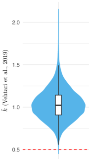
Figure 1: Importance sampling diagnostics for a VAE on MNIST. To each training digit corresponds a value of $\hat{k}$. Values of $\hat{k}$ above the dashed line correspond to digits whose weights have potentially infinite variance.

While it is not very surprising to find counter examples of these sorts, it is interesting to see that such severe failures may be observed using quite simple distributions. This phenomenon is reminiscent of the line of thought of Chatterjee and Diaconis (2018), who argued that the variance is not a very good metric for devising good importance sampling estimates.

3.3 Is the variance finite in practice?

It is often the case that importance weights have infinite variance. We provide empirical evidence that this is the case in the simple case of a VAE trained on MNIST (Figure 1). After training, we compute $10{,}000$ weights for each digits that we use to compute the $\hat{k}$ diagnostic of Vehtari et al. (2019). Most digits have a $\hat{k}>0.5$, and are therefore suspect of having infinite variance. This illustrates again the shortcomings of the variance. More details on this experiment are provided in Appendix B.

3.4 Beyond variance reduction: the convex order

While a powerful heuristic, variance reduction is not a strong enough dispersion measure to guarantee the tightening of a bound. Such a measure is provided by a branch of the theory of stochastic orders (extensively reviewed in the monograph of Shaked and Shanthikumar, 2007). The essential idea is to define binary relations $\preceq$ between distributions (or equivalently random variables) such that $R\preceq R^{\prime}$ means that, in some sense, $R$ is more concentrated that $R^{\prime}$. A popular dispersion order is the convex order (reviewed for example by Shaked and Shanthikumar, 2007, Section 3.A).

Definition 1.

Let $R\sim\pi_{1}$ and $R^{\prime}\sim\pi_{2}$ be two univariate random variables. We say that $R$ is smaller than $R^{\prime}$ in the convex order if

$$\mathbb{E}_{\pi_{1}}[\phi(R)]\leq\mathbb{E}_{\pi_{2}}[\phi(R^{\prime})],$$ (12)

for all convex functions $\phi$ such that the involved expectations exist. We denote $R\preceq_{\textup{CX}}R^{\prime}$ or $\pi_{1}\preceq_{\textup{CX}}\pi_{2}$.

Contrarily to variance reduction, which does not provide general tightening guarantees, convex ordering implies both variance reduction and bound tightening.

Proposition 1.

Let $R,R^{\prime}$ be two univariate random variables. We have

$$R\preceq_{\textup{CX}}R^{\prime}\implies\left\{\begin{matrix}\mathbb{E}[\log(R)]\geq\mathbb{E}[\log(R^{\prime})]\\ \textup{Var}(R)\leq\textup{Var}(R^{\prime})\\ \mathbb{E}[R]=\mathbb{E}[R^{\prime}]\end{matrix}\right..$$ (13)

Proof.

These are direct consequences of the concavity of the logarithm, and the convexity of $x\mapsto x^{2}$, $x\mapsto x$, and $x\mapsto-x$. ∎

This simple result means that the more concentrated the Monte Carlo estimate (in the sense of the convex order), the tighter the bound and the smaller the variance. We will see in the next sections that two successful ways of provably getting tighter bounds can be explained from the perspective of the convex order: using more importance weights, and increasing their negative dependence. In these cases, variance reduction will be merely seen as a side effect of convex domination.

Is the convex order too strong?

The fact that the inequality (12) needs to hold for every convex function $\phi$ appears like quite a strong condition. Indeed, it would be sufficient to have this for any class of functions containing $-\log$ to be able to control the tightness of the bound. For example, one might only consider decreasing convex functions. This would lead to considering monotonic convex orders, other dispersion orders which are less popular than the convex order, but has some useful properties (see e.g. Shaked and Shanthikumar, 2007, Chapter 4). In the specific case of MCOs, convex order and increasing convex order are the same. Indeed, one can show (Shaked and Shanthikumar, 2007, Theorem 4.A.35) that, if $\mathbb{E}[R]=\mathbb{E}[R^{\prime}]$, then

$$R\preceq_{\textup{CX}}R^{\prime}\iff\mathbb{E}[\phi(R)]\leq\mathbb{E}[\phi(R^{\prime})]\textup{ for all decreasing convex $\phi$}\\ \textup{such that both expectations exist}.$$ (14)

This means that the convex order is weaker than it looks. Of course, it is still stronger than just looking at the variance. Beyond a more mathematically convenient framework, what would we gain from this larger generality? The next example provides a simple illustration in the context of latent variable models.

Example 6 (Divergence control).

Let us go back to the context of latent variable models. Here, the unbiased estimate $R$, seen as a function of $\mathbf{x}$, may be viewed as an approximation of the true density of the model $p(\mathbf{x})$. To highlight this, we will denote $R=\hat{p}(\mathbf{x})$. Now how far is $\hat{p}$ from $p$? A natural way of quantifying this is to use probability divergences, for exemple $f$-divergences. For some fixed smooth convex function $f$ such that $f(1)=0$, the $f$-divergence between the density $p_{1}$ of a finite measure and a probability density $p_{2}$ is defined as

$$D_{f}(p_{1}||p_{2})=\int_{\mathcal{X}}f\left(\frac{p_{1}(\mathbf{x})}{p_{2}(\mathbf{x})}\right)p_{2}(\mathbf{x})d\mathbf{x}+f^{\prime}(1)\left(\int_{\mathcal{X}}p_{1}(\mathbf{x})d\mathbf{x}-1\right).$$ (15)

Particular cases of $f$-divergences include e.g. the popular Kullback Leibler (KL) divergence and its “reverse” version or the squared Hellinger distance, depending on the choice of $f$. In this version of the definition of $f$-divergences (seen, e.g., in Stummer and Vajda, 2010), the first density $p_{1}$ does not have to sum to one, which is fortunate because $\hat{p}$ typically will not. Indeed, the only thing we can guarantee is that $\hat{p}$ sums on average to one:

$$\mathbb{E}\left[\int_{\mathcal{X}}\hat{p}(\mathbf{x})d\mathbf{x}\right]=\int_{\mathcal{X}}\mathbb{E}\left[\hat{p}(\mathbf{x})\right]d\mathbf{x}=\int_{\mathcal{X}}p(\mathbf{x})d\mathbf{x}=1.$$ (16)

This implies that $\hat{p}$ almost surely corresponds to a finite measure. Therefore, the quantity $D_{f}(\hat{p}||p)$, which is random because $\hat{p}$ is random, is almost surely well-defined. Its average value will then be

$$\mathbb{E}[D_{f}(\hat{p}||p)] =\mathbb{E}\left[\int_{\mathcal{X}}f\left(\frac{\hat{p}(\mathbf{x})}{p(\mathbf{x})}\right)p(\mathbf{x})d\mathbf{x}\right]+f^{\prime}(1)\left(\mathbb{E}\left[\int_{\mathcal{X}}\hat{p}(\mathbf{x})d\mathbf{x}\right]-1\right)$$ (17)

$$=\int_{\mathcal{X}}\mathbb{E}\left[f\left(\frac{\hat{p}(\mathbf{x})}{p(\mathbf{x})}\right)\right]p(\mathbf{x})d\mathbf{x}.$$ (18)

Finally, using the convexity of $f$, we can conclude that

$$\left\{\forall\mathbf{x}\in\mathcal{X},\;\hat{p}_{1}(\mathbf{x})\preceq_{\textup{CX}}\hat{p}_{2}(\mathbf{x})\right\}\implies\mathbb{E}[D_{f}(\hat{p}_{1}||p)]\leq\mathbb{E}[D_{f}(\hat{p}_{2}||p)],$$ (19)

which means that the approximation of the distribution becomes better and better when the MC approximation gets more concentrated.

This example shows that convex domination can be useful in the LVM context beyond controlling bound tightness. We will use (19) later in the paper to show some monotonicty properties of $f$-divergences in the specific case of importance sampling estimates.

4 Negative dependence and tighter bounds

A popular branch of variance reduction techniques is based on negative dependence. In its simplest form, this idea is based on the fact that

$$\textup{Var}(\boldsymbol{\alpha}^{T}\mathbf{w})=\sum_{k=1}^{K}\alpha_{k}^{2}\textup{Var}(w_{k})+2\sum_{1\leq k<k^{\prime}\leq K}\alpha_{k}\alpha_{k^{\prime}}\textup{Cov}(w_{k},w_{k^{\prime}}),$$ (20)

which means that negative covariances in the right hand side of Equation (20) will lead to a smaller variance of $\boldsymbol{\alpha}^{T}\mathbf{w}$. Anthitetic sampling is for example a famous variance reduction technique based on this idea (see e.g. Owen, 2013, Section 8.2). A more refined approach is to leverage determinantal point processes (Bardenet and Hardy, 2020).

Variants of this rationale were used successfully in the MCO context by Klys, Bettencourt and Duvenaud (2018), Huang et al. (2019), Ren, Zhao and Ermon (2019), Wu, Goodman and Ermon (2019), and Domke and Sheldon (2019). Their motivations were essentially based on variants of the variance heuristic: since negative dependence can reduce the variance, it might also improve the bound. Our goal here is to prove that negative dependence can indeed tighten the bound, giving hereby a non-asymptotic theoretical justification for the works aforementioned.

4.1 Comparing dependence with the supermodular order

Let $\mathbf{w}\sim Q_{1}$ and $\mathbf{v}\sim Q_{2}$ be two $K$-dimensional random variables with identical marginals, i.e. $w_{k}\overset{d}{=}v_{k}$ for all $k\in\{1,...,K\}$ (some would say that $Q_{1}$ and $Q_{2}$ belong to the same Fréchet class, see e.g. ). What mathematical sense could we give to the sentence “the coordinates of $\mathbf{w}$ are more negatively dependent than those of $\mathbf{v}$”? Again, stochastic orders provide good tools for assessing this. Indeed, the idea of dependence orders is to define binary relations $\preceq$ between distributions such that $Q_{1}\preceq Q_{2}$ means that, in some sense, the coordinates of $\mathbf{w}\sim Q_{1}$ are more negatively dependent that those of $\mathbf{v}\sim Q_{2}$. We will review in this section a few of these dependence-based stochastic orders (a more detailed overview may be found in Shaked and Shanthikumar, 2007, Chapter 9, or Rüschendorf, 2013, Chapter 6). We focus on the supermodular order, which, as we will see in the next subsection, is the most closely related to Monte Carlo objectives. We first need to define supermodular functions.

Definition 2.

A function $\phi:\mathbb{R}^{K}\rightarrow\mathbb{R}$ is supermodular if, for all $\mathbf{x},\mathbf{y}\in\mathbb{R}^{K}$,

$$\phi(\min(\mathbf{x},\mathbf{y}))+\phi(\max(\mathbf{x},\mathbf{y}))\geq\phi(\mathbf{x})+\phi(\mathbf{y}).$$ (21)

In Equation 21, the min and max functions are applied elementwise. We can now define the supermodular order.

Definition 3.

Let $Q_{1}$ and $Q_{2}$ be two probability distributions over $\mathbb{R}^{K}$. We say that $Q_{1}$ is smaller than $Q_{2}$ in the supermodular order when

$$\mathbb{E}_{Q_{1}}[\phi(\mathbf{w})]\leq\mathbb{E}_{Q_{2}}[\phi(\mathbf{v})]$$

for all supermodular functions $\phi$ such that the involved expectations exist. We denote $Q_{1}\preceq_{\textup{SM}}Q_{2}$.

As a first remark, note that $Q_{1}\preceq_{\textup{SM}}Q_{2}$ implies that $Q_{1}$ and $Q_{2}$ have identical marginals.

The supermodular order is one of the most popular stochastic orders when it comes to quantify dependence (see e.g. Müller and Scarsini, 2000; Shaked and Shanthikumar, 2007, Chapter 9), notably in the economics and insurance literature (see e.g. Müller, 1997; Meyer and Strulovici, 2012; Meyer and Strulovici, 2015). Joe (1997, Section 2.2.3) proposed a set of nine axioms that would characterise good dependence orders. A few years later, Müller and Scarsini (2000) proved that the supermodular order satisfied all of these desirable properties.

Here is a simple example of supermodular ordering: for two distributions $Q_{1},Q_{2}$ with identical marginals, if the coordinates of $\mathbf{w}\sim Q_{1}$ are negatively associated, and those of $\mathbf{v}\sim Q_{2}$ are independent, then $Q_{1}\preceq_{\textup{SM}}Q_{2}$ (Christofides and Vaggelatou, 2004).

4.2 The more negatively dependent the weights, the tighter the bound

An important example of supermodular function is the following: let $\phi$ be a convex function and $\boldsymbol{\alpha}$ a vector with non-negative coefficients, then $\mathbf{w}\mapsto\phi\left(\boldsymbol{\alpha}^{T}\mathbf{w}\right)$ is supermodular. Using this fact with $\phi=-\log$ immediately immediately leads to

$$\mathbf{w}\preceq_{\textup{SM}}\mathbf{v}\implies\boldsymbol{\alpha}^{T}\mathbf{w}\preceq_{\textup{CX}}\boldsymbol{\alpha}^{T}\mathbf{v},$$ (22)

and to the following monotonicity theorem.

Theorem 2 (negative dependence tightens the bound).

For all pairs $Q_{1},Q_{2}$ of probability distributions over $\mathbb{R}^{K}$,

$$Q_{1}\preceq_{\textup{SM}}Q_{2}\implies\mathcal{L}_{\boldsymbol{\alpha}}(Q_{1})\geq\mathcal{L}_{\boldsymbol{\alpha}}(Q_{2}).$$ (23)

In other words, the lower bound gets tighter when the weights get more negatively dependent (in the supermodular sense). This gives a theoretical support to the successful recent applications of negative dependence to tighten variational bounds. Beyond bound tightening, combining Equation (22) and Example 6 ensures that more negative dependence will also provide more accurate likelihood estimators according to any $f$-divergence.

The main limitation of our result is that it is difficult to control the supermodular order in practice. A silver lining to this is the central role played by the supermodular order among dependence measures. In particular, the popular notion of negative association is in a sense stronger than the supermodular order (for a more general result than the simple one from Christofides and Vaggelatou, 2004, cited above, see Shaked and Shanthikumar, 2007, Theorem 9.E.8). For instance, when $K=2$,

$$\textup{Cov}_{Q_{1}}(h_{1}(w_{1}),h_{2}(w_{2}))\leq\textup{Cov}_{Q_{2}}(h_{1}(v_{1}),h_{2}(v_{2}))$$ (24)

for all increasing functions $h_{1}$ and $h_{2}$ implies that $Q_{1}\preceq_{\textup{SM}}Q_{2}$.

5 A non-uniform generalisation of Burda’s result via majorisation

In this section, we wish to extend sample monotonicty to the case of non-uniform bounds $\mathcal{L}_{\boldsymbol{\alpha}}(Q)$. To this end, we use the concept of majorisation that was popularised in the influential book of Hardy, Littlewood and Pólya (1952, Chapter 2). For a good review of majorisation and its applications, see Marshall, Olkin and Arnold (2011).

Definition 4 (majorisation).

Let $\boldsymbol{\alpha},\boldsymbol{\beta}\in\Delta_{K}$. We say that $\boldsymbol{\alpha}$ majorises $\boldsymbol{\beta}$ if $\boldsymbol{\beta}$ is in the convex hull of all vectors obtained by permuting the coordinates of $\boldsymbol{\alpha}$. We denote $\boldsymbol{\alpha}\preceq_{\textup{M}}\boldsymbol{\beta}$. This is equivalent to the condition

$$\forall k\in\{1,...,K\},\;\sum_{j=1}^{k}\alpha^{(j)}\leq\sum_{j=1}^{k}\beta^{(j)},$$ (25)

where $({\alpha}^{(1)},...,{\alpha}^{(K)})$ and $({\beta}^{(1)},...,{\beta}^{(K)})$ are reordered versions of $\boldsymbol{\alpha}$ and $\boldsymbol{\beta}$, sorted in decreasing order.

Roughly speaking, $\boldsymbol{\alpha}\preceq_{\textup{M}}\boldsymbol{\beta}$ when the coefficients of $\boldsymbol{\beta}$ are “more spread out” than those of $\boldsymbol{\alpha}$. Indeed, for example, we have for all $\boldsymbol{\alpha}\in\Delta_{K}$,

$$(1/K,...,1/K)\preceq_{\textup{M}}\boldsymbol{\alpha}\preceq_{\textup{M}}(1,0,...,0).$$ (26)

Other examples of majorisation can be found in Marshall, Olkin and Arnold (2011), notably in Chapters 1 and 5.

We can now state and prove the more general version of sample monotonicity of Marshall and Proschan (1965). Note that our proof is quite different, but not particularly original. Our proof is similar in spirit to a simple proof of the result that any convex and symmetric function is Schur-convex, i.e. respects the majorisation order (see e.g. the proof of Marshall, Olkin and Arnold, 2011, Proposition C.3).

Theorem 3 (Marshall and Proschan, 1965).

Let $\boldsymbol{\alpha},\boldsymbol{\beta}\in\Delta_{K}$. If the weights are exchangeable, then

$$\boldsymbol{\alpha}\preceq_{\textup{M}}\boldsymbol{\beta}\implies\boldsymbol{\alpha}^{T}\mathbf{w}\preceq_{\textup{CX}}\boldsymbol{\beta}^{T}\mathbf{w}.$$ (27)

Proof.

Let $\phi$ be a convex function. Exchangeabity of the weights and convexity of $\phi$ imply that the function $f:\boldsymbol{x}\mapsto\mathbb{E}_{Q}[\phi(\boldsymbol{x}^{T}\mathbf{w})]$ is convex and symmetric (i.e. permutation-invariant). Consider now $\boldsymbol{\alpha}\preceq_{\textup{M}}\boldsymbol{\beta}$. Then, $\boldsymbol{\alpha}$ belongs to the convex hull of all vectors obtained by permuting the coordinates of $\boldsymbol{\alpha}$. Since $f$ is symmetric, all these permuted vectors lead to the same value of $f$. Convexity of $f$ then leads to $\mathbb{E}_{Q}[\phi(\boldsymbol{\alpha}^{T}\mathbf{w})]\leq\mathbb{E}_{Q}[\phi(\boldsymbol{\beta}^{T}\mathbf{w})]$. ∎

This immediately gives a non-uniform version of sample monotonicity, that can be interpreted this way: the more spread out the coefficients $\alpha_{1},...,{\alpha}_{K}$ of the weights, the tighter the bound.

Corollary 1 (non-uniform sample monotonicity).

Let $\boldsymbol{\alpha},\boldsymbol{\beta}\in\Delta_{K}$. If the weights are exchangeable, then

$$\boldsymbol{\alpha}\preceq_{\textup{M}}\boldsymbol{\beta}\implies\mathcal{L}_{\boldsymbol{\alpha}}(Q)\geq\mathcal{L}_{\boldsymbol{\beta}}(Q).$$ (28)

There are several immediate corollaries of Corollary 1. The first one is the original sample monotonicity result of Burda, Grosse and Salakhutdinov (2016), stated as Theorem 1 in our paper . Indeed, this result is direct consequence of the fact that $(1/(K+1),...,1/(K+1))\preceq_{\textup{M}}(1/K,...,1/K,0)$. More generally, the left hand of Equation (26) implies that, when the importance weights are exchangeable,

$$\mathcal{L}_{\boldsymbol{\alpha}}(Q)\leq\mathcal{L}_{K}(Q),$$ (29)

which means that if the weights are exchangeable, it is optimal to use the standard uniform average. The practical guideline that comes with this is that we should not bother learning non-uniform coefficients when the weights are exchangeable. This is quite in line with the reasoning of Huang et al. (2019), who advocated the use of non-uniform coefficients together with non-exchangeable importance weights.

Less importantly, another corollary is Example 1. Indeed, using under the setup of Example 1, the fact that $(1/2,1/2)\preceq_{\textup{M}}(2/3,1/3)$ implies that

$$\mathcal{L}_{2}(Q)=\mathbb{E}\left[\frac{x+y}{2}\right]\geq\mathbb{E}\left[\frac{2x}{3}+\frac{y}{3}\right]=\mathbb{E}\left[\frac{x+y+x}{3}\right]=\mathcal{L}_{3}(Q).$$ (30)

Another consequence of Theorem 3 and Example 6 is that the $f$-divergence between the likelihood and its importance-sampling approximation is a decreasing function of $K$.

6 Conclusion

We have presented several simple results inspired by the sample monotonicity theorem of Burda, Grosse and Salakhutdinov (2016). Further refinements and generalisations appear possible. For instance, in the non-exchangeable case, it seems reasonable that using non-uniform coefficients can be optimal, but our paper does not offer a theory for this.

Another important question concerns additional applications of such results. Concerning negative dependence, an interesting question is whether or not these sorts of investigations could provide a guide to design proposal distributions with the “right amount of correlation” required to tighten bounds.

As a concluding note, let us mention that we were surprised to notice that stochastic orders have been seldom applied to studying Monte Carlo methods. Among the few papers that we found that explored this connection, a nice line of work originated by Andrieu and Vihola (2016) has used the convex order to analyse Markov chain Monte Carlo algorithms (Bornn et al., 2017; Leskelä and Vihola, 2017; Andrieu, Lee and Vihola, 2018). Other interesting work using stochastic order in a Monte Carlo setting include Goldstein, Rinott and Scarsini (2011, 2012) and Bernard and Leduc (2019). We believe that the convex order provides a quite compelling way of assessing the accuracy of different Monte Carlo approximations, and can be a very valuable tool within the Monte Carlo theoretical toolbox.

[Acknowledgments]

This work has been supported by the French government, through the 3IA Côte d’Azur Investments in the Future project managed by the National Research Agency (ANR) with the reference number ANR-19-P3IA-0002. Furthermore, it was supported by the Novo Nordisk Foundation (NNF20OC0062606 and NNF20OC0065611) and the Independent Research Fund Denmark (9131-00082B).

Appendix A. Proofs of examples

Example 3

Let $R$ and $R^{\prime}$ be either two gamma, two inverse gamma, or two log-normal distributions with finite and equal means and finite variances. Then

$$\textup{Var}(R)<\textup{Var}[R^{\prime}]\iff\textup{Var}(\log R)<\textup{Var}[\log R^{\prime}]\iff\mathbb{E}[\log R]>\mathbb{E}[\log R^{\prime}].$$ (31)

Proof.

We will treat each family separately.

The gamma case.

Let $R\sim\mathcal{G}(\alpha,\beta)$ and $R^{\prime}\sim\mathcal{G}(a,b)$ with $\alpha,\beta,a,b>0$. We remind that

$$\mathbb{E}[R]=\frac{\alpha}{\beta},\;\mathbb{E}[\log R]=\psi(\alpha)-\log(\beta),\;\textup{Var}(\log R)=\psi^{(1)}(\alpha),\;\text{Var}(R)=\frac{\alpha}{\beta^{2}},$$ (32)

where $\psi$ is the digamma function and $\psi^{(1)}$ is the trigamma function. Assuming that $R$ and $R^{\prime}$ have the same mean leads to $a=\alpha b/\beta$. We have then:

$$\textup{Var}(R)<\textup{Var}[R^{\prime}]\iff\frac{\alpha}{\beta^{2}}<\frac{a}{b^{2}}=\frac{\alpha}{\beta b}\iff\beta>b,$$ (33)

and, using the fact that $\psi^{(1)}$ decreases,

$$\textup{Var}(\log R)<\textup{Var}[\log R^{\prime}]\iff\psi^{(1)}(\alpha)<\psi^{(1)}(a)\iff\alpha>a\iff\beta>b.$$ (34)

Regarding the bounds, we have

$$\mathbb{E}[\log R]-\mathbb{E}[\log R^{\prime}] =\psi(\alpha)-\psi\left(\frac{\alpha b}{\beta}\right)+\log\left(\frac{b}{\beta}\right)$$ (35)

$$=\psi(\alpha)-\log(\alpha)-\left(\psi\left(\frac{\alpha b}{\beta}\right)-\log\left(\frac{\alpha b}{\beta}\right)\right).$$ (36)

Therefore, since the function $\psi-\log$ is increasing (see e.g. Alzer, 1997, Theorem 1), we get

$$\mathbb{E}[\log R]>\mathbb{E}[\log R^{\prime}]\iff\alpha>\frac{\alpha b}{\beta}\iff\beta>b.$$ (37)

The inverse gamma case.

Let $R\sim\mathcal{IG}(\alpha,\beta)$ and $R^{\prime}\sim\mathcal{IG}(a,b)$ with $\alpha,\beta,a,b>0$. Since we assume that $R$ and $R^{\prime}$ have finite variance, we must have $\alpha,a>2$. We remind that

$$\mathbb{E}[R]=\frac{\beta}{\alpha-1},\;\mathbb{E}[\log R]=\log(\beta)-\psi(\alpha),\;\textup{Var}(\log R)=\psi^{(1)}(\alpha),\;\text{Var}(R)=\frac{\beta}{(\alpha-1)^{2}}.$$ (38)

Assuming equality of the means leads to $b=\beta(a-1)/(\alpha-1)$. We have then:

$$\textup{Var}(R)<\textup{Var}[R^{\prime}]\iff\alpha>a.$$ (39)

Since the trigamma function decreases, we also have

$$\textup{Var}(\log R)<\textup{Var}[\log R^{\prime}]\iff\alpha>a.$$ (40)

Let us now look at the bounds. We have

$$\mathbb{E}[\log R]-\mathbb{E}[\log R^{\prime}] =\psi(a)-\psi(\alpha)+\log\left(\frac{\alpha-1}{a-1}\right)$$ (41)

$$=\psi(a)-\log(a)-\left(\psi(\alpha)-\log(\alpha)\right)+\log\left(\frac{\alpha-1}{\alpha}\right)-\log\left(\frac{a-1}{a}\right).$$ (42)

Since the functions $\psi-\log$ and $x\mapsto\log((x-1)/x)$ are increasing, we get

$$\mathbb{E}[\log R]>\mathbb{E}[\log R^{\prime}]\iff\alpha>a.$$ (43)

The lognormal case.

Let $R\sim\text{log}\,\mathcal{N}(\mu,\sigma)$ and $R^{\prime}\sim\text{log}\,\mathcal{N}(m,s)$ with $\mu,m\in\mathbb{R}$ and $\sigma,s>0$. We remind that

$$\mathbb{E}[R]=e^{\mu+\sigma^{2}/2},\;\mathbb{E}[\log R]=\mu,\;\textup{Var}(\log R)=\sigma^{2},\;\text{Var}(R)=\left(e^{\sigma^{2}}-1\right)e^{2\mu+\sigma^{2}}.$$ (44)

The equality of the means implies that $2\mu+\sigma^{2}=2m+s^{2}$. Therefore, we have

$$\textup{Var}(R)<\textup{Var}[R^{\prime}] \iff\sigma^{2}<s^{2}\iff\textup{Var}(\log R)<\textup{Var}(\log R^{\prime})$$ (45)

$$\iff\sigma^{2}<2\mu+\sigma^{2}-2m$$ (46)

$$\iff m<\mu\iff\mathbb{E}[\log R^{\prime}]<\mathbb{E}[\log R].$$ (47)

∎

Example 4

Let $R$ be an inverse-gamma variable with finite mean. It is possible to find a log-normal random variable $R^{\prime}$ such that

• $\mathbb{E}[R]=\mathbb{E}[R^{\prime}]$, $\textup{Var}(R)=\infty$, $\textup{Var}[R^{\prime}]<\infty$,

• $\mathbb{E}[\log R]>\mathbb{E}[\log R^{\prime}]$.

Proof.

Let $R\sim\mathcal{IG}(\alpha,\beta)$ and $R^{\prime}\sim\text{log}\,\mathcal{N}(\mu,\sigma)$ with $\alpha\in(1,2)$, $\beta,\sigma>0$ and $\mu\in\mathbb{R}$. Since we chose $\alpha\in(1,2)$, the mean of $R$ will be finite but its variance will be infinite. To get equality of the means of $R$ and $R^{\prime}$, we further assume that

$$\mu=\log(\beta)-\log(\alpha-1)-\frac{\sigma^{2}}{2}.$$ (48)

The difference between the bounds is then equal to

$$\mathbb{E}[\log R]-\mathbb{E}[\log R^{\prime}]=-\psi(\alpha)+\log(\beta)-\mu=-\psi(\alpha)+\log(\beta)+\frac{\sigma^{2}}{2},$$ (49)

which can be arbitrarily large provided that $\sigma$ is large enough. ∎

Appendix B. Experimental details on the variance experiment

The architecture of the DLVM that we trained is similar to the one of Burda, Grosse and Salakhutdinov (2016) except that we use a Student’s $t$ distribution for the proposal instead of a Gaussian, following Domke and Sheldon (2018). This choice was made because using a heavy-tailed proposal is likely to lead to better-behaved importance weights. The model is trained for $1{,}500$ epochs with a batch size of $20$ and the Adam optimiser of Kingma and Ba (2014), with learning rate $2.10^{-4}$.

References

- Alemi et al. (2017) {binproceedings}[author] \bauthor\bsnmAlemi, \bfnmA.\binitsA., \bauthor\bsnmFischer, \bfnmI.\binitsI., \bauthor\bsnmDillon, \bfnmJ.\binitsJ. and \bauthor\bsnmMurphy, \bfnmK.\binitsK. (\byear2017). \btitleDeep Variational Information Bottleneck. In \bbooktitleInternational Conference on Learning Representations. \endbibitem
- Alzer (1997) {barticle}[author] \bauthor\bsnmAlzer, \bfnmH.\binitsH. (\byear1997). \btitleOn some inequalities for the gamma and psi functions. \bjournalMathematics of computation \bvolume66 \bpages373–389. \endbibitem
- Andrieu, Lee and Vihola (2018) {bincollection}[author] \bauthor\bsnmAndrieu, \bfnmC.\binitsC., \bauthor\bsnmLee, \bfnmA.\binitsA. and \bauthor\bsnmVihola, \bfnmM.\binitsM. (\byear2018). \btitleTheoretical and Methodological Aspects of Markov Chain Monte Carlo Computations with Noisy Likelihoods. In \bbooktitleHandbook of Approximate Bayesian Computation \bpages243–268. \bpublisherChapman and Hall/CRC. \endbibitem
- Andrieu and Vihola (2016) {barticle}[author] \bauthor\bsnmAndrieu, \bfnmC.\binitsC. and \bauthor\bsnmVihola, \bfnmM.\binitsM. (\byear2016). \btitleEstablishing some order amongst exact approximations of MCMCs. \bjournalThe Annals of Applied Probability \bvolume26 \bpages2661–2696. \endbibitem
- Ba et al. (2015) {binproceedings}[author] \bauthor\bsnmBa, \bfnmJ.\binitsJ., \bauthor\bsnmSalakhutdinov, \bfnmR. R.\binitsR. R., \bauthor\bsnmGrosse, \bfnmR. B.\binitsR. B. and \bauthor\bsnmFrey, \bfnmB. J.\binitsB. J. (\byear2015). \btitleLearning wake-sleep recurrent attention models. In \bbooktitleAdvances in Neural Information Processing Systems \bpages2593–2601. \endbibitem
- Bardenet and Hardy (2020) {barticle}[author] \bauthor\bsnmBardenet, \bfnmR.\binitsR. and \bauthor\bsnmHardy, \bfnmA.\binitsA. (\byear2020). \btitleMonte Carlo with determinantal point processes. \bjournalThe Annals of Applied Probability \bvolume30 \bpages368–417. \endbibitem
- Bernard and Leduc (2019) {barticle}[author] \bauthor\bsnmBernard, \bfnmL.\binitsL. and \bauthor\bsnmLeduc, \bfnmP.\binitsP. (\byear2019). \btitleEstimating a probability of failure with the convex order in computer experiments. \bjournalarXiv preprint arXiv:1907.01781. \endbibitem
- Bornn et al. (2017) {barticle}[author] \bauthor\bsnmBornn, \bfnmL.\binitsL., \bauthor\bsnmPillai, \bfnmN. S.\binitsN. S., \bauthor\bsnmSmith, \bfnmA.\binitsA. and \bauthor\bsnmWoodard, \bfnmD.\binitsD. (\byear2017). \btitleThe use of a single pseudo-sample in approximate Bayesian computation. \bjournalStatistics and Computing \bvolume27 \bpages583–590. \endbibitem
- Bornschein and Bengio (2015) {binproceedings}[author] \bauthor\bsnmBornschein, \bfnmJ.\binitsJ. and \bauthor\bsnmBengio, \bfnmY.\binitsY. (\byear2015). \btitleReweighted wake-sleep. In \bbooktitleInternational Conference on Learning Representations. \endbibitem
- Bottou, Curtis and Nocedal (2018) {barticle}[author] \bauthor\bsnmBottou, \bfnmL.\binitsL., \bauthor\bsnmCurtis, \bfnmF. E.\binitsF. E. and \bauthor\bsnmNocedal, \bfnmJ.\binitsJ. (\byear2018). \btitleOptimization methods for large-scale machine learning. \bjournalSIAM Review \bvolume60 \bpages223–311. \endbibitem
- Burda, Grosse and Salakhutdinov (2016) {binproceedings}[author] \bauthor\bsnmBurda, \bfnmY.\binitsY., \bauthor\bsnmGrosse, \bfnmR.\binitsR. and \bauthor\bsnmSalakhutdinov, \bfnmR.\binitsR. (\byear2016). \btitleImportance weighted autoencoders. In \bbooktitleInternational Conference on Learning Representations. \endbibitem
- Carr and Wu (2003) {barticle}[author] \bauthor\bsnmCarr, \bfnmP.\binitsP. and \bauthor\bsnmWu, \bfnmL.\binitsL. (\byear2003). \btitleThe finite moment log stable process and option pricing. \bjournalThe Journal of Finance \bvolume58 \bpages753–777. \endbibitem
- Chatterjee and Diaconis (2018) {barticle}[author] \bauthor\bsnmChatterjee, \bfnmS.\binitsS. and \bauthor\bsnmDiaconis, \bfnmP.\binitsP. (\byear2018). \btitleThe sample size required in importance sampling. \bjournalThe Annals of Applied Probability \bvolume28 \bpages1099–1135. \endbibitem
- Che et al. (2020) {barticle}[author] \bauthor\bsnmChe, \bfnmT.\binitsT., \bauthor\bsnmLiu, \bfnmX.\binitsX., \bauthor\bsnmLi, \bfnmS.\binitsS., \bauthor\bsnmGe, \bfnmY.\binitsY., \bauthor\bsnmZhang, \bfnmR.\binitsR., \bauthor\bsnmXiong, \bfnmC.\binitsC. and \bauthor\bsnmBengio, \bfnmY.\binitsY. (\byear2020). \btitleDeep verifier networks: Verification of deep discriminative models with deep generative models. \bjournalarXiv preprint arXiv:1911.07421. \endbibitem
- Christofides and Vaggelatou (2004) {barticle}[author] \bauthor\bsnmChristofides, \bfnmT. C.\binitsT. C. and \bauthor\bsnmVaggelatou, \bfnmE.\binitsE. (\byear2004). \btitleA connection between supermodular ordering and positive/negative association. \bjournalJournal of Multivariate analysis \bvolume88 \bpages138–151. \endbibitem
- Dhekane (2020) {bmastersthesis}[author] \bauthor\bsnmDhekane, \bfnmE. G.\binitsE. G. (\byear2020). \btitleOn improving variational inference with low-variance multi-sample estimators, \btypeMaster’s thesis, \bpublisherUniversité de Montréal. \endbibitem
- Dieng and Paisley (2019) {barticle}[author] \bauthor\bsnmDieng, \bfnmA. B.\binitsA. B. and \bauthor\bsnmPaisley, \bfnmJ.\binitsJ. (\byear2019). \btitleReweighted expectation maximization. \bjournalarXiv preprint arXiv:1906.05850. \endbibitem
- Domke and Sheldon (2018) {binproceedings}[author] \bauthor\bsnmDomke, \bfnmJ.\binitsJ. and \bauthor\bsnmSheldon, \bfnmD. R.\binitsD. R. (\byear2018). \btitleImportance weighting and variational inference. In \bbooktitleAdvances in neural information processing systems \bpages4470–4479. \endbibitem
- Domke and Sheldon (2019) {binproceedings}[author] \bauthor\bsnmDomke, \bfnmJ.\binitsJ. and \bauthor\bsnmSheldon, \bfnmD. R.\binitsD. R. (\byear2019). \btitleDivide and Couple: Using Monte Carlo Variational Objectives for Posterior Approximation. In \bbooktitleAdvances in neural information processing systems \bpages338–347. \endbibitem
- Elvira et al. (2019) {barticle}[author] \bauthor\bsnmElvira, \bfnmV.\binitsV., \bauthor\bsnmMartino, \bfnmL.\binitsL., \bauthor\bsnmLuengo, \bfnmD.\binitsD. and \bauthor\bsnmBugallo, \bfnmM. F.\binitsM. F. (\byear2019). \btitleGeneralized multiple importance sampling. \bjournalStatistical Science \bvolume34 \bpages129–155. \endbibitem
- Finke and Thiery (2019) {barticle}[author] \bauthor\bsnmFinke, \bfnmA.\binitsA. and \bauthor\bsnmThiery, \bfnmA. H.\binitsA. H. (\byear2019). \btitleOn importance-weighted autoencoders. \bjournalarXiv preprint arXiv:1907.10477. \endbibitem
- Geweke (1989) {barticle}[author] \bauthor\bsnmGeweke, \bfnmJ.\binitsJ. (\byear1989). \btitleBayesian inference in econometric models using Monte Carlo integration. \bjournalEconometrica: Journal of the Econometric Society \bpages1317–1339. \endbibitem
- Geyer (1994) {barticle}[author] \bauthor\bsnmGeyer, \bfnmC. J.\binitsC. J. (\byear1994). \btitleOn the convergence of Monte Carlo maximum likelihood calculations. \bjournalJournal of the Royal Statistical Society: Series B (Methodological) \bvolume56 \bpages261–274. \endbibitem
- Goldstein, Rinott and Scarsini (2011) {barticle}[author] \bauthor\bsnmGoldstein, \bfnmL.\binitsL., \bauthor\bsnmRinott, \bfnmY.\binitsY. and \bauthor\bsnmScarsini, \bfnmM.\binitsM. (\byear2011). \btitleStochastic comparisons of stratified sampling techniques for some Monte Carlo estimators. \bjournalBernoulli \bvolume17 \bpages592–608. \endbibitem
- Goldstein, Rinott and Scarsini (2012) {barticle}[author] \bauthor\bsnmGoldstein, \bfnmL.\binitsL., \bauthor\bsnmRinott, \bfnmY.\binitsY. and \bauthor\bsnmScarsini, \bfnmM.\binitsM. (\byear2012). \btitleStochastic comparisons of symmetric sampling designs. \bjournalMethodology and Computing in Applied Probability \bvolume14 \bpages407–420. \endbibitem
- Hardy, Littlewood and Pólya (1952) {bbook}[author] \bauthor\bsnmHardy, \bfnmG. H.\binitsG. H., \bauthor\bsnmLittlewood, \bfnmJ. E.\binitsJ. E. and \bauthor\bsnmPólya, \bfnmG.\binitsG. (\byear1952). \btitleInequalities (2nd edition). \bpublisherCambridge university press. \endbibitem
- Hoogeboom, Cohen and Tomczak (2020) {barticle}[author] \bauthor\bsnmHoogeboom, \bfnmE.\binitsE., \bauthor\bsnmCohen, \bfnmT. S.\binitsT. S. and \bauthor\bsnmTomczak, \bfnmJ. M.\binitsJ. M. (\byear2020). \btitleLearning Discrete Distributions by Dequantization. \bjournalarXiv preprint arXiv:2001.11235. \endbibitem
- Huang and Courville (2019) {barticle}[author] \bauthor\bsnmHuang, \bfnmC. W.\binitsC. W. and \bauthor\bsnmCourville, \bfnmA.\binitsA. (\byear2019). \btitleNote on the bias and variance of variational inference. \bjournalarXiv preprint arXiv:1906.03708. \endbibitem
- Huang et al. (2019) {binproceedings}[author] \bauthor\bsnmHuang, \bfnmC. W.\binitsC. W., \bauthor\bsnmSankaran, \bfnmK.\binitsK., \bauthor\bsnmDhekane, \bfnmE.\binitsE., \bauthor\bsnmLacoste, \bfnmA.\binitsA. and \bauthor\bsnmCourville, \bfnmA.\binitsA. (\byear2019). \btitleHierarchical Importance Weighted Autoencoders. In \bbooktitleInternational Conference on Machine Learning \bpages2869–2878. \endbibitem
- Ipsen, Mattei and Frellsen (2021) {binproceedings}[author] \bauthor\bsnmIpsen, \bfnmN. B.\binitsN. B., \bauthor\bsnmMattei, \bfnmP. A.\binitsP. A. and \bauthor\bsnmFrellsen, \bfnmJ.\binitsJ. (\byear2021). \btitlenot-MIWAE: Deep Generative Modelling with Missing not at Random Data. In \bbooktitleInternational Conference on Learning Representations. \endbibitem
- Jensen (1906) {barticle}[author] \bauthor\bsnmJensen, \bfnmJ.\binitsJ. (\byear1906). \btitleSur les fonctions convexes et les inégalités entre les valeurs moyennes. \bjournalActa mathematica \bvolume30 \bpages175–193. \endbibitem
- Joe (1997) {bbook}[author] \bauthor\bsnmJoe, \bfnmH.\binitsH. (\byear1997). \btitleMultivariate models and multivariate dependence concepts. \bpublisherCRC Press. \endbibitem
- Josse, Mayer and Vert (2020) {barticle}[author] \bauthor\bsnmJosse, \bfnmJ.\binitsJ., \bauthor\bsnmMayer, \bfnmI.\binitsI. and \bauthor\bsnmVert, \bfnmJ. P.\binitsJ. P. (\byear2020). \btitleMissDeepCausal: causal inference from incomplete data using deep latent variable models. \bjournalOpenreview preprint. \endbibitem
- Kim, Hwang and Kim (2020) {binproceedings}[author] \bauthor\bsnmKim, \bfnmD.\binitsD., \bauthor\bsnmHwang, \bfnmJ.\binitsJ. and \bauthor\bsnmKim, \bfnmY.\binitsY. (\byear2020). \btitleOn casting importance weighted autoencoder to an EM algorithm to learn deep generative models. In \bbooktitleProceedings of the Twenty Third International Conference on Artificial Intelligence and Statistics \bvolume108 \bpages2153–2163. \endbibitem
- Kingma and Ba (2014) {barticle}[author] \bauthor\bsnmKingma, \bfnmD. P.\binitsD. P. and \bauthor\bsnmBa, \bfnmJ.\binitsJ. (\byear2014). \btitleAdam: A method for stochastic optimization. \bjournalProceedings of the International Conference on Learning Representations. \endbibitem
- Kingma and Welling (2014) {binproceedings}[author] \bauthor\bsnmKingma, \bfnmD. P.\binitsD. P. and \bauthor\bsnmWelling, \bfnmM.\binitsM. (\byear2014). \btitleAuto-encoding variational Bayes. In \bbooktitleInternational Conference on Learning Representations. \endbibitem
- Klys, Bettencourt and Duvenaud (2018) {barticle}[author] \bauthor\bsnmKlys, \bfnmJ.\binitsJ., \bauthor\bsnmBettencourt, \bfnmJ.\binitsJ. and \bauthor\bsnmDuvenaud, \bfnmD.\binitsD. (\byear2018). \btitleJoint Importance Sampling for Variational Inference. \bjournalOpenreview preprint. \endbibitem
- Le et al. (2018) {binproceedings}[author] \bauthor\bsnmLe, \bfnmT. A.\binitsT. A., \bauthor\bsnmIgl, \bfnmM.\binitsM., \bauthor\bsnmRainforth, \bfnmT.\binitsT., \bauthor\bsnmJin, \bfnmT.\binitsT. and \bauthor\bsnmWood, \bfnmF.\binitsF. (\byear2018). \btitleAuto-Encoding Sequential Monte Carlo. In \bbooktitleInternational Conference on Learning Representations. \endbibitem
- Le et al. (2020) {binproceedings}[author] \bauthor\bsnmLe, \bfnmT. A.\binitsT. A., \bauthor\bsnmKosiorek, \bfnmA. R.\binitsA. R., \bauthor\bsnmSiddharth, \bfnmN.\binitsN., \bauthor\bsnmTeh, \bfnmY. W.\binitsY. W. and \bauthor\bsnmWood, \bfnmF.\binitsF. (\byear2020). \btitleRevisiting reweighted wake-sleep for models with stochastic control flow. In \bbooktitleUncertainty in Artificial Intelligence \bpages1039–1049. \endbibitem
- Leskelä and Vihola (2017) {barticle}[author] \bauthor\bsnmLeskelä, \bfnmL.\binitsL. and \bauthor\bsnmVihola, \bfnmM.\binitsM. (\byear2017). \btitleConditional convex orders and measurable martingale couplings. \bjournalBernoulli \bvolume23 \bpages2784–2807. \endbibitem
- Liévin et al. (2020) {barticle}[author] \bauthor\bsnmLiévin, \bfnmV.\binitsV., \bauthor\bsnmDittadi, \bfnmA.\binitsA., \bauthor\bsnmChristensen, \bfnmA.\binitsA. and \bauthor\bsnmWinther, \bfnmO.\binitsO. (\byear2020). \btitleOptimal Variance Control of the Score-Function Gradient Estimator for Importance-Weighted Bounds. \bjournalAdvances in Neural Information Processing Systems \bvolume33 \bpages16591–16602. \endbibitem
- Maddison et al. (2017) {binproceedings}[author] \bauthor\bsnmMaddison, \bfnmC. J.\binitsC. J., \bauthor\bsnmLawson, \bfnmJ.\binitsJ., \bauthor\bsnmTucker, \bfnmG.\binitsG., \bauthor\bsnmHeess, \bfnmN.\binitsN., \bauthor\bsnmNorouzi, \bfnmM.\binitsM., \bauthor\bsnmMnih, \bfnmA.\binitsA., \bauthor\bsnmDoucet, \bfnmA.\binitsA. and \bauthor\bsnmTeh, \bfnmY.\binitsY. (\byear2017). \btitleFiltering variational objectives. In \bbooktitleAdvances in Neural Information Processing Systems \bpages6573–6583. \endbibitem
- Marshall, Olkin and Arnold (2011) {bbook}[author] \bauthor\bsnmMarshall, \bfnmA. W.\binitsA. W., \bauthor\bsnmOlkin, \bfnmI.\binitsI. and \bauthor\bsnmArnold, \bfnmB.\binitsB. (\byear2011). \btitleInequalities: Theory of Majorization and Its Applications. \bpublisherSpringer. \endbibitem
- Marshall and Proschan (1965) {barticle}[author] \bauthor\bsnmMarshall, \bfnmA. W.\binitsA. W. and \bauthor\bsnmProschan, \bfnmF.\binitsF. (\byear1965). \btitleAn inequality for convex functions involving majorization. \bjournalJournal of Mathematical Analysis and Applications \bvolume12 \bpages87–90. \endbibitem
- Mattei and Frellsen (2019) {binproceedings}[author] \bauthor\bsnmMattei, \bfnmP. A.\binitsP. A. and \bauthor\bsnmFrellsen, \bfnmJ.\binitsJ. (\byear2019). \btitleMIWAE: Deep Generative Modelling and Imputation of Incomplete Data Sets. In \bbooktitleInternational Conference on Machine Learning \bpages4413–4423. \endbibitem
- Meyer and Strulovici (2012) {barticle}[author] \bauthor\bsnmMeyer, \bfnmM.\binitsM. and \bauthor\bsnmStrulovici, \bfnmB.\binitsB. (\byear2012). \btitleIncreasing interdependence of multivariate distributions. \bjournalJournal of Economic Theory \bvolume147 \bpages1460–1489. \endbibitem
- Meyer and Strulovici (2015) {btechreport}[author] \bauthor\bsnmMeyer, \bfnmM.\binitsM. and \bauthor\bsnmStrulovici, \bfnmB.\binitsB. (\byear2015). \btitleBeyond Correlation: Measuring Interdependence Through Complementarities \btypeEconomics Series Working Papers No. \bnumber655, \bpublisherUniversity of Oxford, Department of Economics. \endbibitem
- Mnih and Rezende (2016) {binproceedings}[author] \bauthor\bsnmMnih, \bfnmA.\binitsA. and \bauthor\bsnmRezende, \bfnmD.\binitsD. (\byear2016). \btitleVariational Inference for Monte Carlo Objectives. In \bbooktitleInternational Conference on Machine Learning \bpages2188–2196. \endbibitem
- Müller (1997) {barticle}[author] \bauthor\bsnmMüller, \bfnmA.\binitsA. (\byear1997). \btitleStop-loss order for portfolios of dependent risks. \bjournalInsurance: Mathematics and Economics \bvolume21 \bpages219–223. \endbibitem
- Müller and Scarsini (2000) {barticle}[author] \bauthor\bsnmMüller, \bfnmA.\binitsA. and \bauthor\bsnmScarsini, \bfnmM.\binitsM. (\byear2000). \btitleSome remarks on the supermodular order. \bjournalJournal of Multivariate Analysis \bvolume73 \bpages107–119. \endbibitem
- Naesseth et al. (2018) {binproceedings}[author] \bauthor\bsnmNaesseth, \bfnmC.\binitsC., \bauthor\bsnmLinderman, \bfnmS.\binitsS., \bauthor\bsnmRanganath, \bfnmR.\binitsR. and \bauthor\bsnmBlei, \bfnmD.\binitsD. (\byear2018). \btitleVariational Sequential Monte Carlo. In \bbooktitleInternational Conference on Artificial Intelligence and Statistics \bpages968–977. \endbibitem
- Nowozin (2018) {binproceedings}[author] \bauthor\bsnmNowozin, \bfnmS.\binitsS. (\byear2018). \btitleDebiasing Evidence Approximations: On Importance-weighted Autoencoders and Jackknife Variational Inference. In \bbooktitleInternational Conference on Learning Representations. \endbibitem
- Owen (2013) {bbook}[author] \bauthor\bsnmOwen, \bfnmA. B.\binitsA. B. (\byear2013). \btitleMonte Carlo theory, methods and examples. \endbibitem
- Rainforth et al. (2018a) {binproceedings}[author] \bauthor\bsnmRainforth, \bfnmT.\binitsT., \bauthor\bsnmKosiorek, \bfnmA.\binitsA., \bauthor\bsnmLe, \bfnmTuan A.\binitsT. A., \bauthor\bsnmMaddison, \bfnmC.\binitsC., \bauthor\bsnmIgl, \bfnmM.\binitsM., \bauthor\bsnmWood, \bfnmF.\binitsF. and \bauthor\bsnmTeh, \bfnmY. W.\binitsY. W. (\byear2018a). \btitleTighter Variational Bounds are Not Necessarily Better. In \bbooktitleProceedings of the 35th International Conference on Machine Learning. \bseriesProceedings of Machine Learning Research \bpages4277–4285. \endbibitem
- Rainforth et al. (2018b) {binproceedings}[author] \bauthor\bsnmRainforth, \bfnmT.\binitsT., \bauthor\bsnmCornish, \bfnmR.\binitsR., \bauthor\bsnmYang, \bfnmH.\binitsH., \bauthor\bsnmWarrington, \bfnmA.\binitsA. and \bauthor\bsnmWood, \bfnmF.\binitsF. (\byear2018b). \btitleOn Nesting Monte Carlo Estimators. In \bbooktitleInternational Conference on Machine Learning \bpages4267–4276. \endbibitem
- Ren, Zhao and Ermon (2019) {binproceedings}[author] \bauthor\bsnmRen, \bfnmH.\binitsH., \bauthor\bsnmZhao, \bfnmS.\binitsS. and \bauthor\bsnmErmon, \bfnmS.\binitsS. (\byear2019). \btitleAdaptive Antithetic Sampling for Variance Reduction. In \bbooktitleInternational Conference on Machine Learning \bpages5420–5428. \endbibitem
- Rezende, Mohamed and Wierstra (2014) {binproceedings}[author] \bauthor\bsnmRezende, \bfnmD.\binitsD., \bauthor\bsnmMohamed, \bfnmS.\binitsS. and \bauthor\bsnmWierstra, \bfnmD.\binitsD. (\byear2014). \btitleStochastic Backpropagation and Approximate Inference in Deep Generative Models. In \bbooktitleProceedings of the 31st International Conference on Machine Learning \bpages1278–1286. \endbibitem
- Robinson (2015) {barticle}[author] \bauthor\bsnmRobinson, \bfnmG. K.\binitsG. K. (\byear2015). \btitlePractical computing for finite moment log-stable distributions to model financial risk. \bjournalStatistics and Computing \bvolume25 \bpages1233–1246. \endbibitem
- Rüschendorf (2013) {bbook}[author] \bauthor\bsnmRüschendorf, \bfnmL.\binitsL. (\byear2013). \btitleMathematical risk analysis. \bpublisherSpringer Series in Operations Research and Financial Engineering. \endbibitem
- Salimbeni et al. (2019) {barticle}[author] \bauthor\bsnmSalimbeni, \bfnmH.\binitsH., \bauthor\bsnmDutordoir, \bfnmV.\binitsV., \bauthor\bsnmHensman, \bfnmJ.\binitsJ. and \bauthor\bsnmDeisenroth, \bfnmM. P.\binitsM. P. (\byear2019). \btitleDeep gaussian processes with importance-weighted variational inference. \bjournalarXiv preprint arXiv:1905.05435. \endbibitem
- Shaked and Shanthikumar (2007) {bbook}[author] \bauthor\bsnmShaked, \bfnmM.\binitsM. and \bauthor\bsnmShanthikumar, \bfnmJ. G.\binitsJ. G. (\byear2007). \btitleStochastic orders. \bpublisherSpringer Science & Business Media. \endbibitem
- Speiser et al. (2017) {binproceedings}[author] \bauthor\bsnmSpeiser, \bfnmA.\binitsA., \bauthor\bsnmYan, \bfnmJ.\binitsJ., \bauthor\bsnmArcher, \bfnmE. W.\binitsE. W., \bauthor\bsnmBuesing, \bfnmL.\binitsL., \bauthor\bsnmTuraga, \bfnmS. C.\binitsS. C. and \bauthor\bsnmMacke, \bfnmJ. H.\binitsJ. H. (\byear2017). \btitleFast amortized inference of neural activity from calcium imaging data with variational autoencoders. In \bbooktitleAdvances in Neural Information Processing Systems \bpages4024–4034. \endbibitem
- Stummer and Vajda (2010) {barticle}[author] \bauthor\bsnmStummer, \bfnmW.\binitsW. and \bauthor\bsnmVajda, \bfnmI.\binitsI. (\byear2010). \btitleOn divergences of finite measures and their applicability in statistics and information theory. \bjournalStatistics \bvolume44 \bpages169–187. \endbibitem
- Tan and Friel (2020) {barticle}[author] \bauthor\bsnmTan, \bfnmL. S. L.\binitsL. S. L. and \bauthor\bsnmFriel, \bfnmN.\binitsN. (\byear2020). \btitleBayesian variational inference for exponential random graph models. \bjournalJournal of Computational and Graphical Statistics \bvolumein press. \endbibitem
- Tucker et al. (2019) {binproceedings}[author] \bauthor\bsnmTucker, \bfnmG.\binitsG., \bauthor\bsnmLawson, \bfnmD.\binitsD., \bauthor\bsnmGu, \bfnmS.\binitsS. and \bauthor\bsnmMaddison, \bfnmC. J.\binitsC. J. (\byear2019). \btitleDoubly Reparameterized Gradient Estimators for Monte Carlo Objectives. In \bbooktitleInternational Conference on Learning Representations. \endbibitem
- Vehtari et al. (2019) {barticle}[author] \bauthor\bsnmVehtari, \bfnmA.\binitsA., \bauthor\bsnmSimpson, \bfnmD.\binitsD., \bauthor\bsnmGelman, \bfnmA.\binitsA., \bauthor\bsnmYao, \bfnmY.\binitsY. and \bauthor\bsnmGabry, \bfnmJ.\binitsJ. (\byear2019). \btitlePareto smoothed importance sampling. \bjournalarXiv preprint arXiv:1507.02646. \endbibitem
- Wu, Goodman and Ermon (2019) {binproceedings}[author] \bauthor\bsnmWu, \bfnmM.\binitsM., \bauthor\bsnmGoodman, \bfnmN.\binitsN. and \bauthor\bsnmErmon, \bfnmS.\binitsS. (\byear2019). \btitleDifferentiable Antithetic Sampling for Variance Reduction in Stochastic Variational Inference. In \bbooktitleProceedings of the 22nd International Conference on Artificial Intelligence and Statistics \bpages2877–2886. \endbibitem