Jalisco’s multiclass land cover analysis and classification using a novel lightweight convnet with real-world multispectral and relief data

Abstract

The understanding of global climate change, agriculture resilience, and deforestation control rely on the timely observations of the Land Use and Land Cover Change (LULCC). Recently, some deep learning (DL) methods have been adapted to make an automatic classification of Land Cover (LC) for global and homogeneous data. However, most of these DL models can not apply effectively to real-world data. i.e. a large number of classes, multi-seasonal data, diverse climate regions, high imbalance label dataset, and low-spatial resolution. In this work, we present our novel lightweight (only 89k parameters) Convolution Neural Network (ConvNet) to make LC classification and analysis to handle these problems for the Jalisco region. In contrast to the global approaches, the regional data provide the context-specificity that is required for policymakers to plan the land use and management, conservation areas, or ecosystem services. In this work, we combine three real-world open data sources to obtain 13 channels. Our embedded analysis anticipates the limited performance in some classes and gives us the opportunity to group the most similar, as a result, the test accuracy performance increase from 73 % to 83 %. We hope that this research helps other regional groups with limited data sources or computational resources to attain the United Nations Sustainable Development Goal (SDG) concerning “Life on Land”.

Keywords LULC  $\cdot$ Remote sensing  $\cdot$ Deep learning  $\cdot$ ConvNet

1 Introduction

Terrestrial vegetation is a critical component of global biogeochemical cycles and provides important ecosystem services to support human life [1]. Given its importance, it is essential to know the spatial-temporal variations of vegetation [2]. These variations are due to several determining factors such as global climate variability, climate gradients, and anthropogenic factors such as Land Use and Land Cover Change (LULCC). The diversity in climatic conditions and vegetation types pose different obstacles to monitoring and classifying land cover using remote sensing. Mexico is considered one of the mega-diverse countries on the planet due to its location in a transition zone between Nearctic and Neotropic regions making it more difficult for land use classification and monitoring.

The anthropogenic factors, could be a trigger for deforestation and forest degradation [3] and have a severe impact on the global carbon cycle, soil erosion, hydrological cycles, and in general, affect on the ecosystem services that sustain society [4]. As a result, timely land cover monitoring and classification are of crucial importance for assessing gradual degradation-ecosystem processes. Furthermore, it is important to be in line with the United Nations Sustainable Development Goals (SDGs) specifically SDG 15 concerning “Life on Land” [5].

In recent years, Deep Learning (DL) outpacing the other machine learning techniques remote sensing for the LULC classification [6]. However, there are still big challenges to solve for real-world data, i.e. highly imbalanced and heterogeneous datasets, big-size areas for classification, low spatial-resolution images, and noisy labels. In addition, for LULC classification it is commonly used multi-channel and multi-spectral images. In this scenario, it is difficult to handle the limited GPU memory or to follow the classical RGB transfer learning approach using pre-trained ConvNet deep models and use limited GPU memory. These limitations reveal huge opportunities to propose new DL tools.

In this context, we present a real-world data analysis using 13 channels and 17 classes. We have used only open datasets: Multi-seasonal Landsat 8 (cloud-free) from the central west region of Mexico (Jalisco), in combination with the terrain data and the LULC map 2016 of the same region (with labels). In our opinion, the most important result of the analysis is the identification of four similar classes. In addition, a novel lightweight model is proposed to classify the land use according to specific challenges: multi-class classification, Minimum Mapping Unit (MMU), and small size multi-channel input data. The numerical results in the test set confirm that this strategy achieves a remarkable performance for three of 17 classes and overall accuracy of 0.83 in the coarse classification.

The rest of the paper is organized as follows. In Section 3 we collect previous and related works. The datasets used and the experimental setup are described in sections 4 and 6. After, the collecting the results and their analysis are described in Section 7. The discussion is presented in Section 8. We devote Section 9 to state our conclusions. Finally, the paper ends with the acknowledgments and a list of cited references.

2 Background

The land-use classes are considered the human-made areas such as roads, agriculture, or cities, while land-cover classes are related to natural earth resources (e.g., water, forests, etc) [7]. Remote Sensing (RS) data have been widely used in the last decades to elaborate LULC maps [8] [9]. One of the main factors that make it difficult to monitor land cover changes is spectral confusion: different types of LULC can present similar spectral responses, and the same type of LULC can present different spectral responses depending on phenology, conservation state, and density. Due to rapid LULCC, frequent updating of maps is needed. Moreover, the elaboration of multi-date cartographic databases is required to assess change [10].

The study area is the state of Jalisco which is located in central-western Mexico between latitudes 22° 45’ and 18°55’ north, and longitudes 101° 28’ and 105° 42’ west (see Figure 1), with an area of about $80,200{km}^{2}$. The climates are temperate, tropical rainy and dry [11]. Altitudes range from 0 to 4,300 meters above sea level. The dominant vegetation in the state is deciduous and subdeciduous forest, The temperate region of the state presents oak, and pine, finally, in the northern and northwestern regions there are areas of natural grasslands. The resulting (complex) environment requires environmental monitoring at a fine scale.

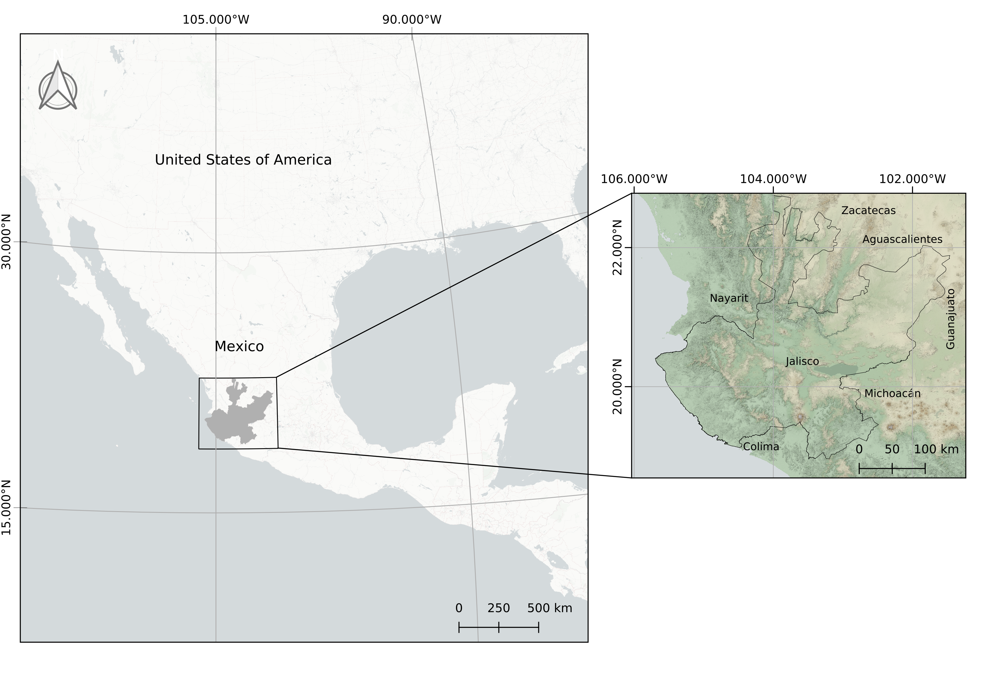
Figure 1: Study area: Jalisco, Mexico.

3 Related works

The most common use of deep learning in the classification of satellite images is using high-quality images and low number of classes such as images EUROSAT (10 classes) [12] or LandCoverNet (7 classes) [13] based on sentinel-2 (10 m spatial resolution). Our work is different from them according to the following aspects:

1. Jalisco data is more diverse, not only with more classes but also, have a wide range of LC and LU over the region. These characteristics have been shown that could affect the class separability [5].

2. We use low spatial resolution images mainly Lansat8 images with 30 m of spatial resolution, in contrast to sentinel-2 spatial resolution (10 m).

3. Our real-world base map is semiautomatic-labeled using the methodology [14] and this requires considerable efforts to obtain a reliable accuracy for the Jalisco region the overall accuracy is 89.48%.

4. We use a large number of channels combining satellite bands and terrain data. At the present, most of the DL architectures use three channels (RGB) and usually are pre-trained with IMAGENET dataset. The deep (number of layers) of those networks are incompatible with the objective of monitoring the MMU.

5. The multi-seasonal data from Landsat 8 has a coarse temporal resolution due to the cloud cover.

6. Usually, most LC datasets were created with big homogeneous generic areas (water vs non-water, forest vs. non-forest). This is because, at global extents, classes are heterogeneous internally, and merging them becomes necessary for achieving reasonable accuracies [5, 15]. It is important to remark that these characteristics are not compatible with the heterogeneous distribution of Jalisco’s region an either with LC regional requirements.

Regarding the classification performance, in our opinion, the fairest comparison of our results is the approach proposed by the MAD-MEX methodology [16]. Due to they used 12 classes and Landsat 8 images. However, it is important to note that they used a combination of Segmentation for Object-Based Image Analysis (OBIA) and traditional machine learning techniques. The overall accuracy reported from that paper is 76 %. In addition, it is important to give context about the typical performance values. According to [17] the accuracy assessment in the MAD-MEX methodology, the tropical evergreen forest was very accurately classified when the accuracy $>$ 75 %; moderate results were obtained for the tropical deciduous forest when the accuracy is around 70 %, and temperate forest categories were classified poorly (accuracy indices ranging from 50 % to 60 %).

4 Data

4.1 LULC map 2016

We use the land use cover map from Jalisco 2016 [18] which is public and can be consulted here. This map was developed jointly by the National Forestry Commission of Mexico (CONAFOR) and the Jalisco State Government. The resulting 2016 map is composed of 24 thematic categories besides, accuracy was evaluated following the methodology proposed by Olofsson [14] with an overall accuracy of 89.48 $\pm$ 0.2%.

4.2 Landsat 8 cloud-free

We use Landsat 8 data from January 1 to December 31, 2016, were collected through Google Earth Engine (GEE)[19], the preprocessing script is available at the following link. The cloud-free composite was generated by filtering the images by the values of the quality layer, where Normalized Difference Vegetation Index (NDVI) and Normalized Difference Water Index (NDWI) by applying formulas 1 and 2 on the corresponding bands.

$$NDVI=\frac{NIR-RED}{NIR+RED}$$ (1)

$$NDWI=\frac{NIR-SWIR}{NIR+SWIR}$$ (2)

where $NIR$, $NDWI$, $SWIR$ and $RED$ are defined in Table 1.

Channel	Data
1	Band 2 (BLUE) SR 0.452-0.512 $\mu m$
2	Band 3 (GREEN) SR 0.533-0.590 $\mu m$
3	Band 4 (RED) SR 0.636-0.673$\mu m$
4	Band 5 (NIR near infrared) SR 0.851-0.879 $\mu m$
5	Band 6 (SWIR Shortwave infrared) SR 0.636-0.673 $\mu m$
6	Band 7 (SWIR 2) SR 2.107-2.294 $\mu m$
7	NDVI = (Band 5 – Band 4) / (Band 5 + Band 4)
8	NDWI = (Band 6 – Band 5) / (Band 6 + Band 5)

Table 1: Landsat8 channels. Where SR = Surface Reflectance.

4.3 Relief data

A digital elevation model was included which was obtained through the portal of the National Institute of Statistics and Geography (INEGI) with a spatial resolution of 30 meters, additionally, from this data, we derived the slope, aspect, tangential and profile curvature. The GRASS software [20] was used for this purpose.

4.4 Base line dataset

Landsat 8, relief and LULC map 2016 (Labels) data were stacked into a single dataset (13 channels) an example of the data normalized can be seen in Figure 2. The name of each channel is detailed in Table 2. In addition, the name of each 17 LULC map 2016 class is presented in Table 3, the reduction in the number of class from 24 to 17 is due to the fact that the categories of permanent and perennial agriculture are merged, as is the case for induced and cultivated grassland. Another 5 categories were not considered as they were already well represented in the landscape.

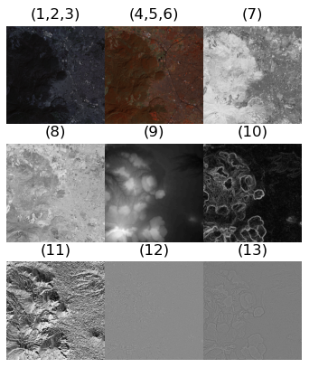
Figure 2: Example of the staked dataset image channels. We enumerate the number of the channels at the top of each image.

The approach for patch creation was to take only $3\times 3\times 13$ pixel groups where all pixels belong to a single category, under this approach to achieve a balanced sample with an equal number of elements it was necessary to reduce the number of classes to be analyzed to 17 (see Table 3), this resulted in a total of 21,046 patches with 13 channels, further divided into 70 % for training, 15 % for validation and 15 % for test.

Channel	Data
1	Lsat8 Band 2 (BLUE)
2	Lsat8 Band 3 (GREEN)
3	Lsat8 Band 4 (RED)
4	Lsat8 Band 5 (NIR near infrared)
5	Lsat8 Band 6 (SWIR Shortwave infrared)
6	Lsat8 Band 7 (SWIR 2)
7	Lsat8 NDVI = (Band 5 – Band 4) / (Band 5 + Band 4)
8	Lsat8 NDWI = (Band 6 – Band 5) / (Band 6 + Band 5)
9	Relief DEM: Digital elevation model
10	Relief Slope: Slope - Degress
11	Relief Aspect - Degress
12	Relief Tangencial Curvature
13	Relief Profile Curvature

Table 2: Band or channel used in the Baseline dataset. Lsat8 = Landsat8.

Index	ID	Class
0	32	Water
1	2	Coniferous forest
2	1	Upland coniferous forest
3	3	Oak forest and riparian forest
4	7	Cloud forest and low evergreen forest
5	9	Mangrove and peten
6	15	Crassicaule schrub
7	5	Mezquital and submontane shrub
8	34	Cultivated and induced grasslands
9	28	Natural grasslands
10	12	Tropical dry forest
11	13	Tropical semideciduous forest
12	31	Bare land
13	29	Rain fed agriculture
14	35	Cropland irrigated
15	30	Urban areas
16	26	Hydrophilic halophilic vegetation

Table 3: Land cover and land use classes used as base-line.

5 LUCC Lightweight ConvNet

The proposed ConvNet architectures and their hyperparameters were designed taking into account, the following:

1. Classify the LC using MMU.

2. The possibility to handle 2D signal with 13 channels

3. Light weights to reduce the inference and training time.

To solve these requirements we combine our experience with an expert-knowledge, tests and image analysis to select the most appropriate architecture. As a result, we propose ConvNet architecture presented in Figure 3. In this novel ConvNet we propose an input shape of $3\times 3\times 13$. In consequence, it is possible to classify the MMU. Following, we use two convolution layers with 128 and 64 filters (a wide architecture), with window size of $1\times 1$ and ReLU as activation function. The $1\times 1$ convolution is used as channel-wise pooling to promote promote learning across channels such as [21, 22, 23] and help us to handle and learn using the 13 channels. After the ConvNet layers, a Batch-normalization layer have added [24] to reduce the internal covariate shift problem, in fact, we expect to have this problem due to the study area having small-distributed examples unevenly across its territory. Then, following the flatten layer, we decide to add three dense (fully connected) layer [128,32,16] with ReLU, each one have a Gaussian dropout (30%) to reduce the overfitting [25].

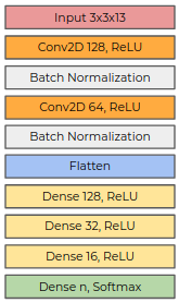
Figure 3: The proposed lightweight LUC ConvNet architecture.

6 Experimental setup

We made three trainings with the proposed architecture: i) a base-line train using a dataset with 17 balanced-classes, presented at Table 3, ii) coarse-grain training, due to embedded analysis, bring to light that eighth classes could be grouped into four, reducing to 13 classes iii) fine-grain training for binary classification in each group (with similar classes). The hyperparameters values in all the training are: learning rate= 0.0001, epochs= 150 and batch size= 32. In addition, we used 0-$90^{o}$ random rotations, horizontal and vertical flips as data augmentation.

The embedded analysis is based on a embedded layer replacing the last two layers in our CNN architecture for a embedded layer consists of an output dimension of 17 and an L2 normalization (See Figure  4). Once the model is trained, we apply a t-distributed stochastic neighbor embedding (t-SNE) [26] on the latent ConvNet representation.

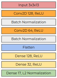
Figure 4: The proposed lightweight LUC ConvNet architecture form embedded analysis.

7 Results and analysis

The base-line test-loss and test-accuracy (using 17 classes) are 0.81 and 0.73 respectively (using the test data split). The details of the base-line classification performance per class are presented in Table 4. We observe that class-ID 32 (water) has the best classification performance with 0.96 of F1-score. In contrast, the id-classes 2,3,12,15,28,29,34 and 35 has the worst classification values in range of f1-score values from 0.35 to 0.75. In addition, the confusion matrix presented at Table 5 help us to detect the most frequent error class.

The proposed analysis using the embedding representation is presented at Figure 5. By visualizing in 2D, could be see how useful are the representations learned by ConvNet to distinguish between the classes in familiar and new domains. In this 2D representation, we can observe the presence of category clusters formed by the classes [(index = 1: class ID =2 Coniferus forest),(index 3 : ID 3 Oak forest)], [(index 8 : ID 34 cultivated grassland), (index 10 : ID 12 Tropical dry forest)] , [(index 13: ID 29 rain feed agriculture),(index 14 : ID 35 cropland irrigated)], [(index 6, ID 15 crassicaule scrub) (index 9: ID 28 natural grassland)]. As a result, we decide to create new four groups: g1=(ID 2, ID 3), g2=(ID 34, ID12), g3=( ID 29, ID 35), and g4=(ID 15, ID 28).

Precision	Recall	F1-score	Support	ID	Class
0.98	0.93	0.96	207	32	Water
0.60	0.46	0.52	185	2	Coniferous forest
0.89	0.95	0.92	210	1	Upland coniferous forest
0.42	0.30	0.35	180	3	Oak forest and riparian forest
0.69	0.81	0.75	196	7	Cloud forest and low evergreen forest
0.93	0.99	0.96	169	9	Mangrove and peten
0.60	0.85	0.71	183	15	Crassicaule schrub
0.89	0.76	0.82	192	5	Mezquital and submontane shrub
0.45	0.48	0.46	168	34	Cultivated and induced grasslands
0.43	0.36	0.39	185	28	Natural grasslands
0.59	0.58	0.58	183	12	Tropical dry forest
0.74	0.94	0.83	206	13	Tropical semideciduous forest
0.74	0.69	0.72	183	31	Bare land
0.60	0.47	0.52	191	29	Rain fed agriculture
0.76	0.74	0.75	170	35	Cropland irrigated
0.79	0.84	0.81	177	30	Urban areas
0.80	0.88	0.84	172	26	Hydrophilic halophilic vegetation

Table 4: Base-line classification report over the 17 classes.

32	2	1	3	7	9	15	5	34	28	12	13	31	29	35	30	26	ID
192	0	0	0	0	1	0	0	1	1	6	0	1	3	0	1	1	32
0	85	6	29	36	0	3	0	4	3	10	7	0	1	1	0	0	2
0	0	200	0	10	0	0	0	0	0	0	0	0	0	0	0	0	1
0	28	0	54	15	0	4	0	31	15	12	16	2	3	0	0	0	3
0	8	14	4	158	0	0	0	0	0	0	7	1	0	4	0	0	7
0	0	0	0	0	167	0	0	0	0	2	0	0	0	0	0	0	9
0	1	0	2	0	0	156	0	0	16	1	0	1	6	0	0	0	15
0	2	0	0	0	0	16	145	0	1	3	0	0	0	4	0	21	5
0	3	0	9	1	1	6	0	80	25	15	9	10	8	1	0	0	34
0	4	4	13	0	0	45	0	19	67	3	0	2	23	3	2	0	28
0	5	0	12	1	4	6	1	16	4	106	21	4	1	2	0	0	12
0	0	0	3	3	1	0	0	0	0	5	194	0	0	0	0	0	13
1	1	0	2	0	0	0	1	6	6	6	2	127	3	1	14	13	31
2	2	0	0	0	0	13	3	18	14	4	4	4	89	20	17	1	29
0	2	0	1	4	2	7	0	4	2	6	1	4	6	125	5	1	35
0	0	0	0	0	1	3	2	0	2	2	0	11	5	3	148	0	30
0	0	0	0	0	2	0	11	0	0	0	0	4	1	1	1	152	26

Table 5: Base-line confusion matrix, using 17 classes.

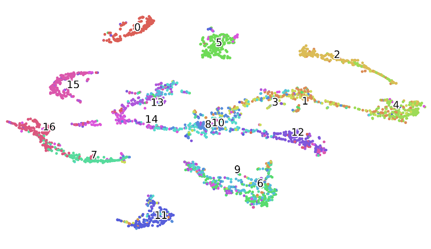
Figure 5: Embedding representation of the base-line training. The closer groups are g1=[(index = 1: class ID =2 Coniferus forest)(index 3 : ID 3 Oak forest)], g2 = [(index 8 : ID 34 cultivated grassland) (index 10 : ID 12 Tropical dry forest)] , g3=[(index 13: ID 29 rain feed agriculture)(index 14 : ID 35 cropland irrigated)], g4=[(index 6, ID 15 crassicaule scrub) (index 9: ID 28 natural grassland)].

The results of the coarse-grain classification with 13 classes (using the same ConvNet) shows lower test-loss value, 0.53, and higher test-accuracy, 0.83 in comparison base-line classification (with the 17 classes). The coarse-grain classification details are presented at Table 6. Note that the four groups increase their performance substantially. As expected, the coarse-grain confusion matrix presented at Table 7 shows noteworthy differences in the diagonal. As a result, the same model in coarse-grain classification has fewer classification mistakes.

Precision	Recall	F1-score	Support	ID	Class
0.97	0.97	0.97	152	32	Water
0.83	0.98	0.90	199	1	Upland coniferous forest
0.85	0.81	0.83	192	7	Cloud forest and low evergreen forest
0.74	0.70	0.72	184	g1	Coniferus forest and Oak forest
0.64	0.52	0.57	170	g2	Cultivated grassland and Tropical dry forest
0.83	0.62	0.71	186	g3	Rain feed agriculture and Cropland irrigated
0.70	0.86	0.77	184	g4	Crassicaule scrub and Natural grassland
0.97	1.00	0.98	190	9	Mangrove and peten
0.87	0.87	0.87	193	5	Mezquital and submontane shrub
0.83	0.95	0.88	202	13	Tropical semideciduous forest
0.82	0.73	0.77	173	31	Bare land
0.83	0.87	0.85	190	30	Urban areas
0.89	0.88	0.88	200	26	Hydrophilic halophilic vegetation

Table 6: Classification report of coarse-grain (with grouped classes).

32	1	7	g1	g2	g3	g4	9	5	13	31	30	26	ID
148	0	0	0	0	1	0	0	0	0	2	0	1	32
0	196	3	0	0	0	0	0	0	0	0	0	0	1
0	30	155	4	0	0	0	0	0	3	0	0	0	7
0	7	17	128	12	3	8	0	2	6	0	1	0	g1
0	0	3	30	88	2	6	2	2	27	9	1	0	g2
0	0	2	2	7	115	42	0	2	0	0	13	3	g3
0	4	0	6	6	6	158	0	1	0	0	3	0	g4
0	0	0	0	0	0	0	190	0	0	0	0	0	9
0	0	0	0	2	1	11	0	168	0	0	0	11	5
0	0	2	0	7	0	0	2	0	191	0	0	0	13
2	0	0	1	14	3	2	0	0	4	126	15	6	31
0	0	0	0	1	6	0	1	1	0	14	166	1	30
2	0	0	1	1	1	0	1	17	0	2	0	175	26

Table 7: Coarse-grain confusion matrix report.

The corresponding test-loss and test-accuracy are: g1 loss= 0.55, acc= 0.70, g2 loss= 0.38, acc= 0.85, g3 loss= 0.35, acc= 0.86 and g4 loss= 0.45, acc= 0.80. The fine-grain classification details over the four groups are presented in Table 8. We observe from this table that the g1 group (2: Coniferous forest, 3:Oak forest) has the lowest classification performance. In Table 9 we present the confusion matrices of each group. The values are barely in line with the classification report.

Precision	Recall	F1-score	Support	ID	Class
0.72	0.64	0.68	184	2	Coniferous forest
0.68	0.76	0.72	188	3	Oak forest
0.83	0.87	0.85	190	34	Cultivated grassland
0.86	0.82	0.84	182	12	Tropical dry forest
0.88	0.82	0.85	182	29	Rain feed agriculture
0.84	0.89	0.86	190	35	Cropland irrigated
0.84	0.75	0.79	194	15	Crassicaule scrub
0.76	0.84	0.80	178	28	Natural grassland

Table 8: Fine-grain classification report per group.

2	3	ID	34	12	ID	29	35	ID	15	28	ID
118	66	2	166	24	34	150	32	29	146	48	15
46	142	3	33	149	12	21	169	35	28	150	28

Table 9: Fine-grain confusion matrix.

In Figure 6 is presented a ground truth map and the prediction in the Guadalajara urban area using the coarse-grain data model. It is possible to note that the urban area is relatively well classified, in contrast, this model had a lower performance to discriminate between the land cover classes. It is possible to see some salt and paper artifacts in the prediction, this artifacts are related with the mask size mainly.

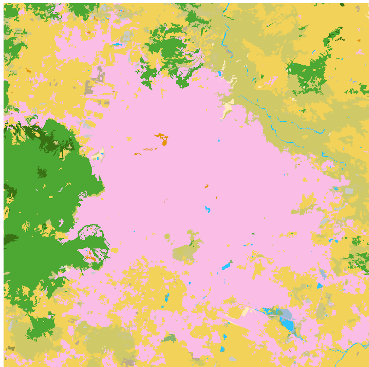
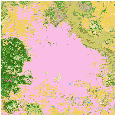
Figure 6: Left: Ground truth map of the urban area of Guadalajara. Right: prediction over the same area.

8 Discussion

Generally speaking, the results and analysis presented in the previous section indicate that the classification performance are competitive taking into account the context: number of classes (the number of classes usually have a stronger impact in the classification performance as the number of classes increases [15]), low spatial resolution (30 m), multiseasonal data, noisy labels (89% of accuracy). Regarding to classification performance, our overall classification with 13 (and 17) classes outperforms the 75% and according to to [17] this could be considered as very accurate result. In addition, the reported accuracy is achieved without any additional post-processing by experts, which is still a common practice in LULC map making a slow and costly process.

The importance of the embedded analysis is not only that this help to increase the classification performance (if the similar classes are grouped), but also, reveal the most difficult classes where the human photo-interpretation could be more critical.

About the fine-grain classification we find that our worst classification result with g1: Coniferus forest and Oak forest, there other works which have been reported previosly confusion between these two classes

9 Conclusions and Future work

In this paper we have presented a novel lightweight ConVnet to classify the LULC images combining real-world open data sources: Lansat8 (multi-seasonal and low spatial resolution) cloud-free, realief, and 2016 Jalisco’s LULC map. In contrast, to most common works, the proposed ConvNet can handle 13 channels due to $1\times 1$ convulution take into account the relation over the channels allowing to define $3\times 3$ a minimum mapeable unit of landsat8 images which is useful in the context of landcover clasification. After an embedded analysis, of the base-line results, we group the similar classes increase the test-accuracy performance from 0.73 to 0.83. The open challenges of the proposed methos are the salt and paper noise in the prediction and the lower classification performance with the groped classes.

In our opinion, these results represent an excellent initial step toward automatic LUC image classification. Our research possibly supports the decision-makers providing evidence, for example, of deforestation or forest degradation. In our opinion, the main value of our work lies in the fact that we obtain good classification performance using real-world data sources. We hope that this method could be useful by other regions and groups with limited data sources or computational resources. It is important to remark that our investigations into this area are still in progress and we hope to focus on exploring the combination with other deep learning methods such as [27, 28] to increase the performance and make robust classification.

References

- [1] Guillermo Martínez Pastur, Ajith H Perera, Urmas Peterson, and Louis R Iverson. Ecosystem services from forest landscapes: an overview. Ecosystem Services from Forest Landscapes, pages 1–10, 2018.
- [2] Yan Gao, Alexander Quevedo, Zoltan Szantoi, and Margaret Skutsch. Monitoring forest disturbance using time-series modis ndvi in michoacán, mexico. Geocarto International, 36(15):1768–1784, 2021.
- [3] Janet Franklin, Josep M Serra-Diaz, Alexandra D Syphard, and Helen M Regan. Global change and terrestrial plant community dynamics. Proceedings of the National Academy of Sciences, 113(14):3725–3734, 2016.
- [4] Mas Jean-François, Richard Lemoine-Rodríguez, Rafael González-López, Jairo López-Sánchez, Andrés Piña-Garduño, and Evelyn Herrera-Flores. Land use/land cover change detection combining automatic processing and visual interpretation. European Journal of Remote Sensing, 50(1):626–635, 2017.
- [5] Mirela G Tulbure, Patrick Hostert, Tobias Kuemmerle, and Mark Broich. Regional matters: On the usefulness of regional land-cover datasets in times of global change. Remote Sensing in Ecology and Conservation, 2021.
- [6] Ava Vali, Sara Comai, and Matteo Matteucci. Deep learning for land use and land cover classification based on hyperspectral and multispectral earth observation data: A review. Remote Sensing, 12(15):2495, 2020.
- [7] Victor Alhassan, Christopher Henry, Sheela Ramanna, and Christopher Storie. A deep learning framework for land-use/land-cover mapping and analysis using multispectral satellite imagery. Neural Computing and Applications, pages 1–16, 2019.
- [8] Prasad S Thenkabail. Remote Sensing Handbook; Volume 1: Remotely Sensed Data Characterization, Classification, and Accuracies. Taylor & Francis, 2016.
- [9] Ioannis Manakos and Matthias Braun. Land use and land cover mapping in europe. Springer London, 18:411, 2014.
- [10] Julien Radoux and Pierre Defourny. Automated image-to-map discrepancy detection using iterative trimming. Photogrammetric Engineering & Remote Sensing, 76(2):173–181, 2010.
- [11] Hermes Ulises Ramírez Sánchez, Ángel Reinaldo Meulenert Peña, and José Antonio Gómez Reyna. Actualización del atlas bioclimático del estado de jalisco. Investigaciones Geográficas, Boletín del Instituto de Geografía, 2013(82):66–92, 2013.
- [12] Patrick Helber, Benjamin Bischke, Andreas Dengel, and Damian Borth. Eurosat: A novel dataset and deep learning benchmark for land use and land cover classification. IEEE Journal of Selected Topics in Applied Earth Observations and Remote Sensing, 12(7):2217–2226, 2019.
- [13] Hamed Alemohammad and Kevin Booth. Landcovernet: A global benchmark land cover classification training dataset. arXiv preprint arXiv:2012.03111, 2020.
- [14] Pontus Olofsson, Giles M Foody, Martin Herold, Stephen V Stehman, Curtis E Woodcock, and Michael A Wulder. Good practices for estimating area and assessing accuracy of land change. Remote Sensing of Environment, 148:42–57, 2014.
- [15] Felix Abramovich and Marianna Pensky. Classification with many classes: challenges and pluses. Journal of Multivariate Analysis, 174:104536, 2019.
- [16] Steffen Gebhardt, Thilo Wehrmann, Miguel Angel Muñoz Ruiz, Pedro Maeda, Jesse Bishop, Matthias Schramm, Rene Kopeinig, Oliver Cartus, Josef Kellndorfer, Rainer Ressl, et al. Mad-mex: Automatic wall-to-wall land cover monitoring for the mexican redd-mrv program using all landsat data. Remote Sensing, 6(5):3923–3943, 2014.
- [17] Jean-François Mas, Stéphane Couturier, Jaime Paneque-Gálvez, Margaret Skutsch, Azucena Pérez-Vega, Miguel Angel Castillo-Santiago, and Gerardo Bocco. Comment on gebhardt et al. mad-mex: automatic wall-to-wall land cover monitoring for the mexican redd-mrv program using all landsat data. remote sens. 2014, 6, 3923–3943. Remote Sensing, 8(7):533, 2016.
- [18] CONAFOR and SEMADET. Mapa de Cobertura del Suelo del Estado de Jalisco al año base 2016 [Vector]. Escala 1:75,000. Versión 1.3. México, 2020.
- [19] Noel Gorelick, Matt Hancher, Mike Dixon, Simon Ilyushchenko, David Thau, and Rebecca Moore. Google earth engine: Planetary-scale geospatial analysis for everyone. Remote Sensing of Environment, 2017.
- [20] GRASS Development Team. Geographic Resources Analysis Support System (GRASS GIS) Software, Version 7.2. Open Source Geospatial Foundation, 2017.
- [21] Min Lin, Qiang Chen, and Shuicheng Yan. Network in network. arXiv preprint arXiv:1312.4400, 2013.
- [22] Christian Szegedy, Wei Liu, Yangqing Jia, Pierre Sermanet, Scott Reed, Dragomir Anguelov, Dumitru Erhan, Vincent Vanhoucke, and Andrew Rabinovich. Going deeper with convolutions, 2014.
- [23] Kaiming He, Xiangyu Zhang, Shaoqing Ren, and Jian Sun. Deep residual learning for image recognition, 2015.
- [24] Sergey Ioffe and Christian Szegedy. Batch normalization: Accelerating deep network training by reducing internal covariate shift. CoRR, abs/1502.03167, 2015.
- [25] Alex Labach, Hojjat Salehinejad, and Shahrokh Valaee. Survey of dropout methods for deep neural networks. arXiv preprint arXiv:1904.13310, 2019.
- [26] Geoffrey Hinton and Sam T Roweis. Stochastic neighbor embedding. In NIPS, volume 15, pages 833–840. Citeseer, 2002.
- [27] E Ulises Moya-Sánchez, Sebastià Xambó-Descamps, Abraham Sánchez Pérez, Sebastián Salazar-Colores, and Ulises Cortés. A trainable monogenic convnet layer robust in front of large contrast changes in image classification. IEEE access, 9:163735–163746, 2021.
- [28] Zahid Younas Khan and Zhendong Niu. Cnn with depthwise separable convolutions and combined kernels for rating prediction. Expert Systems with Applications, 170:114528, 2021.