Josephson junction-based axion detection through resonant activation
Abstract
We discuss the resonant activation phenomenon on a Josephson junction due to the coupling of the Josephson system with axions. We show how such an effect can be exploited for axion detection. A nonmonotonic behavior, with a minimum, of the mean switching time from the superconducting to the resistive state versus the ratio of the axion energy and the Josephson plasma energy is found. We demonstrate how variations in switching times make it possible to detect the presence of the axion field. An experimental protocol for observing axions through their coupling with a Josephson system is proposed.
I Introduction
Very recently the dark-matter axion detection has become a promising and fruitful research field Nagano et al. (2021); Berlin et al. (2021); Alesini et al. (2021); Wang et al. (2021); Chaudhuri (2021); Backes et al. (2021); Battye et al. (2020); Arvanitaki et al. (2020); Braine et al. (2020); Buschmann et al. (2020); Nagano et al. (2019); Malnou et al. (2019); Du et al. (2018); Brubaker et al. (2017).
Josephson systems are recognized of paramount importance as a sensitive experimental tool, as a playground for many theoretical models, and for their applications in fast, low-noise electronics Barone and Paterno (1982); Devoret et al. (1984); Devoret and Schoelkopf (2013); Guarcello et al. (2015); Nogueira et al. (2016); Tafuri (2019); Irastorza and Redondo (2018); Braginski (2019); Kjaergaard et al. (2020); Lee et al. (2020); Walsh et al. (2021); Rettaroli et al. (2021); Guarcello et al. (2017).
In the last years, a Josephson junction
(JJ) has been supposed to interact with axions, the hypothetical elementary particles proposed as a possible component of cold dark matter Dixit et al. (2021); Murayama (2007); Bradley et al. (2003), by exploiting
the matching between the energies of the axion and the JJ Beck (2013, 2017); Yan and Beck (2020). Very recently, hard X-ray emission from neutron stars has been explained by axion
emission Dessert et al. (2020); Malte Buschmann
et al. (2021). The axion’s mass estimation is compatible with the values postulated by the Peccei-Quinn theory introduced in 1977 to solve
the strong CP problem in quantum chromodynamics Peccei and Quinn (1977). The theory introduces a new scalar field which spontaneously breaks the symmetry at
low energies, giving rise to an axion that suppresses the CP violation Co et al. (2020); Chang and Cui (2020). Moreover, unexplained events in Josephson-based experiments Hoffmann et al. (2004); Bae et al. (2008); He et al. (2011); Golikova et al. (2012); Bretheau et al. (2013)
can be well justified on the basis of the axion-JJ coupling. This hypothesis has thus paved the way to think of JJs as possible axion-detectors. However, up
to now, no systematic investigations of resonance experimental conditions, suitable for direct Josephson-based axion detection, have been carried out.
Here, we consider a Josephson-based detector to exploit the measurable voltage drop that appears across the device when the combined
action of bias current and thermal fluctuations induces the switch from the superconducting to the resistive state Piedjou Komnang et al. (2021); Guarcello et al. (2021, 2017, 2019). In the presence of
axion coupling, the analysis of the mean switching times (MST), , for the JJ reveals the occurrence of a resonance effect.
This is the axion-induced resonant activation phenomenon
characterized by a nonmonotonic behavior of , with a minimum, versus the ratio of the axion to the Josephson plasma energy.
Furthermore, our work allows the identification of the suitable experimental conditions for a Josephson system to effectively detect such an axion-JJ resonance.
Based on these findings, an experimental procedure for observing axions coupled to a JJ system is proposed.
The paper is organized as follows. The physical characteristics and the mathematical formalism of the two subsystems, JJ and axion, and the composed axion-JJ system are presented in Secs. II, III and IV, respectively. In Sec. V, the axion-induced resonant activation phenomenon is discussed in detail, while in Sec. VI the outlines of two possible experimental schemes are proposed. Finally, conclusive remarks are reported in Sec. VII.
II RCSJ Model
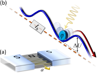
We consider a superconductor-normal metal-superconductor JJ (see Appendix A.1), Fig. 1(a), whose phase dynamics can be described within the resistively and capacitively shunted junction (RCSJ) model Barone and Paterno (1982); Guarcello et al. (2017, 2020); Guarcello and Bergeret (2020) as
| (1) |
The time is normalized to the inverse of the characteristic frequency, that is with .
is the maximum Josephson current that can flow through the device, while and are, respectively, the normalized external bias current and thermal noise current.
is the Stewart-McCumber parameter, with and being the normal-state resistance and
capacitance of the JJ, respectively. A JJ can be effectively described in terms of a particle moving along a washboard potential tilted by (see Appendix A.1),
see Fig. 1(b). Increasing , the slope of the washboard potential increases and the height of the confining potential barrier reduces, up to
vanish altogether for . Overdamped and underdamped JJs are characterized by and , respectively.
In this work, the random current is modeled as a standard Gaussian white noise associated to the JJ resistance, with the usual statistical properties
and . The amplitude of the normalized correlation is connected with the
physical temperature through the relation Barone and Paterno (1982)
| (2) |
III Axion field
An axion field is characterized by two parameters, the axion misalignment angle and the axion coupling constant , namely Sikivie (1983). Within the Robertson-Walker metric, which is appropriate to describe the early universe, the homogeneous equation of motion of the axion misalignment angle reads Co et al. (2020)
| (3) |
Here, is the Hubble parameter and denotes the axion
mass.
It is evident the similarity between the equations of motion governing the axion and the RCSJ systems: the axion dynamics is analogous to that of a RCSJ
with no externally applied bias current. Besides the formal mathematical analogy between the two systems, it is physically remarkable that the parameters
characterizing the two equations are quite similar as their order of magnitude is concerned (see Appendix A.2).
IV Axion-JJ System
The interaction between axion and JJ can be formally written as
| (4a) | ||||
| (4b) | ||||
where and are the dissipation and frequency parameters, respectively; is the coupling constant between axion and JJ and its value can be inferred from experimental quantities Yan and Beck (2020). In analogy to what happens in resonant cavities, the axion-JJ coupling is supposed to be responsible for the decay of the axion into two photons, one of which (that characterized by a vanishing moment) generates electron-hole pairs which in turn create a supercurrent Dixit et al. (2021); Murayama (2007); Bradley et al. (2003); Beck (2013).
By considering the presence of both a bias current and thermal fluctuations in the JJ equation, the axion-JJ system [Eqs. (4)] can be conveniently rewritten as (see Appendix B)
| (5a) | ||||
| (5b) | ||||
with
| (6) |
where is the Josephson plasma frequency. We assume that the additional sinusoidal term depending on in Eq. (5a) can be ascribed to the Cooper-pair current indirectly induced by the axion entering the junction. In other words, the axion induces an extra current term. The parameter indicates the ratio between the axion energy and the Josephson plasma energy, , and represents our “control knob” to set the most convenient working point for the detection of an axion field interacting with the JJ. Indeed, the Josephson plasma frequency, and therefore the energy ratio , can be “adjusted” as needed, since can be lowered by raising the temperature Dubos et al. (2001), applying a magnetic field Bergeret and Cuevas (2008) or a gate voltage Du et al. (2008); De Simoni et al. (2019). In this way, the system response can be tuned to achieve a working regime in which the switching dynamics of the axion-JJ coupled system well deviates from the Josephson response in the absence of axions. This condition makes the axion-JJ interaction clearly detectable.
Now we analyze how the axion affects the MST, i.e. the average time the JJ system takes to switch from the initial superconducting state (particle at the bottom of the well) to the resistive state. Due to random thermal fluctuations, the particle can escape from the potential well, even if the junction is biased by a current below the critical value (i.e., ). According to Kramers’ theory, in the strong damping limit the average escape rate from a neighbouring potential barrier in the presence of a noise source, with intensity expressed by Eq. (2), is given in the simplest approximation by the following expression Guarcello et al. (2020)
| (7) |
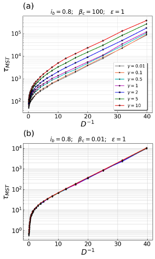
In Fig. 2 we show the behavior of the normalized MST, , as a function of the inverse of the noise intensity, ,
under different damping conditions, performing independent numerical realizations from Eqs. (5). The linear behavior of
vs characterizes a Kramers-like law. We note that if we multiply Eq. (4a) by , the latter appears only
in the second-derivative terms, while the first-derivative term will be multiplied by the square root of . Consequently, under the overdamped approximation
() the coupling term becomes negligible with respect to all the other terms in Eq. (4a)
and the two equations decouple, as it is evident by comparing the two panels in Fig. 2. Therefore,
a suitable regime for the JJ system to detect axions is the underdamped regime ().
Furthermore, the axion-coupling induces only a shift of the curves upwards as the coupling parameter increases, while the slope is substantially
unchanged (Fig. 2). Therefore, only the prefactor of the Kramers-like law is influenced by and not the height of the effective
potential barrier Graham and Tél (1985); Kautz (1996), which is given by the slope of the curves of Fig. 2(a).
V Resonant activation effect
In light of the above result, it is interesting to study the dependence of the MST on the ratio between the axion energy
and the Josephson plasma energy. We further emphasize that the Josephson energy depends on the plasma frequency and, therefore, it can be tuned in
experiments. However, the energy cannot be lowered at will, for example it is always necessary to ensure that the intensity of the thermal fluctuations is much lower
than the critical current of the junction.
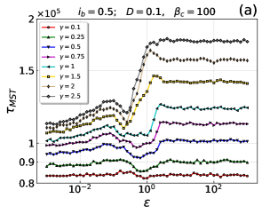
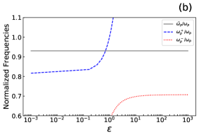
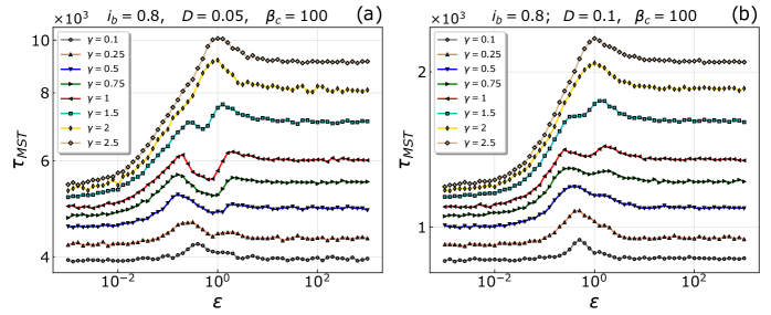
Figure 3(a) clearly shows a significant nonmonotonic behavior of vs , with a minimum in the range , which is a signature of an axion-JJ resonant activation phenomenon, observed in JJs both in the absence and presence of a noise source Devoret et al. (1984); Guarcello et al. (2015); Doering and Gadoua (1992). This resonant phenomenon is ascribed to the frequency-matching condition between the frequency associated to the axion angle field and the JJ plasma frequency (see Appendix B). In fact, the term in Eq. (5a) can be interpreted as an oscillating current for the Josephson system, which is responsible for the resonant activation phenomenon Devoret et al. (1984); Guarcello et al. (2015). The minimum is less pronounced for low and high values of . In particular, for low values of the coupling parameter, , the minimum is affected by the decoupling, which smoothes the curve towards a constant behavior; for high coupling values, , very high values of , due to the confinement of the JJ phase particle (), tend to shallow the minimum. In the intermediate range, the minimum is more pronounced showing the resonant activation phenomenon. Indeed, by linearizing Eqs. (4), in the absence of noise, we get in the underdamped regime the expression for the frequency associated with the axion-JJ system (see Appendix B)
| (8) |
with
| (9) |
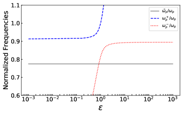
The frequency matching between and the effective plasma frequency occurs at [see Fig. 3(b)], just close to the position of the minimum in the curves of vs in Fig. 3(a). The resonant matching condition
is robust enough to be observed with a different set of parameter values (see Appendix B).
Furthermore, the position of this local minimum depends on both the coupling parameter and the applied bias current , and moves towards lower
values of for higher values of . For low values of the resonant effect is more visible [Fig. 3(a)], while for higher bias
values it tends to disappear as increases (see Appendix B). At low noise intensity, the resonant effect is still present, and even more evident (see Appendix B).
Moreover, for and , the curves approach two different plateaux. For , the two equations describing the dynamics
of the two systems, JJ and axion, decouple, since the effects of on in Eq. (5a) are due to the term
. For , the oscillations of are highly damped, so as to compensate the high values of .
This can be seen in Eq. (5b) where the term is responsible for the sinusoidal shape of the potential felt by the
axion. For the potential well is extremely deep so that the axion oscillations are narrowly confined.
Furthermore, due to the term , which is always opposite to the bias term, the total effective current becomes smaller than (results
not shown). This feature indicates that the presence of an axion tends to confine the effective phase particle representing the JJ system behavior. This explains why the value of
the MST tends to increase for .
Thus, the two plateaux at low and high are somewhat different when , while for lower
couplings the two plateaux are practically at the same level. In fact, for the weight of the term is lessened by the presence
of , which vanishes if tends to zero and the axion-JJ equations decouple. Therefore, in the region a MST
that deviates significantly from the expected unperturbed value () represents, together with the presence of the minimum, a hallmark of an axion-JJ interaction and therefore of the axion detection.
The comparison between the MST measurements in the unperturbed case (1), predicted also by
Kramers theory, and those obtained for can lead to an estimate of .
In particular, first the behaviour of the MST as a function of the parameter is obtained.
Afterwords, through a comparison of the theoretical curves shown in Figs. 3(a) and 4 with the experimental one, the value of the coupling parameter can be determined.
The observation that higher values of give higher
values of the MST, both for and for , is well justified too. In fact, since effectively behaves as a current
term in Eq. (5a), a stronger axion-JJ coupling results in an effective lower bias current which further confines the Josephson phase particle.
This confinement, therefore, is due to both a greater axion-JJ coupling constant and a greater energy ratio .
This therefore identifies the suitable experimental conditions for a JJ-based axion detection. First, as the MST analysis is concerned, it has been shown that
the underdamped regime is suitable to highlight the axion-induced effects on the JJ dynamics. Second, it has been found that for any value of the coupling parameter,
according to the axion-mass estimates Beck (2013, 2017), it is convenient to tune the plasma frequency, through the critical current, to reach the limit .
This allows an improved estimate of the parameter , thanks to the greatest spacing between the curves related to different values of the axion-JJ coupling
for . This makes the values of compatible with the experimental range of more easily detectable for . Third, and
most importantly, we have found a resonant activation phenomenon due to the frequency matching condition in the transition range .
The energy of the dark matter axion is estimated in the energy range . To fulfill the condition requires
a suitable JJ device with a sufficiently low critical current , which can be even further reduced by heating and/or magnetic fields. Therefore, although the value of
is not known precisely, it is still possible to design a setup to control its variation. This makes possible to range from the almost decoupled working
regime () to the well coupled one ().
VI Possible Experimental Setup
Based on the results previously shown, a technique to setup an experiment to detect the axion field is here outlined. First, as the parameter depends on the JJ critical current , Eq. (6), by tuning it is possible to measure the MST deviation from the dynamical regime characterized by high (which entails small and for which the axion signal is ineffective) to that characterized by low (which entails large and for which the axion signal is effective). Thus, as the critical current of the JJ is decreased, for instance by means of a magnetic field, the effects described by Eqs. (5) become more and more evident [see Fig. 3(a)] in the same experimental set-up. Finally, by tuning the frequency matching condition to observe the resonant phenomenon, the axion should be revealed.
Another possible experimental setup is to consider many JJs with significantly different critical currents and to
observe an increase in the MSTs when the critical current passes the condition , that is, after Eq.(6), .
Again, a tuning of the resonant matching condition should reveal the axion.
We note that the increase in Fig. 3(a) is observed in normalized units;
the relation between the actual () and the normalized () average switching times also depends on the critical current:
, according to the normalization of Eq. (13). In other words, as increases due to the decrease in , the
amplification effect on the non-normalized MSTs should be even greater than that shown in Fig. 3(a).
VII Conclusions
We have investigated the MSTs of a JJ directly coupled to an axion field and subject to both a dc bias current and thermal fluctuations. We have found the experimental conditions for a JJ-based axion detection: a) the underdamped regime; b) a Josephson plasma energy lower than the axion energy; c) the axion-induced resonant activation phenomenon, due to the occurrence of an effective frequency matching between axion and JJ, when the ratio of the axion energy to that of the junction falls in the range . Furthermore, an experimental strategy for a JJ-based axion detection is proposed.
Perhaps most importantly, we propose to reveal the axion presence through the analysis of the escape times from the superconducting initial state. Thus, studying the switching time statistics, we have found a resonant activation phenomenon, based on the plasma frequency, induced on the JJ by the axion that turns out to act as an effective time-dependent oscillating bias current.
Finally, our approach can be applied to different physical scenarios, like damped pendula, two capacitively coupled JJs Blackburn et al. (2009), excitable coupled JJs Hens et al. (2015) and coupled qubits architectures for quantum computing Krantz et al. (2019); Grønbech-Jensen et al. (2010), paving the way to further theoretical achievements and new technological applications.
Acknowledgements.
Acknowledgments. This work was supported by Italian Ministry of University and Research (MIUR) and the Government of the Russian Federation through Agreement No. 074-02-2018-330 (2).Appendix A
A.1 RCSJ Model
A short tunnel JJ is a quantum device formed by sandwiching a thin insulating layer between two superconducting electrodes, in which both lateral dimensions are smaller than the Josephson penetration depth Barone and Paterno (1982). The dynamics of the Josephson phase for a dissipative, current-biased short JJ can be studied within the RCSJ model Barone and Paterno (1982); Guarcello et al. (2015); Spagnolo et al. (2017) that in non-normalized units can be written as
| (10) |
Here, is the washboard potential along which the phase evolves,
| (11) |
where . The resulting activation energy barrier, , confines the phase in a metastable potential minimum and can be calculated as the difference between the maximum and minimum value of . In units of , it can be expressed as
| (12) |
In the phase particle picture, the term represents the tilting of the potential profile; increasing the slope of the washboard increases and the height of the right potential barrier reduces, until this activation energy vanishes for , that is when the bias current reaches its critical value .
If one normalizes the time to the inverse of the characteristic frequency, that is with , Eq. (10) can be put in the dimensionless form
| (13) |
where is the Stewart-McCumber parameter. Usually, the single-harmonic current-phase relation (CPR) is appropriate to describe the features of a JJ Golubov et al. (2004), i.e., the high-order harmonic terms can be neglected. However, we observe that a non-sinusoidal CPR, as in the case of a short SNS junction Beenakker (1992), is not expected to undermine the feasibility of the Josephson-based scheme for axion detection discussed in this work, but only to slightly affect the specific switching time values. An overdamped junction has , that is a small capacitance and/or a small resistance. In contrast, a junction with has a large capacitance and/or a large resistance, and is underdamped. Another way to obtain a dimensionless form of Eq. (10) consists in normalizing with respect to the plasma frequency . In this case the normalized RCSJ equation (10) reads
| (14) |
where is the damping parameter and . With this time normalization the under- and over-damped regimes correspond to and , respectively.
We note that normalizing with respect to the characteristic frequency , as we did in our numerical simulations, the noise intensity can be simply expressed as the ratio of thermal energy to Josephson coupling energy , or , without any dependence on the damping. Normalizing instead with respect to the plasma frequency , the noise intensity becomes .
In our numerical simulations, for Gaussian fluctuations of amplitude , the stochastic independent increment reads
| (15) |
Here, the symbol indicates a random function Gaussianly distributed with zero mean and unit standard deviation. The stochastic integration of Eqs. (13) or (14) is performed with a finite-difference explicit method, using a time integration step .
A.2 Axion paramaters
An axion field can be formally written as Sikivie (1983); Visinelli (2013), where is the axion misalignment angle and the axion coupling constant. The axion’s misalignment angle dynamics obeys the following homogeneous equation of motion Co et al. (2020)
| (16) |
where denotes the axion mass and the Hubble parameter. The typical ranges of parameters that are allowed for dark matter axions are Sikivie and Yang (2009); Duffy and van Bibber (2009)
| (17) |
and
| (18) |
The prediction of the axion’s mass based on the average of the results obtained from five independent condensed matter experiments is Hoffmann et al. (2004); Golikova et al. (2012); He et al. (2011); Bae et al. (2008); Bretheau et al. (2013)
| (19) |
These energies values permit to estimate the corresponding values of the energy ratio , see Eq. (6). To do this, first of all the main parameters of Josephson must be set: for example, we can generically choose the values , , and for the resistance per area, the specific capacitance, and the critical current density, respectively, which gives a plasma frequency and a Stewart-McCumber parameter .
Then, from Eq. (18) we get , which is approximately the range of values we have explored in this work. Moreover, these values match the almost decoupled working regime () and the well coupled one (), at which the vs curves approach two different plateaux. Finally, the average value in Eq. (19) corresponds to an energy ratio , i.e., a value just close to the resonant matching condition discussed in Sec. V.
Appendix B Linearization and Frequency Matching Condition
The interaction model proposed for a coupled axion-JJ system reads [Eqs. (4) of the main text]
| (20a) | |||
| (20b) | |||
where is the coupling parameter. In the presence of both a bias and a stochastic current, by normalizing with respect to the squared plasma frequency , the system (4) can be rewritten as
| (21a) | |||
| (21b) | |||
with
| (22a) | ||||
and the term proportional to can be neglected, since
| (23) |
Normalizing with respect to the characteristic frequency , the system of differential equations becomes
| (24a) | |||
| (24b) | |||
with .
In this work, by numerically solving Eqs. (5), we report the calculation of the MST as a function of the energy ratio . Specifically, in Fig. 4 the curves of MST versus are shown for a higher bias value, , with respect to that shown in Fig. 3(a) of the main text and for two noise intensity values, namely and . These curves show that the resonant phenomenon tends to disappear for higher bias values and that it is still present and more evident at low noise intensity. Indeed, the resonant activation phenomenon is observed in the presence and in the absence of a noise source, see Refs. Devoret et al. (1984); Guarcello et al. (2015); Doering and Gadoua (1992) (and references therein).
Let us consider the limit of small oscillations for both the JJ and the axion, in the absence of a noise source. In this case, we can approximate and in Eqs. (5). The resulting linearized system reads
| (25a) | ||||
| (25b) | ||||
with and . In the overdamped regime (), the first term can be neglected in both equations. By adding and subtracting the two equations, we obtain
| (26a) | ||||
| (26b) | ||||
which implies
| (27a) | ||||
| (27b) | ||||
Therefore, the two equations describing the dynamics of the two systems decouple. This indicates that the overdamped linearized regime is unsuitable for axion detection.
In the underdamped regime the normalization with respect to allows to more easily interpret the frequency-matching phenomenon.
Indeed, by putting (underdamped regime) in Eqs. (21) and neglecting the noisy fluctuating current term, the linearized system, this time, remains coupled
| (28a) | ||||
| (28b) | ||||
The analytical solutions, for the initial conditions considered in the main text, namely , are
| (29a) | ||||
| (29b) | ||||
where
| (30a) | ||||
| (30b) | ||||
| (30c) | ||||
| (30d) | ||||
In Fig. 5 we show the behavior of the frequencies , in units of , as a function of at and . The black solid line indicates the bias-dependent plasma frequency . In Eq. (5), the term can be considered as an oscillating drive, with two specific characteristic frequencies given by . Therefore, a resonant effect on the switching dynamics is expected when one of the two characteristic frequencies of the oscillating drive and the Josephson plasma frequency match. This is the resonant activation phenomenon observed both in the absence and in the presence of a noise source Devoret et al. (1984); Guarcello et al. (2015). In particular, in Fig. 5 it is shown the expected frequency matching at , that is just close to the position of the central minimum in the curves of vs in Fig.2 of the main text. Here, the frequency matching is with and the parameter values are different from those used to get the curves of Fig. 3 in the main text. This indicates that the resonant matching condition is robust enough to be observed with a different set of parameter values.
For we get the following simpler expressions
| (31a) | ||||
| (31b) | ||||
In this case, for small oscillations, the axion and the JJ are characterized by the same two frequencies: and , and the time evolutions of the two solutions appear very similar.
References
- Nagano et al. (2021) K. Nagano, H. Nakatsuka, S. Morisaki, T. Fujita, Y. Michimura, and I. Obata, Phys. Rev. D 104, 062008 (2021).
- Berlin et al. (2021) A. Berlin, R. T. D’Agnolo, S. A. R. Ellis, and K. Zhou, Phys. Rev. D 104, L111701 (2021).
- Alesini et al. (2021) D. Alesini, C. Braggio, G. Carugno, N. Crescini, D. D’Agostino, D. Di Gioacchino, R. Di Vora, P. Falferi, U. Gambardella, C. Gatti, et al., Phys. Rev. D 103, 102004 (2021).
- Wang et al. (2021) J.-W. Wang, X.-J. Bi, and P.-F. Yin, Phys. Rev. D 104, 103015 (2021).
- Chaudhuri (2021) S. Chaudhuri, Journal of Cosmology and Astroparticle Physics 2021, 033 (2021).
- Backes et al. (2021) K. M. Backes, D. A. Palken, S. A. Kenany, B. M. Brubaker, S. B. Cahn, A. Droster, G. C. Hilton, S. Ghosh, H. Jackson, S. K. Lamoreaux, et al., Nature 590, 238 (2021).
- Battye et al. (2020) R. A. Battye, B. Garbrecht, J. I. McDonald, F. Pace, and S. Srinivasan, Phys. Rev. D 102, 023504 (2020).
- Arvanitaki et al. (2020) A. Arvanitaki, S. Dimopoulos, M. Galanis, L. Lehner, J. O. Thompson, and K. Van Tilburg, Phys. Rev. D 101, 083014 (2020).
- Braine et al. (2020) T. Braine, R. Cervantes, N. Crisosto, N. Du, S. Kimes, L. J. Rosenberg, G. Rybka, J. Yang, D. Bowring, A. S. Chou, et al. (ADMX Collaboration), Phys. Rev. Lett. 124, 101303 (2020).
- Buschmann et al. (2020) M. Buschmann, J. W. Foster, and B. R. Safdi, Phys. Rev. Lett. 124, 161103 (2020).
- Nagano et al. (2019) K. Nagano, T. Fujita, Y. Michimura, and I. Obata, Phys. Rev. Lett. 123, 111301 (2019).
- Malnou et al. (2019) M. Malnou, D. A. Palken, B. M. Brubaker, L. R. Vale, G. C. Hilton, and K. W. Lehnert, Phys. Rev. X 9, 021023 (2019).
- Du et al. (2018) N. Du, N. Force, R. Khatiwada, E. Lentz, R. Ottens, L. J. Rosenberg, G. Rybka, G. Carosi, N. Woollett, D. Bowring, et al. (ADMX Collaboration), Phys. Rev. Lett. 120, 151301 (2018).
- Brubaker et al. (2017) B. M. Brubaker, L. Zhong, Y. V. Gurevich, S. B. Cahn, S. K. Lamoreaux, M. Simanovskaia, J. R. Root, S. M. Lewis, S. Al Kenany, K. M. Backes, et al., Phys. Rev. Lett. 118, 061302 (2017).
- Barone and Paterno (1982) A. Barone and G. Paterno, Physics and applications of the Josephson effect (Wiley, New York, 1982).
- Devoret et al. (1984) M. H. Devoret, J. M. Martinis, D. Esteve, and J. Clarke, Phys. Rev. Lett. 53, 1260 (1984).
- Devoret and Schoelkopf (2013) M. H. Devoret and R. J. Schoelkopf, Science 339, 1169 (2013).
- Guarcello et al. (2015) C. Guarcello, D. Valenti, and B. Spagnolo, Phys. Rev. B 92, 174519 (2015).
- Nogueira et al. (2016) F. S. Nogueira, Z. Nussinov, and J. van den Brink, Phys. Rev. Lett. 117, 167002 (2016).
- Tafuri (2019) F. Tafuri, Fundamentals and Frontiers of the Josephson Effect, vol. 286 (Springer, Cham, Switzerland, 2019).
- Irastorza and Redondo (2018) I. G. Irastorza and J. Redondo, Progress in Particle and Nuclear Physics 102, 89 (2018).
- Braginski (2019) A. I. Braginski, Journal of Superconductivity and Novel Magnetism 32, 23 (2019).
- Kjaergaard et al. (2020) M. Kjaergaard, M. E. Schwartz, J. Braumüller, P. Krantz, J. I.-J. Wang, S. Gustavsson, and W. D. Oliver, Annual Review of Condensed Matter Physics 11, 369 (2020).
- Lee et al. (2020) G.-H. Lee, D. K. Efetov, W. Jung, L. Ranzani, E. D. Walsh, T. A. Ohki, T. Taniguchi, K. Watanabe, P. Kim, D. Englund, et al., Nature 586, 42 (2020).
- Walsh et al. (2021) E. D. Walsh, W. Jung, G.-H. Lee, D. K. Efetov, B.-I. Wu, K.-F. Huang, T. A. Ohki, T. Taniguchi, K. Watanabe, P. Kim, et al., Science 372, 409 (2021).
- Rettaroli et al. (2021) A. Rettaroli, D. Alesini, D. Babusci, C. Barone, B. Buonomo, M. M. Beretta, G. Castellano, F. Chiarello, D. Di Gioacchino, G. Felici, et al., Instruments 5, 022915 (2021).
- Guarcello et al. (2017) C. Guarcello, D. Valenti, B. Spagnolo, V. Pierro, and G. Filatrella, Nanotechnology 28, 134001 (2017).
- Dixit et al. (2021) A. V. Dixit, S. Chakram, K. He, A. Agrawal, R. K. Naik, D. I. Schuster, and A. Chou, Phys. Rev. Lett. 126, 141302 (2021).
- Murayama (2007) H. Murayama, in Particle Physics and Cosmology: The Fabric of Spacetime, edited by F. Bernardeau, C. Grojean, and J. Dalibard (Elsevier, 2007), vol. 86 of Les Houches, pp. 287–347.
- Bradley et al. (2003) R. Bradley, J. Clarke, D. Kinion, L. J. Rosenberg, K. van Bibber, S. Matsuki, M. Mück, and P. Sikivie, Rev. Mod. Phys. 75, 777 (2003).
- Beck (2013) C. Beck, Phys. Rev. Lett. 111, 231801 (2013).
- Beck (2017) C. Beck, PoS EPS-HEP2017, 058 (2017).
- Yan and Beck (2020) J. Yan and C. Beck, Physica D: Nonlinear Phenomena 403, 132294 (2020).
- Dessert et al. (2020) C. Dessert, J. W. Foster, and B. R. Safdi, The Astrophysical Journal 904, 42 (2020).
- Malte Buschmann et al. (2021) M. Malte Buschmann, R. T. Co, C. Dessert, and B. R. Safdi, Physical Review Letters 126, 021102 (2021).
- Peccei and Quinn (1977) R. D. Peccei and H. R. Quinn, Phys. Rev. Lett. 38, 1440 (1977).
- Co et al. (2020) R. T. Co, L. J. Hall, and K. Harigaya, Phys. Rev. Lett. 124, 251802 (2020).
- Chang and Cui (2020) C.-F. Chang and Y. Cui, Phys. Rev. D 102, 015003 (2020).
- Hoffmann et al. (2004) C. Hoffmann, F. Lefloch, M. Sanquer, and B. Pannetier, Phys. Rev. B 70, 180503 (2004).
- Bae et al. (2008) M.-H. Bae, R. C. Dinsmore III, M. Sahu, H.-J. Lee, and A. Bezryadin, Phys. Rev. B 77, 144501 (2008).
- He et al. (2011) L. He, J. Wang, and M. H. Chan, arXiv preprint arXiv:1107.0061 (2011).
- Golikova et al. (2012) T. E. Golikova, F. Hübler, D. Beckmann, I. E. Batov, T. Y. Karminskaya, M. Y. Kupriyanov, A. A. Golubov, and V. V. Ryazanov, Phys. Rev. B 86, 064416 (2012).
- Bretheau et al. (2013) L. Bretheau, Ç. Ö. Girit, H. Pothier, D. Esteve, and C. Urbina, Nature 499, 312 (2013).
- Piedjou Komnang et al. (2021) A. Piedjou Komnang, C. Guarcello, C. Barone, C. Gatti, S. Pagano, V. Pierro, A. Rettaroli, and G. Filatrella, Chaos Solitons Fract 142, 110496 (2021), ISSN 0960-0779.
- Guarcello et al. (2021) C. Guarcello, A. S. Piedjou Komnang, C. Barone, A. Rettaroli, C. Gatti, S. Pagano, and G. Filatrella, Phys. Rev. Applied 16, 054015 (2021).
- Guarcello et al. (2019) C. Guarcello, D. Valenti, B. Spagnolo, V. Pierro, and G. Filatrella, Physical Review Applied 11, 044078 (2019).
- Guarcello et al. (2020) C. Guarcello, G. Filatrella, B. Spagnolo, V. Pierro, and D. Valenti, Physical Review Research 2, 043332 (2020).
- Guarcello and Bergeret (2020) C. Guarcello and F. Bergeret, Phys. Rev. Applied 13, 034012 (2020).
- Sikivie (1983) P. Sikivie, Phys. Rev. Lett. 51, 1415 (1983).
- Dubos et al. (2001) P. Dubos, H. Courtois, B. Pannetier, F. K. Wilhelm, A. D. Zaikin, and G. Schön, Phys. Rev. B 63, 064502 (2001).
- Bergeret and Cuevas (2008) F. S. Bergeret and J. C. Cuevas, Journal of Low Temperature Physics 153, 304 (2008).
- Du et al. (2008) X. Du, I. Skachko, and E. Y. Andrei, Phys. Rev. B 77, 184507 (2008).
- De Simoni et al. (2019) G. De Simoni, F. Paolucci, C. Puglia, and F. Giazotto, ACS Nano 13, 7871 (2019).
- Graham and Tél (1985) R. Graham and T. Tél, Phys. Rev. A 31, 1109 (1985).
- Kautz (1996) R. L. Kautz, Reports on Progress in Physics 59, 935 (1996).
- Doering and Gadoua (1992) C. R. Doering and J. C. Gadoua, Phys. Rev. Lett. 69, 2318 (1992).
- Blackburn et al. (2009) J. A. Blackburn, J. E. Marchese, M. Cirillo, and N. Grønbech-Jensen, Physical Review B 79, 054516 (2009).
- Hens et al. (2015) C. Hens, P. Pal, and S. K. Dana, Physical Review E 92, 022915 (2015).
- Krantz et al. (2019) P. Krantz, M. Kjaergaard, F. Yan, T. P. Orlando, S. Gustavsson, and W. D. Oliver, Applied Physics Reviews 6, 021318 (2019).
- Grønbech-Jensen et al. (2010) N. Grønbech-Jensen, J. E. Marchese, M. Cirillo, and J. A. Blackburn, Phys. Rev. Lett. 105, 010501 (2010).
- Spagnolo et al. (2017) B. Spagnolo, C. Guarcello, L. Magazzú, A. Carollo, D. Persano Adorno, and D. Valenti, Entropy 19 (2017).
- Golubov et al. (2004) A. A. Golubov, M. Y. Kupriyanov, and E. Il’ichev, Rev. Mod. Phys. 76, 411 (2004).
- Beenakker (1992) C. W. J. Beenakker, in Low-Dimensional Electronic Systems, edited by G. Bauer, F. Kuchar, and H. Heinrich (Springer Berlin Heidelberg, Berlin, Heidelberg, 1992), pp. 78–82.
- Visinelli (2013) L. Visinelli, Modern Physics Letters A 28, 1350162 (2013).
- Sikivie and Yang (2009) P. Sikivie and Q. Yang, Physical Review Letters 103, 111301 (2009).
- Duffy and van Bibber (2009) L. D. Duffy and K. van Bibber, New Journal of Physics 11, 105008 (2009).