Enabling Deep Learning on Edge Devices through Filter Pruning and Knowledge Transfer

Abstract

Deep learning models have introduced various intelligent applications to edge devices, such as image classification, speech recognition, and augmented reality. There is an increasing need of training such models on the devices in order to deliver personalized, responsive, and private learning. To address this need, this paper presents a new solution for deploying and training state-of-the-art models on the resource-constrained devices. First, the paper proposes a novel filter-pruning-based model compression method to create lightweight trainable models from large models trained in the cloud, without much loss of accuracy. Second, it proposes a novel knowledge transfer method to enable the on-device model to update incrementally in real time or near real time using incremental learning on new data and enable the on-device model to learn the unseen categories with the help of the in-cloud model in an unsupervised fashion. The results show that 1) our model compression method can remove up to 99.36% parameters of WRN-28-10, while preserving a Top-1 accuracy of over 90% on CIFAR-10; 2) our knowledge transfer method enables the compressed models to achieve more than 90% accuracy on CIFAR-10 and retain good accuracy on old categories; 3) it allows the compressed models to converge within real time (three to six minutes) on the edge for incremental learning tasks; 4) it enables the model to classify unseen categories of data (78.92% Top-1 accuracy) that it is never trained with.

1 Introduction

Deep neural networks (DNNs) have been applied to many important applications on edge devices, such as image classification, speech recognition, and augmented reality. These deep learning models typically have millions of parameters and need to be trained for hours or even days on powerful cloud servers to achieve a good performance. However, a serious drawback of this cloud-only approach is that the on-device tasks cannot perform well when the cloud is overloaded or the network is unreliable. Moreover, there are also significant benefits from training deep leaning models on edge devices: 1) Customization: user- or situation-specific requirements can be met more effectively by training models on the devices that the users or physical environments directly interact with; 2) Responsiveness: custom models deployed on devices for specific users or environments can better adapt to their changing behaviors using new data captured by the devices; and 3) Privacy: sensitive information can be better protected if the sensitive data and models are stored and used only on private devices, not in the public resources shared by many.

Deploying and training complex deep learning models on edge devices are challenging since they require millions of parameters and large amounts of operations whereas the devices have only limited memory and computation resources. To deploy DNNs on resource-constrained devices, there are two general approaches. The first approach aims to compress already-trained models, using techniques such as weights sharing (Chen et al., 2015), quantization (Han et al., 2015; Kadetotad et al., 2016), and pruning (Han et al., 2015; LeCun et al., 1990; Srinivas & Babu, 2015). However, a compressed model generated by these approaches is useful only for inference; it cannot be re-trained to capture user- or device-specific requirements or new data available at runtime.

The second approach to learning on devices is based on knowledge transfer which uses the knowledge distilled from a cloud-based deep model (termed teacher) to improve the accuracy of a on-device small model (termed student) (Ba & Caruana, 2014; Hinton et al., 2015; Romero et al., 2014; Venkatesan & Li, 2016). However, these works 1) achieve limited accuracy improvement (Yim et al., 2017; Zagoruyko & Komodakis, 2016); 2) do not consider the speed of training the model to a satisfactory accuracy; and 3) assume that the all data are available at the training time and the tasks for the student and teacher remain exactly the same, which is often not a realistic assumption.

The goal of our work is to provide a new solution that allows deep learning models to be trained on devices with a small number of parameters, the state-of-the-art accuracy, and fast runtime. Further, we aim to enable on-device learning under realistic settings where the models are trained incrementally with only limited local input but are still able to recognize both old and new categories of data.

In order to achieve the above goal, we propose a new compression method for deploying models that are suitable and trainable for resource-constrained devices, and a new knowledge transfer method for improving the training accuracy and the speed of these on-device models, and providing the capability for enabling the on-device models to learn incrementally without forgetting the knowledge on the old categories using the local data and achieve good accuracy for classifying both old and new categories. Specifically, our compression method can create a model that is both shallow and thin by removing similar convolution layers and pruning filters that produce weak activation patterns in each layer, respectively, from a large model trained in the cloud. The resulting compressed model still shares the same architecture as the original model, and is suited for knowledge transfer between the two models. Our proposed knowledge transfer method selects the best teacher/student layer pairs for transferring knowledge from teacher’s intermediate representations and enables the student to learn the problem solving process. Our proposed method also enables the student to use the distilled knowledge from the teacher in solving the catastrophic forgetting problem.

We evaluate our solution on VGG-16 and ResNet architectures using CIFAR-10, Caltech 101, and ImageNet datasets. First, our model compression method 1) reduces 99.36% parameters of WRN-28-10, while preserving a Top-1 accuracy of over 90% on CIFAR-10; and 2) achieves a compression ratio of up to 139X on VGG-16, at a cost of less than 10% accuracy loss on Caltech 101. Second, our knowledge transfer method 1) enables the compressed models not only perform well on new category ($>$90% accuracy on CIFAR-10) but also retains a good level of accuracy for classifying the old categories; and 2) enables the compressed models to converge within real time (three to six minutes) on the edge for incremental learning tasks; and 3) allows the compressed model to reach a Top-1 accuracy of 78.92% on CIFAR-10 for classifying unseen categories that it is never trained with. Compared to the related works (Romero et al., 2014; Zagoruyko & Komodakis, 2016), our method reduces complex networks to both shallower and thinner networks without much loss of accuracy, enables the models to learn from new categories incrementally within real time without forgetting the old categories, and allows the models to classify unseen categories of data with both good accuracy and speed.

In summary, our solution enables DNNs that are not only suitable for deployment on resource-constrained devices but also trainable for meeting new requirements. In the rest of the paper, we first explain the details of our proposed solution (Section 2), then present an extensive evaluation (Section 3), discuss the related works (Section 4), and finally conclude the paper (Section 5).

2 Background and Motivations

We envision an edge computing scenario where edge devices collect various data (voice, images, videos, etc.) from their sensors and feed it to the cloud. In the cloud, we can utilize the abundant resources in the cloud to train a state-of-the-art model with all the available data. On the edge, we can deploy a small model on each device and train it using the local data for customized, responsive, and private learning.

In order to realize the above scenario, the cloud/edge distributed learning system needs to meet the following requirements. First, the on-device model should be small enough to fit the limited resources on the edge devices, which are usually resources constrained due to their small form factor. Second, the on-device models should be able to classify new categories without forgetting old categories since re-training the whole model on edge devices is infeasible due to their limited computing resources. Third, the on-device model should be able to classify unseen categories with good accuracy, since each edge device may only see a subset of the data that the cloud model is trained with.

To meet the above requirements, we need to use compression techniques to produce models that are small enough and fast enough for the edge devices with their limited resources. We also need knowledge transfer techniques that can utilize the knowledge of the in-cloud model to help the on-device models retain the existing knowledge while learning on new data and be able to classify categories that they are not trained with.

But on one hand, existing model compression methods focused only on creating compressed models for efficient inference without considering how to compression methods affect the training process (Han et al., 2015; Chen et al., 2015; Kadetotad et al., 2016; Li et al., 2016; Polino et al., 2018), and how to reduce the accuracy loss caused by compression. On the other hand, existing knowledge transfer methods have the following limitations: 1) they still require large student models that are not fit for resources constrained devices (Romero et al., 2014; Li et al., 2019; Yim et al., 2017); 2) they only enable to student model to classify the categories that the models are trained with.

To address these limitations and meet the aforementioned requirements, we propose novel model compression and knowledge transfer techniques for deploying models that are suitable and trainable for resource-constrained devices and improving the training accuracy and speed of these on-device models, as detailed in the rest of the paper.

3 Filter Pruning Based Model Compression

Without loss of generality, we consider image classification tasks and use ResNet, as an example to discuss our proposed on-device learning solution. Image classification is important for many edge applications, and is also the target task of the related model compression and knowledge distillation works (Hinton et al., 2015; Han et al., 2015; Chen et al., 2015; Polino et al., 2018; Srinivas & Babu, 2015). ResNet is a modern architecture with streamlined convolutional layers. Specifically, we consider WRN-28-10 and ResNet-34, illustrated as Teacher in Figure 2. They have a Top-1 accuracy of 97.28% on CIFAR-10 and 73.9% on ImageNet, respectively, which are among the state-of-the-art results. The ResNet models consist of several groups of blocks, and each block has two convolutional layers. Further, we also consider VGG-16 (Simonyan & Zisserman, 2014), which is another commonly used neural network and has a different architecture, including 13 convolutional layers and three fully-connected layers.

Our goal for model compression is two-fold: 1) to reduce the number of parameters and optimize the architecture of the model so that it is both thin and shallow, and fit for the limited resources on a device; 2) to maintain the architecture of the original model so that it can facilitate the learning from the on-server model during knowledge transfer.

The proposed model compression method works as follows. First, to reduce depth, it creates a shallower model that has the same number of groups as the on-server model, but each group only keeps the last block (illustrated as Student in Figure 2). This way of pruning layers of a model also resonates with the principle that higher layer features are closer to the useful features for performing a main task (Yim et al., 2017). Next, our method reduces the width of the shallower model by removing filters that produce weak activation patterns. It uses one batch of images to decide the number of filters that are safe to prune in each convolution layer.

The procedure of pruning filters from the $i$th convolution layer is as follows. For a given input image m, let $X^{m}_{i-1}$ denote the input features of the $i$th convolution layer. Convolution operations (denoted as mapping function $F$) transform the input $X_{i-1}^{m}$ into output feature maps $Z_{i}^{m}$ by applying $n_{i}$ three-dimensional filters $f_{i,j}^{m}$. Then, activation operations (denoted as mapping function $G$) transform $Z_{i}^{m}$ into the activation feature maps $A_{i}^{m}$:

$$Z_{i}^{m}=F(X_{i-1}^{m}),\quad A_{i}^{m}=G(Z_{i}^{m})$$ (1)

For each filter’s activation feature map $a^{m}_{i,j}\in R^{h_{i}\times w_{i}}$ ($1\leq j\leq n^{i}$), our method computes the percentage of zero elements based on the $l_{0}$-norm of $a^{m}_{i,j}$:

$$perc(a^{m}_{i,j})=1-\frac{{\|a^{m}_{i,j}\|}_{0}}{h^{i}\times w^{i}}.$$ (2)

If the percentage is equal to or greater than Filter Pruning Threshold $P$, this filter is safe to be pruned. The threshold determines how aggressive the pruning is, and in the evaluation, we set it between 0.7 and 1.0. Our method repeats the above procedure for M randomly selected images, and calculates the average number ($avgc_{i}$) of filters that are safe to prune. We set $M$ equal to batch size since we find that the value of $avgc_{i}$ is steady even if the input features are different. The reduced width $w^{i}$ of the $i$th convolution layer becomes: $w^{i}=n^{i}-avgc_{i}$. The same method is applied to all the remaining layers of the shallow model. The model is then retrained with the reduced width and depth to generate the compressed on-device model.

We can visualize the activations of the on-server model (WRN-28-10) on CIFAR-10 and understand why our filter pruning method is effective. Figure 1 shows the activation feature maps of each filter of the first convolutional layer (called Conv1) using one image as the input. The width of Conv1 is $16$. The first image on the left is the original image, and the second image is the input features after data augmentation. We can see that some filters extract lots of representations with high activation patterns, like the $6$th and $12$th filters, whereas the activation feature maps of some filters are close to zero, such as the $2$nd, $14$th, and $16$th filters. Filters that generate weak activations are safe to remove without affecting the final performance of the model.

In this way, we can generate a compressed model that is both shallow and thin, small enough for learning on edge devices. The small model still shares the same architecture of the original model, because it retains the higher layers in each group of convolutional layers and keeps important filters in each remaining layers. Compared to the related filter pruning work that prunes filters with the lowest absolute weight sum (Li et al., 2016), our approach prunes insignificant filters more accurately. Filters that have small absolute weight sum can also produce useful non-zero activation patterns that are important for learning features during backpropagation. As shown in Table 1 of Section 5.1, our method enables the compressed model achieving a higher Top-1 test accuracy than their method (93.68% vs 93.55%), with a smaller number of parameters (1.42M vs 1.68M). So our approach directly finds and prunes the filters that generate close-to-zero activations, with minimal impact on the performance.

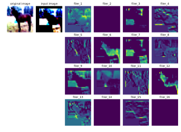
Figure 1: Activation feature maps of each filter of the first convolutional layer (Conv1) of the on-server model (WRN-28-10) on CIFAR-10. In the left, the first image shows the original image and the second image shows the input features after data augmentation; the right part shows activation features of the 16 filters.

4 Selective Layer-Wise Knowledge Transfer

4.1 Knowledge Transfer for Incremental Learning on the Edge

As new local input becomes available to a device, we want to update its local model to learn the new data. One solution is to wait for the in-cloud model to update using all the data from the edge and then compress and download the updated model, which however will take a significant amount of time. In order to update the on-device model in real time or near real time, we propose to update it incrementally using its new data, and use knowledge transfer from the in-cloud model (the teacher) to preventing the on-device model (the student) from forgetting the old data that it is already trained with.

Different from the existing works (Kim et al., 2018; Romero et al., 2014; Zagoruyko & Komodakis, 2016), with our knowledge transfer method, the student does not need to learn the specific output from the teacher, which depends on the specific input; it instead learns the problem solving process, which represents the intermediate layer outputs. Learning from the teacher’s intermediate representations is better than learning from only the last layer’s output (Sharma et al., 2018), which prevents the model from losing its classification ability when facing specific questions.

Figure 2 illustrates the architecture of our knowledge transfer method for ResNet and VGG-16. The student is trained by knowledge transfer between selected teacher-student layer pairs as the input enters batch by batch at each iteration. First, given one batch of data, our method finds out which convolutional blocks in the teacher should be used to transfer knowledge to the student’s convolutional blocks, using a new cosine similarity based metric. Then, multiple loss functions are built using the activations from the mapped block pairs.

In order to find best teacher-student layer pairs for knowledge transfer, first, we define a cosine similarity metric for measuring the similarity between the activation feature maps of the teacher’s $k$th block and the student’s $j$th block:

$$CosineSim_{k,j}(X)=\frac{Q^{t}_{k}\cdot Q^{s}_{j}}{\left\|Q^{t}_{k}\right\|\left\|Q^{s}_{j}\right\|},$$ (3)

$$Q^{t}_{k}=\frac{F^{t}_{k}(X)}{\left\|F^{t}_{k}(X)\right\|},\quad Q^{s}_{j}=\frac{F^{s}_{j}(X)}{\left\|F^{s}_{j}(X)\right\|},$$ (4)

where,
$X$: one batch of data.
$F^{t}_{k}(X)$: activation feature maps of the teacher’s $k$th block.
$F^{s}_{j}(X)$: activation feature maps of the student’s $j$th block.

As shown above, the cosine similarity is calculated using $l_{2}$-normalized feature maps, which helps the student’s learning by normalizing activations of the teacher and student into a similar scope. In addition, our method does zero padding on the activation features maps of the student models before normalization, since the width of convolution layers of compressed student models is different from that of the teacher. It calculates the cosine similarity between each pair of teacher/student blocks in the same group, and the pairs $(k^{*},j^{*})$ that produce the largest cosine similarity value are mapped together for knowledge transfer.

Then the loss function is built by adding all the loss terms from intermediate layers ($J_{b}$), the fully-connected layers ($J_{1}$), and the cross entropy loss ($J_{3}$) with true labels of the dataset together, defined as follows:

$$\ell=\lambda_{1}J_{1}+\lambda_{2}\sum_{m=1}^{g}J_{b}+\lambda_{3}J_{3}$$

$$J_{1}(FC^{t},FC^{s})=\sqrt{\sum_{i=1}^{n}(FC^{t}_{i}-FC^{s}_{i})^{2}};$$

$$J_{b}(Q^{t}_{k},Q^{s}_{j})=\sqrt{\sum_{i=1}^{n}(Q^{t}_{ki}-Q^{s}_{ji})^{2}},\quad b=1,2,3,...,g;$$

$$J_{3}=\sum_{i=1}^{c}[Y_{i}log\widehat{Y_{i}^{s}}+(1-Y_{i})log(1-\widehat{Y_{i}^{s}})]$$

where,
$\qquad\lambda_{1},\lambda_{2},\lambda_{3}$: hyper-parameters to balance the weights of different loss terms
$\qquad c$: the number of classes of the datasets
$\qquad g$: the number of groups of the teacher/student
$\qquad n$: the number of feature maps of the teacher/student
$\qquad FC^{t}$: output of teacher’s last fully-connected layer
$\qquad FC^{s}$: output of student’s last fully-connected layer
$\qquad Q^{t}_{k}$: $l_{2}$-normalized output of teacher’s $k$th block
$\qquad Q^{s}_{j}$: $l_{2}$-normalized output of student’s $j$th block
$\qquad\widehat{Y^{s}}$: predicted softmax output of the student
$\qquad Y$: true labels of the datasets

Note that, as the input changes batch by batch, the mapped block pairs also change according to the cosine similarity, in order to ensure knowledge transfer is always done with the best teacher-student pairs. During backpropagation, our method only updates the weights of the last convolutional layer in each group of the student model while minimizing the loss function. This form of updating is reasonable since: 1) freezing some of the layers corresponding to the original model can help limit its adaptability to new data(Jung et al., 2016; Castro et al., 2018); 2) higher layer features are closer to the useful features for performing a main task (Yim et al., 2017); and 3) updating less layers allows the training to complete sooner on resource-constrained devices.

4.2 Knowledge Transfer for Classifying Unseen Categories on the Edge

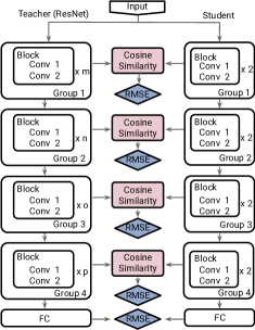
(a) Techer-Student ResNet

(b) Techer-Student VGG-16

Figure 2: Schematics of the proposed knowledge transfer method for ResNet models (on the left) and VGG-16 models (on the right).

As the in-cloud model improves over time from the data fed by the edge, there are unseen categories for the on-device models since each edge has seen only a subset of that data that the cloud is trained with. Given the data belonging to the unseen categories, the on-device model cannot classify it but the in-cloud model can. One way to solve this problem is to compress the in-cloud model and download it again to the device. Alternatively, we propose to also use the aforementioned knowledge transfer method to enable the existing model (the student) on the device to learn the unseen categories, with the help from the in-cloud model (the teacher), but without relying on data labels which may not be available to this device.

First, mapped blocks are selected in the same way as the knowledge transfer for classifying unseen categories discussed in the previous section. Next, the loss function is built by using only the mapped block pairs of all the groups ($J_{b}$) and the last fully-connected layer of the teacher and student models ($J_{1}$) from Eq. 4.1.

5 Evaluation

We implemented our solution on TensorFlow version r1.3, and elvaluated the cloud model on a Nvidia Tesla K40 GPU, hosted on a server equipped with dual Intel Xeon E5-2630 processors and 64GB of main memory. We evaluate our edge model on a commercialized device, Google Pixel 2, which has an eight-core, Qualcomm Kryo 280 CPU and 4GB of main memory. In our experiments of ResNet models, we used SGD with Nesterov momentum for optimization. Dampening was set to 0, momentum to 0.9, initial learning rate to 0.1, and mini-batch size to 128. On CIFAR-10, weight decay was set to to 0.0005, and learning rate decayed each epoch with the cosine annealing schedule, training for total 200 epochs; On ImageNet, weight decay was set to to 0.0001, and learning rate dropped by 0.1 at 30, 60, and 90 epochs, training for total 100 epochs. In the experiments of VGG-16 models, we used Adam for optimization. Initial learning rate was set to 0.01 for the original on-server model and 0.001 for compressed models. They decayed exponentially each epoch with a factor of 0.98. Validation and test accuracy of all the models were calculated at each epoch. Final accuracy of the model was reported as the test accuracy attained at the epoch with the highest validation accuracy.

We conducted experiments on three important datasets:

CIFAR-10 consists of 60,000 (32X32) RGB natural images, belonging to 10 classes with 6000 images per class (Krizhevsky et al., 2009). Each image is 32X32 pixels in 3 color channels.

Caltech 101 consists of 9145 (224X224) RGB images from 101 classes. Each class has 40 to 800 images. We divide the dataset into three parts: the training set consists of 5853 images (64% of the total dataset), the testing set consists of 1829 images (20%), and the validation set consists of 1463 images (16%) (Fei-Fei et al., 2007).

ImageNet consists of over 14 million RGB images organized into 21,841 classes. Each class has over 500 images. We use the subset of images with SIFT features, which belong to 1000 classes (Deng et al., 2009).

We preprocess all data by subtracting the mean and dividing by the standard deviation of each image vector. For experiments on CIFAR-10 and Caltech 101, all training images are padded 4 pixels on each side, and a 32X32 crop is randomly sampled from the padded image. Then the images are flipped left-right randomly with a probability of 0.5 and masked out randomly with a cutout size of 16X16 pixels (Lee et al., 2015). For experiments on ImageNet, all training images are first cropped randomly with a size of 224X224, and then horizontally flipped randomly with a given probability of 0.5.

5.1 Results for Model Compression

Table 1: Model compression results of WRN-28-10, VGG-16, and ResNet-34 on CIFAR-10, Caltech 101, and ImageNet, respectively. P denotes pruning threshold.

Data	Model	P	Accuracy	Param-	Comp.
Set	Name			eters (M)	Ratio
	WRN-28-10		97.28%	36.22
	ResNet 1	1.0	94.37%	2.00	18$\times$
CIFA-	ResNet 2	0.9	93.68%	1.42	25$\times$
R10	ResNet 3	0.8	92.62%	0.60	60$\times$
	ResNet 4	0.7	90.09%	0.23	160$\times$
	ResNet-34		73.23%	21.6
	ResNet 5	1.0	69.76%	9.79	$2\times$
Image-	ResNet 6	0.9	68.14%	7.22	$3\times$
Net	ResNet 7	0.8	66.07%	5.09	$4\times$
	ResNet 8	0.7	63.16%	3.34	$6\times$
	VGG-16		77.10%	134
	VGG-16 1	1.0	62.85%	5.55	24$\times$
Calt-	VGG-16 2	0.9	60.55%	3.78	36$\times$
ech 101	VGG-16 3	0.8	59.51%	3.11	43$\times$
	VGG-16 4	0.7	56.77%	0.97	139$\times$

We first experiment on CIFAR-10 dataset with ResNet (WRN-28-10) as the on-server model. By changing the pruning threshold P, our method can flexibly generate four compressed models, ResNet 1-4, offering different tradeoffs between size and accuracy, shown in Table 1. The results show that all the compressed models can achieve good compression ratios without losing much accuracy. In particular, compressed ResNet 4, the size of which is only 0.64% of the origin model WRN-28-10, still remains a Top-1 accuracy of over 90%. ResNet 7 achieves a compression ratio of 4X at the cost of 7.16% loss in accuracy. The compressed model VGG-16 4 achieves a compression ratio of up to 139X at the cost of less than only 10% loss in accuracy.

Table 2 shows the comparison of the proposed model compression method and the related works on CIFAR-10. The related filter pruning work (Li et al., 2016) ResNet-110-prune was evaluated on ResNet-110, and the related PM (“post-mortem”) quantilization and quantized distillation works were evaluated on WRN-28-20. Our method allows the compressed ResNet 2 (93.68%) to achieve a comparable accuracy as that of ResNet-110-pruned (Li et al., 2016) (93.55%), quantized distillation (94.73%), and a higher accuracy than PM quantization (Polino et al., 2018) (81.09%) while requiring much less parameters (1.42M) than all these four compressed models (5.4M, 1.68M, 7.44M, and 9.66M). Meanwhile, the compression ratio of compressed ResNet 2 (25X) also outperforms that of all other compressed models (3X, 1X, 19X, and 15X) significantly, achieving a much higher compression ratio and producing a much smaller model for edge deployment.

Table 2: Comparison of the proposed model compression method on CIFAR-10.

Model Name	Accuracy	Parameters (M)	Comp. Ratio
WRN-28-10	97.28%	36.22
ResNet 1	94.37%	2.00	18$\times$
ResNet 2	93.68%	1.42	25$\times$
ResNet-110	93.53%	1.72
ResNet-110-prune	93.55%	1.68	1$\times$
WRN-28-20	95.74%	145
PM Quantization	81.09%	7.44	19$\times$
Quantized Distill.	94.73%	9.66	15$\times$

5.2 Knowledge Transfer

We use on-server models (WRN-28-10 and VGG-16) as the teacher model, and their corresponding compressed models as the student model. We compare the performance of the student model that is trained with the help from the teacher, called the dependent student, with two baselines: the teacher model and the independent student model. The teacher model is used as a baseline to see how much the student represents the state-of-the-art accuracy. The independent student model is trained directly on targets without applying any form of knowledge transfer, and is used as a baseline to see how much improvement the knowledge transfer method brings to the dependent student.

Table 3: Convergence time of compressed ResNet models on CIFAR-10, and VGG-16 models on Caltech 101.

Model Name	Indepen.	Depend. (Our)	Depend. (FitNet)	Speedup (Our)	Speedup (FitNet)
ResNet 1	70.20K	12.09K	69.42K	5.81$\times$	1.01$\times$
ResNet 2	69.42K	12.87K	69.03K	5.39$\times$	1.01$\times$
ResNet 3	69.42K	15.99K	69.03K	4.34$\times$	1.01$\times$
ResNet 4	70.98K	8.97K	70.20K	7.91$\times$	1.01$\times$
VGG-16 1	8.66K	1.87K	6.08K	4.63$\times$	1.42$\times$
VGG-16 2	3.98K	3.28K	3.28K	1.21$\times$	1.21$\times$
VGG-16 3	3.28K	1.87K	3.28K	1.75$\times$	1.00$\times$
VGG-16 4	3.28K	1.87K	4.45K	1.75$\times$	0.74$\times$

5.2.1 Incremental learning

We first evaluate on the incremental learning tasks using both CIFAR-10 and ImageNet dataset with ResNet (WRN-28-10 and ResNet-34) as the teacher models, respectively. Our goal is to allow the student model, which is compressed from the teacher model, to learn one or multiple new, locally available categories without forgetting those old categories that the teacher is trained with. Re-training the whole model on edge devices is infeasible due to their limited computing resources; fine-tuning the on-device model can significantly reduce the training time, but its performance on old categories degrade severely. Our proposed method allows the teacher model to provide distilled knowledge to guide the student model and prevent it from forgetting about the old categories. In the experiment, we first pre-trained with 9 categories of data and try to learn a new category.

Table 4 lists the accuracy for incremental learning using CIFAR-10. As expected, the independent student (w/o KT) cannot classify any of the old categories any more even though it performs well on the new category. In contract, our dependent students (w/ KT) not only perform well on the new category ($>$90% accuracy) but also retains a good level of accuracy for classifying the old categories. The distilled knowledge from the teacher model significantly alleviates the catastrophic forgetting, when the student model learns the new categories incrementally. Our proposed method also works well for highly compressed models. ResNet 4 (w/ KT), with a compression ratio of 160X, achieves an accuracy only 2% lower than that of the ResNet 1 model.

We then compare our method with the related work (Li et al., 2019) by applying its knowledge transfer method to two models, ResNet d28w10, the original, uncompressed model used by RILOD, which has a compression ratio of 18X. On d28w10, RILOD’s accuracy is 7.66% lower than our ResNet 2 (w/ KT) even though it has 9.58M more parameters, indicating that our proposed method can better solve the incremental learning problem. On ResNet 1, our accuracy improvement is even more significant (20.84%). The results demonstrate that our proposed knowledge transfer method can better support incremental training on edge devices, especially for small models suited for edge deployment.

Table 5 lists the results for incremental learning on ImageNet. We sampled 10 random categories from the ImageNet dataset as our experiment dataset. We can observe similar results as the aforementioned CIFAR-10 results. The independent student (w/o KT) achieves only 11.1% accuracy on the 9 old categories after learning one new category. Our dependent student (ResNet-5 (w/ KT)) achieves 57.33% accuracy on the 9 old categories and 72% on the new category. Even the highly compressed model, ResNet 8, is only 2% less accurate than the ResNet 5 model.

Table 4: Top-1 accuracy on CIFAR-10 for single-task incremental learning using 9+1 categories of data.

Model	9 old	1 new	Avg Acc
ResNet 1 w/o KT	0	100	10
ResNet 1 (w/ KT)	62.83	93.5	78.16
ResNet 2 (w/ KT)	64.12	92.3	78.21
ResNet 3 (w/ KT)	61.5	93.1	77.3
ResNet 4 (w/ KT)	57.02	95	76.01
ResNet 1 (RILOD)	38.34	76.3	57.32
d28w10 (RILOD)	83.41	57.6	70.5

Table 5: Top-1 accuracy on ImageNet for single-task incremental learning using 9+1 categories of data.

Model	9 old	1 new	Avg Accuracy
ResNet 5 w/o KT	11.1	100	19.9
ResNet 5 (w/ KT)	57.33	72	64
ResNet 5 (RILOD)	51.78	62	56.89
ResNet-18 (RILOD)	33	98	65.5
ResNet 6 (w/ KT)	62	68	65
ResNet 7 (w/ KT)	57.7	78	67.89
ResNet 8 (w/ KT)	56.4	76	66.2

Table 6: Runtime on ImageNet for single-task incremental learning using 9+1 categories of data on the edge.

Model Name	Trainable Para.	Training Time (s)	Inference Time (s)
ResNet-18 (RILOD)	11.69	1200	8.7
ResNet 5	3.51	360	7.2
ResNet 6	3.07	315	5.3
ResNet 7	2.46	253	3.7
ResNet 8	1.76	181	2.5

In addition to improving accuracy, by using compressed models for incremental training on edge devices, our approach also runs faster than the original RILDO approach which uses a large, uncompressed model (ResNet-18) on devices. Table 6 compares the training time and inference time of our compressed ResNet models between these two approaches. Training time is measured by the total runtime required to converge, and inference time is measured by the time needed for classifying one batch of images.

All our compressed models can converge within three to six minutes on the edge whereas RILOD needs 20 minutes. In addition, the inference time of our models (from 2.5s to 7.2s) is also shorter than that of RILOD (8.7s). The above results demonstrate the importance of our model compression and knowledge transfer techniques in improving both accuracy and runtime performance of incremental learning on edge devices.

5.2.2 Classifying Unseen Categories

We then study the performance of the compressed student models when presented with data from classes that they are never trained with. In this experiment, we train our compressed ResNet models only with 10,000 images from two categories of the original training dataset (CIFAR-10), which has ten categories and 5,000 images each. Then we test them with 8,000 images from the other eight categories that they are never trained with.

Table 7 shows the accuracy of the independent student and dependent student models of classifying the unseen eight categories of images. For all of the compressed ResNet models, the accuracy of the independent students is all zero, showing that they cannot classify the unseen categories. Since they never saw those categories during training, no features were learned. However, our proposed knowledge transfer method allows the student models to achieve an accuracy of at least 60%. ResNet 1 and ResNet 2 achieve an accuracy of 78.92% and 75.72% respectively, even though they are trained with only such a small dataset including only two categories of images. FitNet cannot help in this case and its accuracy is zero on all of its dependent students. The reason is likely that FitNet learns the features generated from the teacher, instead of the process of solving a problem, so its knowledge transfer works only when the target tasks of the teacher and student models are similar.

Table 7: Top-1 accuracy of knowledge transfer methods for classifying unseen categories on CIFAR-10.

Model Name	Independent (Baseline)	Dependent (Our KT)	Dependent (FitNet)
ResNet 1	0.00%	78.92%	0.00%
ResNet 2	0.00%	75.72%	0.00%
ResNet 3	0.00%	70.40%	0.00%
ResNet 4	0.00%	61.96%	0.00%

6 Related Works

Model compression techniques can be broadly classified into three categories, weight sharing, quantization, and pruning techniques. Weight sharing reduces the occupied memory by using the same set of weights to represent more than one transformations (Han et al., 2015; Chen et al., 2015). Quantization reduces the size of the model by shrinking the number of bits needed for storing the weights (Han et al., 2015; Kadetotad et al., 2016). Pruning removes redundant weights or neurons while minimizing accuracy loss. Han proposed to remove weights below a particular threshold (Han et al., 2015). Li proposed to prune filters with the lowest absolute weight sum (Li et al., 2016). But the above related works focused only on creating compressed models for efficient inference, and did not consider how the compression methods affect the training process, and how to address the accuracy loss caused by compression. More recently, Polino et al. proposed Quantized Distillation, which leverages quantization and distillation jointly during the training process of the smaller model (Polino et al., 2018).

Existing knowledge transfer techniques can be broadly classified into three categories, including transferring hard logits, transferring soft logits, and transferring intermediate representations. Ba et al. proposed hard-logits-based knowledge transfer technique (Ba & Caruana, 2014), which minimizes squared difference (RMSE) between the logits of the teacher and the shallow student. Hinton et al. introduced transferring soft logits (Hinton et al., 2015) where the student minimizes the sum of two objective functions: (1) cross entropy loss between the soft logits, and (2) cross entropy loss between the softmax output and correct labels of the dataset. Romero et al. proposed FitNet, which extended transferring soft logits by using not only the soft outputs but also the intermediate representations learned by the teacher (Venkatesan & Li, 2016). More recently, FSP matrix transfer (Yim et al., 2017), attention transfer (Zagoruyko & Komodakis, 2016), and factor transfer (Kim et al., 2018) were proposed, which are also based on transferring the intermediate representations.

However, these knowledge transfer methods have the following limitations: 1) they still require large student models that are not fit for resource-constrained devices. For example, the student model used in RILOD (Li et al., 2019) has the same architecture with the teacher model; FitNet is thinner but not shallower, and FSP is shallower but not thinner. In comparison, we integrate proposed filter based model compression method with knowledge transfer method, enabling the student model both shallower and thinner than the teacher, which is important for deployment on resource-constrained devices; 2) they enable their student models classifying only the categories that the models are trained with, whereas our method also allows the students to classify unseen categories with a good accuracy; 3) they did not update the student incrementally in real time, whereas our method enables the students learning new categories within 181 seconds on the edge while remaining a good accuracy on the old categories.

7 Conclusions

This paper provides a novel solution to deploying and training state-of-the-art models on resourced-constrained edge devices. Our results show that, by pruning similar layers in a model and the filters that produce weak activation patterns in each layer, complex DNNs can be reduced to both shallower and thinner networks, suitable for deployment on devices but without much loss of accuracy. In addition to reducing the size, our solution allows our compressed models to converge the training within three to six minutes on the edge. Our results also show that such compressed models can also learn incrementally on new data without forgetting the old categories. In addition, our results show that transferring the problem solving process is much more effective than letting the student simply mimic teacher’s intermediate results. It allows the on-device model to be trained with both good accuracy and speed, without relying on the input’s true labels, and to recognize unseen categories.

References

- Ba & Caruana (2014) Ba, J. and Caruana, R. Do deep nets really need to be deep? In Advances in neural information processing systems, pp. 2654–2662, 2014.
- Castro et al. (2018) Castro, F. M., Marín-Jiménez, M. J., Guil, N., Schmid, C., and Alahari, K. End-to-end incremental learning. In Proceedings of the European Conference on Computer Vision (ECCV), pp. 233–248, 2018.
- Chen et al. (2015) Chen, W., Wilson, J., Tyree, S., Weinberger, K., and Chen, Y. Compressing neural networks with the hashing trick. In International Conference on Machine Learning, pp. 2285–2294, 2015.
- Deng et al. (2009) Deng, J., Dong, W., Socher, R., Li, L.-J., Li, K., and Fei-Fei, L. Imagenet: A large-scale hierarchical image database. In 2009 IEEE conference on computer vision and pattern recognition, pp. 248–255. Ieee, 2009.
- Fei-Fei et al. (2007) Fei-Fei, L., Fergus, R., and Perona, P. Learning generative visual models from few training examples: An incremental bayesian approach tested on 101 object categories. Computer vision and Image understanding, 106(1):59–70, 2007.
- Han et al. (2015) Han, S., Mao, H., and Dally, W. J. Deep compression: Compressing deep neural networks with pruning, trained quantization and huffman coding. arXiv preprint arXiv:1510.00149, 2015.
- Hinton et al. (2015) Hinton, G., Vinyals, O., and Dean, J. Distilling the knowledge in a neural network. arXiv preprint arXiv:1503.02531, 2015.
- Jung et al. (2016) Jung, H., Ju, J., Jung, M., and Kim, J. Less-forgetting learning in deep neural networks. arXiv preprint arXiv:1607.00122, 2016.
- Kadetotad et al. (2016) Kadetotad, D., Arunachalam, S., Chakrabarti, C., and Seo, J.-s. Efficient memory compression in deep neural networks using coarse-grain sparsification for speech applications. In Proceedings of the 35th International Conference on Computer-Aided Design, pp. 78. ACM, 2016.
- Kim et al. (2018) Kim, J., Park, S., and Kwak, N. Paraphrasing complex network: Network compression via factor transfer. In Advances in Neural Information Processing Systems, pp. 2760–2769, 2018.
- Krizhevsky et al. (2009) Krizhevsky, A., Hinton, G., et al. Learning multiple layers of features from tiny images. Technical report, Citeseer, 2009.
- LeCun et al. (1990) LeCun, Y., Denker, J. S., and Solla, S. A. Optimal brain damage. In Advances in neural information processing systems, pp. 598–605, 1990.
- Lee et al. (2015) Lee, C.-Y., Xie, S., Gallagher, P., Zhang, Z., and Tu, Z. Deeply-supervised nets. In Artificial intelligence and statistics, pp. 562–570, 2015.
- Li et al. (2019) Li, D., Tasci, S., Ghosh, S., Zhu, J., Zhang, J., and Heck, L. Rilod: near real-time incremental learning for object detection at the edge. In Proceedings of the 4th ACM/IEEE Symposium on Edge Computing, pp. 113–126, 2019.
- Li et al. (2016) Li, H., Kadav, A., Durdanovic, I., Samet, H., and Graf, H. P. Pruning filters for efficient convnets. ICLR, 2016.
- Polino et al. (2018) Polino, A., Pascanu, R., and Alistarh, D. Model compression via distillation and quantization. arXiv preprint arXiv:1802.05668, 2018.
- Romero et al. (2014) Romero, A., Ballas, N., Kahou, S. E., Chassang, A., Gatta, C., and Bengio, Y. Fitnets: Hints for thin deep nets. arXiv preprint arXiv:1412.6550, 2014.
- Sharma et al. (2018) Sharma, R., Biookaghazadeh, S., Li, B., and Zhao, M. Are existing knowledge transfer techniques effective for deep learning with edge devices? In 2018 IEEE International Conference on Edge Computing (EDGE), pp. 42–49. IEEE, 2018.
- Simonyan & Zisserman (2014) Simonyan, K. and Zisserman, A. Very deep convolutional networks for large-scale image recognition. arXiv preprint arXiv:1409.1556, 2014.
- Srinivas & Babu (2015) Srinivas, S. and Babu, R. V. Data-free parameter pruning for deep neural networks. arXiv preprint arXiv:1507.06149, 2015.
- Venkatesan & Li (2016) Venkatesan, R. and Li, B. Diving deeper into mentee networks. arXiv preprint arXiv:1604.08220, 2016.
- Yim et al. (2017) Yim, J., Joo, D., Bae, J., and Kim, J. A gift from knowledge distillation: Fast optimization, network minimization and transfer learning. In Proceedings of the IEEE Conference on Computer Vision and Pattern Recognition, pp. 4133–4141, 2017.
- Zagoruyko & Komodakis (2016) Zagoruyko, S. and Komodakis, N. Paying more attention to attention: Improving the performance of convolutional neural networks via attention transfer. arXiv preprint arXiv:1612.03928, 2016.