Electron spin- and photon polarization-resolved probabilities of strong-field QED processes

Abstract

A derivation of fully polarization-resolved probabilities is provided for high-energy photon emission and electron-positron pair production in ultrastrong laser fields. The probabilities resolved in both electron spin and photon polarization of incoming and outgoing particles are indispensable for developing QED Monte Carlo and QED-Particle-in-Cell codes, aimed at the investigation of polarization effects in nonlinear QED processes in ultraintense laser-plasma and laser-electron beam interactions, and other nonlinear QED processes in external ultrastrong fields, which involve multiple elementary processes of a photon emission and pair production. The quantum operator method introduced by Baier and Katkov is employed for the calculation of probabilities within the quasiclassical approach and the local constant field approximation. The probabilities for the ultrarelativistic regime are given in a compact form and are suitable to describe polarization effects in strong laser fields of arbitrary configuration, rendering them very well suited for applications.

I Introduction

The investigation of spin dynamics of leptons driven by external fields and the polarization characteristics of their emissions have important implications in many fields, including high-energy [1, 2] and nuclear physics [3, 4, 5, 6], and material science [7, 8]. Apart from the potential of generating polarized ultrarelativistic particle beams for various applications, for instance, spin polarized electron (positron) beams for probing nuclear structure and new physics beyond the standard model [9, 10, 11, 12], or $\gamma$-photon beams for meson photoproduction [13] and vacuum birefringence measurement in ultrastrong laser fields [14, 15, 16, 17, 18], the understanding of the polarization dependence of nonlinear Compton scattering and Breit-Wheeler processes is of great interest for modelling high-order QED effects such as the trident process [19, 20, 21] and double nonlinear Compton scattering [22, 23, 24, 25], as well as polarized QED cascades [26, 27].

The problem of radiation by an ultrarelativistic electron in a strong laser field can be split into two characteristic regimes depending on the classical strong-field parameter $a_{0}=eE_{0}/(m\omega_{0})$ [28, 29]. For $a_{0}\lesssim 1$, the total angle of the electron deflection in the external field ($\sim a_{0}/\gamma$) is lower or of the order of the characteristic angle of radiation ($\sim 1/\gamma$), and the radiation of the particle is determined by a significant part or nearly the whole trajectory of the particle. In this case, the characteristics of radiation is more sensitive to the features of the external field, such as the pulse shape and polarization [30, 31, 32]. Here, $E_{0}$ and $\omega_{0}$ are the laser field and frequency, respectively, $-e$, $m$, and $\gamma$ the electron charge, mass, and the Lorentz-factor, respectively, while relativistic units with $c=\hbar=1$ are used throughout.

Recent progress in laser technology [33, 34, 35, 36, 37, 38, 39] enables observation of nonlinear QED processes in ultrastrong fields and has stimulated the interest of theoretical investigations to the highly nonperturbative domain with $a_{0}\gg 1$ [40, 41]. The radiation spectra in the strong field regime can be calculated in the Furry picture within the quantum theory if the solution of wave equations in the given external field is known, see e.g. [42, 43, 44, 45, 46, 47]. However, such solutions are known only for a few specific fields [48] and not in most realistic field configurations. The Volkov wave function for a relativistic electron in a monochromatic plane wave field [49] has been fully exploited within the Furry picture for calculations as polarization averaged [28], as well as for polarization-resolved processes. In particular, the electron spin-resolved radiation probability is calculated in Refs. [50, 51] with averaging over the emitted photon polarization, and the photon polarization resolved probability in Refs. [52, 43, 53], averaging over the electron spin variable. Orbital angular momentum transfer in the nonlinear Compton process is discussed in [54]. A comprehensive description of polarization dependent nonlinear Compton scattering in a monochromatic plane-wave background has been given in Ref. [55], including both the electron spin and photon polarization, which however yields rather unwieldy analytical expressions for probabilities as a sum over high-order Bessel functions and are difficult to apply in QED-PIC codes. Recently, polarization resolved probabilities in plane-wave laser pulses have been numerical evaluated in [42].

In ultrastrong field regime one can employ the approximate asymptotic expressions for probabilities at $a_{0}\gg 1$. In physical terms this approximation stems from the fact that the formation length of the process becomes much smaller in this limit than the typical scale of the trajectory: $l_{f}\sim\lambda_{0}/a_{0}\lesssim\lambda_{0}$ [28]. In other words, the total angle of the particle deflection in external fields is much larger than the characteristic angle of radiation, and in the given direction the particle radiates from a small fraction of its trajectory. In this case, the variation of the external field acting on the particle within the formation length can be neglected, leading to the local constant field approximation (LCFA) [28, 56, 42, 57, 43, 58, 59, 60]. More accurate conditions for the LCFA are $a_{0}\gg 1$ and $a_{0}^{3}/\chi_{e}\gg 1$, which stem from the saddle-point approximation in calculations of the time-integral for the amplitude of the process [61, 62]. Here, $\chi_{e}=|F_{\mu\nu}p^{\nu}|/mF_{cr}$ with $F$ being the field strength tensor, $p$ electron momentum, and $F_{cr}=m^{2}/|e|=1.3\times 10^{16}$ V/cm the critical field of QED.

The collisions of a strong laser field and high-energy particles also enable the production of $e^{-}e^{+}$ pairs, which has been successfully observed at the Stanford Linear Accelerator Center (SLAC) in 1990s [63, 64]. The creation of pairs has been attributed to the nonlinear Breit-Wheeler process, where the single $\gamma$-photon absorption is accompanied with a simultaneous absorption of multiple laser photons. The spin effects in this process in a monochromatic plane laser wave have been analyzed in Refs. [65, 66], averaging over the $\gamma$-photon polarization, while the photon polarization effects have been studied in Refs. [67, 68, 69], averaging over the electron-positron spins. The same processes in a constant crossed field have been considered in Refs. [68, 70, 52]. A more comprehensive analytical treatment of the nonlinear Breit–Wheeler process in a monochromatic plane-wave laser field, including both electron-positron spins and photon polarizations, has been presented in Ref. [71] (the description of this process via helicity amplitudes is given in [72]), and the numerical analysis of the process in Ref. [42].

The semiclassical QED operator method has been developed by Baier and Katkov [29] for efficient calculations of probabilities of strong-field QED processes in strong background fields, and provides a powerful major alternative to the QED calculations in the Furry picture. The QED operator method is applicable when the electron dynamics in the external field is quasiclassical (amenable to the Wentzel-Kramers-Brillouin approximation), however it accounts fully for the quantum features of the QED process, in particular, the photon recoil at radiation, as well as the possibility of the pair creation by a $\gamma$-photon. The amplitude of the QED process in the operator method is derived assuming commutativity of operators describing the particles due to the quasiclassical dynamics, and taking into account the noncommutativity of the particle operators with those of the photon field [73]. Finally, the process amplitude is derived as a functional of the electron classical trajectory in the given background field. Especially simple analytical expressions for the amplitude are obtained in the ultrarelativistic regime, applying the $1/\gamma$-expansion up to the leading order, which provides the process description within the LCFA. Recently, the semiclassical QED operator method beyond LCFA has been applied numerically to investigate the polarization effects in laser fields of moderate intensity [74], where the calculation of radiation spectra was carried out with numerical integrations using the electron exact classical trajectories.

In this paper, we derive the spin- and polarization-resolved radiation and pair production probabilities applicable for investigations of polarization effects in realistic ultrastrong laser fields with $a_{0}\gg 1$. The fully polarization-resolved quasiclassical formulas are obtained using the QED operator method of Baier and Katkov within the LCFA. While in the seminal book by Baier, Katkov, and Strakhovenko [29], the radiation and pair production probabilities are given only for the case when the spin state of one of the outgoing particles is summed over, here we obtain the fully polarization resolved formulas and without specification of the spin quantization axis. These probabilities are indispensable to develop Monte Carlo codes applied for detailed investigations of polarization phenomena in QED processes in ultrastrong laser fields [75, 76, 77, 78, 79, 80], in particular, during nonlinear Compton scattering and nonlinear Breit-Wheeler processes. In our previous publications [75, 76, 77], we have used a spin-resolved but photon polarization averaged QED Monte Carlo code. In [78] the Monte Carlo code was based on the probabilities averaged over the outgoing particle polarization, while in Refs. [79, 80] we used the fully polarization-resolved probabilities, however without giving the derivation of corresponding formulas. The aim of this paper is to provide the derivation of the fully polarization-resolved probabilities, allowing their straightforward verification and a reliability check.

II Spin and polarization resolved radiation probability

The problem of radiation of ultrarelativistic electrons in an external electromagnetic field can be solved with the quasiclassical operator approach, developed by Baier and Katkov [81, 82] and inspired by [83]. It is based on the analysis of two types of quantum effects at the radiation of high-energy particle in an external field. The first type originates from the quantization of particle motion in the field. The latter yields noncommutativity of operators of the particle dynamical variables, with the nonvanishing order of the commutator scaling as $\chi/\gamma^{3}$ (for instance in a constant magnetic field). Therefore, at high energies $\gamma\gg 1$ ($\chi\lesssim 1$) the motion of the particle is quasiclassical. The second type of quantum effects is related to the quantum recoil of a particle (with an energy $\epsilon$) during a photon emission (with an energy $\omega$) and it is of the order $\omega/\varepsilon\sim\chi$ . At $\chi\gtrsim 1$ the energy of emitted photon is $\omega\sim\varepsilon$. This means that the noncommutativity of operators of the particle dynamical variables can be disregarded, while their commutators with the operators associated with the field of the radiated photons should be accounted for. In this case operator formulation of quantum mechanics is particularly convenient. More details on the quasiclassical operator approach are given in books [29, 73]. By using this method Baier and Katkov obtained following expression for the emission probability

$$dw_{rad}=\frac{\alpha}{\left(2\pi\right)^{2}}\frac{d^{3}\mathbf{k}}{\omega}\int dt_{1}\int dt_{2}R_{2}^{*}R_{1}\exp\left[-i\frac{\varepsilon\left(kx_{2}-kx_{1}\right)}{\varepsilon^{\prime}}\right],$$ (1)

where $k^{\mu}=\omega\left\{1,\mathbf{n}\right\}$ and $x^{\mu}=\left\{t,\mathbf{r}(t)\right\}$ are the 4-momentum and 4-coordinate of the emitted photon. The indices 1 and 2 denote the dependence on the radiation time moments $t_{1}$ and $t_{2}$ along $\mathbf{n}$ direction, respectively, $\mathbf{n}$ is the radiation direction, $\varepsilon$ and $\varepsilon^{\prime}$ the electron energies before and after emission, respectively, and

$$R(t) =\varphi_{f}^{+}(\bm{\zeta}_{f})\left[A(t)+i\bm{\sigma}\cdot\mathbf{B}(t)\right]\varphi_{i}(\bm{\zeta}_{i}),$$ (2)

where $\varphi_{i}$ and $\varphi_{f}$ are the two-component spinors that describe the initial and final polarization states of the electron, respectively. The unit vectors $\bm{\zeta}_{i}$ and $\bm{\zeta}_{f}$ are the corresponding polarization vectors. Taking into account Eq.(2), we obtain

$$R_{2}^{*}R_{1} =\frac{1}{4}\textrm{Tr}\left[\left(1+\bm{\zeta}_{i}\cdot\bm{\sigma}\right)\left(A_{2}^{*}-i\bm{\sigma}\cdot\mathbf{B}_{2}^{*}\right)\left(1+\bm{\zeta}_{f}\cdot\bm{\sigma}\right)\left(A_{1}+i\bm{\sigma}\cdot\mathbf{B}_{1}\right)\right]$$

$$=\frac{1}{2}\left[A_{1}A_{2}^{*}\left(1+\bm{\zeta}_{i}\cdot\bm{\zeta}_{f}\right)+\mathbf{B}_{1}\cdot\mathbf{B}_{2}^{*}\left(1-\bm{\zeta}_{i}\cdot\bm{\zeta}_{f}\right)\right.$$

$$+i\left(\bm{\zeta}_{f}-\bm{\zeta}_{i}\right)\cdot(\mathbf{B}_{1}\times\mathbf{B}_{2}^{*})+i\left(\bm{\zeta}_{i}+\bm{\zeta}_{f}\right)\cdot\left(\mathbf{B}_{1}A_{2}^{*}-A_{1}\mathbf{B}_{2}^{*}\right)$$

$$-\left(A_{1}\mathbf{B}_{2}^{*}+\mathbf{B}_{1}A_{2}^{*}\right)\cdot(\bm{\zeta}_{i}\times\bm{\zeta}_{f})$$

$$\left.+\left(\bm{\zeta}_{i}\cdot\mathbf{B}_{2}^{*}\right)\left(\bm{\zeta}_{f}\cdot\mathbf{B}_{1}\right)+\left(\bm{\zeta}_{i}\cdot\mathbf{B}_{1}\right)\left(\mathbf{B}_{2}^{*}\cdot\bm{\zeta}_{f}\right)\right],$$ (3)

where the expressions of $A(t)$ and $\mathbf{B}(t)$ are

$$A(t) =\frac{\mathbf{e}^{*}\cdot\mathbf{p}(t)}{2\sqrt{\varepsilon\varepsilon^{\prime}}}\left[\left(\frac{\varepsilon^{\prime}+m}{\varepsilon+m}\right)^{1/2}+\left(\frac{\varepsilon+m}{\varepsilon^{\prime}+m}\right)^{1/2}\right],$$

$$\mathbf{B}(t) =\frac{1}{2\sqrt{\varepsilon\varepsilon^{\prime}}}\left[\left(\frac{\varepsilon^{\prime}+m}{\varepsilon+m}\right)^{1/2}\mathbf{e}^{*}\times\mathbf{p}(t)+\left(\frac{\varepsilon+m}{\varepsilon^{\prime}+m}\right)^{1/2}\mathbf{e}^{*}\times\right.$$

$$\left.\left(\mathbf{p}(t)-\mathbf{k}\right)\right],$$ (4)

with $\mathbf{p}(t)=\gamma m\bm{\upsilon}$ being the momentum of the electron, $\gamma=\varepsilon/m$ the Lorenz factor, $\mathbf{e}$ the polarization vector of the emitted photon. This expression can be used for calculation of any radiation characteristics, including polarization and spin characteristics.

In LCFA the time of radiation in the given direction is much shorter than the time characteristic of particle motion, and the variation of the external field acting on the particle at the formation length can be neglected. In this case, it is convenient to introduce the following variables

$$t=\left(t_{1}+t_{2}\right)/2,\tau=t_{2}-t_{1},$$ (5)

and the functions in the probability expression expand over $\tau$:

$$\mathbf{v}(t\pm\tau/2) =\mathbf{v}(t)\pm\mathbf{w}\tau/2+\mathbf{\dot{w}}\tau^{2}/8+\cdots,$$

$$\mathbf{r}(t\pm\tau/2) =\mathbf{r}(t)\pm\mathbf{v}\tau/2+\mathbf{w}\tau^{2}/8\pm\mathbf{\dot{w}}\tau^{3}/48+\cdots,$$ (6)

with $\mathbf{w}$ being the acceleration of electron. Taking into account that the produced particles are ultrarelativistic, one obtains with an accuracy up to the terms $\sim O\left(1/\gamma^{2}\right)$

$$\mathbf{v\cdot w}=O\left(1/\gamma^{2}\right),\mathbf{n\cdot\dot{w}}=-w^{2}.$$ (7)

Then

$$\mathbf{v_{1}v_{2}} =1-\frac{1}{\gamma^{2}}-\frac{w^{2}\tau^{2}}{2},$$

$$kx_{2}-kx_{1} =\omega\tau\left(1-\mathbf{n\cdot v}+w^{2}\tau^{2}/24\right).$$ (8)

For further calculation of probability $dw_{rad}$ in Eq. (1), we introduce $\beta$, an angle between the plane $\left(\mathbf{v},\mathbf{w}\right)$ and vector $\mathbf{n}$; $\psi$, an angle between the projection of vector $\mathbf{n}$ on the plane $\left(\mathbf{v},\mathbf{w}\right)$ and vector $\mathbf{v}$. The scalar combinations involving vector $\bf{n}$ have the form

$$\mathbf{n\cdot v}=v\cos\beta\cos\psi,$$

$$\mathbf{n\cdot w_{\bot}}=w_{\bot}\cos\beta\sin\psi,$$

$$\mathbf{n\cdot}\left[\mathbf{v}\times\mathbf{w}_{\bot}\right]=vw_{\bot}\sin\beta.$$ (9)

Since the ultrarelativistic particle radiates mainly forward into a narrow cone, the angles $\beta$ and $\psi$ are of the order of $1/\gamma$. With the adopted accuracy

$$1-\mathbf{n\cdot v}=\left(\beta^{2}+\psi^{2}+1/\gamma^{2}\right)/2,$$

$$\mathbf{n}\cdot\mathbf{s}=\psi,\mathbf{n\cdot}\left[\mathbf{v}\times\mathbf{s}\right]=\beta.$$ (10)

where $\mathbf{s}=\mathbf{w}/|\mathbf{w}|$. Using Eqs.(II) and Eq.(II) in Eq.(1), the photon radiation probability per unit time, $dW_{rad}\equiv dw_{rad}/dt$, reads

$$dW_{rad} = \frac{\alpha\omega}{\left(2\pi\right)^{2}}d\omega\int_{-\infty}^{\infty}\int_{-\infty}^{\infty}d\beta d\psi\int_{-\infty}^{\infty}d\tau R_{2}^{*}R_{1}$$

$$\exp\left\{-i\frac{\varepsilon}{\varepsilon^{\prime}}\omega\left[\left(\frac{\beta^{2}}{2}+\frac{\psi^{2}}{2}+\frac{1}{2\gamma^{2}}\right)\tau+\frac{w^{2}\tau^{3}}{24}\right]\right\}.$$

Because of the rapid decreasing of functions at large angles and time, the integration limits have been extended to infinity.

To investigate the radiation of a polarized photon by a polarized electron in the constant field, we project the photon polarization on the unit vectors

$$\mathbf{e}_{1} = \mathbf{s}-(\mathbf{n}\cdot\mathbf{s})\mathbf{n},$$

$$\mathbf{e}_{2} = \left[\mathbf{n}\times\mathbf{s}\right].$$ (12)

We shall proceed to the calculation of Eq.(II) by integrating over $\tau$ and all angles. Substituting the expressions in Eq.(II) into the radiation probability and integrating over $\tau$ and all angles with the integrals shown in Appendix A, we obtain the polarization matrix of radiation probability per unit time:

$$dW_{11}+dW_{22} =\frac{C_{0}}{2}d\omega\left\{\left[\frac{\varepsilon^{2}+\varepsilon^{\prime 2}}{\varepsilon^{\prime}\varepsilon}\textrm{K}_{\frac{2}{3}}\left(z_{q}\right)-\int_{z_{q}}^{\infty}dx\textrm{K}_{\frac{1}{3}}\left(x\right)\right]\right.$$

$$+\left[2\textrm{K}_{\frac{2}{3}}\left(z_{q}\right)-\int_{z_{q}}^{\infty}dx\textrm{K}_{\frac{1}{3}}\left(x\right)\right]\bm{\zeta}_{i}\cdot\bm{\zeta}_{f}$$

$$-\left[\frac{\omega}{\varepsilon}\bm{\zeta}_{i}\cdot\mathbf{b}+\frac{\omega}{\varepsilon^{\prime}}\bm{\zeta}_{f}\cdot\mathbf{b}\right]\textrm{K}_{\frac{1}{3}}\left(z_{q}\right)$$

$$+\left.\frac{\omega^{2}}{\varepsilon^{\prime}\varepsilon}\left[\textrm{K}_{\frac{2}{3}}\left(z_{q}\right)-\int_{z_{q}}^{\infty}dx\textrm{K}_{\frac{1}{3}}\left(x\right)\right]\left(\bm{\zeta}_{i}\cdot\mathbf{\hat{v}}\right)\left(\bm{\zeta}_{f}\cdot\mathbf{\hat{v}}\right)\right\},$$

$$dW_{12}+dW_{21} =\frac{C_{0}}{2}d\omega\left\{\frac{\varepsilon^{2}-\varepsilon^{\prime 2}}{2\varepsilon^{\prime}\varepsilon}\textrm{K}_{\frac{2}{3}}\left(z_{q}\right)\left(\hat{\mathbf{v}}\left[\bm{\zeta}_{f}\times\bm{\zeta}_{i}\right]\right)\right.$$

$$+\left[\frac{\omega}{\varepsilon^{\prime}}\left(\bm{\zeta}_{i}\cdot\mathbf{\mathbf{s}}\right)+\frac{\omega}{\varepsilon}\left(\bm{\zeta}_{f}\cdot\mathbf{s}\right)\right]\textrm{K}_{\frac{1}{3}}\left(z_{q}\right)$$

$$-\left.\frac{\omega^{2}}{2\varepsilon^{\prime}\varepsilon}\int_{z_{q}}^{\infty}dx\textrm{K}_{\frac{1}{3}}\left(x\right)\left[\left(\bm{\zeta}_{i}\cdot\mathbf{s}\right)\left(\bm{\zeta}_{f}\cdot\mathbf{b}\right)+\left(\bm{\zeta}_{i}\cdot\mathbf{b}\right)\left(\bm{\zeta}_{f}\cdot\mathbf{s}\right)\right]\right\},$$

$$dW_{12}-dW_{21} =i\frac{C_{0}}{2}d\omega\left\{\frac{\varepsilon^{2}-\varepsilon^{\prime 2}}{2\varepsilon^{\prime}\varepsilon}\textrm{K}_{\frac{1}{3}}\left(z_{q}\right)\left(\mathbf{s}\cdot\left[\bm{\zeta}_{f}\times\bm{\zeta}_{i}\right]\right)\right.$$

$$+\left(-\frac{\varepsilon^{2}-\varepsilon^{\prime 2}}{\varepsilon^{\prime}\varepsilon}\textrm{K}_{\frac{2}{3}}\left(z_{q}\right)+\frac{\omega}{\varepsilon}\int_{z_{q}}^{\infty}dx\textrm{K}_{\frac{1}{3}}\left(x\right)\right)\left(\bm{\zeta}_{i}\cdot\mathbf{\hat{v}}\right)$$

$$+\left(-\frac{\varepsilon^{2}-\varepsilon^{\prime 2}}{\varepsilon^{\prime}\varepsilon}\textrm{K}_{\frac{2}{3}}\left(z_{q}\right)+\frac{\omega}{\varepsilon^{\prime}}\int_{z_{q}}^{\infty}dx\textrm{K}_{\frac{1}{3}}\left(x\right)\right)\left(\bm{\zeta}_{f}\cdot\mathbf{\hat{v}}\right)$$

$$+\left.\frac{\omega^{2}}{2\varepsilon^{\prime}\varepsilon}\textrm{K}_{\frac{1}{3}}\left(z_{q}\right)\left[\left(\bm{\zeta}_{i}\cdot\mathbf{\hat{v}}\right)\left(\bm{\zeta}_{f}\cdot\mathbf{b}\right)+\left(\bm{\zeta}_{i}\cdot\mathbf{b}\right)\left(\bm{\zeta}_{f}\cdot\mathbf{\hat{v}}\right)\right]\right\},$$

$$dW_{11}-dW_{22} =\frac{C_{0}}{2}d\omega\left\{\textrm{K}_{\frac{2}{3}}\left(z_{q}\right)+\frac{\varepsilon^{2}+\varepsilon^{\prime 2}}{2\varepsilon^{\prime}\varepsilon}\textrm{K}_{\frac{2}{3}}\left(z_{q}\right)\bm{\zeta}_{i}\cdot\bm{\zeta}_{f}\right.$$

$$-\left[\frac{\omega}{\varepsilon^{\prime}}\left(\bm{\zeta}_{i}\cdot\mathbf{b}\right)+\frac{\omega}{\varepsilon}\left(\bm{\zeta}_{f}\cdot\mathbf{b}\right)\right]\textrm{K}_{\frac{1}{3}}\left(z_{q}\right)$$

$$+\frac{\omega^{2}}{2\varepsilon^{\prime}\varepsilon}\left(-\textrm{K}_{\frac{2}{3}}\left(z_{q}\right)\left(\bm{\zeta}_{i}\cdot\mathbf{\hat{v}}\right)\left(\bm{\zeta}_{f}\cdot\mathbf{\hat{v}}\right)\right.$$

$$+\left.\left.\int_{z_{q}}^{\infty}dx\textrm{K}_{\frac{1}{3}}\left(x\right)\left[\left(\bm{\zeta}_{i}\cdot\mathbf{b}\right)\left(\bm{\zeta}_{f}\cdot\mathbf{b}\right)-\left(\bm{\zeta}_{i}\cdot\mathbf{\mathbf{s}}\right)\left(\bm{\zeta}_{f}\cdot\mathbf{s}\right)\right]\right)\right\},$$ (13)

where $z_{q}=\frac{2}{3}\frac{\omega}{\chi\varepsilon^{\prime}}$, $C_{0}=\frac{\alpha}{\sqrt{3}\pi\gamma^{2}}$ and $\mathbf{\hat{v}}=\mathbf{v}/\left|\mathbf{v}\right|$, $\mathbf{b}=\mathbf{\hat{v}}\times\mathbf{s}$. The radiation probability including all the polarization and spin characteristic takes the form

$$dW_{rad}=\frac{1}{2}\left(F_{0}+\xi_{1}F_{1}+\xi_{2}F_{2}+\xi_{3}F_{3}\right),$$ (14)

where $F_{0}=dW_{11}+dW_{22}$, $F_{1}=dW_{12}+dW_{21}$, $F_{2}=i\left(dW_{12}-dW_{21}\right)$, $F_{3}=dW_{11}-dW_{22}$, and the 3-vector $\bm{\xi}=\left(\xi_{1},\xi_{2},\xi_{3}\right)$ is the Stokes parameter of emitted photon defined with respect to $\mathbf{e}_{1}$ and $\mathbf{e}_{2}$. For an arbitrarily polarised photon with polarisation vector $\mathbf{e}=a_{1}\mathbf{e}_{1}+a_{2}\mathbf{e}_{2}$ Stokes parameters are given by

$$\xi_{1}=a_{1}a_{2}^{\ast}+a_{2}a_{1}^{\ast};\;\xi_{2}=i\left(a_{1}a_{2}^{\ast}-a_{2}a_{1}^{\ast}\right);\;\xi_{3}=\left|a_{1}\right|^{2}-\left|a_{2}\right|^{2}$$ (15)

After summing over the polarization of emitted photon, we get

$$dW_{rad}(\bm{\zeta}_{i},\bm{\zeta}_{f})=a+\mathbf{b}\cdot\bm{\zeta}_{f}$$

$$a=\frac{C_{0}}{2}d\omega\left\{\frac{\varepsilon^{2}+\varepsilon^{\prime 2}}{\varepsilon^{\prime}\varepsilon}\textrm{K}_{\frac{2}{3}}\left(z_{q}\right)-\int_{z_{q}}^{\infty}dx\textrm{K}_{\frac{1}{3}}\left(x\right)-\frac{\omega}{\varepsilon}\bm{\zeta}_{i}\cdot\mathbf{b}\textrm{K}_{\frac{1}{3}}\left(z_{q}\right)\right\},$$

$$\mathbf{b}=\frac{C_{0}}{2}d\omega\left\{\left[2\textrm{K}_{\frac{2}{3}}\left(z_{q}\right)-\int_{z_{q}}^{\infty}dx\textrm{K}_{\frac{1}{3}}\left(x\right)\right]\bm{\zeta}_{i}-\frac{\omega}{\varepsilon^{\prime}}\textrm{K}_{\frac{1}{3}}\left(z_{q}\right)\mathbf{b}\right.$$

$$+\left.\frac{\omega^{2}}{\varepsilon^{\prime}\varepsilon}\left[\textrm{K}_{\frac{2}{3}}\left(z_{q}\right)-\int_{z_{q}}^{\infty}dx\textrm{K}_{\frac{1}{3}}\left(x\right)\right]\left(\bm{\zeta}_{i}\cdot\mathbf{\hat{v}}\right)\mathbf{\hat{v}}\right\},$$

where $\bm{\zeta}_{f}$ is the final electron polarization defined by the detector. The final polarization vector of the electron resulting from the scattering process itself is

$$\bm{\zeta}_{f}^{R}=\frac{\mathbf{b}}{a}=\frac{\left[2\textrm{K}_{\frac{2}{3}}\left(z_{q}\right)-\int_{z_{q}}^{\infty}dx\textrm{K}_{\frac{1}{3}}\left(x\right)\right]\bm{\zeta}_{i}-\frac{\omega}{\varepsilon^{\prime}}\textrm{K}_{\frac{1}{3}}\left(z_{q}\right)\mathbf{b}+\frac{\omega^{2}}{\varepsilon^{\prime}\varepsilon}\left[\textrm{K}_{\frac{2}{3}}\left(z_{q}\right)-\int_{z_{q}}^{\infty}dx\textrm{K}_{\frac{1}{3}}\left(x\right)\right]\left(\bm{\zeta}_{i}\cdot\mathbf{\hat{v}}\right)\mathbf{\hat{v}}}{\frac{\varepsilon^{2}+\varepsilon^{\prime 2}}{\varepsilon^{\prime}\varepsilon}\textrm{K}_{\frac{2}{3}}\left(z_{q}\right)-\int_{z_{q}}^{\infty}dx\textrm{K}_{\frac{1}{3}}\left(x\right)-\frac{\omega}{\varepsilon}\bm{\zeta}_{i}\cdot\mathbf{b}\textrm{K}_{\frac{1}{3}}\left(z_{q}\right)}.$$ (16)

Taking the sum over the final electron polarizations, the radiation probability maintains the same form as Eq.(14) but with the following coefficients:

$$\widetilde{F}_{0} =C_{0}d\omega\left\{\frac{\varepsilon^{2}+\varepsilon^{\prime 2}}{\varepsilon^{\prime}\varepsilon}\textrm{K}_{\frac{2}{3}}\left(z_{q}\right)-\int_{z_{q}}^{\infty}dx\textrm{K}_{\frac{1}{3}}\left(x\right)-\frac{\omega}{\varepsilon}\bm{\zeta}_{i}\cdot\mathbf{b}\textrm{K}_{\frac{1}{3}}\left(z_{q}\right)\right\},$$

$$\widetilde{F}_{1} =C_{0}d\omega\frac{\omega}{\varepsilon^{\prime}}\left(\bm{\zeta}_{i}\cdot\mathbf{\mathbf{s}}\right)\textrm{K}_{\frac{1}{3}}\left(z_{q}\right),$$

$$\widetilde{F}_{2} =-C_{0}d\omega\left(-\frac{\varepsilon^{2}-\varepsilon^{\prime 2}}{\varepsilon^{\prime}\varepsilon}\textrm{K}_{\frac{2}{3}}\left(z_{q}\right)+\frac{\omega}{\varepsilon}\int_{z_{q}}^{\infty}dx\textrm{K}_{\frac{1}{3}}\left(x\right)\right)\left(\bm{\zeta}_{i}\cdot\mathbf{\hat{v}}\right),$$

$$\widetilde{F}_{3} =C_{0}d\omega\left\{\textrm{K}_{\frac{2}{3}}\left(z_{q}\right)-\frac{\omega}{\varepsilon^{\prime}}\left(\bm{\zeta}_{i}\cdot\mathbf{b}\right)\textrm{K}_{\frac{1}{3}}\left(z_{q}\right)\right\}.$$ (17)

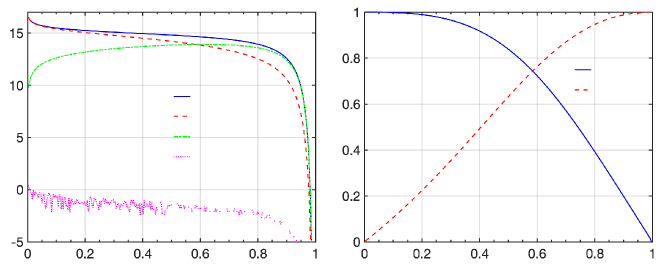
Figure 1: (a) The radiation probability log${}_{10}dW$ vs emitted photon energy $\delta_{e}=\omega_{\gamma}/\varepsilon_{i}$ for different final spins $\zeta_{f}\in\{\uparrow,\downarrow\}$ and photon polarizations $\epsilon\in\{\epsilon_{+},\epsilon_{-}\}$, where $\epsilon_{\pm}=\frac{1}{\sqrt{2}}(\mathbf{e}_{1}\pm i\mathbf{e}_{2})$. (b) The longitudinal polarization of electrons $\zeta_{f}=\frac{dW_{\uparrow}-dW_{\downarrow}}{dW_{\uparrow}+dW_{\downarrow}}$ (blue solid) and circular polarization of photons $\xi_{2}=\frac{dW_{\epsilon_{+}}-dW_{\epsilon_{-}}}{dW_{\epsilon_{+}}+dW_{\epsilon_{-}}}$ (red dashed) vs $\delta_{e}$; $\chi_{e}=1.0$, $\zeta_{i}=(0,0,1)$.

The polarization of the emitted photon resulting from the scattering process itself takes the form $\xi_{1}^{f}=\widetilde{F}_{1}/\widetilde{F}_{0}$, $\xi_{2}^{f}=\widetilde{F}_{2}/\widetilde{F}_{0}$ and $\xi_{3}^{f}=\widetilde{F}_{3}/\widetilde{F}_{0}$. In linear Compton scattering the polarization of photons is determined by the driving laser polarization, such that circularly polarized $\gamma$ photons can be obtained by linear Compton scattering of unpolarized electrons and a circularly polarized laser field. Otherwise in the nonlinear regime, see Eq.(17), the circular polarization of emitted photons is solely determined by the longitudinal polarization of initial electrons $\xi_{2}\sim\bm{\zeta}_{i}\cdot\mathbf{e}_{v}$. Thus, circularly polarized $\gamma$-photons can be generated with nonlinear Compton scattering only if electrons are initially longitudinally polarized. As an example we calculate the emission probabilities for an initially polarized electron, see Fig. 1. When the electron emits a low energy photon, the probabilities $dW_{\uparrow,\epsilon_{+}}$ and $dW_{\uparrow,\epsilon_{-}}$ dominate, leading to a small circular polarization of emitted photons. In the high energy region, $dW_{\uparrow,\epsilon_{+}}$ and $dW_{\downarrow,\epsilon_{+}}$ play leading roles, generating highly polarized gamma photons. In particular, when the emitted photon takes away nearly all the energy of the initial electron $\delta_{e}\sim 1$, $\xi_{2}\rightarrow 1$, i.e., the helicity of the electron is transferred to the emitted photon.

After averaging over initial electron polarizations, Eq.(17) becomes

$$\overline{F}_{0} =C_{0}d\omega\left\{\frac{\varepsilon^{2}+\varepsilon^{\prime 2}}{\varepsilon^{\prime}\varepsilon}\textrm{K}_{\frac{2}{3}}\left(z_{q}\right)-\int_{z_{q}}^{\infty}dx\textrm{K}_{\frac{1}{3}}\left(x\right)\right\},$$

$$\overline{F}_{1} =0,\quad\overline{F}_{2}=0,\quad\overline{F}_{3}=C_{0}d\omega\textrm{K}_{\frac{2}{3}}\left(z_{q}\right),$$ (18)

which indicates that the emitted photon is always linearly polarized when electrons spin is unresolved.

III Spin and polarization resolved pair production probability

We start from the general form of pair production probability given in Ref. [29]:

$$dW_{p} = \frac{dw_{p}}{dt}=\frac{\alpha}{\left(2\pi\right)^{2}}\frac{d^{3}p_{-}}{\omega}\int d\tau R_{p}^{*}\left(t-\frac{\tau}{2}\right)R_{p}\left(t+\frac{\tau}{2}\right)$$ (19)

$$\times \exp\left\{i\frac{\varepsilon}{\varepsilon_{f}}\left[kx\left(t+\frac{\tau}{2}\right)-kx\left(t-\frac{\tau}{2}\right)\right]\right\},$$

where $k^{\mu}=\omega\left(1,\mathbf{n}\right)$ and $x^{\mu}=\left(t,\mathbf{r}\left(t\right)\right)$ are four momentum and coordinate of the incoming photon, respectively, $\mathbf{n}$ is the unit vector in the photon propagation direction, which can be written as $\mathbf{n}=\cos\psi\cos\beta\hat{\bm{\upsilon}}+\sin\psi\cos\beta\mathbf{s}+\sin\beta\mathbf{b}$ in the angle reference system $\left(\hat{\bm{\upsilon}},\mathbf{s},\mathbf{b}\right)$. Here, $\hat{\bm{\upsilon}}$ is the unit vector along velocity of produced particles, $\mathbf{s}$ the unit vector along transverse component of acceleration $\mathbf{w}$, and $\mathbf{b}=\mathbf{\hat{\bm{\upsilon}}}\times\mathbf{s}$. For ultrarelativistic particles, the angle between vector $\mathbf{n}$ and $\bm{\upsilon}$ is of the order $1/\gamma$, therefore $\psi,\beta\sim 1/\gamma$. $\varepsilon_{+}$ and $\varepsilon_{-}$ are the energy of the created positron and electron, respectively. The integration is performed over the electron momentum $\mathbf{p}_{-}=\gamma m\bm{\upsilon}$. The expression of $R_{p}\left(t\right)$ is represented with the form

$$R_{p}\left(t\right)=i\varphi_{s}^{+}\left(\bm{\zeta}(t)\right)\left(A\left(t\right)-i\bm{\sigma}\cdot\mathbf{B}\left(t\right)\right)\varphi_{\bar{s}}\left(\bm{\zeta}^{\prime}\left(t\right)\right),$$ (20)

$\varphi_{s}\left(\bm{\zeta}\right)$ and $\varphi_{\bar{s}}\left(\bm{\zeta}^{\prime}\right)$ are the two-component spinors describing polarizations for particle and antiparticle, with $\bm{\zeta}\left(\bm{\zeta}=\bm{\zeta}_{-}\right)$ and $\mathbf{\zeta}^{\prime}\left(\mathbf{\zeta}^{\prime}=-\bm{\zeta}_{+}\right)$ being the corresponding polarization vectors. With Eq.(20), we obtain

$$R_{p}(t_{2})R_{p}^{*}(t_{1}) =\frac{1}{2}\left[A_{1}^{*}A_{2}(1-\bm{\zeta}_{-}\cdot\bm{\zeta}_{+})+\mathbf{B_{1}^{*}}\mathbf{B}_{2}(1+\bm{\zeta}_{-}\cdot\bm{\zeta}_{+})\right.$$

$$+(\bm{\zeta}_{-}\times\bm{\zeta}_{+})\cdot\left(\mathbf{B}_{1}^{*}A_{2}+\mathbf{B}_{2}A_{1}^{*}\right)$$

$$-(\bm{\zeta}_{-}\cdot\mathbf{B_{1}^{*}})(\bm{\zeta}_{+}\cdot\mathbf{B}_{2})-(\bm{\zeta}_{+}\cdot\mathbf{B_{1}^{*}})(\bm{\zeta}_{-}\cdot\mathbf{B}_{2})$$

$$+i(\bm{\zeta}_{-}-\bm{\zeta}_{+})\cdot\left(\mathbf{B_{1}^{*}}A_{2}-\mathbf{B}_{2}A_{1}^{*}\right)$$

$$\left.-i(\bm{\zeta}_{+}+\bm{\zeta}_{-})\cdot(\mathbf{B_{1}^{*}}\times\mathbf{B}_{2})\right].$$ (21)

where

$$A=N\mathbf{e}\cdot\left(\mathbf{k}\times\mathbf{p}\left(t\right)\right),$$

$$\mathbf{B}\left(t\right)=N\left\{\mathbf{e}\left[\left(\varepsilon^{\prime}+m\right)\left(\varepsilon+m\right)-\mathbf{p}^{\prime}\left(t\right)\cdot\mathbf{p}\left(t\right)\right]\right.$$

$$\quad\quad\quad\left.+\left(\mathbf{e}\cdot\mathbf{p}\left(t\right)\right)\left(\mathbf{p}^{\prime}\left(t\right)-\mathbf{p}\left(t\right)\right)\right\},$$

$$N=\left[4\varepsilon\varepsilon^{\prime}\left(\varepsilon+m\right)\left(\varepsilon^{\prime}+m\right)\right]^{-1/2},$$

with $\mathbf{e}$ being the photon polarization vector.

From now on we shall investigate pair production in a strong laser field ($a_{0}\gg 1$), where the LCFA is valid. In this case, the field inhomogeneity can be neglected when calculating the pair production rate at time $t$. Using LCFA, the terms of $\bm{\upsilon}\left(t\pm\frac{\tau}{2}\right)$ and $\mathbf{r}\left(t\pm\frac{\tau}{2}\right)$ entering the pair production probability can be expanded as Eq. (II). Repeating the same steps for calculating the radiation probability, the pair production probability can be obtained with an accuracy of $\sim 1/\gamma$. Specifically, projecting the photon polarization on the unit vectors $\bm{e}_{1}=\left(\bm{n}\times\bm{H}+\bm{E}_{\perp}\right)/\left(|\bm{n}\times\bm{H}+\bm{E}_{\perp}|\right)$ and $\bm{e}_{2}=\bm{n}\times\bm{e}_{1}$, substituting Eq. (III) into the pair production probability Eq. (19), converting to angles $\psi$ and $\beta$ with Eq. (II) and integrating over $\tau$ and the solid angle, see Appendix A, one can obtain the electron spin and photon polarization resolved pair production probability for a photon with energy $\omega$ and Stokes parameters $\xi_{i}(i=1,2,3)$ :

$$dW_{p} =\frac{1}{2}\left(dW_{11}+dW_{22}\right)+\frac{\xi_{1}}{2}\left(dW_{11}-dW_{22}\right)$$

$$-i\frac{\xi_{2}}{2}\left(dW_{21}-dW_{12}\right)+\frac{\xi_{3}}{2}\left(dW_{11}-dW_{22}\right)$$

$$=\frac{1}{2}\left(G_{0}+\xi_{1}G_{1}+\xi_{2}G_{2}+\xi_{3}G_{3}\right),$$ (22)

where

$$G_{0} =\frac{\overline{C}_{0}}{2}d\varepsilon\Bigg{\{}\left\{\int_{z_{p}}^{\infty}dx\textrm{K}_{\frac{1}{3}}\left(x\right)+\frac{\varepsilon_{+}^{2}+\varepsilon^{2}}{\varepsilon_{+}\varepsilon}\textrm{K}_{\frac{2}{3}}\left(z_{p}\right)\right\}$$

$$+\left\{\int_{z_{p}}^{\infty}dx\textrm{K}_{\frac{1}{3}}\left(x\right)-2\textrm{K}_{\frac{2}{3}}\left(z_{p}\right)\right\}\left(\bm{\zeta}_{-}\cdot\bm{\zeta}_{+}\right)$$

$$+\left[\frac{\omega}{\varepsilon_{+}}\left(\bm{\zeta}_{+}\cdot\mathbf{b}\right)-\frac{\omega}{\varepsilon}\left(\bm{\zeta}_{-}\cdot\mathbf{b}\right)\right]\textrm{K}_{\frac{1}{3}}\left(z_{p}\right)$$

$$+\left\{\frac{\varepsilon_{+}^{2}+\varepsilon^{2}}{\varepsilon\varepsilon_{+}}\int_{z_{p}}^{\infty}dx\textrm{K}_{\frac{1}{3}}\left(x\right)-\frac{\left(\varepsilon_{+}-\varepsilon\right)^{2}}{\varepsilon\varepsilon_{+}}\textrm{K}_{\frac{2}{3}}\left(z_{p}\right)\right\}$$

$$\quad\left(\bm{\zeta}_{-}\cdot\hat{\bm{\upsilon}}\right)\left(\bm{\zeta}_{+}\cdot\hat{\bm{\upsilon}}\right)\Bigg{\}}$$

$$G_{3} =\frac{\overline{C}_{0}}{2}d\varepsilon\Bigg{\{}-\textrm{K}_{\frac{2}{3}}\left(z_{p}\right)+\frac{\varepsilon_{+}^{2}+\varepsilon^{2}}{2\varepsilon_{+}\varepsilon}\textrm{K}_{\frac{2}{3}}\left(z_{p}\right)\left(\bm{\zeta}_{-}\cdot\bm{\zeta}_{+}\right)$$

$$+\left[-\frac{\omega}{\varepsilon}\left(\bm{\zeta}_{+}\cdot\mathbf{b}\right)+\frac{\omega}{\varepsilon_{+}}\left(\bm{\zeta}_{-}\cdot\mathbf{b}\right)\right]\textrm{K}_{\frac{1}{3}}\left(z_{p}\right)$$

$$-\frac{\left(\varepsilon_{+}-\varepsilon\right)^{2}}{2\varepsilon_{+}\varepsilon}\textrm{K}_{\frac{2}{3}}\left(z_{p}\right)\left(\bm{\zeta}_{-}\cdot\hat{\bm{\upsilon}}\right)\left(\bm{\zeta}_{+}\cdot\hat{\bm{\upsilon}}\right)$$

$$+\frac{\omega^{2}}{2\varepsilon_{+}\varepsilon}\int_{z_{p}}^{\infty}dx\textrm{K}_{\frac{1}{3}}\left(x\right)\left[\left(\bm{\zeta}_{-}\cdot\mathbf{b}\right)\left(\bm{\zeta}_{+}\cdot\mathbf{b}\right)-\left(\bm{\zeta}_{-}\cdot\mathbf{s}\right)\left(\bm{\zeta}_{+}\cdot\mathbf{s}\right)\right]\Bigg{\}}$$

$$G_{1} =\frac{\overline{C}_{0}}{2}d\varepsilon\Bigg{\{}-\frac{\varepsilon_{+}^{2}-\varepsilon^{2}}{2\varepsilon_{+}\varepsilon}\textrm{K}_{\frac{2}{3}}\left(z_{p}\right)\hat{\bm{\upsilon}}\cdot(\bm{\zeta}_{+}\times\bm{\zeta}_{-})$$

$$+\left[\frac{\omega}{\varepsilon}\left(\bm{\zeta}_{+}\cdot\mathbf{s}\right)-\frac{\omega}{\varepsilon_{+}}\left(\bm{\zeta}_{-}\cdot\mathbf{s}\right)\right]\textrm{K}_{\frac{1}{3}}\left(z_{p}\right)$$

$$-\frac{\omega^{2}}{2\varepsilon_{+}\varepsilon}\int_{z_{p}}^{\infty}dx\textrm{K}_{\frac{1}{3}}\left(x\right)\left\{\left(\bm{\zeta}_{-}\cdot\mathbf{b}\right)\left(\bm{\zeta}_{+}\cdot\mathbf{s}\right)+\left(\bm{\zeta}_{-}\cdot\mathbf{s}\right)\left(\bm{\zeta}_{+}\cdot\mathbf{b}\right)\right\}\Bigg{\}}$$

$$G_{2} =\frac{\overline{C}_{0}}{2}d\varepsilon\Bigg{\{}-\frac{\omega^{2}}{2\varepsilon_{+}\varepsilon}\textrm{K}_{\frac{1}{3}}\left(z_{p}\right)\left[\mathbf{s}\cdot(\bm{\zeta}_{-}\times\bm{\zeta}_{+})\right]$$

$$+\left(\frac{\omega}{\varepsilon_{+}}\int_{z_{p}}^{\infty}dx\textrm{K}_{\frac{1}{3}}\left(x\right)+\frac{\varepsilon_{+}^{2}-\varepsilon^{2}}{\varepsilon_{+}\varepsilon}\textrm{K}_{\frac{2}{3}}\left(z_{p}\right)\right)\left(\bm{\zeta}_{+}\cdot\hat{\bm{\upsilon}}\right)$$

$$+\left(\frac{\omega}{\varepsilon}\int_{z_{p}}^{\infty}dx\textrm{K}_{\frac{1}{3}}\left(x\right)-\frac{\varepsilon_{+}^{2}-\varepsilon^{2}}{\varepsilon_{+}\varepsilon}\textrm{K}_{\frac{2}{3}}\left(z_{p}\right)\right)\left(\bm{\zeta}_{-}\cdot\hat{\bm{\upsilon}}\right)$$

$$-\frac{\varepsilon_{+}^{2}-\varepsilon^{2}}{2\varepsilon_{+}\varepsilon}\textrm{K}_{\frac{1}{3}}\left(z_{p}\right)\left[\left(\bm{\zeta}_{-}\cdot\hat{\bm{\upsilon}}\right)\left(\bm{\zeta}_{+}\cdot\mathbf{b}\right)+\left(\bm{\zeta}_{-}\cdot\mathbf{b}\right)\left(\bm{\zeta}_{+}\cdot\hat{\bm{\upsilon}}\right)\right]\Bigg{\}}.$$ (23)

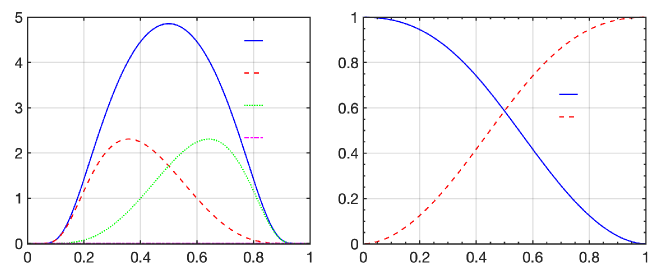
Figure 2: (a) The pair production probability $dW_{\zeta_{-}\zeta_{+}}$ vs relative energy of electron $\delta_{-}=\varepsilon/\omega$ for different final spins of electron $\zeta^{f}_{-}\in\{\uparrow,\downarrow\}$ and positron $\zeta^{f}_{+}\in\{\uparrow,\downarrow\}$. (b) The longitudinal polarization of electrons $\zeta^{f}_{-}=\frac{\sum_{i}dW_{\uparrow,i}-\sum_{i}dW_{\downarrow,i}}{\sum_{i}dW_{\uparrow,i}+\sum_{i}dW_{\downarrow,i}}$ (blue solid) and positrons $\zeta^{f}_{+}=\frac{\sum_{i}dW_{i,\uparrow}-\sum_{i}dW_{i,\downarrow}}{\sum_{i}dW_{i,\uparrow}+\sum_{i}dW_{i,\downarrow}}$ (red dashed) vs $\delta_{-}$; $\chi_{\gamma}=1.0$, $\xi=(0,1,0)$.

Here $\overline{C}_{0}=\frac{\alpha m^{2}d\varepsilon}{\sqrt{3}\pi\omega^{2}}$ and $z_{p}=\frac{2}{3\chi_{\gamma}}\frac{\omega^{2}}{\varepsilon_{+}\varepsilon_{-}}$. After taking the sum over positron polarizations, we arrive at the results given in Ref. [29]:

$$\widetilde{G}_{0} =\overline{C}_{0}d\varepsilon\Bigg{\{}\int_{z_{p}}^{\infty}dx\textrm{K}_{\frac{1}{3}}\left(x\right)+\frac{\varepsilon_{+}^{2}+\varepsilon^{2}}{\varepsilon_{+}\varepsilon}\textrm{K}_{\frac{2}{3}}\left(z_{p}\right)-\frac{\omega}{\varepsilon}\left(\bm{\zeta}_{-}\cdot\mathbf{b}\right)\textrm{K}_{\frac{1}{3}}\left(z_{p}\right)\Bigg{\}}$$

$$\widetilde{G}_{3} =\overline{C}_{0}d\varepsilon\Bigg{\{}-\textrm{K}_{\frac{2}{3}}\left(z_{p}\right)+\frac{\omega}{\varepsilon_{+}}\left(\bm{\zeta}_{-}\cdot\mathbf{b}\right)\textrm{K}_{\frac{1}{3}}\left(z_{p}\right)\Bigg{\}}$$

$$\widetilde{G}_{1} =-\overline{C}_{0}d\varepsilon\frac{\omega}{\varepsilon_{+}}\left(\bm{\zeta}_{-}\cdot\mathbf{s}\right)\textrm{K}_{\frac{1}{3}}\left(z_{p}\right)$$

$$\widetilde{G}_{2} =\overline{C}_{0}d\varepsilon\Bigg{\{}\left(\frac{\omega}{\varepsilon}\int_{z_{p}}^{\infty}dx\textrm{K}_{\frac{1}{3}}\left(x\right)-\frac{\varepsilon_{+}^{2}-\varepsilon^{2}}{\varepsilon_{+}\varepsilon}\textrm{K}_{\frac{2}{3}}\left(z_{p}\right)\right)\left(\bm{\zeta}_{-}\cdot\hat{\bm{\upsilon}}\right)\Bigg{\}}.$$

The polarization of the final electron can be expressed as

$$\bm{\zeta}_{-}^{f}=-\frac{\xi_{1}\textrm{K}_{\frac{1}{3}}\left(z_{p}\right)\frac{\omega}{\varepsilon_{+}}\mathbf{s}+\xi_{2}\hat{\bm{\upsilon}}\left(-\frac{\omega}{\varepsilon}\int_{z_{p}}^{\infty}dx\textrm{K}_{\frac{1}{3}}\left(x\right)+\frac{\varepsilon_{+}^{2}-\varepsilon^{2}}{\varepsilon\varepsilon_{+}}\textrm{K}_{\frac{2}{3}}\left(z_{p}\right)\right)+\left(\frac{\omega}{\varepsilon}-\xi_{3}\frac{\omega}{\varepsilon_{+}}\right)\mathbf{b}\textrm{K}_{\frac{1}{3}}\left(z_{p}\right)}{\int_{z_{p}}^{\infty}dx\textrm{K}_{\frac{1}{3}}\left(x\right)+\frac{\varepsilon^{2}+\varepsilon_{+}^{2}}{\varepsilon\varepsilon_{+}}\textrm{K}_{\frac{2}{3}}\left(z_{p}\right)-\xi_{3}\textrm{K}_{\frac{2}{3}}\left(z_{p}\right)}.$$ (24)

In nonlinear Breit-Wheeler process, see Eq.(24), the longitudinal polarization of the created electrons is solely determined by circular polarization of initial gamma photons $\zeta_{\parallel}\equiv\bm{\zeta}_{-}\cdot\mathbf{e}_{v}\propto\xi_{2}$. Thus, longitudinal polarized electrons can be generated via the nonlinear Breit-Wheeler process only if initial gamma photons are circularly polarized. As an example we calculate the pair production probabilities for an circularly polarized gamma photon, see Fig. 2. When a low energy electron is created, the probabilities $dW_{\uparrow\uparrow}$ and $dW_{\downarrow\uparrow}$ dominate, leading to a small longitudinal polarization of created electrons. In the high energy region, $dW_{\uparrow\uparrow}$ and $dW_{\uparrow\downarrow}$ play leading roles, generating highly longitudinally polarized electron. In particular, $\bm{\zeta}_{-}^{f}=\xi_{2}\mathbf{e}_{v}$ when $\varepsilon\approx\omega$. This is the case when helicity transfer occurs. For this reason, it is possible to produce longitudinally polarized positrons via the Breit-Wheeler process [78]. After taking the sum over positron and electron polarizations, we get the spin unresolved pair production probability:

$$\overline{G}_{0} =2\overline{C}_{0}d\varepsilon\Bigg{\{}\int_{z_{p}}^{\infty}dx\textrm{K}_{\frac{1}{3}}\left(x\right)+\frac{\varepsilon_{+}^{2}+\varepsilon^{2}}{\varepsilon_{+}\varepsilon}\textrm{K}_{\frac{2}{3}}\left(z_{p}\right)\Bigg{\}},$$

$$\overline{G}_{3}=-2\overline{C}_{0}d\varepsilon\textrm{K}_{\frac{2}{3}}\left(z_{p}\right),\overline{G}_{1}=0,\overline{G}_{2}=0.$$ (25)

As expected, the dependence on circular polarization of the photon is vanishing if the spin is unresolved.

IV Conclusion

Some of the results are already applied to the simulation codes in our previous works but without derivation [75, 76, 79, 78, 80, 77]. In this paper, we give a rigorous derivation of the electron spin and photon polarization fully resolved radiation and pair production probabilities. Using Baier-Katkov semiclassical method, we obtain the complete set of the radiation and pair production probabilities for arbitrary initial and final electron-positron spins and arbitrary polarization of the incoming and outgoing photons within the LCFA and quasiclasscial approximation. The fully polarization-resolved probabilities are written in a compact form, and are applicable for arbitrary pulse shapes and polarization as long as $a_{0}\gg 1$ and $\gamma\gg 1$. Therefore, the formulas can be easily implemented into QED Monte Carlo simulation codes for investigating polarization effects during nonlinear Compton scattering and Breit-Wheeler processes, and are essential for polarization effect studies in strong field QED precesses.

Appendix A Calculation of the integrals

The integration over $\tau$ in Eq. (11) employs the following results:

$$\int_{-\infty}^{\infty}dx\cos\left(bx+ax^{3}\right) =\frac{2}{3}\sqrt{\frac{b}{a}}\textrm{K}_{\frac{1}{3}}\left(\frac{2}{3\sqrt{3}}\frac{b^{\frac{3}{2}}}{\sqrt{a}}\right),$$

$$\int_{-\infty}^{\infty}dx\,x\,\sin\left(bx+ax^{3}\right) =\frac{2}{3\sqrt{3}}\frac{b}{a}\textrm{K}_{\frac{2}{3}}\left(\frac{2}{3\sqrt{3}}\frac{b^{\frac{3}{2}}}{\sqrt{a}}\right),$$

$$\int_{-\infty}^{\infty}dx\,x^{2}\cos\left(bx+ax^{3}\right) =-\frac{2}{9}\left(\frac{b}{a}\right)^{\frac{3}{2}}\textrm{K}_{\frac{1}{3}}\left(\frac{2}{3\sqrt{3}}\frac{b^{\frac{3}{2}}}{\sqrt{a}}\right).$$ (26)

Therefore, we have

$$I_{0} =\int_{-\infty}^{\infty}d\tau\exp\left\{-i\frac{\varepsilon\omega}{\varepsilon_{f}}\left[\left(1-\mathbf{n}\mathbf{v}\right)\tau+\frac{\tau^{3}}{24}\mathbf{w}^{2}\right]\right\}$$

$$=\frac{2\sqrt{24}}{3w}\sqrt{\left(1-\mathbf{n}\mathbf{v}\right)}\textrm{K}_{\frac{1}{3}}\left(\xi\right),$$

$$I_{1}=\int_{-\infty}^{\infty}d\tau\tau\exp\left\{-i\frac{\varepsilon\omega}{\varepsilon_{f}}\left[\left(1-\mathbf{n}\mathbf{v}\right)\tau+\frac{\tau^{3}}{24}\mathbf{w}^{2}\right]\right\}$$

$$=-i\frac{16}{\sqrt{3}}\frac{1}{w^{2}}\left(1-\mathbf{n}\mathbf{v}\right)\textrm{K}_{\frac{2}{3}}\left(\xi\right),$$

$$I_{2}=\int_{-\infty}^{\infty}d\tau\tau^{2}\exp\left\{-i\frac{\varepsilon\omega}{\varepsilon_{f}}\left[\left(1-\mathbf{n}\mathbf{v}\right)\tau+\frac{\tau^{3}}{24}\mathbf{w}^{2}\right]\right\}$$

$$=-\frac{2\left(24\right)^{\frac{3}{2}}}{9w^{3}}\left(1-\mathbf{n}\mathbf{v}\right)^{\frac{3}{2}}\textrm{K}_{\frac{1}{3}}\left(\xi\right).$$ (27)

Integrating Eq.(14) over solid angles, one obtains the integrals for deriving the radiation probability:

$$\int d\Omega I_{0} =\frac{4\sqrt{3}}{3}\pi\frac{\varepsilon^{\prime}}{\varepsilon\omega}\int_{z_{q}}^{\infty}dx\textrm{K}_{\frac{1}{3}}\left(x\right),$$

$$\int d\Omega I_{1} =-i\frac{8}{\sqrt{3}}\frac{1}{w}\pi\frac{1}{\gamma}\frac{\varepsilon^{\prime}}{\varepsilon\omega}\textrm{K}_{\frac{1}{3}}\left(z_{q}\right),$$

$$\int d\Omega I_{2} =-\frac{16}{\sqrt{3}w^{2}}\pi\frac{1}{\gamma^{2}}\frac{\varepsilon^{\prime}}{\varepsilon\omega}\textrm{K}_{\frac{2}{3}}\left(z_{q}\right).$$ (28)

Similarly, the pair production probability can be obtained with the integration over $\tau$:

$$I_{0} =\int_{-\infty}^{\infty}d\tau\exp\left\{i\frac{\varepsilon\omega}{\varepsilon_{+}}\left[\left(1-\mathbf{n}\mathbf{v}\right)\tau+\frac{\tau^{3}}{24}\mathbf{w}^{2}\right]\right\}$$

$$=\frac{2\sqrt{24}}{3w}\sqrt{\left(1-\mathbf{n}\mathbf{v}\right)}\textrm{K}_{\frac{1}{3}}\left(\xi\right),$$

$$I_{1}=\int_{-\infty}^{\infty}d\tau\tau\exp\left\{i\frac{\varepsilon\omega}{\varepsilon_{+}}\left[\left(1-\mathbf{n}\mathbf{v}\right)\tau+\frac{\tau^{3}}{24}\mathbf{w}^{2}\right]\right\}$$

$$=i\frac{16}{\sqrt{3}}\frac{1}{w^{2}}\left(1-\mathbf{n}\mathbf{v}\right)\textrm{K}_{\frac{2}{3}}\left(\xi\right),$$

$$I_{2}=\int_{-\infty}^{\infty}d\tau\tau^{2}\exp\left\{i\frac{\varepsilon\omega}{\varepsilon_{+}}\left[\left(1-\mathbf{n}\mathbf{v}\right)\tau+\frac{\tau^{3}}{24}\mathbf{w}^{2}\right]\right\}$$

$$=-\frac{2\left(24\right)^{\frac{3}{2}}}{9w^{3}}\left(1-\mathbf{n}\mathbf{v}\right)^{\frac{3}{2}}\textrm{K}_{\frac{1}{3}}\left(\xi\right).$$ (29)

and the solid angle integrations give

$$\int d\Omega I_{0} =\frac{4\sqrt{3}}{3}\pi\frac{\varepsilon_{+}}{\varepsilon\omega}\int_{z_{p}}^{\infty}dx\textrm{K}_{\frac{1}{3}}\left(x\right),$$

$$\int d\Omega I_{1} =i\frac{8}{\sqrt{3}}\frac{1}{w}\pi\frac{1}{\gamma}\frac{\varepsilon_{+}}{\varepsilon\omega}\textrm{K}_{\frac{1}{3}}\left(z_{p}\right),$$

$$\int d\Omega I_{2} =-\frac{16}{\sqrt{3}w^{2}}\pi\frac{1}{\gamma^{2}}\frac{\varepsilon_{+}}{\varepsilon\omega}\textrm{K}_{\frac{2}{3}}\left(z_{p}\right).$$

References

• Anthony et al. [2004] P. Anthony, R. Arnold, C. Arroyo, K. Baird, K. Bega, J. Biesiada, P. Bosted, M. Breuer, R. Carr, G. Cates, et al., Observation of parity nonconservation in møller scattering, Physical review letters 92, 181602 (2004).
• Moortgat-Pick et al. [2008] G. Moortgat-Pick, T. Abe, G. Alexander, B. Ananthanarayan, A. Babich, V. Bharadwaj, D. Barber, A. Bartl, A. Brachmann, S. Chen, et al., Polarized positrons and electrons at the linear collider, Physics Reports 460, 131 (2008).
• Horikawa et al. [2014] K. Horikawa, S. Miyamoto, T. Mochizuki, S. Amano, D. Li, K. Imasaki, Y. Izawa, K. Ogata, S. Chiba, and T. Hayakawa, Neutron angular distribution in ($\gamma$, n) reactions with linearly polarized $\gamma$-ray beam generated by laser compton scattering, Physics Letters B 737, 109 (2014).
• Uggerhøj [2005] U. I. Uggerhøj, The interaction of relativistic particles with strong crystalline fields, Reviews of modern physics 77, 1131 (2005).
• Abe et al. [1995] K. Abe, T. Akagi, P. Anthony, R. Antonov, R. Arnold, T. Averett, H. Band, J. Bauer, H. Borel, P. Bosted, et al., Precision measurement of the deuteron spin structure function g 1 d, Physical Review Letters 75, 25 (1995).
• Alexakhin et al. [2007] V. Y. Alexakhin, Y. Alexandrov, G. Alexeev, M. Alexeev, A. Amoroso, B. Badełek, F. Balestra, J. Ball, J. Barth, G. Baum, et al., The deuteron spin-dependent structure function g1d and its first moment, Physics Letters B 647, 8 (2007).
• Kessler [2013] J. Kessler, Polarized electrons, Vol. 1 (Springer Science & Business Media, 2013).
• Getzlaff [2010] M. Getzlaff, Experimental aspects, in Surface Magnetism (Springer, 2010) pp. 5–20.
• Borisov and Grishina [1996] A. Borisov and V. Y. Grishina, Compton production of axions on electrons in a constant external field, Journal of Experimental and Theoretical Physics 83, 868 (1996).
• Herczeg [2003] P. Herczeg, Cp-violating electron-nucleon interactions from leptoquark exchange, Physical Review D 68, 116004 (2003).
• Ananthanarayan and Rindani [2018] B. Ananthanarayan and S. D. Rindani, Inclusive spin–momentum analysis and new physics at a polarized electron–positron collider, The European Physical Journal C 78, 1 (2018).
• Godbole et al. [2006] R. M. Godbole, S. D. Rindani, and R. K. Singh, Lepton distribution as a probe of new physics in production and decay of the t quark and its polarization, Journal of High Energy Physics 2006, 021 (2006).
• Akbar et al. [2017] Z. Akbar, P. Roy, S. Park, V. Crede, A. Anisovich, I. Denisenko, E. Klempt, V. Nikonov, A. Sarantsev, K. Adhikari, et al., Measurement of the helicity asymmetry e in $\omega\rightarrow\pi$+ $\pi$- $\pi$ 0 photoproduction, Physical Review C 96, 065209 (2017).
• Nakamiya and Homma [2017] Y. Nakamiya and K. Homma, Probing vacuum birefringence under a high-intensity laser field with gamma-ray polarimetry at the gev scale, Physical Review D 96, 053002 (2017).
• Bragin et al. [2017] S. Bragin, S. Meuren, C. H. Keitel, and A. Di Piazza, High-energy vacuum birefringence and dichroism in an ultrastrong laser field, Physical review letters 119, 250403 (2017).
• King and Elkina [2016] B. King and N. Elkina, Vacuum birefringence in high-energy laser-electron collisions, Physical Review A 94, 062102 (2016).
• Ilderton and Marklund [2016] A. Ilderton and M. Marklund, Prospects for studying vacuum polarisation using dipole and synchrotron radiation, Journal of Plasma Physics 82 (2016).
• Ataman et al. [2017] S. Ataman, M. Cuciuc, L. D’Alessi, L. Neagu, M. Rosu, K. Seto, O. Tesileanu, Y. Xu, and M. Zeng, Experiments with combined laser and gamma beams at eli-np, in AIP Conference Proceedings, Vol. 1852 (AIP Publishing LLC, 2017) p. 070002.
• Hu et al. [2010] H. Hu, C. Müller, and C. H. Keitel, Complete qed theory of multiphoton trident pair production in strong laser fields, Physical review letters 105, 080401 (2010).
• Ilderton [2011] A. Ilderton, Trident pair production in strong laser pulses, Physical review letters 106, 020404 (2011).
• King and Ruhl [2013] B. King and H. Ruhl, Trident pair production in a constant crossed field, Physical Review D 88, 013005 (2013).
• Morozov and Ritus [1975] D. Morozov and V. Ritus, Elastic electron scattering in an intense field and two-photon emission, Nuclear Physics B 86, 309 (1975).
• Seipt and Kämpfer [2012] D. Seipt and B. Kämpfer, Two-photon compton process in pulsed intense laser fields, Physical Review D 85, 101701 (2012).
• Mackenroth and Di Piazza [2013] F. Mackenroth and A. Di Piazza, Nonlinear double compton scattering in the ultrarelativistic quantum regime, Physical review letters 110, 070402 (2013).
• King [2015] B. King, Double compton scattering in a constant crossed field, Physical Review A 91, 033415 (2015).
• Seipt et al. [2021] D. Seipt, C. P. Ridgers, D. Del Sorbo, and A. G. Thomas, Polarized qed cascades, New Journal of Physics 23, 053025 (2021).
• Nerush et al. [2011] E. Nerush, I. Y. Kostyukov, A. Fedotov, N. Narozhny, N. Elkina, and H. Ruhl, Laser field absorption in self-generated electron-positron pair plasma, Physical review letters 106, 035001 (2011).
• Ritus [1985] V. I. Ritus, J. Sov. Laser Res. 6, 497 (1985).
• Baier et al. [1998] V. N. Baier, V. M. Katkov, and V. M. Strakhovenko, Electromagnetic Processes at High Energies in Oriented Single Crystals (World Scientific, Singapore, 1998).
• Seipt and Kämpfer [2011] D. Seipt and B. Kämpfer, Nonlinear compton scattering of ultrashort intense laser pulses, Physical Review A 83, 022101 (2011).
• Heinzl et al. [2010] T. Heinzl, D. Seipt, and B. Kämpfer, Beam-shape effects in nonlinear compton and thomson scattering, Physical Review A 81, 022125 (2010).
• Bocquet et al. [1997] J. Bocquet, J. Ajaka, M. Anghinolfi, V. Bellini, G. Berrier, P. Calvat, M. Capogni, L. Casano, M. Castoldi, P. Corvisiero, et al., Graal: a polarized $\gamma$-ray beam at esrf, Nuclear Physics A 622, c124 (1997).
• Yoon et al. [2021] J. W. Yoon, Y. G. Kim, I. W. Choi, J. H. Sung, H. W. Lee, S. K. Lee, and C. H. Nam, Realization of laser intensity over 1023 w/cm2, Optica 8, 630 (2021).
• Burdonov et al. [2021] K. Burdonov, A. Fazzini, V. Lelasseux, J. Albrecht, P. Antici, Y. Ayoul, A. Beluze, D. Cavanna, T. Ceccotti, M. Chabanis, A. Chaleil, S. N. Chen, Z. Chen, F. Consoli, M. Cuciuc, X. Davoine, J. P. Delaneau, E. D’Humières, J.-L. Dubois, C. Evrard, E. Filippov, A. Freneaux, P. Forestier-Colleoni, L. Gremillet, V. Horny, L. Lancia, L. Lecherbourg, N. Lebas, A. Leblanc, W. Ma, L. Martin, F. Negoita, J.-L. Paillard, D. Papadopoulos, F. Perez, S. Pikuz, G. Qi, F. Quéré, L. Ranc, P. A. Söderstrom, M. Scisciò, S. Sun, S. Vallières, P. Wang, W. Yao, F. Mathieu, P. Audebert, and J. Fuchs, Characterization and performance of the Apollon Short-Focal-Area facility following its commissioning at 1 PW level, arxiv: 2108.01336  (2021).
• Laso Garcia et al. [2021] A. Laso Garcia, H. Höppner, A. Pelka, C. Bähtz, E. Brambrink, S. Di Dio Cafiso, J. Dreyer, S. Göde, M. Hassan, T. Kluge, J. Liu, M. Makita, D. Möller, M. Nakatsutsumi, T. R. Preston, G. Priebe, H. P. Schlenvoigt, J. P. Schwinkendorf, M. Šmíd, A. M. Talposi, M. Toncian, U. Zastrau, U. Schramm, T. E. Cowan, and T. Toncian, ReLaX: the Helmholtz International Beamline for Extreme Fields high-intensity short-pulse laser driver for relativistic laser–matter interaction and strong-field science using the high energy density instrument at the European X-ray free electron laser fa, High Power Laser Science and Engineering 9, 59 (2021).
• Hong et al. [2021] W. Hong, S. He, J. Teng, Z. Deng, Z. Zhang, F. Lu, B. Zhang, B. Zhu, Z. Dai, B. Cui, Y. Wu, D. Liu, W. Qi, J. Jiao, F. Zhang, Z. Yang, F. Zhang, B. Bi, X. Zeng, K. Zhou, Y. Zuo, X. Huang, N. Xie, Y. Guo, J. Su, D. Han, Y. Mao, L. Cao, W. Zhou, Y. Gu, F. Jing, B. Zhang, H. Cai, M. He, W. Zheng, S. Zhu, W. Ma, D. Wang, Y. Shou, X. Yan, B. Qiao, Y. Zhang, C. Zhong, X. Yuan, and W. Wei, Commissioning experiment of the high-contrast SILEX-II multi-petawatt laser facility, Matter and Radiation at Extremes 6, 064401 (2021).
• [37] The Vulcan facility, http://www.clf.stfc.ac.uk/Pages/TheVulcan-10-Petawatt-Project.aspx.
• [38] The Extreme Light Infrastructure (ELI), http://www.elibeams.eu/en/facility/lasers/.
• [39] Exawatt Center for Extreme Light Studies (XCELS), http://www.xcels.iapras.ru/.
• Di Piazza et al. [2012a] A. Di Piazza, C. Müller, K. Z. Hatsagortsyan, and C. H. Keitel, Extremely high-intensity laser interactions with fundamental quantum systems, Rev. Mod. Phys. 84, 1177 (2012a).
• Heinzl [2012] T. Heinzl, Strong-field qed and high-power lasers, Int. J. Mod. Phys. A 27, 1260010 (2012).
• Seipt and King [2020] D. Seipt and B. King, Spin-and polarization-dependent locally-constant-field-approximation rates for nonlinear compton and breit-wheeler processes, Physical Review A 102, 052805 (2020).
• King and Tang [2020] B. King and S. Tang, Nonlinear compton scattering of polarized photons in plane-wave backgrounds, Physical Review A 102, 022809 (2020).
• Wistisen [2014] T. N. Wistisen, Interference effect in nonlinear compton scattering, Physical Review D 90, 125008 (2014).
• Mackenroth and Di Piazza [2011] F. Mackenroth and A. Di Piazza, Nonlinear compton scattering in ultrashort laser pulses, Physical Review A 83, 032106 (2011).
• Dinu and Torgrimsson [2020] V. Dinu and G. Torgrimsson, Approximating higher-order nonlinear qed processes with first-order building blocks, Phys. Rev. D 102, 016018 (2020).
• Torgrimsson [2021] G. Torgrimsson, Loops and polarization in strong-field QED, New J. Phys. 23, 065001 (2021).
• Bagrov and Gitman [1990] V. G. Bagrov and D. M. Gitman, Exact Solutions of Relativistic Wave Equations (Kluwer Academic Publishers, Dordrecht, 1990).
• Wolkow [1935] D. M. Wolkow, Über eine Klasse von Lösungen der Diracschen Gleichung, Z. Phys. 94, 250 (1935).
• Ritus [1972a] V. Ritus, Radiative corrections in quantum electrodynamics with intense field and their analytical properties, Annals of Physics 69, 555 (1972a).
• Bol’Shedvorsky et al. [2000] E. Bol’Shedvorsky, S. Polityko, and A. Misaki, Spin of scattered electrons in the nonlinear compton effect, Progress of Theoretical Physics 104, 769 (2000).
• King et al. [2013] B. King, N. Elkina, and H. Ruhl, Photon polarization in electron-seeded pair-creation cascades, Physical Review A 87, 042117 (2013).
• Tang et al. [2020] S. Tang, B. King, and H. Hu, Highly polarised gamma photons from electron-laser collisions, Physics Letters B 809, 135701 (2020).
• Chen et al. [2018] Y.-Y. Chen, J.-X. Li, K. Z. Hatsagortsyan, and C. H. Keitel, $\gamma$-ray beams with large orbital angular momentum via nonlinear compton scattering with radiation reaction, Physical review letters 121, 074801 (2018).
• Ivanov et al. [2004] D. Y. Ivanov, G. Kotkin, and V. Serbo, Complete description of polarization effects in emission of a photon by an electron in the field of a strong laser wave, The European Physical Journal C-Particles and Fields 36, 127 (2004).
• Di Piazza et al. [2012b] A. Di Piazza, C. Müller, K. Hatsagortsyan, and C. H. Keitel, Extremely high-intensity laser interactions with fundamental quantum systems, Reviews of Modern Physics 84, 1177 (2012b).
• Seipt et al. [2018] D. Seipt, D. Del Sorbo, C. Ridgers, and A. Thomas, Theory of radiative electron polarization in strong laser fields, Physical Review A 98, 023417 (2018).
• Di Piazza et al. [2018] A. Di Piazza, M. Tamburini, S. Meuren, and C. Keitel, Implementing nonlinear compton scattering beyond the local-constant-field approximation, Physical Review A 98, 012134 (2018).
• Di Piazza et al. [2019] A. Di Piazza, M. Tamburini, S. Meuren, and C. H. Keitel, Improved local-constant-field approximation for strong-field qed codes, Physical Review A 99, 022125 (2019).
• Lv et al. [2021] Q. Lv, E. Raicher, C. Keitel, and K. Hatsagortsyan, Anomalous violation of the local constant field approximation in colliding laser beams, Physical Review Research 3, 013214 (2021).
• Dinu et al. [2016] V. Dinu, C. Harvey, A. Ilderton, M. Marklund, and G. Torgrimsson, Quantum radiation reaction: from interference to incoherence, Physical review letters 116, 044801 (2016).
• Ilderton et al. [2019] A. Ilderton, B. King, and D. Seipt, Extended locally constant field approximation for nonlinear compton scattering, Physical Review A 99, 042121 (2019).
• Bamber et al. [1999] C. Bamber, S. Boege, T. Koffas, T. Kotseroglou, A. Melissinos, D. Meyerhofer, D. Reis, W. Ragg, C. Bula, K. McDonald, et al., Studies of nonlinear qed in collisions of 46.6 gev electrons with intense laser pulses, Physical Review D 60, 092004 (1999).
• Burke et al. [1997] D. Burke, R. Field, G. Horton-Smith, J. Spencer, D. Walz, S. Berridge, W. Bugg, K. Shmakov, A. Weidemann, C. Bula, et al., Positron production in multiphoton light-by-light scattering, Physical Review Letters 79, 1626 (1997).
• Villalba-Chávez and Müller [2013] S. Villalba-Chávez and C. Müller, Photo-production of scalar particles in the field of a circularly polarized laser beam, Physics Letters B 718, 992 (2013).
• Jansen et al. [2016] M. Jansen, J. Kamiński, K. Krajewska, and C. Müller, Strong-field breit-wheeler pair production in short laser pulses: Relevance of spin effects, Physical Review D 94, 013010 (2016).
• Nikishov and Ritus [1964] A. Nikishov and V. Ritus, Zh. eksper. teor. fiz. 46, 776 (1963) english translation, Soviet Physics (SET?) 19 529 (1964).
• Nikishov and Ritus [1967] A. Nikishov and V. Ritus, Pair production by a photon and photon emission by an electron in the field of an intense electromagnetic wave and in a constant field, Sov. Phys. JETP 25, 1135 (1967).
• Ritus [1972b] V. Ritus, Vacuum polarization correction to elastic electron and muon scattering in an intense field and pair electro-and muoproduction, Nuclear Physics B 44, 236 (1972b).
• Ritus [1970] V. Ritus, Radiative effects and their enhancement in an intense electromagnetic field, Sov. Phys. JETP 30, 052805 (1970).
• Ivanov et al. [2005] D. Y. Ivanov, G. Kotkin, and V. Serbo, Complete description of polarization effects in e+ e-pair productionby a photon in the field of a strong laser wave, The European Physical Journal C-Particles and Fields 40, 27 (2005).
• Tsai [1993] Y. S. Tsai, Laser+e${}^{-}\rightarrow\gamma+e^{-}$and laser+ $\gamma\rightarrow e^{+}+e^{-}$ as sources of producing circularly polarized $\gamma$ and $e^{\pm}$ beams, Physical Review D 48, 96 (1993).
• Berestetskii et al. [1982] V. B. Berestetskii, , E. M. Lifshitz, and L. P. Pitevskii, Quantum electrodynamics (Pergamon, Oxford, 1982).
• Wistisen [2020] T. N. Wistisen, Numerical approach to the semiclassical method of pair production for arbitrary spins and photon polarization, Physical Review D 101, 076017 (2020).
• Li et al. [2019] Y.-F. Li, R. Shaisultanov, K. Z. Hatsagortsyan, F. Wan, C. H. Keitel, and J.-X. Li, Ultrarelativistic electron-beam polarization in single-shot interaction with an ultraintense laser pulse, Phys. Rev. Lett. 122, 154801 (2019).
• Chen et al. [2019] Y.-Y. Chen, P.-L. He, R. Shaisultanov, K. Z. Hatsagortsyan, and C. H. Keitel, Polarized positron beams via intense two-color laser pulses, Phys. Rev. Lett. 123, 174801 (2019).
• Wan et al. [2020] F. Wan, R. Shaisultanov, Y.-F. Li, K. Z. Hatsagortsyan, C. H. Keitel, and J.-X. Li, Ultrarelativistic polarized positron jets via collision of electron and ultraintense laser beams, Phys. Lett. B 800, 135120 (2020).
• Li et al. [2020a] Y.-F. Li, Y.-Y. Chen, W.-M. Wang, and H.-S. Hu, Production of highly polarized positron beams via helicity transfer from polarized electrons in a strong laser field, Physical Review Letters 125, 044802 (2020a).
• Li et al. [2020b] Y.-F. Li, R. Shaisultanov, Y.-Y. Chen, F. Wan, K. Z. Hatsagortsyan, C. H. Keitel, and J.-X. Li, Polarized ultrashort brilliant multi-gev $\gamma$ rays via single-shot laser-electron interaction, Phys. Rev. Lett. 124, 014801 (2020b).
• Wan et al. [2021] F. Wan, Y. Wang, R.-T. Guo, Y.-Y. Chen, R. Shaisultanov, Z.-F. Xu, K. Z. Hatsagortsyan, C. H. Keitel, and J.-X. Li, High-energy $\gamma$-photon polarization in nonlinear breit-wheeler pair production and $\gamma$-polarimetry, Fundamental Research 1 (2021).
• Baier and Katkov [1967a] V. N. Baier and V. M. Katkov, Radiative polarization of electrons in a magnetic fleld, Soviet Phys. JETP 25, 944 (1967a).
• Baier and Katkov [1967b] V. N. Baier and V. M. Katkov, Quantum effects in magnetic bremsstrahlung, Physics Letters A 25, 492 (1967b).
• Schwinger [1954] J. Schwinger, The quantum correctios in the radiation by energetic accelerated electrons, Proc. US Nat. Acad. Sci. 40, 132 (1954).