Magnetoconductance Anisotropies and Aharonov-Casher Phases

Abstract

The spin-orbit interaction (SOI) is a key tool for manipulating and functionalizing spin-dependent electron transport. The desired function often depends on the SOI-generated phase that is accumulated by the wave function of an electron as it passes through the device. This phase, known as the Aharonov-Casher phase, therefore depends on both the device geometry and the SOI strength. Here we propose a method for directly measuring the Aharonov-Casher phase generated in an SOI-active weak link, based on the Aharonov-Casher-phase dependent anisotropy of its magnetoconductance. Specifically we consider weak links in which the Rashba interaction is caused by an external electric field, but our method is expected to apply also for other forms of the spin-orbit coupling. Measuring this magnetoconductance anisotropy thus allows calibrating Rashba spintronic devices by an external electric field that tunes the spin-orbit interaction and hence the Aharonov-Casher phase.

Introduction. The spin-orbit interaction (SOI), which allows for an interplay between charge and spin currents in all-electrical devices Sahoo ; Hirohata , substantially affects the transport properties of two- and three-dimensional conductors. The spin-Hall effect Wunderlich , the electrical control of the magnetization in magnetic heterostructures by interfacial spin-orbit toques Amin , and the spin relaxation yielding quantum anti weak-localization in impure conductors Bergmann ; Iizasa are examples of such an influence.

The SOI is due to the interaction between the magnetic moment $\mu$ of a particle moving with velocity ${\bf v}$ through a static electric field E and the magnetic field B${}_{\rm so}=(\bf{E}\times\bf{v})/$c² seen in the rest frame of the particle. This relativistic effect adds a term

$${\cal H}_{\rm so}(k)={\mbox{\boldmath{$\mu$}}}\cdot{\bf B}_{\rm so}={\mbox{\boldmath{$\mu$}}}\cdot({\bf E}\times{\bf v})/c^{2}.$$ (1)

to the Hamiltonian, which can be removed by a gauge transformation, $\Psi\to\exp(i\hat{\phi}_{\rm AC})\Psi$, that adds a phase factor to the wave function. Here

$$\hat{\phi}_{\rm AC}=-\frac{1}{\hbar}\int^{t}{\mbox{\boldmath{$\mu$}}}\cdot{\bf B}_{\rm so}dt^{\prime}=\frac{1}{\hbar c^{2}}\int^{\bf r}({\bf E}\times{{\mbox{\boldmath{$\mu$}}}})\cdot d{\bf r}^{\prime},$$ (2)

where the integration is over the path of the particle, is known as the Aharonov-Casher phase AC ; Qian . We use the notation $\hat{\phi}_{\rm AC}$ for the phase operator and $\phi_{\rm AC}$ for its eigenvalue, to be discussed below.

One notes from Eqs. (1) and (2) that the strength of the SOI, which can be readily measured Nitta ; Nowack , is a local property while, importantly, the Aharonov-Casher phase depends in addition on the geometry of the device, usually not precisely known, and is therefore a global property of the device.

The Aharonov-Casher phase gives rise to quite a number of new spintronic functionalities in devices formed by weak links bridging bulk conductors in configurations where the spin-orbit interaction is active solely in the weak link RIS2017 . Such devices are capable of spin-selective electric transport Varela ; Comment ; Utsumi . They allow for spin accumulation and generation of spin currents Takahashi ; Davidson ; Radic and for electromotive forces photo and spin-polarization of superconducting Cooper pairs RIS16 . These effects are more striking in quantum networks built of spin-orbit active weak links Konig ; Frustaglia where the Aharonov-Casher phase dominates the interference of the electronic spinors Rudriguez and even yield spin filtering Matityahu .

Because of its importance it would be useful to be able to measure and tune the Aharonov-Casher phase without separate knowledge of the SOI strength and device geometry. The purpose of this Letter is to propose a method for achieving just that. Our proposal is based on magnetoconductance measurements and does not require observing interference patterns in multiply connected systems.

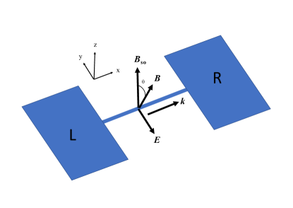
Figure 1: (color online) Sketch of the system considered. A spin-orbit active one-dimensional weak link of length $d$ is attached to two leads, $L$ and $R$. An external electric field applied in the negative $y$-direction interacts with an electron moving along the $x$-direction with momentum $k$ and generates a pseudo-magnetic field $B_{\rm so}$ in the $z$-direction. An external magnetic field B is applied in the $y-z$-plane, forming an angle $\theta$ with the $z$-direction.

Originally, the Aharonov-Casher phase AC had been predicted for a neutral particle possessing an electric moment, which moves in a magnetic field, and therefore the earlier demonstrations were accomplished on neutron and atomic interferometers (see e.g., Ref. Sangster, ). More recently this phase has been shown to induce changes in the Aharonov-Bohm oscillations observed in the magnetoconductance data taken on ring structures fabricated from HgTe/HgCdTe quantum wells, where continuously adjustable spin-orbit coupling is available Konig . However, the interpretation of such experiments relies on model calculations, and the deduction of that phase is rather indirect OEW .

In this Letter we show that the magnetoconductance anisotropy (with respect to the direction of the magnetic field) of a single weak link allows for a detailed calibration of the Aharonov-Casher phase itself. By a weak link we here mean a pseudo-one-dimensional conductor that connects two bulk conductors and dominates the electrical resistance of the system. The system we have in mind is sketched in Fig. 1. Electrons can propagate either ballistically or by tunneling through the weak link. We mainly consider the ballistic case, which is more useful in the present context, and defer a detailed discussion of the tunneling case to the supplemental material SM .

We focus specifically on weak links where the Rashba interaction Rashba is controlled by an external electric field. In the absence of a magnetic field this interaction, which preserves time-reversal symmetry, does not affect the conductance Comment . This is because the two spin projections on the direction of the pseudo magnetic field, generated by the spin-orbit interaction, are good quantum numbers and hence constants of motion of the traversing electrons. As a result, the electron transmission amplitude is diagonal in spin space and therefore the conductance does not depend on the Aharonov-Casher phase. However, by switching on an external magnetic field, which affects the dynamics of the electrons through the Zeeman interaction, time-reversal symmetry is broken and the above spin projections are no longer good quantum numbers. This makes the transmission amplitude non-diagonal and mixes the two spin projections, which correspond to different Aharonov-Casher phase factors. The ensuing interference reflects the relative orientation of the applied magnetic field ${\bf B}$ and the pseudo field ${\bf B}_{\rm so}$ generated by the SOI, giving rise to an anisotropic magnetoconductance, which depends on the product of the strength of the spin-orbit interaction and the length of the weak link, forming the Aharonov-Casher phase. Hence, measurements of the anisotropy of the magnetoconductance singles out the Aharonov-Casher phase.

Two-terminal quantum conductance of a weak link. The conductance of a conductor coupled to two terminals is given by the Landauer-Büttiker expression,

$$G=g_{0}{\rm Tr}\{{\bf t}{\bf t}^{\dagger}\}\ ,$$ (3)

$g_{0}=e^{2}/h$ being the quantum unit of conductance Meir . In general the dimension of the matrix ${\bf t}$ is twice the number of channels in the link (including the two spin projections). For a one-dimensional weak link the transmission amplitude ${\bf t}$ is a (2$\times 2$) matrix in spin space

$${\bf t}=\Gamma^{\frac{1}{2}}_{L}{\mbox{\boldmath{${\cal G}$}}}_{i}(d)\Gamma^{\frac{1}{2}}_{R}\ ,$$ (4)

where ${\mbox{\boldmath{${\cal G}$}}}_{i}(d)$ is the Green’s function (aka propagator) of the link, of length $d$, and $\Gamma_{L}$ ($\Gamma_{R}$) is the coupling to the left (right) terminal, in energy units Nikolic (these are scalars when the terminals are free electron gases).

Magnetoconductance for ballistic transport. The explicit expression for the propagator describing ballistic transport through the weak link reads Shahbazyan

$${\mbox{\boldmath{${\cal G}$}}}_{i}(d)=\frac{d}{2\pi}\int dke^{ikd}\Big{[}E_{\rm F}+i0^{+}-{\cal H}(k)\Big{]}^{-1}\ ,$$ (5)

where ${\cal H}(k)$ is the Hamiltonian of an electron moving along the weak link (assumed to lie on the $\hat{\bf x}-$ axis) with momentum ${\bf k}=k\hat{\bf x}$ (using $\hbar=1$ units)

$${\cal H}(k)=\frac{k^{2}}{2m^{\ast}}-\frac{kk_{\rm so}}{m^{\ast}}\sigma_{z}-{\bf B}\cdot{\mbox{\boldmath{$\sigma$}}}\ .$$ (6)

Here we have used that for electrons ${\mbox{\boldmath{$\mu$}}}=-\mu_{B}{\mbox{\boldmath{$\sigma$}}}$, where $\mu_{B}$ is the Bohr magneton and $\sigma$ is the vector of the Pauli matrices. The Zeeman field ${\bf B}$ (in energy units since we let $\mu_{B}=1$) lies in the $y-z$ plane, i.e., ${\bf B}=B\hat{\bf n}$ and $\hat{\bf n}=\sin(\theta)\hat{\bf y}+\cos(\theta)\hat{\bf z}$, and the pseudo magnetic field induced by the spin-orbit interaction, of strength $k_{\rm so}$ in momentum units, is along $\hat{\bf z}$. Comparing Eqs. (1) and (6) we note that $k_{\rm so}$ is proportional to the total electric field felt by the electron. It is common to extract its value from experiments, see for instance Ref. Nitta . The energy of the propagating electron is $E_{\rm F}=k^{2}_{\rm F}/(2m^{\ast})$, $m^{\ast}$ being the effective mass of the electron.

An important point of our discussion concerns the direction of the external magnetic field, ${\bf B}$. The Hamiltonian (6) shows that the effect of the spin-orbit coupling can be viewed as that of a pseudo Zeeman field which depends on the momentum and does not break time-reversal symmetry. We find below that when the external Zeeman field is parallel to this pseudo field (i.e., when $\theta=0$) the magnetoconductance of the weak link is totally devoid of the Aharonov-Casher phase. As opposed, when the Zeeman field deviates away from the $\hat{\bf z}$ direction, the magnetoconductance becomes anisotropic, with the anisotropy mainly determined by the Aharonov-Casher phase.

The integral in Eq. (5) is carried out using the Cauchy theorem SM ; Shahbazyan . It is illuminating to examine the resulting propagator for zero Zeeman field,

$${\mbox{\boldmath{${\cal G}$}}}_{i}(d,B=0)=\frac{-im^{\ast}d}{\sqrt{k^{2}_{\rm F}+k^{2}_{\rm so}}}e^{[id\sqrt{k^{2}_{\rm F}+k^{2}_{\rm so}}+ik_{\rm so}d\sigma_{z}]}\ .$$ (7)

As seen, there are two fingerprints of the spin-orbit coupling. One is of rather minor importance, the wave vector of the propagating electron is modified, $k_{\rm F}\Rightarrow\sqrt{k^{2}_{\rm F}+k^{2}_{\rm so}}$. The second is the accumulation of the Aharonov-Casher phase factor AC , $\exp(i\hat{\phi}_{\rm AC})$, where $\hat{\phi}_{\rm AC}=k_{\rm so}d\sigma_{z}$ is an operator in spin space. As explained in physical terms above, and as is obvious from Eqs. (3), (4), and (7), the phase disappears from the conductance in the absence of an external Zeeman field and one finds that

$$G(B=0)/(g_{0}\Gamma_{L}\Gamma_{R})=2(m^{\ast}d)^{2}/(k^{2}_{\rm F}+k^{2}_{\rm so})\ .$$ (8)

A Zeeman field with a component perpendicular to the pseudo field induced by the spin-orbit coupling is needed for this coupling to have any effect on the conductance.

For a magnetic field along a general direction in the $y-z$ plane, the Cauchy integration in Eq. (5) requires some care and is carried out in detail in Ref. SM . Up to second order in $B_{y}$ com1 the propagator is given by two poles at

$$k_{\pm}=\pm k_{\rm so}(1-R_{i}/2)+\widetilde{q}_{\pm}\ ,$$ (9)

where

$$\widetilde{q}^{2}_{\pm}=k_{\rm F}+k^{2}_{\rm so}\pm 2m^{\ast}B_{z}+R_{i}(k^{2}_{\rm so}\pm m^{\ast}B_{z})\ ,$$ (10)

and $R_{i}=(m^{\ast}B_{y})^{2}/[(m^{\ast}B_{z})^{2}-(k_{\rm F}k_{\rm so})^{2}]$. For zero spin-orbit coupling the propagator, and consequently the conductance, depends solely on $B=[B^{2}_{y}+B^{2}_{z}]^{1/2}$, and is isotropic with respect to the direction of the magnetic field. For $k_{\rm so}\neq 0$, it becomes anisotropic. Below, the conductance is calculated up to second order in the two magnetic field components, in particular assuming that $B_{y}\ll k_{\rm F}k_{\rm so}/m^{\ast}=v_{\rm F}k_{\rm so}=\Delta_{\rm so}/2$. The energy split caused by the spin-orbit interaction, $\Delta_{\rm so}$, is $\approx 4-5$ meV Nitta ; Heida . As the magnetic energy (with appropriate constants reinstated) is $g\mu_{B}B_{y}\sim g\,{\rm 0.06}(B_{y}/{\rm T)}\,{\rm meV}$, this inequality might be satisfied for reasonable values of the $g$-factor. (Note that the magnetic-field strength is an externally-controlled parameter.)

Following Eqs. (3) and (4), the conductance is obtained by tracing over the matrix product ${\mbox{\boldmath{${\cal G}$}}}_{i}(d){\mbox{\boldmath{${\cal G}$}}}^{\dagger}_{i}(d)$. To order $(B_{z,y}/E_{F})^{2}$ one finds that

$${\rm Tr}\{{\mbox{\boldmath{${\cal G}$}}}_{i}(d){\mbox{\boldmath{${\cal G}$}}}^{\dagger}_{i}(d)\} =\frac{2(m^{\ast}d)^{2}}{k^{2}_{\rm F}+k^{2}_{\rm so}}\Big{(}1+\Big{[}\frac{B_{z}}{E_{F}}\Big{]}^{2}\frac{k^{4}_{\rm F}}{(k^{2}_{\rm F}+k^{2}_{\rm so})^{2}}$$

$$+\Big{[}\frac{B_{y}}{E_{\rm F}}\Big{]}^{2}\frac{4k^{2}_{\rm F}+3k^{2}_{\rm so}}{4(k^{2}_{\rm F}+k^{2}_{\rm so})}-\frac{1}{2}\Big{[}\frac{B_{y}}{E_{\rm F}}\Big{]}^{2}\sin^{2}(\phi_{\rm AC})\Big{)}\ ,$$ (11)

where the Aharonov-Casher phase, equal to $\phi_{\rm AC}=k_{\rm so}d$, is the eigenvalue of $\hat{\phi}_{\rm AC}$. The normalized magnetoconductance is (assuming $k_{\rm so}\ll k_{\rm F}$)

$$\frac{G-G(B=0)}{G(B=0)}\approx\Big{[}1-\frac{2k^{2}_{\rm so}}{k^{2}_{\rm F}}\Big{]}\Big{[}\frac{B}{E_{F}}\Big{]}^{2}$$

$$+\frac{7k^{2}_{\rm so}}{4k^{2}_{\rm F}}\Big{[}\frac{B_{y}}{E_{F}}\Big{]}^{2}-\frac{1}{2}\Big{[}\frac{B_{y}}{E_{\rm F}}\Big{]}^{2}\sin^{2}(\phi_{\rm AC})\ .$$ (12)

Once the Rashba interaction is switched-on, as can be done by applying gate voltages Nitta or external electric fields Nowack , the magnetoconductance becomes anisotropic, as demonstrated by the last two terms in Eq. (12). These arise from different sources. The first one is determined by the strength of the spin-orbit coupling in the particular material forming the weak link. It is governed by the ratio $(k_{\rm so}/k_{\rm F})^{2}$, which is typically small: For the values of $k_{\rm F}=\sqrt{2\pi n_{s}}$ reported in Refs. Nitta ; Heida ($n_{s}$ is the electron density) $k_{\rm F}\approx(3-6)\times 10^{8}$ m^-1 while $k_{\rm so}$ is about two orders of magnitude smaller. Thus this material-dependent anisotropy is minute and will be neglected in what follows.

In contrast, the last term on the right hand-side of Eq. (12) provides a neat possibility to measure the Aharonov-Casher phase $\phi_{\rm AC}$ directly from the anisotropy of the magnetoconductance. To do so we normalize the measured magnetoconductance for an arbitrary angle $\theta$ between the external magnetic field [$B_{y}=B\sin(\theta)$, $B_{z}=B\cos(\theta)$] and the pseudo field induced by the spin-orbit interaction to the measured magnetoconductance for $\theta=0$. One finds that

$$\frac{G(B,\theta)-G(0,0)}{G(B,0)-G(0,0)}=1-\frac{1}{2}\sin^{2}(\theta)\,\sin^{2}(\phi_{\rm AC})\ ,$$ (13)

which is a result that only depends on the Aharonov-Casher phase $\phi_{\rm AC}$ and the angle $\theta$. This function is shown in Fig. 2.

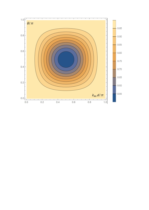
Figure 2: (color online) A contour plot of the anisotropy of the magnetoconductance for the ballistic case, as defined by Eq. (13), plotted as a function of the Aharonov-Casher phase $\phi_{\rm AC}=k_{\rm so}d$ (horizontal axis) and the angle $\theta$ between an external magnetic field and the pseudo-magnetic field generated by the spin-orbit interaction (vertical axis). The anisotropy has a maximum in the center of the contour plot, where $\phi_{\rm AC}=\theta=\pi/2$, and vanishes on the borders, where $\phi_{\rm AC}$ or $\theta$ is either 0 or $\pi$. By measuring the anisotropy at different angles $\theta$ one may determine $\phi_{\rm AC}$.

Magnetoconductance for tunneling electrons. The discussion above pertains to weak links through which electrons propagate ballistically. One may wonder what form the magnetoconductance takes for a weak link through which electron transport is by tunneling. Interestingly, the end result for the magnetoconductance anisotropy in the two cases is formally not much different. The conductances, however, are quite disparate, implying detrimental experimental consequences. Here we offer a heuristic comparison and explanations of the two scenarios.

Viewing a tunnel junction as a potential barrier whose height exceeds the energy of the impinging electrons by $E_{0}=1/(2m^{*}a_{0}^{2})$, where $a_{0}$ can be thought of as a tunneling length, the expression for the propagator is modified. We refer to Ref. SM, for a detailed derivation of the propagator ${\mbox{\boldmath{${\cal G}$}}}_{e}(d)$ and for the form of ${\rm Tr}\{{\mbox{\boldmath{${\cal G}$}}}_{e}(d){\mbox{\boldmath{${\cal G}$}}}^{\dagger}_{e}(d)\}$ for this case. To order $(B_{y,z}/E_{0})^{2}$ and for $B_{y}/E_{0}\ll k_{\rm so}a_{0}\ll 1$ one finds

$${\rm Tr}\{{\mbox{\boldmath{${\cal G}$}}}_{e}{\mbox{\boldmath{${\cal G}$}}}^{\dagger}_{e}\}=2(m^{\ast}a_{0}d)^{2}e^{-2d/a_{0}}$$

$$\times\Big{\{}1+\frac{(Bd)^{2}}{2(E_{0}a_{0})^{2}}\Big{[}1+\frac{5}{2}\frac{a_{0}}{d}+2\frac{a^{2}_{0}}{d^{2}}\Big{]}$$

$$+\frac{(B_{y}d)^{2}}{2(E_{0}a_{0})^{2}}\Big{[}\frac{a_{0}}{d}\Big{(}\frac{\sin(\phi_{\rm AC})}{\phi_{\rm AC}}-2\Big{)}+\frac{\sin^{2}(\phi_{\rm AC})}{(\phi_{\rm AC})^{2}}-1\Big{]}\Big{\}}\ .$$ (14)

The magnetoconductance is again anisotropic due to the term on the second line (which as expected vanishes if $B_{y}=0$). The magnetoconductance, normalized as in Eq. (13), becomes,

$$\frac{G(B,\theta)-G(0,0)}{G(B,0)-G(0,0)}=1-\frac{\sin^{2}(\theta)}{1+(5/2)(a_{0}/d)+2(a_{0}/d)^{2}}$$

$$\times\Big{\{}\Big{[}1-\Big{(}\frac{\sin(\phi_{\rm AC})}{\phi_{\rm AC}}\Big{)}^{2}\Big{]}+2\frac{a_{0}}{d}\Big{[}1-\frac{\sin(2\phi_{\rm AC})}{2\phi_{\rm AC}}\Big{]}\Big{\}}\ .$$ (15)

In order for the anisotropy to be determined by the single parameter $\phi_{\rm AC}=k_{\rm so}d$, the Aharonov-Casher phase, as in the ballistic case, we need $a_{0}/d\ll 1$, in which case the magnetoconductance, normalized as in Eq. (13), is

$$\frac{G(B,\theta)-G(0,0)}{G(B,0)-G(0,0)}=1-\sin^{2}(\theta)\Big{[}1-\frac{\sin^{2}(\phi_{\rm AC})}{(\phi_{\rm AC})^{2}}\Big{]}\ .$$ (16)

However, the assumption that $a_{0}/d\ll 1$ is unrealistic since that would make the conductance, which Eq. (14) shows is proportional to $\exp(-2d/a_{0})$, too small to be measured. A realistic smallest value of $\exp(-2d/a_{0})$ would be about 10^-4, corresponding to $a_{0}/d\sim 0.2$, which is a number that does not justify neglecting terms proportional to $a_{0}/d$ and $(a_{0}/d)^{2}$ in Eq. (15).

Comparing the expressions for the magnetoconductance for ballistic- and tunneling transport through a weak link, Eqs. (11) and (14), one observes that the renormalization of the electronic propagator by an external magnetic field is qualitatively different for the two transport regimes. In the ballistic transport regime the magnetic field modifies the Fermi momentum and consequently the orbital phase factors, turning $\exp[ik_{\rm F}d]$ into $\exp[ik_{\pm}d]$ [see Eqs. (7), (9), and (10)]. These orbital phase factors have no effect on the conductance. In a tunneling device, on the other hand, the magnetic field normalizes the tunneling length, introducing additional exponential dependence on the width $d$ of the tunnel junction. Such a modification affects the modulus of the propagator, and reduces further the tunneling conductance.

Discussion. We have presented an analysis of the magnetoconductance of one-dimensional weak links through which electrons propagate either ballistically (ballistic transport regime) or by tunneling (tunneling transport regime). Whether the eigenstates of the electrons in the weak link are plane waves or evanescent tunneling modes, they acquire a phase factor due to the Aharonov-Casher effect AC . The propagator matrix, written in terms of these eigenstates, is diagonal as long as the external magnetic field is parallel to the pseudo magnetic field induced by the spin-orbit coupling. In this case the conductance, given by Eqs. (3) and (4), is determined by the sum of the squared moduli of the diagonal elements of the propagator and therefore becomes independent of the Aharonov-Casher phase.

An external magnetic field that has a component perpendicular to the pseudo field, on the other hand, has the effect that spin is no longer a good quantum number, the propagator matrix becomes non-diagonal, and interference between its non-diagonal elements leads to a magnetoconductance that depends on the Aharonov-Casher phase. One can think of this as a manifestation of the Aharonov-Casher phase in the magnetoconductance due to an internal interference between spin-up and spin-down states. Our main result is Eq. (13), showing that in the ballistic transport regime this Aharonov-Casher phase can be deduced by comparing measurements of the magnetoconductance of the weak link in an external magnetic field oriented in different directions.

- (1) S. Sahoo, T. Kontos, J. Furer, C. Hoffmana, M. Gräber, A. Cottet, and C. Schönenberger, Electric field control of spin transport, Nature Phys. 1, 99 (2005).
- (2) A. Hirohata, K. Yamada, Y. Nakatani, I.-L. Prejbeanu, B. Diény, P. Pirro, and B. Hillebrands, Review on spintronics: Principles and device applications, J. Magn. Magn. Mater. 509, 166711 (2020).
- (3) J. Wunderlich, B. Kaestner, J. Sinova, and T. Jungwirth, Experimental Observation of the Spin-Hall Effect in a Two-Dimensional Spin-Orbit Coupled Semiconductor System, Phys. Rev. Lett. 94, 047204 (2005).
- (4) V. P. Amin, P. M. Haney, and M. D. Stiles, Interfacial spin-orbit torques, J. Appl. Phys. 128, 151101 (2020).
- (5) G. Bergmann, Weak anti-localizatio–An experimental proof for the destructive interference of rotated spin 1/2, Solid State Commun. 42, 815 (1982).
- (6) D. Iizasa, A. Aoki, T. Saito, J. Nitta, G. Salis, and M. Kohda, Control of spin relaxation anisotropy by spin-orbit-coupled diffusive spin motion, Phys. Rev. B 103, 024427 (2021).
- (7) Y. Aharonov and A. Casher, Topological Quantum Effects for Neutral Particles, Phys. Rev. Lett. 53, 319 (1984).
- (8) T-Z. Qian and Z-B. Su, Spin-Orbit Interaction and Aharonov-Anandan Phase in Mesoscopic Rings, Phys. Rev. Lett. 72, 2311 (1994).
- (9) J. Nitta, T. Akazaki, H. Takayanagi, and T. Enoki, Gate Control of Spin-Orbit Interaction in an Inverted In0.53Ga0.47As/In0.52Al0.48As Heterostructure, Phys. Rev. Lett. 78, 1335 (1997).
- (10) K. C. Nowack, F. H. L. Koppens, Yu. V. Nazarov, and L. M. K. Vandersypen, Coherent control of a single electron spin with electric fields , Science 318, 1430 (2007).
- (11) R. I. Shekhter, O. Entin-Wohlman, M. Jonson, and A. Aharony, Photo-spintronics of spin-orbit active electric weak links, Low Temp. Phys. 43, 910 (2017) [Fiz. Niz. Temp. 43, 1137 (2017)].
- (12) S. Varela, I. Zambrano, B. Berche, V. Mujica, and E. Medina, Spin-orbit interaction and spin selectivity for tunneling electron transfer in DNA, Phys. Rev. B 101, 241410(R) (2020).
- (13) O. Entin-Wohlman, A. Aharony, and Y. Utsumi, Comment on: ”Spin-orbit interaction and spin selectivity for tunneling electron transfer in DNA”, Phys. Rev. B 103, 077401 (2021).
- (14) Y. Utsumi, O. Entin-Wohlman, and A, Aharony, Spin selectivity through time-reversal symmetric helical junctions, Phys. Rev. B 102, 035445 (2020).
- (15) S. Takahashi and S. Maekawa, Spin current, spin accumulation and spin Hall effect, Science and Technology of Advanced Materials, 9, 014105 (2007).
- (16) A. Davidson, V. P. Amin, W. S. Aljuaid, P. M. Haney, and X. Fan, Perspectives of electrically generated spin currents in ferromagnetic materials, Phys. Letters A 384, 126228 (2020).
- (17) M. Jonson, R. I. Shekhter, O. Entin-Wohlman, A. Aharony, H. C. Park, and D. Radić, DC spin generation by junctions with AC driven spin-orbit interaction, Phys. Rev. B 100, 115406 (2019).
- (18) O. Entin-Wohlman, R. I. Shekhter, M. Jonson, and A. Aharony, Photovoltaic effect generated by spin-orbit interactions, Phys. Rev. B 101, 121303(R) (2020).
- (19) R. I. Shekhter, O. Entin-Wohlman, M. Jonson, and A. Aharony, Rashba splitting of Cooper pairs, Phys. Rev. Lett. 116, 217001 (2016); O. Entin-Wohlman, R. I. Shekhter, M. Jonson, and A. Aharony, Rashba proximity states in superconducting tunnel junctions, Low Temp. Phys. 43, 303 (2017) [Fiz. Niz. Temp. 43, 368 (2017)].
- (20) M. König, A. Tschetschetkin, E. M. Hankiewicz, J. Sinova, V. Hock, V. Daumer, M. Schäfer, C. R. Becker, H. Buhmann, and L. W. Molenkamp, Direct Observation of the Aharonov-Casher Phase, Phys. Rev. Lett. 96, 076804 (2006).
- (21) For a recent review see D. Frustaglia and J. Nitta, Geometric spin phases in Aharonov-Casher interference, Solid State Comm. 311, 113864 (2020).
- (22) E. J. Rudríguez and D. Frustaglia, Nonmonotonic quantum phase gathering in curved spintronic circuits, Phys. Rev. B 104, 195308 (2021).
- (23) A. Aharony, Y. Tokura, G. Z. Cohen, O. Entin-Wohlman, and S. Katsumoto, Filtering and analyzing mobile qubit information via Rashba-Dresselhaus-Aharonov-Bohm interferometers, Phys. Rev. B 84, 035323 (2011); S. Matityahu, A. Aharony, O. Entin-Wohlman, and C. A. Balseiro, Spin filtering in all-electrical three-terminal interferometers, Phys. Rev. B 95, 085411 (2017).
- (24) K. Sangster, E. A. Hinds, S. M. Barnett, and E. Riis, Measurement of the Aharonov-Casher phase in an atomic system, Phys. Rev. Lett. 71, 3641 (1993).
- (25) O. Entin-Wohlman and A. Aharony, DC Spin geometric phases in hopping magnetoconductance, Phys. Rev. Research 1, 033112 (2019).
- (26) See Supplemental Material at [URL will be inserted by the publisher].
- (27) E. I. Rashba, Properties of semiconductors with an extremum loop. 1. Cyclotron and combinational resonance in a magnetic field perpendicular to the plane of the loop, Fiz. Tverd. Tela (Leningrad) 2, 1224 (1960); [Sov. Phys. Solid State 2, 1109 (1960)]; Y. A. Bychkov and E. I. Rashba, Oscillatory effects and the magnetic susceptibility of carriers in inversion layers, J. Phys. C 17, 6039 (1984).
- (28) Y. Meir and N. S. Wingreen, Landauer Formula for the Current Through an Interacting Electron Region, Phys. Rev. Lett. 68, 2512 (1992).
- (29) More details of this derivation are to be found, e.g., in B. K. Nikolic, Lecture notes, Sec. 2.5.
- (30) T. V. Shahbazyan and M. E. Raikh, Low-Field Anomaly in 2D Hopping Magnetoresistance Caused by Spin-Orbit Term in the Energy Spectrum, Phys. Rev. Lett. 73, 1408 (1994).
- (31) The denominator in Eq. (5) is in general a quartic polynomial with four roots, of which two contribute to the Cauchy integration. These roots can be found analytically quite simply up to order (and to all orders in ); see Ref. SM for details.
- (32) J. P. Heida, B. J. van Wees, J. J. Kuipers, T. M. Klapwijk, and G. Borghs, Spin-orbit interaction in a two-dimensional electron gas in a InAs/AlSb quantum well with gate-controlled electron density, Phys. Rev. B 57, 11911 (1998).