Perfect Matching in Random Graphs is as Hard as Tseitin Supported by the Approximability and Proof Complexity project funded by the Knut and Alice Wallenberg Foundation.

Abstract

We study the complexity of proving that a sparse random regular graph on an odd number of vertices does not have a perfect matching, and related problems involving each vertex being matched some pre-specified number of times. We show that this requires proofs of degree $\Omega(n/\log n)$ in the Polynomial Calculus (over fields of characteristic $\neq 2$) and Sum-of-Squares proof systems, and exponential size in the bounded-depth Frege proof system. This resolves a question by Razborov asking whether the Lovász-Schrijver proof system requires $n^{\delta}$ rounds to refute these formulas for some $\delta>0$. The results are obtained by a worst-case to average-case reduction of these formulas relying on a topological embedding theorem which may be of independent interest.

1 Introduction

Proof complexity is the study of certificates of unsatisfiability, initiated by Cook and Reckhow [20] as a program to separate $\NP$ from $\coNP$. The main goal of this program is to prove size lower bounds on proofs of unsatisfiability of logical formulas. This is a daunting job – indeed we are far from proving general size lower bounds on certificates of unsatisfiability. As an intermediate step we study proof systems with restricted deductive power and prove size lower bounds for such restricted certificates of unsatisfiability. The most studied such proof system is resolution [10] which is fairly well understood by now, see e.g., the proof complexity book by Krajíček [42].

But resolution is by far not the only proof system. A closely related and quite general proof system is the bounded depth Frege proof system [20] which manipulates propositional formulas of bounded depth. While we have some results for the bounded depth Frege proof system, in this introduction we instead focus on two other systems as these were the primary motivation behind our work. These are the two proof systems Polynomial Calculus (PC) [19, 2] and Sum-of-Squares (SoS) [65, 53, 45]. These proof systems do not rely on propositional logic, like resolution or Frege, but rather on algebraic reasoning and are examples of so-called (semi-)algebraic proof systems (see e.g. [33]).

Both PC and SoS provide refutations of (satisfiability of) a set of polynomial equations $\mathcal{Q}=\{\,q_{i}(x)=0\mid i\in[m]\,\}$ over $n$ variables $x_{1},\ldots,x_{n}$. In the case of PC, these polynomials can be over any field $\mathbb{F}$ (finite or infinite), and in the case of SoS, these polynomials are over $\mathbb{R}$. A key complexity measure of a PC_F or SoS refutation of $\mathcal{Q}$ is its degree, defined as the maximum degree of any polynomial appearing in the refutation. The degree of refuting $\mathcal{Q}$ in PC_F or SoS, which we denote by $\operatorname{\sf{Deg}}(\mathcal{Q}\vdash_{\text{\tiny PC${}_{\mathbb{F}}$}}\,\perp)$ and $\operatorname{\sf{Deg}}(\mathcal{Q}\vdash_{\text{\tiny SoS}}\,\perp)$ respectively, is the minimum degree of any PC_F or SoS refutation of $\mathcal{Q}$. For Boolean systems of equations, meaning that $\mathcal{Q}$ contains the equations $x_{i}^{2}-x_{i}=0$ for all $i\in[n]$, strong enough degree lower bounds imply size lower bounds in both PC_F [19, 36] and SoS [5], where the size of a refutation is the total number of monomials appearing in it. For finite $\mathbb{F}$ the proof system PC_F is incomparable to SoS [58, 32, 33] whereas SoS can simulate PC_R by the recent result of Berkholz [9].

There is by now a large number of lower bound results for both PC [58, 36, 15, 3, 29, 50], and SoS [32, 63, 49, 6, 41, 5, 55, 1], with SoS in particular having received considerable attention in recent years due to its close connection to the Sum-of-Squares hierarchy of semidefinite programming, a powerful “meta-algorithm” for combinatorial optimization problems [7].

In this paper we study the power (or lack thereof) of these proof systems when it comes to refuting the perfect matching formula $\mathsf{PM}(G)$ defined over sparse random graphs $G=(V,E)$ on an odd number of vertices. This formula can be viewed as a system of linear equations over $\mathbb{R}$ on a set of Boolean variables: for each edge $e\in E$ there is a variable $x_{e}\in\{0,1\}$ (indicating whether the edge is used in the matching) and for each vertex $v\in V$ there is an equation $\sum_{e\ni v}x_{e}=1$. Apart from being a natural well-studied problem on its own, the perfect matching formula is interesting because of its close relation to two other widely studied families of formulas, namely the pigeonhole principle (PHP), and Tseitin formulas.

PHP asserts that $m$ pigeons cannot fit in $n<m$ holes (where each hole can fit at most one pigeon). This can be viewed as a bipartite matching problem on the complete bipartite graph with $m+n$ vertices, where each vertex on the large side (with $m$ vertices) must be matched at least once, and each vertex on the small side (with $n$ vertices) can be matched at most once. There are many variants of PHP (see e.g. the survey [59]), and the one closest to the perfect matching formula is the so-called “onto functional PHP”, in which each vertex on both sides must be matched exactly once (rather than at least/at most once). Equivalently, this formula is simply the perfect matching formula on a complete bipartite graph with $n+m$ vertices. While most variants of PHP are hard for PC [58, 50], the onto functional PHP variant is in fact easy to refute in PC over any field [60]. In SoS, all variants of PHP are easy to refute [33].

The Tseitin formula over a graph $G$ claims that there is a subgraph of $G$ such that each vertex has odd degree. As the sum of the degrees of a graph is even, this formula is not satisfiable if $G$ has an odd number of vertices. In contrast to the PHP, the Tseitin formula is (almost) always hard: for PC_F over fields $\mathbb{F}$ of characteristic distinct from 2 [15, 3] and SoS [32] these formulas require linear degree if $G$ is a good vertex expander. We cannot hope to prove degree lower bounds over fields of characteristic 2 as the constraints become linear and we can thus refute the Tseitin formula using Gaussian elimination. As the perfect matching formula $\mathsf{PM}(G)$ implies the Tseitin formula, PC over fields of characteristic $2$ can also easily refute $\mathsf{PM}(G)$ for $G$ with an odd number of vertices.

In summary, the perfect matching formula lies somewhere in between PHP and Tseitin, of which the former is easy to refute in SoS (and easy to refute in PC in the onto functional variant), and the latter is hard to refute in SoS (as well as in PC with characteristic $\neq 2$). Hence it is natural to wonder whether SoS or PC requires large degree to refute the perfect matching formula over non-bipartite graphs.

The case of perfect matching in the complete graph on an odd number of vertices (sometimes called the “MOD 2 principle”) is well-understood in both PC [15] and SoS [32, 56], requiring degree $\Omega(n)$ in both proof systems unless the underlying field of PC is of characteristic 2. For sparse graphs, less is known. Buss et al. [15] obtained worst-case lower bounds in PC showing that there exist bounded degree graphs on $n$ vertices requiring $\Omega(n)$ degree refutations. This is obtained by a reduction from Tseitin formulas and while the work of Buss et al. predates the current interest in the SoS system, it is not hard to see that the same reduction yields a similar $\Omega(n)$ degree lower bound for SoS (details provided in Appendix A).

However, for random graphs $G$ little is known about the hardness of the perfect matching formula and, e.g., Razborov [57] asked whether it is true that the Lovász-Schrijver hierarchy [47] (which is weaker than SoS) requires $n^{\varepsilon}$ rounds to refute the perfect matching principle on a random sparse regular graph with high probability.

1.1 Our results

We show that indeed the perfect matching principle requires large size on random $d$-regular graphs (for some constant $d$) in the Sum-of-Squares, Polynomial Calculus, and bounded-depth Frege proof systems. Our results apply more generally to Tseitin-like formulas defined by linear equations over the reals induced by some graph, so let us now define these.

For a graph $G=(V,E)$ and integer vector $b\in\mathbb{Z}^{V}$, consider the system of linear equations over the reals having a variable $x_{e}$ for each $e\in E$, and the equation $\sum_{e\ni v}x_{e}=b_{v}$ for each $v\in V$. Let $\operatorname{Card}(G,b)$ denote this system of linear equations along with the Boolean constraints $x_{e}\in\{0,1\}$ (viewed as a quadratic equation $x_{e}^{2}-x_{e}=0$) for each edge – in Section 2.2 the encoding is discussed in more detail. Note that $\operatorname{Card}(G,\vec{1})$ corresponds to the perfect matching problem in $G$ and in general $\operatorname{Card}(G,b)$ can be viewed as asserting that $G$ has a “matching” where each vertex is matched exactly $b_{v}$ times. Note that whenever $\sum_{v\in V}b_{v}$ is odd, $\operatorname{Card}(G,b)$ is unsatisfiable (since the equations imply $\sum_{v}b_{v}=2\sum_{e}x_{e}$ which is even).

We focus on the special case of $\operatorname{Card}(G,b)$ where $G$ is $d$-regular and $b=\vec{t}=(t,t,\ldots,t)$ is the all-$t$ vector for some $t\in[d]$. If in this scenario both $n$ and $t$ are odd (implying $d$ is even) then as observed above $\operatorname{Card}(G,\vec{t})$ is unsatisfiable. On the other hand if $n$ is odd and $t$ is even then $\operatorname{Card}(G,\vec{t})$ is always satisfiable (because such $G$ admits a $2$-factorization). The remaining case when $n$ is even may be either satisfiable or unsatisfiable, but for a random $d$-regular $G$ with $d\geq 3$, $\operatorname{Card}(G,t)$ will be satisfiable with high probability (because such $G$ can be partitioned into perfect matchings with high probability).

If we let $\mathscr{F}_{{D}}$ denote a Frege system restricted to depth-$D$ formulas (see Section 2.1), then our main theorem is as follows.

Theorem 1.1.

There is a constant $d_{0}$ such that for all constants $d\geq d_{0}$ and $t\in[d]$, the following holds asymptotically almost surely over a random $d$-regular graph $G$ on $n$ vertices.

1. $\operatorname{\sf{Deg}}(\operatorname{Card}(G,\vec{t})\vdash_{\text{\tiny PC${}_{\mathbb{F}}$}}\,\perp)=\Omega(n/\log n)$ for any fixed field $\mathbb{F}$ with $\operatorname{char}(\mathbb{F})\neq 2$.

2. $\operatorname{\sf{Deg}}(\operatorname{Card}(G,\vec{t})\vdash_{\text{\tiny SoS}}\,\perp)=\Omega(n/\log n)$.

3. There is a $\delta>0$ such that $\operatorname{\sf{Size}}(\operatorname{Card}(G,\vec{t})\vdash_{\text{\tiny$\mathscr{F}_{{D}}$}}\,\perp)=\exp\big{(}\Omega(n^{\delta/D})\big{)}$, for all $D\leq\frac{\delta\log n}{\log\log n}$.

The interesting case of the above theorem is when both $n$ and $t$ are odd so that $\operatorname{Card}(G,t)$ is unsatisfiable; in the other cases $\operatorname{Card}(G,\vec{t})$ is satisfiable with high probability and the lower bounds are vacuous.

By known size-degree tradeoffs for Polynomial Calculus [36, 19] and Sum-of-Squares [5] the degree lower bounds in Theorem 1.1 imply near-optimal size lower bounds of $\exp\big{(}\Omega(n/\log^{2}n)\big{)}$.

Apart from the perfect matching formula, another special case of $\operatorname{Card}(G,\vec{t})$ is the so-called even coloring formula, introduced by Markström [48], which is the case when $t=\deg(v)/2$. An open problem of Buss and Nordström [16, Open Problem 7.7] asks whether these formulas are hard on spectral expanders for Polynomial Calculus over fields of characteristic $\neq 2$. Theorem 1.1 partially resolves this open problem, establishing that it is hard on random graphs (rather than on all spectral expanders). See Section 6 for some further remarks on what parts of our proof use the randomness assumption.

We will give a more detailed overview of how the results are obtained in Section 1.3 below, but for now let us mention that we obtain them using embedding techniques, as introduced to proof complexity by Pitassi et al. [54] (see discussion of related work in Section 1.2). In particular for, say, the SoS lower bound, our starting point is the $\Omega(n)$ worst-case degree lower bound in sparse graphs, and we then prove that these hard instances can be embedded in a random $d$-regular graph in such a way that the hardness of refuting the formula is preserved.

To achieve this, one of the components we need is a new graph embedding theorem which may be of independent interest. Very loosely speaking, we show that any bounded-degree graph with $O(n/\log n)$ edges can be embedded as a topological minor in any bounded-degree $\alpha$-expander on $n$ vertices and sufficiently many edges. In addition, for our application to perfect matching (and more generally the $\operatorname{Card}(G,\vec{t})$ formulas), we need to be able to control the parities of the path lengths used in the topological embedding, and we show that as long as every large linear-sized subgraph contains an odd cycle of length $\Omega(1/\alpha)$, this is indeed possible.

Somewhat informally, we prove the following.

Theorem 1.2 (Informal statement of Theorem 3.3).

Let $G$ be a constant degree $\alpha$-expander on $n$ vertices. If $H$ is a graph with at most $\frac{\varepsilon n}{\log n}$ edges and $\Delta(H)\ll\alpha^{2}\cdot d(G)$, then $G$ contains $H$ as a topological minor. Furthermore, if all large vertex induced subgraphs of $G$ contain an odd cycle of length $\Omega(1/\alpha)$, then one can choose the parities of the length of all the edge embeddings in the minor.

This generalizes various classical results of a similar flavor (e.g. [39, 44, 18, 43]). See the next subsection for a discussion comparing these (and other) existing embedding results to ours.

As a further illustration of the applicability of this theorem we partially resolve a question of Filmus et al. [24]. They prove that with high probability for random $d$-regular graphs $G$, where $d\geq 4$, PC requires space $\Omega(\sqrt{n})$ to refute the Tseitin formula, and conjecture that PC in fact requires space $\Omega(n)$. On the other hand, Galesi et al. [28] considered it plausible that the $\Omega(\sqrt{n})$ bound is optimal. We (almost) resolve this question by proving $\Omega(n/\log n)$ space lower bounds for the Tseitin formula defined on vertex expanders, but only of large enough (constant) average degree.

Theorem 1.3.

For all $\alpha>0$ there is a $d_{0}$ such that the following holds. Let $G$ be a bounded degree $\alpha$-expander on $n$ vertices of average degree at least $d_{0}$. Then over any field $\mathbb{F}$ it holds that PC_F requires space $\Omega(n/\log n)$ to refute the Tseitin formula defined on $G$.

Let us mention that the constant hidden in the lower bound $\Omega(n/\log n)$ depends on the maximum degree of $G$. Unlike Theorem 1.1, vertex expansion is sufficient and we require no randomness. This lower bound is obtained by embedding a worst-case instance, due to Filmus et al., into a vertex expander. We provide more details in Section 6.1.

1.2 Related work

Proof Complexity Lower Bounds Using Embedding Techniques

There are a few other papers that employ embedding techniques in proof complexity [54, 31, 27, 37], though none of these use the embedding techniques in connection with algebraic systems like PC or SoS. As far as we are aware the first such work is that of Pitassi et al. [54], who apply embedding techniques to obtain Tseitin lower bounds for Frege Systems, and their use is most similar to ours. They rely on a result of Kleinberg and Rubinfeld [39] that guarantees that any small enough graph is a minor of an expander (note that we require topological minors). This is in contrast to the other results that rely on the fundamental result that a graph of large enough treewidth contains the grid graph as a minor [61].

Connection to Constraint Satisfaction Problems

For a $k$-ary predicate $P:\{0,1\}^{k}\rightarrow\{0,1\}$, an instance of the $\operatorname{CSP}(P)$ problem consists of a set of constraints over $n$ Boolean variables $x_{1},\ldots,x_{n}$, each constraint being an application of $P$ on a list of $k$ variables. The $\operatorname{Card}(G,\vec{t})$ formulas we study can be viewed as instances of $\operatorname{CSP}(P)$ where each variable appears in exactly two constraints and $P:\{0,1\}^{d}\rightarrow\{0,1\}$ is the constraint that exactly $t$ of the $d$ inputs are $1$.

CSP problems have been extensively studied throughout the years, and fairly general conditions under which $\operatorname{CSP}(P)$ is hard for PC and SoS are known [3, 41]. To be more accurate, these results are for the more general $\operatorname{CSP}(P^{\pm})$ problem in which each constraint is an application of $P$ on $k$ literals rather than variables. In particular, Alekhnovich and Razborov [3] showed that if $P$ is, say, $8$-immune over the underlying field $\mathbb{F}$, then any PC_F refutation of a random $\operatorname{CSP}(P^{\pm})$ instance with a linear number of constraints requires degree $\tilde{\Omega}(n)$. For SoS, Kothari et al. [41] showed that, if there exists a pairwise uniform distribution $\mu$ over $\{0,1\}^{k}$ supported on satisfying assignments of $P$, then with high probability a random $\operatorname{CSP}(P^{\pm})$ instance on $m=\Delta n$ constraints needs degree $\tilde{\Omega}(n/\Delta^{2})$ to be refuted by the SoS proof system.

The predicates we study are linear equations over $\mathbb{R}$ and are neither immune nor do they support a pairwise uniform distribution. As such, our results provide CSP lower bounds that fall outside the immunity and pairwise independence frameworks, which are the source of a majority of existing CSP lower bounds in PC and SoS. To the authors’ best knowledge the only other attempt to overcome this framework in the average-case setting is the paper by Deshpande et al. [21], showing lower bounds for the basic SDP of random regular instances of $\operatorname{CSP}(\operatorname{NAE}_{3}^{\pm})$, where $\operatorname{NAE}_{3}$ is the not-all-equal predicate on three bits. In contrast to their work we show (almost) linear degree lower bounds for the stronger Sum-of-Squares hierarchy, but only for a very wide predicate of some large (but constant) arity.

Embedding Theorems

There is a rich literature on embeddings of graphs as minors or topological minors into expander graphs. We focus here on the ones most closely related to Theorem 1.2.

The classical result of Kleinberg and Rubinfeld [39] shows that a regular expander $G$ on $n$ vertices contains every graph $H$ with $O(n/\polylog(n))$ vertices and edges as a minor. Krivelevich and Nenadov [44] simplified and strengthened this by improving the bound on the size of $H$ to $O(n/\log n)$. These results differ from ours in two key ways: (i) we want topological minors, and (ii) we want to be able to control the parities of the path lengths in the embedding. We now discuss these two aspects separately.

Results on topological minors, while somewhat less common, also exist. A result similar to ours is the result of Broder et al. [13] that with high probability the random graph $\mathcal{G}(n,m)$ on $n$ vertices and $m=\Omega(n\log n)$ edges contains any graph $H$ with $\Delta(H)=O(m/n)$ and at most $O(n/\log n)$ edges (and at most $n/2$ vertices) as a topological minor.

For our second property, the possibility to choose the parities of the paths used in the topological embedding, we are not aware of any previous work studying this question. A related notion are so called odd minors which are more general than topological minors with odd length paths. This notion has been considered in connection with a strengthening of Hadwiger’s Conjecture, see e.g., the survey by Seymour [64]. This line of research mostly considers complete odd minors, e.g., [30], and thus is not directly applicable to our situation.

Recently Draganić et al. [22] independently obtained a new embedding theorem similar to ours. They assume the somewhat stronger property that the host graph $G$ is a spectral expander but also obtain a stronger conclusion: each path of the topological embedding is of equal (odd) length and the embedding even works in an adversarial setting. Namely, the adversary is allowed to fix the embedding of the vertices, as long as no neighborhood in $G$ contains too many vertex embeddings.

The embedding theorem of Draganić et al. can be used to implement our proof strategy. The results are unaffected by this change except in the setting of Theorem 1.3. There, instead of considering vertex expanders, we need to consider regular spectral expanders with the benefit that the required average degree $d_{0}$ is considerably decreased.

Extended Formulations

There has been a fair amount of work studying the extension complexity of the perfect matching polytope [67, 62], but these lower bounds do not have any direct implications for the PC and SoS degree of the perfect matching formula. Let us elaborate.

Suppose we have a convex polytope $\mathcal{P}$ consisting of many facets. A natural question is whether there is simpler polytope $\mathcal{Q}$ in a higher dimensional space so that $\mathcal{P}$ is the “shadow” of $\mathcal{Q}$, or a bit more formally that there is a linear projection $\pi$ such that $\pi(\mathcal{Q})=\mathcal{P}$. Such a $\mathcal{Q}$ is then called a linear extension of $\mathcal{P}$ and the extension complexity of a polytope $\mathcal{P}$ is the minimum number of facets of any linear extension of $\mathcal{P}$.

Rothvoss [62] proved that the perfect matching polytope of a complete $n$-node graph has extension compexity $\exp(\Omega(n))$ for $n$ even. This result is incomparable to our lower bounds: as the graphs we consider do not contain a perfect matching, their perfect matching polytope is empty and thus has extension complexity 0. Rather than linear programs, i.e., polytopes, we consider semidefinite programs which are more expressive. The extension complexity in the semidefinite setting has also been studied before [46, 12] but these results are incomparable for the same reason just mentioned. While these results are incomparable, it is worth mentioning that there is a connection between Sherali-Adams (a proof system weaker than SoS) and extended formulations [17, 40].

1.3 Overview of Proof Techniques

As previously mentioned, our high level approach is to first obtain worst-case perfect matching lower bounds and to then embed these into the $\operatorname{Card}(G,\vec{t})$ formula for $G$ a random regular graph. The worst-case lower bounds are obtained by a gadget reduction from Tseitin to perfect matching, due to Buss et al. [15]. Using known lower bounds for the Tseitin formula in the corresponding proof systems [15, 32, 34] we then obtain the desired worst-case lower bounds for the perfect matching formula.

A naïve attempt to obtain average-case lower bounds from a sparse worst-case instance $H$ on $n$ vertices is to topologically embed the worst-case instance into a random regular graph $G$ on $O(n\log n)$ vertices using Theorem 1.2. One would then like to argue that $\mathsf{PM}(G)$ is hard.

Suppose each path $p_{uv}$ in the embedding of $H$ in $G$ corresponding to some edge $\{u,v\}\in E(H)$ is of odd length. Then it is straightforward to verify that the perfect matching formula defined over the embedding is at least as hard to refute as the worst-case instance $\mathsf{PM}(H)$: map each variable $y_{e}$, for $e\in p_{uv}$, alternatingly to $x_{uv}$ or $\bar{x}_{uv}$ such that the first and last edges of $p_{uv}$ are mapped to $x_{uv}$ (using that $p_{uv}$ is of odd length). This simple projection maps the perfect matching formula defined over the embedding of $H$ to $\mathsf{PM}(H)$ and thus shows that the hardness of $\mathsf{PM}(H)$ should be inherited.

But having such a worst-case instance as a topological minor is not sufficient to conclude that $\mathsf{PM}(G)$ is hard. For instance $G$ may contain an isolated vertex and it is then trivial to refute $\mathsf{PM}(G)$. On the other hand if we could guarantee that there is a perfect matching $m$ in the subgraph of $G$ induced by the vertices not used in the embedding of $H$, we can conclude that $\mathsf{PM}(G)$ is hard: hit the formula with the restriction corresponding to the matching $m$ and by the argument from the previous paragraph we are basically left with the worst-case formula.

Thus if we can ensure that $H$ is a topological minor of $G$ with the two additional properties that (i) every path used in the embedding of $H$ has odd length, and (ii) there exists a perfect matching in the subgraph of $G$ induced by the vertices not used in the embedding of $H$, then we obtain average-case lower bounds for the perfect matching formula $\mathsf{PM}(G)\equiv\operatorname{Card}(G,\vec{1})$. The lower bounds for $\operatorname{Card}(G,\vec{t})$ for $t>1$ can then be obtained by a reduction to the $t=1$ case: after fixing the value of the edges in $\lfloor t/2\rfloor$ cycle covers of $G$ to $1$, a restriction of $\operatorname{Card}(G,\vec{t})$ is obtained which behaves like $\operatorname{Card}(G^{\prime},\vec{1})$ for a somewhat sparser random regular graph $G^{\prime}$.

Let us elaborate a bit further on the properties required from the topological minor of $H$ in $G$. As mentioned previously, our embedding theorem can ensure that all paths are of odd length. To ensure the second property, we in fact do not embed $H$ directly into $G$ but rather into a suitably chosen vertex induced subgraph $G[T]$ with the crucial property that for any set of vertices $U\subseteq T$ of odd cardinality the induced subgraph $G[V\setminus U]$ has a perfect matching. As the embedding of $H$ will consist of an odd number of vertices we then obtain property (ii) above. Since we now want to apply Theorem 1.2 not to $G$ but to $G[T]$, we have to ensure that $G[T]$ satisfies all the conditions of that theorem. We prove what we refer to as the Partition Lemma, which asserts that an induced subgraph $G[T]$ exists that satisfies both the perfect matching property described above, as well as all conditions of Theorem 1.2. The proof of the Partition Lemma relies primarily on the Lovász Local Lemma and spectral bounds to obtain the desired properties.

For the proof of our embedding theorem (Theorem 1.2), we extend an argument due to Krivelevich and Nenadov [44] (see also [43]) for ordinary minors (rather than topological minors). In order to obtain a minor embedding of $H$ in $G$, the idea there is to embed the vertices one by one from $H$ in $G$ while maintaining an “unused” subgraph $G^{\prime}$ of $G$ which is a slightly worse expander than $G$ is. During this process it may happen that some vertex embedding cannot be connected to a neighbor. If this happens, the embedding of that vertex is removed and it needs to be embedded again.

In order to obtain topological embeddings, we need to adapt this procedure. Since we now want vertex-disjoint paths connecting the embedded vertices, we would ideally like to embed each vertex of $H$ as a large star, and then embed the edges of $H$ as paths connecting different leaves of these stars. In order to make this work out, rather than embedding the vertices as actual stars, we embed them as “star-like” subgraphs of $G$ (more precisely defined in Definition 5.4) that consist of a central vertex connected to many large vertex-disjoint connected subgraphs of $G$ and show (Lemma 5.5) that we can always embed the vertices of $H$ as such “star-like” subraphs of $G$.

With this in place, obtaining control of the parities of the path lengths used in the embedding (under the assumption on odd cycles in Theorem 1.2) is relatively straightforward: almost by definition, when embedding an edge of $H$ into a path of $G$, we can route it via an odd cycle and can then choose which of the two halves of the odd cycles to use, obtaining two possible embeddings with different path length parity, and can choose the one with the appropriate parity.

1.4 Organization

We give some preliminaries in Section 2, formally defining the used proof systems and encodings used, and recalling some general background results. In Section 3 we provide most of the proof of Theorem 1.1 while deferring the proofs of two key results, the aforementioned Partition Lemma and our embedding theorem. The proof of the Partition Lemma is given in Section 4, and the proof of the embedding theorem can be found in Section 5.

In Appendix A we recall the reduction of Buss et al. [15] from Tseitin to perfect matching and show that it yields lower bounds not only for Polynomial Calculus but also for Sum-of-Squares and bounded depth Frege.

2 Preliminaries

Natural logarithms (base $\mathrm{e}$) are denoted by $\ln$, whereas base $2$ logarithms are denoted by $\log$. For integers $n\geq 1$ we introduce the shorthand $[n]=\{1,2,\ldots,n\}$ and sometimes identify singletons $\{u\}$ with the element $u$. For a set $U$ we denote the power set of $U$ by $2^{U}$ and a transversal $A$ of a family of sets $\mathcal{B}=\{B_{1},B_{2},\ldots B_{n}\}$ is a set such that there is a bijective function $f:A\to\mathcal{B}$ satisfying that $a\in f(a)$ for all elements $a\in A$.

2.1 Proof Systems

Let $\mathcal{P}=\{p_{1}=0,\ldots,p_{m}=0\}$ be a system of polynomial equations over the set of variables $X=\{x_{1},\ldots,x_{n},\bar{x}_{1},\ldots,\bar{x}_{n}\}$. Each $p_{i}$ is called an axiom, and throughout the paper we always assume $\mathcal{P}$ includes all axioms $x_{i}^{2}-x_{i}$ and $\bar{x}_{i}^{2}-\bar{x}_{i}$, ensuring that the variables are boolean, as well as the axioms $1-x_{i}-\bar{x}_{i}$, making sure that the “bar” variables are in fact the negation of the “non-bar” variables.

Sum-of-Squares (SoS)

is a static semi-algebraic proof system. An SoS proof of $f\geq 0$ from $\mathcal{P}$ is a sequence of polynomials $\pi=(t_{1},\ldots,t_{m};s_{1},\ldots,s_{a})$ such that

$$\sum_{i\in[m]}t_{i}p_{i}+\sum_{i\in[a]}s^{2}_{i}=f\enspace.$$ (1)

The degree of a proof $\pi$ is

$$\operatorname{\sf{Deg}}(\pi)=\max\{\max_{i\in[m]}\deg(t_{i})+\deg(p_{i}),\max_{i\in[a]}2\deg(s_{i})\}\enspace.$$ (2)

An SoS refutation of $\mathcal{P}$ is an SoS proof of $-1\geq 0$ from $\mathcal{P}$, and the SoS degree to refute $\mathcal{P}$ is the minimum degree of any SoS refutation of $\mathcal{P}$: if we let $\pi$ range over all SoS refutations of $\mathcal{P}$, we can write $\operatorname{\sf{Deg}}(\mathcal{P}\vdash_{\text{\tiny SoS}}\,\perp)=\min_{\pi}\operatorname{\sf{Deg}}(\pi)$.

Definition 2.1 (Pseudoexpectation).

A degree $d$ pseudo-expectation for $\mathcal{P}$ is a linear operator $\tilde{\mathbb{E}}$ on the space of real polynomials of degree at most $d$, such that

1. $\tilde{\mathbb{E}}[1]=1$,

2. $\tilde{\mathbb{E}}[tp]=0$ for all polynomials $t$ and $p\in\mathcal{P}$ with $\deg(t)+\deg(p)\leq d$, and

3. $\tilde{\mathbb{E}}[s^{2}]\geq 0$ for all polynomials $s$ of degree $\deg(s)\leq d/2$.

It is easy to check that if there is a degree $d$ pseudo-expectation for $\mathcal{P}$, then there is no SoS refutation of $\mathcal{P}$ of degree at most $d$: if $\tilde{\mathbb{E}}$ is applied to both sides of (1), where $f=-1$, then the right side is equal to $-1$ while the left is greater than or equal to $0$.

The size of an SoS refutation $\pi$, $\operatorname{\sf{Size}}(\pi)$, is the sum of the number of monomials in each polynomial in $\pi$ and the size of refuting $\mathcal{P}$ is the minimum size over all refutations $\operatorname{\sf{Size}}(\mathcal{P}\vdash_{\text{\tiny SoS}}\,\perp)=\min_{\pi}\operatorname{\sf{Size}}(\pi)$.

Polynomial Calculus

is a dynamic proof system operating on polynomial equations over a field $\mathbb{F}$. Let $\mathcal{P}$ be over $\mathbb{F}$. Polynomial Calculus over $\mathbb{F}$ (PC_F) consists of the derivation rules

• linear combination   $p=0$         $q=0$        $\alpha p+\beta q=0$ , where $p,q\in\mathbb{F}[X]$ and $\alpha,\beta\in\mathbb{F}$, and

• multiplication    $p=0$     $xp=0$ , where $p\in\mathbb{F}[X]$ and $x\in X$.

A PC refutation of $\mathcal{P}$ is a sequence of polynomials $\pi=t_{1},\ldots,t_{\ell}$ such that $t_{\ell}=1$ and each polynomial $t_{i}$ is either in $\mathcal{P}$ or can be derived by one of the derivation rules from earlier polynomials. The degree of a refutation is the maximum degree appearing in the sequence $\operatorname{\sf{Deg}}(\pi)=\max_{i\in[\ell]}\operatorname{\sf{Deg}}(t_{i})$ and the PC_F degree of refuting $\mathcal{P}$ is the minimum degree required of any refutation $\operatorname{\sf{Deg}}(\mathcal{P}\vdash_{\text{\tiny PC${}_{\mathbb{F}}$}}\,\perp)=\min_{\pi}\operatorname{\sf{Deg}}(\pi)$. Similarly, the size of a refutation $\pi$ is the sum of the number of monomials in each line of $\pi$ and the PC_F size of refuting $\mathcal{P}$ is the minimum size required of any refutation $\operatorname{\sf{Size}}(\mathcal{P}\vdash_{\text{\tiny PC${}_{\mathbb{F}}$}}\,\perp)=\min_{\pi}\operatorname{\sf{Size}}(\pi)$.

Frege System

Let us describe a Frege system due to Shoenfield, as presented in [66]. As Frege systems over the basis $\lor$, $\land$ and $\lnot$ can polynomially simulate each other [20], the details of the system are not essential and hold for any Frege system over the mentioned basis.

Schoenfield’s Frege system works over the basis $\lor$ and $\lnot$. We treat the conjunction $A\land B$ as an abbreviation for the formula $\lnot(\lnot A\lor\lnot B)$ and let 0, 1 denote “false” and “true” respectively. If $A$ is a formula over variables $p_{1},\ldots,p_{m}$, and $\sigma$ maps the variables $p_{1},\ldots,p_{m}$ to formulas $B_{1},\ldots,B_{m}$, then $\sigma(A)$ is the formula obtained from $A$ by replacing the variable $p_{i}$ with $B_{i}=\sigma(p_{i})$ for all $i\in[m]$.

A rule is a sequence of formulas written as $A_{1},\ldots,A_{k}\vdash A_{0}$. If every truth assignment satisfying all of $A_{1},\ldots,A_{k}$ also satisfies $A_{0}$, then the rule is sound. A formula $C_{0}$ is inferred from $C_{1},\ldots,C_{k}$ by the rule $A_{1},\ldots,A_{k}\vdash A_{0}$ if there is a function $\sigma$ mapping the variables $p_{1},\ldots,p_{m}$, over which $A_{0},\ldots,A_{k}$ are defined, to formulas $B_{1},\ldots,B_{m}$ such that for all $i\in\{0,\ldots,k\}$ it holds that $C_{i}=f(A_{i})$.

The Frege system $\mathscr{F}$ that we consider consists of the following rules:

$$\vdash p\lor\lnot p$$ Excluded Middle,

$$p \vdash q\lor p$$ Expansion rule,

$$p\lor p \vdash p$$ Contraction rule,

$$p\lor(q\lor r) \vdash(p\lor q)\lor r$$ Associative rule,

$$p\lor q,\lnot p\lor r \vdash q\lor r$$ Cut rule.

An $\mathscr{F}$-refutation of an unsatisfiable formula $A=C_{1}\land\ldots\land C_{m}$ is a sequence of formulas $F_{1},F_{2},\ldots,F_{\ell}$ such that $F_{\ell}=0$ and every formula $F_{i}$ is either one of $C_{1},\ldots,C_{m}$ or inferred from formulas $F_{j_{1}},\ldots,F_{j_{k}}$ earlier in the sequence by a rule in $\mathscr{F}$. As $\mathscr{F}$ is sound and complete a formula $A$ has a refutation if and only if it is unsatisfiable.

The size of a formula is the number of connectives in the formula and the size of a refutation $\pi$, denoted by $\operatorname{\sf{Size}}(\pi)$, is the sum of the sizes of all formulas in the refutation. The depth of $\pi$ is the maximum depth of any formula $F\in\pi$. We denote by $\mathscr{F}_{{d}}$ the proof system $\mathscr{F}$ restricted to formulas of depth at most $d$.

2.2 Propositional Formulas

As we are only interested in constant degree graphs all our axioms are of constant size. Hence the precise encoding of the axioms is not significant as we can change the encoding in constant size/degree.

As the encoding is not essential, we view a propositional formula $\mathcal{F}$ over the Boolean variables $x_{1},\ldots,x_{n}$ as a family of functions $\mathcal{F}=\{f_{1},\ldots,f_{m}\}$ where each $f_{i}:\{0,1\}^{n}\to\{\text{True},\text{False}\}$ is a function that depends on a constant number of variables. The formula $\mathcal{F}$ is satisfied by an assignment $\alpha\in\{0,1\}^{n}$ if under $\alpha$ all functions evaluate to True: $f_{i}(\alpha)=\text{True}$ for all $i\in[m]$.

For a map $\rho:\{x_{1},\ldots,x_{n}\}\to\{0,1,x_{1},\ldots,x_{n},\bar{x}_{1},\ldots,\bar{x}_{n}\}$ and a function $f:\{0,1\}^{n}\to\{\text{True},\text{False}\}$, denote by ${\left.\kern-1.2ptf\vphantom{\big{|}}\right|_{\rho}}$ the function defined by ${\left.\kern-1.2ptf\vphantom{\big{|}}\right|_{\rho}}(x_{1},\ldots,x_{n})=f(\rho(x_{1}),\ldots,\rho(x_{n}))$. We extend this notation to formulas in the obvious way, i.e., ${\left.\kern-1.2pt\mathcal{F}\vphantom{\big{|}}\right|_{\rho}}=\{{\left.\kern-1.2ptf_{1}\vphantom{\big{|}}\right|_{\rho}},{\left.\kern-1.2ptf_{2}\vphantom{\big{|}}\right|_{\rho}},\ldots,{\left.\kern-1.2ptf_{m}\vphantom{\big{|}}\right|_{\rho}}\}$.

Two formulas $\mathcal{F}$ and $\mathcal{F}^{\prime}$ are equivalent, denoted by $\mathcal{F}\equiv\mathcal{F}^{\prime}$ if the formulas are element-wise equivalent, disregarding functions that are constant True. We say that a formula $\mathcal{F}^{\prime}$ is an affine restriction of $\mathcal{F}$ if there is a map $\rho:\{x_{1},\ldots,x_{n}\}\to\{0,1,x_{1},\ldots,x_{n},\bar{x}_{1},\ldots,\bar{x}_{n}\}$ such that $\mathcal{F}^{\prime}\equiv{\left.\kern-1.2pt\mathcal{F}\vphantom{\big{|}}\right|_{\rho}}$. The following lemma states that a formula $\mathcal{F}$ is at least as hard as any of its affine restrictions.

Lemma 2.2.

Let $\mathcal{F},\mathcal{F}^{\prime}$ be formulas such that $\mathcal{F}^{\prime}$ is an affine restriction of $\mathcal{F}$ and each axiom of $\mathcal{F}$ depends on a constant number of variables. Then,

1. for any field $\mathbb{F}$ it holds that $\operatorname{\sf{Deg}}(\mathcal{F}\vdash_{\text{\tiny PC${}_{\mathbb{F}}$}}\,\perp)\in\Omega\big{(}\operatorname{\sf{Deg}}(\mathcal{F}^{\prime}\vdash_{\text{\tiny PC${}_{\mathbb{F}}$}}\,\perp)\big{)}$,

2. $\operatorname{\sf{Deg}}(\mathcal{F}\vdash_{\text{\tiny SoS}}\,\perp)\in\Omega\big{(}\operatorname{\sf{Deg}}(\mathcal{F}^{\prime}\vdash_{\text{\tiny SoS}}\,\perp)\big{)}$, and

3. for all $d\geq 2$ it holds that $\operatorname{\sf{Size}}(\mathcal{F}\vdash_{\text{\tiny$\mathscr{F}_{{d}}$}}\,\perp)\in\Omega\big{(}\operatorname{\sf{Size}}(\mathcal{F}^{\prime}\vdash_{\text{\tiny$\mathscr{F}_{{d+1}}$}}\,\perp)\big{)}$.

Proof 2.3.

Suppose we have a refutation $\pi$ of $\mathcal{F}$ in one of the mentioned proof systems. We want to show that if we hit the proof with the restriction $\rho$ such that ${\left.\kern-1.2pt\mathcal{F}\vphantom{\big{|}}\right|_{\rho}}\equiv\mathcal{F}^{\prime}$ then we obtain a proof $\pi^{\prime}={\left.\kern-1.2pt\pi\vphantom{\big{|}}\right|_{\rho}}$ of $\mathcal{F}^{\prime}$.

First we need to ensure that we can derive all the axioms of $\mathcal{F}^{\prime}$. These may be encoded in a different manner, but as these proof systems are implicationally complete, and each axiom only depends on a constant number of variables, this can be done in constant degree (constant size).

This shows that the SoS degree of the resulting refutation is at most a constant factor larger. For Polynomial Calculus and Frege the statement is readily verified by an inductive argument over the proof.

For concreteness let us also define the encoding of the formulas that we are interested in.

Perfect Matching and $\operatorname{Card}(G,\vec{b})$

The Perfect Matching formula $\mathsf{PM}(G)$ encodes the claim that the graph $G$ contains a perfect matching. For every edge $e\in E(G)$ introduce a boolean variable $x_{e}\in\{0,1\}$ and add for every vertex $v\in V(G)$ an axiom claiming that precisely one incident edge is set to true. As a polynomial over $\mathbb{R}$, we encode this claim as

$$q^{\mathsf{PM}}_{v}=\sum_{e\ni v}x_{e}-1\enspace,$$ (3)

which is satisfied under an assignment $\alpha$ if $q^{\mathsf{PM}}_{v}(\alpha)=0$. Over other fields we encode this as a sum over indicator polynomials (see example for Tseitin below). For the Frege proof system we encode the vertex axiom as the propositional formula

$$q^{\mathsf{PM}}_{v}=\bigvee_{e\ni v}x_{e}\wedge\bigwedge_{\begin{subarray}{c}e,e^{\prime}\ni v\\ e\neq e^{\prime}\end{subarray}}\bar{x}_{e}\vee\bar{x}_{e^{\prime}}\enspace.$$ (4)

The formula $\operatorname{Card}(G,\vec{b})$ is encoded in a similar fashion: in the polynomial encoding replace the 1 with $b_{v}$, whereas in the propositional encoding we let the latter $\wedge$ range over edge-tuples of size $b_{v}+1$.

Tseitin Formula

The Tseitin formula $\tau(G)$ claims that the edges of the graph $G$ can be labeled by $0,1$ such that the number of 1-labeled edges incident to any vertex is odd. For every edge $e\in E(G)$ introduce a boolean variable $y_{e}\in\{0,1\}$, denote the set of variables corresponding to edges incident to $v$ by $Y_{v}=\{y_{e}\mid v\in e\}$ and let $A_{v}\subseteq\{0,1\}^{Y_{v}}$ contain all assignments to the variables $Y_{v}$ that set an odd number of variables to 1. We encode the claim that an odd number of edges incident to $v\in V(G)$ are set to 1 as the polynomial

$$q^{\tau}_{v}=\sum_{\alpha\in A_{v}}\mathbbm{1}_{\{Y_{v}=\alpha\}}-1\enspace,$$ (5)

where $\mathbbm{1}_{\{Y_{v}=\alpha\}}=\prod_{\begin{subarray}{c}y\in Y_{v}\\ \alpha(y)=1\end{subarray}}y\prod_{\begin{subarray}{c}y\in Y_{v}\\ \alpha(y)=0\end{subarray}}\bar{y}$ is the indicator polynomial that is 1 iff the variables in $Y_{v}$ are set according to $\alpha$. As before, we also add the boolean axioms to ensure that the variables take values in $\{0,1\}$.

For the Frege system we encode the claim that an odd number of edges incident to $v\in V(G)$ is set to $1$ as the propositional formula

$$q^{\tau}_{v}=\bigvee_{\alpha\in A_{v}}\mathbbm{1}_{\{Y_{v}=\alpha\}}\enspace,$$ (6)

where the indicator is now encoded as the formula $\mathbbm{1}_{\{Y_{v}=\alpha\}}=\bigwedge_{\begin{subarray}{c}y\in Y_{v}\\ \alpha(y)=1\end{subarray}}y\,\wedge\,\bigwedge_{\begin{subarray}{c}y\in Y_{v}\\ \alpha(y)=0\end{subarray}}\bar{y}$.

2.3 Graph Theory

This paper only considers simple, undirected graphs: all graphs have no self-loops nor multiple edges. For a graph $G=(V,E)$ the neighborhood of a vertex $u\in V$ is $N(u)=\{\,v\in V\mid\{u,v\}\in E\,\}$, the neighborhood of a set of vertices $U\subseteq V$ is $N(U)=\bigcup_{u\in U}N(u)$ and for sets $U,W\subseteq V(G)$ the neighborhood of $U$ in $W$ is $N(U,W)=N(U)\cap W$. We denote by $\deg(v)=|N(v)|$ the degree of a vertex $v\in V$, by $\Delta(G)$ the maximum degree, $\delta(G)$ the minimum degree and by $d(G)$ the average degree of $G$. The edges between two vertex sets $U,W\subseteq V$ are denoted by $E(U,W)=\{\,\{u,w\}\in E\mid u\in U,w\in W\,\}$. For a set $U\subseteq V$, we denote by $G[U]=(U,E(U,U))$ the induced subgraph of $U$ in $G$. For a set $T\subseteq V$ we also use $G\setminus T$ as a shorthand for the induced subgraph $G[V\setminus T]$. For a path $p$ in $G$ we denote by $|p|$ the number of edges and by $V(p)\subseteq V(G)$ the set of vertices of $p$. For two vertices vertices $u,v\in V(p)$, we let $p[u,v]$ denote the subpath of $p$ between (and including) the vertices $u$ and $v$. The distance between two vertices $u,v\in V$ is the length of the shortest path from $u$ to $v$ and the distance between two sets $U,W\subset V$ is the minimum distance between any pair of vertices $u\in U$ and $w\in W$. Let $\text{diam}(G)$ denote the diameter of $G$, that is, the maximum distance between any two vertices in $G$. For a vertex set $U\subseteq V$, and an integer $r\in\mathbb{N}$, let $B^{G}_{r}(U)\subseteq V(G)$ be the ball around $U$ of radius $r$ in $G$: $B^{G}_{r}(U)$ contains all vertices $v\in V$ that are at distance at most $r$ from $U$.

A graph $G$ on $n$ vertices is an $\alpha$-expander (has vertex expansion $\alpha$) if for all sets $U\subseteq V(G)$ of size $|U|\leq n/2$ it holds that $|N(U,V\setminus U)|\geq\alpha|U|$. We denote the uniform distribution over $d$-regular graphs on $n$ vertices by $\mathcal{G}(n,d)$ and tacitly assume throughout this paper that $nd$ is even. A graph $G$ contains $H$ as a topological minor if there is an injective map $\sigma:V(H)\to V(G)$ and for every $\{u,v\}\in E(H)$ there is a path $p_{uv}\subseteq G$ from $\sigma(u)$ to $\sigma(v)$ that is pairwise vertex-disjoint from all other paths except in the endpoints. The paths $p_{uv}$ are the edge embeddings of the minor.

Let us record the well-known fact that vertex expanders have small diameter.

Lemma 2.4 ([43]).

Let $G$ be an $\alpha$-expander on $n$ vertices. Then the diameter of $G$ is upper bounded by $\big{\lceil}\frac{2(\log{n}-1)}{\log(1+\alpha)}\big{\rceil}+1=O_{\alpha}(\log{n})$.

As this constant will show up in a few places, let $D^{\text{{\o}}}_{{\alpha}}=\frac{2}{\log(1+\alpha)}+3$ and hence $\text{diam}(G)\leq D^{\text{{\o}}}_{{\alpha}}\cdot\log{n}$, if $G$ is an $\alpha$-expander.

The following lemma states that even if a small set of vertices is removed from a vertex expander, large sets still have many vertices at small distance.

Lemma 2.5.

Let $G$ be an $\alpha$-expander on $n$ vertices. Then for all $r\geq 0$ and all disjoint $S,T\subseteq V(G)$ satisfying $|T|\geq\frac{2}{\alpha}|S|$ it holds that $|B_{r}^{G\setminus S}(T)|\geq\min\{n/2,(1+\alpha/2)^{r}|T|\}$.

Proof 2.6.

Using expansion and $|S|\leq\frac{\alpha}{2}|T|\leq\frac{\alpha}{2}|B_{r}^{G\setminus S}(T)|$ we have that for all $r\geq 0$

$$|B_{r+1}^{G\setminus S}(T)| \geq(1+\alpha)|B_{r}^{G\setminus S}(T)|-|S|\geq(1+\alpha/2)|B_{r}^{G\setminus S}(T)|\enspace,$$

unless $B_{r}^{G\setminus S}(T)$ is already as large as $n/2$.

A simple consequence of this is that two large sets are connected by short paths even after the removal of a small set of vertices.

Corollary 2.7.

Let $G$ be an $\alpha$-expander on $n$ vertices. Then for all sets $S,T,U\subseteq V(G)$ satisfying that $T,U\neq\emptyset$, that $S\cap(T\cup U)=\emptyset$, and $|T|,|U|\geq\frac{2}{\alpha}|S|$ it holds that in $G\setminus S$ the distance between $T$ and $U$ is at most $D^{\text{{\o}}}_{{\alpha/2}}\log n$.

Proof 2.8.

Apply Lemma 2.5 to $S,T$ and $r=\lceil\frac{\log n}{\log(1+\alpha/2)}\rceil$ to conclude that at distance $r$ from $T$ there are at least $n/2$ vertices in the graph $G\setminus S$. Applying the same argument to $U$ and $S$, we see that also from $U$ there are at least $n/2$ vertices reachable by length $r$ paths in $G\setminus S$. But this implies that there is a path of length at most $2r+1\leq D^{\text{{\o}}}_{{\alpha/2}}\log n$ between $T$ and $U$.

2.4 Probabilistic Bounds

We use the following version of the multiplicative Chernoff bound.

Theorem 2.9 (Chernoff).

Suppose $X_{1},\ldots,X_{n}$ are independent random variables taking values in $\{0,1\}$. Let $X$ denote their sum and let $\mu=\mathbb{E}[X]$. Then, for every $0\leq\delta\leq 1$ we have

We also need a similar bound for Poisson random variables.

Theorem 2.10 ([51], Theorem 5.4).

Let $X$ be a Poisson random variable with parameter $\mu$. If $x>\mu$, then

Finally we also need the following form of the Lovász local lemma.

Lemma 2.11 (Lovász local lemma; [4], Lemma 5.1.1).

Let $A_{1},A_{2},\ldots,A_{n}$ be events in an arbitrary probability spacce. A directed graph $D=(V,E)$ on the set of vertices $V=\{1,2,\ldots n\}$ is called a dependency digraph for the events $A_{1},\ldots,A_{n}$ if for each $i$, $1\leq i\leq n$, the event $A_{i}$ is mutually independent of all the events $\{A_{j}\mid(i,j)\not\in E\}$. Suppose that $D=(V,E)$ is a dependency digraph for the above events and suppose there are real numbers $x_{1},\ldots x_{n}$ such that $0\leq x_{i}<1$ and for all $1\leq i\leq n$. Then .

3 Lower Bounds on Average

In this section we establish our main result LABEL:thm:pm_avg_lowerbound giving average-case lower bounds in PC, SoS and bounded depth Frege for the $\operatorname{Card}(G,\vec{t})$ formulas.

3.1 Lower Bounds for Perfect Matching

Recall that we aim to prove that any sparse graph $H$ (in particular a graph where $\mathsf{PM}(H)$ is hard to refute) can be topologically embedded into a random graph such that all paths in the embedding have odd length. In order to do this, we need to assume that the graph is far from bipartite (since otherwise $H$ would need to be bipartite as well, and $\mathsf{PM}(H)$ is easy for bipartite graphs). Furthermore our embedding theorem relies on all large induced subgraphs of $G$ having sufficiently large maximum degree. The two following definitions capture that both properties hold for all large induced subgraphs of $G$.

Definition 3.1.

A graph $G$ on $n$ vertices is $(\kappa,d)$-max-degree-robust if for all $U\subseteq V(G)$ of size $|U|\geq\kappa n$ it holds that the maximum degree of the induced subgraph $G[U]$ is $\Delta(G[U])\geq d$.

Definition 3.2.

A graph $G$ on $n$ vertices is $(\kappa,\alpha,\ell)$-odd-cycle-robust if for all $U\subseteq V(G)$ of size $|U|\geq\kappa n$ and such that $G[U]$ is an $\alpha$-expander it holds that the induced subgraph $G[U]$ contains an odd cycle $C$ of length $\ell\leq|C|\leq 3D^{\text{{\o}}}_{{\alpha/2}}\log n$.

Note that in the latter definition, assuming that $G[U]$ is an $\alpha$-expander, the diameter of $G[U]$ is at most $D^{\text{{\o}}}_{{\alpha}}\log(n)\leq D^{\text{{\o}}}_{{\alpha/2}}\log(n)$ which means that, unless $G[U]$ is bipartite, it certainly has short odd cycles of length at most $1+2D^{\text{{\o}}}_{{\alpha/2}}\log n$. But a priori these may all be shorter than $\ell$. The definition asks for short odd cycles of length at least $\ell$, at the cost of a slightly worse upper bound on the cycle length.

Both properties are clearly monotone in $\kappa$: if the properties hold for some $\kappa_{0}>0$, then they also hold for all $\kappa\geq\kappa_{0}$. With these definitions at hand we can state our embedding theorem.

Theorem 3.3 (Embedding Theorem).

For $\alpha>0$ there are $\epsilon,n_{0}>0$ such that the following holds. Let $G$ be an $\alpha$-expander on $n>n_{0}$ vertices, let $k\geq 6$, and let $H$ be a graph on at most $\epsilon n/k\log n$ vertices and edges. If $G$ is $(1-4/k,550\Delta(H)/\alpha^{2})$-max-degree-robust, then $G$ contains $H$ as a topological minor. Furthermore, if $G$ is also $(1-2/k,\beta,1+2/\beta)$-odd-cycle-robust, for $\beta=\frac{\alpha}{3(1+\alpha)}$, then one can choose the parities of the lengths of all the edge embeddings in the minor.

Let us highlight that $k$ may depend on the graph $G$. We have made no attempt to optimize the constants. The proof of the embedding theorem can be found in Section 5.

As mentioned before we need to ensure that once we obtain an embedding of the worst-case graph $H$ in $G$, that there is a matching in the graph $G$ with the embedding of $H$ removed. To ensure this we will in fact not embed $H$ directly in $G$ but rather in a subgraph of $G$: first we identify a set of vertices $T\subseteq V(G)$ such that no matter what set $U\subseteq T$ of odd cardinality is removed from $G$, the graph $G\setminus U$ still contains a perfect matching. We then proceed to show that the graph $G[T]$ satisfies all the properties required in order to embed $H$ into it. The following lemma captures these properties.

Lemma 3.4 (Partition Lemma).

There is a $d_{0}$ such that for all $d>d_{0}$ there is an $n_{0}$ such that the following holds. Let $n>n_{0}$ be odd and $G\sim\mathcal{G}(n,d)$. Then, asymptotically almost surely, there is a set $T\subseteq V(G)$ of size $|T|\geq n/8$ such that $G[T]$ is a $1/3$-expander, $(1/2,1/12,25)$-odd-cycle-robust, $(1/3,d/32)$-max-degree-robust and for any set $U\subseteq T$ of odd cardinality it holds that $G\setminus U$ has a perfect matching.

The partition lemma is proved in Section 4. The constants in Lemma 3.4 are rather arbitrarily chosen and their precise values are not significant – the interested reader can find the precise dependencies between them in the proof. With Theorems 3.3 and 3.4 at hand, we can now easily state and prove our lower bounds for the perfect matching formula (i.e., the special case $t=1$ of Theorem 1.1).

Theorem 3.5.

There is a $d_{0}$ and an $\varepsilon>0$ such that for all $d>d_{0}$ the following holds. For $n$ and $n^{\prime}\leq\frac{\varepsilon n}{\log n}$ both odd, let $G\sim\mathcal{G}(n,d)$ and $H$ be any graph on $n^{\prime}$ vertices of degree $\Delta(H)\leq 5$. Then, asymptotically almost surely, $\mathsf{PM}(H)$ is an affine restriction of $\mathsf{PM}(G)$.

Using the graphs from Appendix A (i.e., the graphs from Theorems A.1, A.3 and A.4) as our choice of $H$ and combining Theorem 3.5 with Lemma 2.2 finishes the proof of Theorem 1.1 for the perfect matching formula.

Proof 3.6 (Proof of Theorem 3.5).

Let $G\sim\mathcal{G}(n,d)$ as in the statement. Apply Lemma 3.4 to $G$ to obtain a set $T$ with the mentioned properties. In order to apply Theorem 3.3 to $G[T]$ and the graph $H$ to obtain a topological minor $B_{H}\subseteq G[T]$, where all edge embeddings in $B_{H}$ are of odd length, we need to check that (for our choice $\alpha=1/3,k=6$)

1. $G[T]$ is a $1/3$-expander,

2. $G[T]$ is $(1/3,550\cdot 5\cdot 9)$-max-degree-robust,

3. $G[T]$ is $(2/3,1/12,1+2\cdot 12)$-odd-cycle-robust, and

4. $H$ is a graph on at most $\epsilon n/6\log n$ vertices and edges, for some $\epsilon>0$.

From the guarantees of Lemma 3.4 we see that $(i)$ is satisfied, that for $d$ large $(ii)$ holds and also that $(iii)$ holds as odd-cycle-robustness is monotone in the first argument. Lastly, $(iv)$ holds if we let $\varepsilon=\epsilon/6$.

With the topological minor $B_{H}$ of $H$ in $G$ at hand, we proceed to construct a restriction $\rho$ to argue that $\mathsf{PM}(H)$ is an affine restriction of $\mathsf{PM}(G)$. As all edge embeddings in $B_{H}$ are of odd length and the number of vertices in $H$ is odd, we see that $|V(B_{H})|$ is odd. Hence Lemma 3.4 guarantees that there exists a perfect matching $M$ in the graph $G^{\prime}=G\setminus V(B_{H})$. The restriction $\rho$ sets all variables outside of $B_{H}$ to $0$ or $1$ depending on whether the edge $e\in M$.

We still need to specify how $\rho$ maps the variables in $B_{H}$. For every edge embedding $p_{uv}$ of $B_{H}$, choose an arbitrary edge $e_{uv}\in p_{uv}$ and map the edge variables $x_{e}$, for $e\in p_{uv}$, alternatingly along $p_{uv}$ to either $x_{e_{uv}}$ or $\bar{x}_{e_{uv}}$ such that the first and last edge of $p_{uv}$ are mapped to $x_{e_{uv}}$ (where we use that $|p_{uv}|$ is odd). By inspection we see that $\mathsf{PM}(H)$ is an affine restriction of $\mathsf{PM}(G)$ as claimed.

3.2 Lower Bounds for $\operatorname{Card}(G,\vec{t})$

In the following we prove the average-case lower bounds on the $\operatorname{Card}(G,\vec{t})$ formulas for $G\sim\mathcal{G}(n,d)$. We consider the special case when $n$ and $t\leq d$ are odd and thus $d$ is even. Without loss of generality, assume that $t\leq d/2$: otherwise “flip” the roles of $0$ and $1$.

The idea is to split the edge set of the graph $G$ into $\lfloor t/2\rfloor$ $2$-regular graphs $G_{1},\ldots,G_{\lfloor t/2\rfloor}$ and one $d_{0}$-regular graph $G_{0}$, where $d_{0}=d-2\lfloor t/2\rfloor$. Then we want to set all variables that correspond to an edge in any of the 2-regular graphs $G_{1},\ldots,G_{\lfloor t/2\rfloor}$ to 1 so that we are left with the perfect matching formula $\mathsf{PM}(G_{0})$, on which we will embed the worst-case instance of Appendix A.

In order to be able to apply Theorem 3.5 to $\mathsf{PM}(G_{0})$, we need to argue that $G_{0}$ is a random $d_{0}$-regular graph. Also, we need to show that it is in fact possible to decompose a random $d$-regular graph into $\lfloor t/2\rfloor$ $2$-regular graphs plus a $d_{0}$-regular graph. For this, we use the notion of contiguity. Intuitively, two sequences of probability measures are contiguous, if all properties that hold with high probability in one also hold with high probability in the other measure.

Definition 3.7.

Let $(P_{n})_{1}^{\infty}$ and $(Q_{n})_{1}^{\infty}$ be two sequences of probability measures, such that for each $n$, $P_{n}$ and $Q_{n}$ both are defined on the same measurable space $(\Omega_{n},\mathcal{F}_{n})$. The two sequences are contiguous if for every sequence of sets $(A_{n})_{1}^{\infty}$, where $A_{n}\in\mathcal{F}_{n}$, it holds that

$$\lim_{n\rightarrow\infty}P_{n}(A_{n})=0\Leftrightarrow\lim_{n\rightarrow\infty}Q_{n}(A_{n})=0\enspace.$$

We denote contiguity of two sequences by $P_{n}\approx Q_{n}$.

For two random graphs $\mathcal{G}_{n}$ and $\mathcal{H}_{n}$ on the same set of $n$ vertices, we denote by $\mathcal{G}_{n}\oplus\mathcal{H}_{n}$ the union of two independent samples conditioned on the result being simple. If $\mathcal{G}_{n}=\mathcal{G}(n,d)$ and $\mathcal{H}_{n}=\mathcal{G}(n,d^{\prime})$ are uniform distributions over random regular graphs we can think of this as a proccess where we first sample $G\sim\mathcal{G}_{n}$ and then repeatedly sample $H\sim\mathcal{H}_{n}$ until the union of $G$ and $H$ is simple.

Theorem 3.8 (Corollary 9.44, [38]).

For all constants $d\geq 3$, $m\geq 1$ and $d_{1},\ldots,d_{m}\geq 1$ satisfying $d=\sum_{i=1}^{m}d_{i}$ it holds that

$$\mathcal{G}(n,d_{1})\oplus\cdots\oplus\mathcal{G}(n,d_{m})\approx\mathcal{G}(n,d)\enspace.$$

In other words, if we can show that e.g. SoS requires linear degree for a formula over $G\sim\mathcal{G}(n,d_{0})\oplus\bigoplus_{i\in\lfloor t/2\rfloor}\mathcal{G}(n,2)$ with high probability, then this also holds for the same formula over graphs $G\sim\mathcal{G}(n,d)$. Implementing our idea in the former probability distribution is straightforward and we have the following theorem.

Theorem 3.9.

There is a $d_{0}$ and an $\varepsilon>0$ such that for all $d\geq d_{0}$ the following holds. Let $n,n^{\prime}\leq\frac{\varepsilon n}{\log n}$ and $t\in[d]$ all be odd, let $G\sim\mathcal{G}(n,d)$ and $H$ be a graph on $n^{\prime}$ vertices of degree $\Delta(H)\leq 5$. Then, asymptotically almost surely, $\mathsf{PM}(H)$ is an affine restriction of $\operatorname{Card}(G,\vec{t})$.

Analogously to how Theorem 3.5 implied the $t=1$ case of Theorem 1.1, this theorem implies the general case of Theorem 1.1.

Proof 3.10 (Proof of Theorem 3.9).

As $n$ is odd $d$ must be even. Note that we may assume that $t\leq d/2$: if $t>d/2$, let us flip the role of 1 and 0 in the formula to obtain $\operatorname{Card}(G,\overrightarrow{d-t})$. Let $d_{0}=d-2\lfloor t/2\rfloor\geq d/2$ and sample

$$G^{\prime}=G_{0}\cup\bigcup_{1\leq i\leq\lfloor t/2\rfloor}G_{i}\,\sim\,\mathcal{G}(n,d_{0})\oplus\bigoplus_{1\leq i\leq\lfloor t/2\rfloor}\mathcal{G}(n,2)\enspace.$$ (7)

By Theorem 3.8, if we show the statement for $G^{\prime}$, then it also holds for $G\sim\mathcal{G}(n,d)$.

Set all variables in $G_{1},\ldots G_{\lfloor t/2\rfloor}$ to 1. When $\operatorname{Card}(G,\vec{t})$ is hit with this restriction we are left with the formula $\mathsf{PM}(G_{0})$. As $G_{0}$ is distributed according to $\mathcal{G}(n,d_{0})$, we may apply Theorem 3.5 to conclude that $\mathsf{PM}(H)$ is an affine restriction of $\operatorname{Card}(G,\vec{t})$.

4 Proof of the Partition Lemma

In this section we prove Lemma 3.4, restated here for convenience.

See 3.4

We proceed as follows. First, we partition $V(G)=S\overset{.}{\cup}T$ into two sets such that every vertex $v\in V(G)$ has a good fraction of its neighbors in $S$.

Definition 4.1.

A $(c,\varepsilon)$-degree-balanced cut of a graph $G$ is a partition $S\overset{.}{\cup}T=V(G)$ of the $n$ vertices of $G$ such that:

1. $\big{|}|S|-cn\big{|}\leq\varepsilon n$

2. for every vertex $u\in V$, the fraction of $u$’s neighbors that are in $S$ is at least $c-\varepsilon$ and at most $c+\varepsilon$.

It turns out that in random regular graphs any $(c,\varepsilon)$-degree-balanced cut possesses the properties needed in the Partition Lemma, as summarized in the following lemma.

Lemma 4.2.

For all constants $c,\varepsilon,d>0$ satisfying $c>1/2+\varepsilon$ and $d\geq\max\{(c-1/2-\varepsilon)^{-2},4\cdot\varepsilon^{-2}\}$ the following holds. Let $n$ be odd and $G\sim\mathcal{G}(n,d)$. Then, asymptotically almost surely as $n\rightarrow\infty$, for any $(c,\varepsilon)$-degree-balanced cut $(S,T)$ of $G$ it holds that

1. the graph $G$ is $\left(\kappa,d\big{(}\kappa-2\sqrt{\frac{1-\kappa}{\kappa d}}\big{)}\right)$-max-degree-robust for all constants $\kappa\in[0,1]$,

2. the graph $G$ is $(6/\sqrt{d},\beta,\ell)$-odd-cycle-robust, for any constants $\beta$ and $\ell$,

3. the graph $G[T]$ is an $\alpha$-expander, where $\alpha=\frac{1-c-2\varepsilon}{2(1-c-\varepsilon)}$, and

4. the graph $G\setminus U$ has a perfect matching for any $U\subseteq T$ of odd cardinality.

Deferring the proof of this lemma to Section 4.2, let us first show that $(c,\varepsilon)$-degree-balanced cuts always exist in regular graphs of large enough degree.

Lemma 4.3.

For all $c\in[0,1],\varepsilon>0$ there is a $d_{0}\in O\big{(}\frac{c}{\varepsilon^{2}}\log^{2}(\frac{c}{\varepsilon^{2}})\big{)}$ such that the following holds. For every $d>d_{0}$, every $d$-regular graph $G$ has a $(c,\varepsilon)$-degree-balanced cut.

Proof 4.4.

Independently include every vertex $v\in V(G)$ in $S$ with probability $c$. Let $A_{u}$ denote the bad event that $\bigl{\lvert}|N(u,S)|-cd\bigr{\rvert}\geq\varepsilon d$. By the Chernoff bound (Theorem 2.9), we have Note that the event $A_{u}$ depends only on $A_{v}$ for $v$ within distance $2$ of $u$ in $G$, and there are at most $d^{2}$ many such $v$’s. We want to apply the Lovász local lemma (Lemma 2.11) to the events $\{A_{v}\mid v\in V(G)\}$ and $x_{v}=x$ for some parameter $x$. The local lemma conditions then require and this right hand side is maximized at $x=\frac{1}{d^{2}+1}$ where, using the bound $1-x=1-1/(d^{2}+1)\geq e^{-1/d^{2}}$, it becomes

$$x\cdot(1-x)^{d^{2}}=\frac{1}{d^{2}+1}\cdot\!\left(1-\frac{1}{d^{2}+1}\right)^{d^{2}}\geq\frac{1}{d^{2}+1}\cdot\frac{1}{e}.$$

For large enough $d=\Omega(\frac{c}{\varepsilon^{2}}\log(\frac{c}{\varepsilon^{2}}))$, this is much larger than so by Lemma 2.11 we conclude that . All that remains is to argue that there is a positive probability that both this happens as well as the size of $S$ being close to $cn$. In particular if $\Pr\bigl{[}\bigl{\lvert}|S|-cn\bigr{\rvert}\geq\varepsilon d\bigr{]}<$, the lemma follows.

By the Chernoff bound (Theorem 2.9), the cardinality of $S$ is in $[cn\pm\varepsilon n]$ except with probability at most $2\exp(-\varepsilon^{2}n/3c)$. Hence it is sufficient that $2\exp(-\frac{\varepsilon^{2}n}{3c})<\exp(-\frac{n}{d^{2}})$, and for $d\gg\sqrt{c}/\varepsilon$ this clearly holds. This concludes the proof.

With Lemmas 4.2 and 4.3 at hand, proving the Partition Lemma simply boils down to choosing appropriate values for the different constants.

Proof 4.5 (Proof of Lemma 3.4).

Fix $c=3/4$, $\varepsilon=\kappa=1/16$ and $\ell=7$. Let $(S,T)$ be the $(c,\varepsilon)$-degree-balanced cut as guaranteed to exist in $G$ by Lemma 4.3. The cut $(S,T)$ satisfies all the properties of Lemma 4.2. Hence all that remains is to verify that the constants were chosen appropriately.

1. $G[T]$ is $(1/3,d/32)$-max-degree-robust: we have that $|T|\geq(1-c-\varepsilon)n=3n/16$. Thus if the graph $G$ is $(1/16,d/32)$-max-degree-robust, the statement follows. Observe that for our choice of $\kappa$ and $d$ large enough (e.g. $d\geq 2^{16}$ suffices) it holds that

   $$d\left(\kappa-2\sqrt{\frac{1-\kappa}{\kappa d}}\right)=d\left(\frac{1}{16}-2\sqrt{\frac{15}{d}}\right)\geq d/32.$$

2. $G[T]$ is $(1/2,1/12,25)$-odd-cycle-robust: as we may assume that $d\geq 144$, this property is satisfied.

3. $G[T]$ is a $1/3$-expander: the expansion $\alpha$ guaranteed by Lemma 4.2 is

   $$\alpha=\frac{1-c-2\varepsilon}{2(1-c-\varepsilon)}=\frac{1/8}{3/8}=1/3\enspace.$$

The statement follows.

All that remains is to prove Lemma 4.2. In the following section we recall some results from spectral graph theory needed for the proof of Lemma 4.2 which is then given in Section 4.2.

4.1 Spectral Bounds

Let us establish some notation and recall some results from spectral graph theory.

We denote the adjacency matrix of a graph $G$ by $A_{G}$ and by $L_{G}$ its Laplacian $L_{G}=D_{G}-A_{G}$ (where $D_{G}$ is the diagonal matrix containing the degrees of the vertices of $G$). For a matrix $A\in\mathbb{R}^{n\times n}$, denote by $\lambda_{1}(A)\leq\lambda_{2}(A)\leq\cdots\leq\lambda_{n}(A)$ the eigenvalues of $A$ in non-decreasing order.

The edge expansion of a graph $G$ on $n$ vertices is

$$\Phi(G)=\min_{\begin{subarray}{c}U\subseteq V(G)\\ |U|\leq n/2\end{subarray}}\frac{|E(U,V(G)\setminus U)|}{|U|}\enspace.$$ (9)

It is well-known that if the second smallest eigenvalue of the Laplacian is large, then the graph is a good expander. Note that the following theorem does not require that $G$ is regular.

Theorem 4.6 ([52]).

For all graphs $G$ it holds that $\frac{\lambda_{2}(L_{G})}{2}\leq\Phi(G)$.

Corollary 4.7.

All graphs $G$ have vertex expansion $\frac{\lambda_{2}(L_{G})}{2\Delta(G)}$.

Proof 4.8.

As every vertex has at most $\Delta(G)$ neighbors, the neighborhood of every set $U$, satisfying $|U|\leq n/2$, is of size at least $\Phi(G)/\Delta(G)$. The statement follows from Theorem 4.6.

Recall that regular random graphs are very good spectral expanders. For the sake of conciseness, let $\lambda=\max\{\lvert\lambda_{1}(A_{G})\rvert,\lvert\lambda_{n-1}(A_{G})\rvert\}$.

Theorem 4.9 ([25]).

Fix $d\geq 3$ and let $nd$ be even. Then, for $G\sim\mathcal{G}(n,d)$ it holds asymptotically almost surely as $n\rightarrow\infty$ that $\lambda\leq 2\sqrt{d-1}+o(1)$.

Another well-known result from spectral graph theory is that the smallest eigenvalue of the adjacency matrix puts a limit on the maximum size of an independent set.

Theorem 4.10 (Hoffman’s bound).

Let $G$ be a $d$-regular graph on $n$ vertices. If $S\subseteq V(G)$ is an independent set of $G$, then

$$|S|\leq-\frac{n\cdot\lambda_{1}(A_{G})}{d-\lambda_{1}(A_{G})}\enspace.$$

Corollary 4.11.

Let $G$ be a $d$-regular graph on $n$ vertices. For any set $S\subseteq V(G)$ it holds that if $|S|>-\frac{2\cdot n\cdot\lambda_{1}(A_{G})}{d-\lambda_{1}(A_{G})}$, then $G[S]$ is not bipartite.

Proof 4.12.

For the sake of contradiction suppose that there is an $S\subseteq V(G)$ such that $G[S]$ is bipartite and $|S|>-\frac{2\cdot n\cdot\lambda_{1}(A_{G})}{d-\lambda_{1}(A_{G})}$. Let us denote the partition by $S=A\overset{.}{\cup}B$. W.l.o.g., assume that $|A|\geq|S|/2$ and apply Theorem 4.10 to $A$ to conclude that $-\frac{n\cdot\lambda_{1}(A_{G})}{d-\lambda_{1}(A_{G})}<|A|\leq-\frac{n\cdot\lambda_{1}(A_{G})}{d-\lambda_{1}(A_{G})}$.

Let us recall the mixing lemma; it states that between linearly sized sets of vertices there are about as many edges as expected in a random regular graph.

Lemma 4.13 (Expander Mixing Lemma [35]).

Let $G$ be a $d$-regular graph on $n$ vertices. Then for all $S,T\subseteq V(G)$:

$$\left\lvert\lvert E(S,T)\rvert-\frac{d|S||T|}{n}\right\rvert\leq\lambda\sqrt{|S||T|}\enspace.$$

We also rely on the following theorem that relates the spectrum of the Laplacian and the existence of a perfect matching.

Theorem 4.14 ([14]).

Let $G$ be a graph on $n$ vertices. If $n$ is even and $\lambda_{n}(L_{G})\leq 2\lambda_{2}(L_{G})$, then $G$ has a perfect matching.

The following statements consider large induced subgraphs $H\subseteq G$. Proposition 4.17 states that if we have good control of the degrees in $H$, then we have good control of the spectrum of the Laplacian of $H$ in terms of the spectrum of the adjacency matrix of $G$. The proof uses Weyl’s theorem and Cauchy’s interlacing theorem, so let us first state these.

Theorem 4.15 (Weyl).

Let $A,B\in\mathbb{R}^{n\times n}$ be Hermitian. Then, for all $k\in[n]$,

$$\lambda_{k}(A)+\lambda_{1}(B)\leq\lambda_{k}(A+B)\leq\lambda_{k}(A)+\lambda_{n}(B)\enspace.$$

Theorem 4.16 (Interlacing Theorem).

Suppose $A\in\mathbb{R}^{n\times n}$ is symmetric. Let $B\in\mathbb{R}^{m\times m}$, with $m<n$, be a principal submatrix. Then, for all $k\in[m]$,

$$\lambda_{k}(A)\leq\lambda_{k}(B)\leq\lambda_{k+n-m}(A)\enspace.$$

Proposition 4.17.

Let $G$ be a graph on $n$ vertices and $H$ be an induced subgraph of $G$ with $m$ vertices. Then, for all $k\in[m]$,

$$\delta(H)-\lambda_{n-k+1}(A_{G})\leq\lambda_{k}(L_{H})\leq\Delta(H)-\lambda_{m-k+1}(A_{G})\enspace.$$

Proof 4.18.

By Theorem 4.16, applied to $-A_{G}$ and $-A_{H}$, we see that for all $k\in[m]$

$$\lambda_{k}(-A_{G})\leq\lambda_{k}(-A_{H})\leq\lambda_{k+n-m}(-A_{G})\enspace.$$ (10)

Note that $\lambda_{1}(D_{H})=\delta(H)$ and $\lambda_{m}(D_{H})=\Delta(H)$. Applying Theorem 4.15 to $D_{H}$ and $-A_{H}$, we conclude that, for all $k\in[m]$

$$\lambda_{k}(-A_{G})+\delta(H) \leq\lambda_{k}(-A_{H})+\lambda_{1}(D_{H})$$ (11)

$$\leq\lambda_{k}(D_{H}-A_{H})$$ (12)

$$\leq\lambda_{k}(-A_{H})+\lambda_{m}(D_{H})\leq\lambda_{k+n-m}(-A_{G})+\Delta(H)\enspace.$$ (13)

As $\lambda_{k}(-A_{G})=-\lambda_{n-k+1}(A_{G})$ and $\lambda_{k+n-m}(-A_{G})=-\lambda_{m-k+1}(A_{G})$, the statement follows.

Before commencing with the proof of Lemma 4.2, let us state two results that are of non-spectral nature. The following is a theorem by Bollobás which captures the distribution of short cycles in random regular graphs.

Theorem 4.19 ([11], Corollary 2.19).

Let $d\geq 2$ and $k\geq 3$ be fixed natural numbers and denote by $Y_{i}=Y_{i}(G)$ the number of $i$-cycles in a graph $G\sim\mathcal{G}(n,d)$. Then $Y_{3},Y_{4},\ldots Y_{k}$ are asymptotically independent Poisson random variables with means $\lambda_{3},\lambda_{4},\ldots,\lambda_{k}$, where $\lambda_{i}=(d-1)^{i}/(2i)$.

Let us also record a simple observation that establishes that shortest odd cycles contain no shortcut.

Lemma 4.20.

Let $G$ be any graph and suppose that $C$ is a shortest odd cycle in $G$. Then there is no path $p$ connecting two vertices $u,v$ on $C$ such that both paths of $C$ connecting $u$ to $v$ are longer than $p$.

Proof 4.21.

Suppose such a path $p$ exists. Let $q\subseteq p$ be a subpath of $p$ such that

1. $q$ only shares its endpoints $w_{0},w_{1}$ with $C$, and

2. the two paths $a_{0},a_{1}$ from $w_{0}$ to $w_{1}$ on $C$ are longer than $q$.

Note that such a subpath $q$ exists as the two paths connecting $u$ to $v$ on $C$ are both longer than $p$: if no such path $q$ exists, then each potential $q$ can be replaced by a part of $C$, thereby obtaining a walk from $u$ to $v$ on $C$ of length at most $|p|$; a contradiction.

But note that such a $q$ gives rise to a shorter odd cycle: either $a_{0}\cup q$ or $a_{1}\cup q$ is an odd cycle, of length less than $C$. This is in contradiction to the initial assumption that $C$ is a shortest odd cycle. The statement follows.

4.2 Proof of Lemma 4.2

Recall that by Theorem 4.9, with high probability all but the largest eigenvalue of the adjacency matrix of $G$ are bounded in magnitude by $2\sqrt{d-1}+o(1)$. In the following we assume that $n$ is large enough such that the $o(1)$ term is small. Let us argue each property separately.

1. Let $U\subseteq V(G)$ be any set of size $\kappa n$. Apply the mixing lemma (Lemma 4.13) to the graph $G$ to conclude that

   $$|E(U,V(G)\setminus U)|\leq\kappa n\cdot d\big{(}(1-\kappa)+2\sqrt{\frac{1-\kappa}{\kappa d}}+o(1)\big{)}\enspace.$$

   As $G$ is a $d$-regular graph, we conclude that the average degree in $G[U]$ is at least $d(\kappa-2\sqrt{\frac{1-\kappa}{\kappa d}}-o(1))$. By the observation that if the average degree is at least $t$, then there is a vertex of degree at least $\lceil t\rceil$, the statement follows for $n$ large enough.

2. Recall that a sum of independent Poisson variables $X_{1},\ldots,X_{k}$ with means $\mu_{1},\ldots,\mu_{k}$ is again a Poisson variable with mean $\sum_{i\in[k]}\mu_{i}$. Hence the number of cycles in $G$ of length at most $\ell$ is, according to Theorem 4.19, a Poisson random variable $Y$ with mean

   $$\mu=\sum_{i=3}^{\ell}\frac{(d-1)^{i}}{2i}\leq d^{\ell}/6\enspace,$$ (14)

   where we used that $d^{\ell-1}+(d-1)^{\ell}\leq d^{\ell}$. Theorem 2.10 then tells us that for any $\gamma>0$, independent of $n$, it holds that where the strict inequality holds for $n$ large enough. Hence we may assume that $Y<\gamma\log n$. Let $S\subseteq V(G)$ be a set of vertices that contains one vertex from each cycle of length at most $\ell$. By assumption $|S|<\gamma\log n$ and the shortest cycle in $G\setminus S$ is of length at least $\ell$.

   We also know that all but the largest eigenvalue of the adjacency matrix of $G$ are bounded in magnitude by $2\sqrt{d-1}+o(1)$. Apply Corollary 4.11 to conclude that no subset $W\subseteq V(G)$ of size at least $|W|\geq 5\frac{n}{\sqrt{d}}$ induces a bipartite subgraph, in other words any such $G[W]$ contains an odd cycle.

   Let $U\subseteq V(G)$ be of size at least $6\frac{n}{\sqrt{d}}$. For $n$ large, it holds that $G[U\setminus S]$ is of size at least $5\frac{n}{\sqrt{d}}$ and thus contains an odd cycle of length at least $\ell$. Let $C$ denote such a cycle. What remains is to show that there is a cycle in $G[U]$ that is simultaneously of length at least $\ell$ as well as bounded in length by $3D^{\text{{\o}}}_{{\beta/2}}\log n$.

   Towards contradiction suppose that $|C|\geq 3D^{\text{{\o}}}_{{\beta/2}}\log n$ and that $C$ is a shortest odd cycle in $G[U\setminus S]$. Arbitrarily split the cycle $C$ into four paths $A_{1},B_{1},A_{2}$ and $B_{2}$, such that $B_{1}$ and $B_{2}$ separate $A_{1}$ from $A_{2}$ on $C$, both $A_{i}$s are of size at least $\frac{1}{4}D^{\text{{\o}}}_{{\beta/2}}\log n$, and both $B_{i}$s are of size at least $\frac{9}{8}D^{\text{{\o}}}_{{\beta/2}}\log n$.

   We may assume that $\gamma\leq\frac{\beta}{9}D^{\text{{\o}}}_{{\beta/2}}$ so that for $n$ large we can apply Corollary 2.7 to $G[U]$, $S,A_{1}$ and $A_{2}$ to conclude that in $G[U\setminus S]$ there is a path $p$ connecting $A_{1}$ to $A_{2}$ of length at most $D^{\text{{\o}}}_{{\beta/2}}\log n$. This contradicts Lemma 4.20 as both paths of $C$ connecting $A_{1}$ to $A_{2}$ are of length at least $\frac{9}{8}D^{\text{{\o}}}_{{\beta/2}}\log n$.

   We conclude that there is an odd cycle of length at most $3D^{\text{{\o}}}_{{\beta/2}}\log n$ in $G[U\setminus S]$. As there are no cycles of length at most $\ell$ in $G[U\setminus S]$ we see that this cycle is also of length at least $\ell$, as required.

3. Applying Proposition 4.17 to $G$ and $G[T]$, we see that

   $$\lambda_{2}(L_{G[T]})\geq\delta(G[T])-\lambda_{n-1}(A_{G})\enspace.$$ (16)

   Every vertex $v\in T$ has degree at least $(1-c-\varepsilon)d$ in $G[T]$. Furthermore, as $\lambda_{n-1}(A_{G})$ is bounded by $2\sqrt{d-1}+o(1)$ and we assumed that $d\geq 4/\varepsilon^{2}$, we obtain that $\lambda_{2}(L_{G[T]})\geq(1-c-2\varepsilon)d$. Applying Corollary 4.7, we conclude that $G[T]$ has vertex expansion at least $\frac{1-c-2\varepsilon}{2(1-c-\varepsilon)}$.

4. Let $U\subseteq T$ of odd cardinality be as in the statement, and denote by $m$ the number of vertices in $G\setminus U$. By Theorem 4.14, it is sufficient to establish the bound $\lambda_{m}(L_{G\setminus U})\leq 2\lambda_{2}(L_{G\setminus U})$ on the eigenvalues of the Laplacian of $G\setminus U$. Applying Proposition 4.17 to $G\setminus U$, we can bound these eigenvalues in terms of the eigenvalues of the adjacency matrix of $G$, obtaining

   $$\lambda_{m}(L_{G\setminus U}) \leq d-\lambda_{1}(A_{G})\text{\leavevmode\nobreak\ and}$$ (17)

   $$\lambda_{2}(L_{G\setminus U}) \geq(c-\varepsilon)d-\lambda_{n-1}(A_{G})\enspace.$$ (18)

   As $\lambda_{1}(A_{G})$ and $\lambda_{n-1}(A_{G})$ are both bounded in absolute value by $2\sqrt{d-1}+o(1)$ we thus conclude

   $$2\lambda_{2}(L_{G\setminus U})-\lambda_{m}(L_{G\setminus U})\geq(2(c-\varepsilon)-1)d-2\sqrt{d-1}-o(1).$$

   Since $c>1/2+\varepsilon$ and we assumed that $d\geq(c-1/2-\varepsilon)^{-2}$, we have that $\lambda_{m}(L_{G\setminus U})\leq 2\lambda_{1}(L_{G\setminus U})$ as desired.

5 Embedding Theorem

In this section we prove our embedding theorem (Theorem 3.3). Before starting with the proof, let us establish some notation and recall some facts from graph theory.

5.1 Further Graph Theory Preliminaries

In a graph $G=(V,E)$ on $n$ vertices a vertex set $S\subseteq V$ is a balanced separator in $G$ if there is a partition $V=A\overset{.}{\cup}B\overset{.}{\cup}S$ of the vertex set of $G$ such that $|A|,|B|\leq 2n/3$, and $G$ has no edges between $A$ and $B$.

Large vertex expansion implies that balanced separators are large: the next lemma makes this well-known connection precise.

Lemma 5.1.

Let $G$ be an $\alpha$-expander on $n$ vertices, and let $S$ be a balanced separator in $G$. Then $|S|\geq\frac{\alpha n}{3(1+\alpha)}$.

Proof 5.2.

Let $S$ be a balanced separator in $G$ of size $|S|=s$, separating $A$ and $B$, with $|A|=a$, $|B|=b$. Without loss of generality assume that $a\leq b\leq 2n/3$. Clearly, $a+s\geq n/3$. Further, $N(A)\subseteq S$, and since $a\leq n/2$, by expansion, we get that $s\geq\alpha a$. In other words, $s/\alpha\geq a$, which when substituted into $a+s\geq n/3$ yields $s(1+1/\alpha)\geq n/3$.

We also require the following lemma on vertex-disjoint paths in expanders.

Lemma 5.3 ([26]).

Let $G=(V,E)$ be an $\alpha$-expander and let $A,B\subseteq V$ be two vertex sets of sizes $|A|,|B|\geq t$ for some $t>0$. Then $G$ contains at least $\frac{t\alpha}{1+\alpha}$ vertex-disjoint paths between $A$ and $B$.

5.2 Proof of Theorem 3.3

We now proceed with the proof of Theorem 3.3, restated here for convenience.

See 3.3

When embedding a high degree vertex $x\in V(H)$ into $G$, we want to find a vertex $v\in V(G)$ of high degree such that many neighbors are connected to large, disjoint sets of vertices. These large sets are very useful as they guarantee that there are many vertices to which we can connect a vertex embedding. The following definition makes this intuition precise.

Definition 5.4 (Cross).

An $(r,s)$-cross in a graph $G=(V,E)$ is a tuple $(v,\mathcal{U})$, where $v\in V$ is a vertex and $\mathcal{U}\subseteq 2^{V}$ consists of $r$ pairwise disjoint vertex sets $U\subseteq V\setminus\{v\}$, each of size $|U|=s$, such that $N(v)\cap U\neq\emptyset$ and the graph $G[U]$ is connected. We refer to $v$ as the center of the cross and to $\mathcal{U}$ as the branches of the cross.

The following lemma shows that crosses always exist in expanders with sufficiently large maximum degree.

Lemma 5.5.

For all $\beta>0$ and $\gamma=\frac{\beta}{3(1+\beta)}$ the following holds. Let $G$ be a $\beta$-expander on $n$ vertices that is $(1-2/k,(1+1/\beta)r)$-max-degree-robust, for some $k\geq 3$ and $r>0$ such that $r\leq\frac{\gamma^{3}n}{k(1+\gamma)}$. Then $G$ contains an $(r,s)$-cross, for all $s$ that satisfy $r\cdot s\leq\frac{\gamma^{2}n}{k(1+\gamma)}$.

The proof is an adaptation of a proof by Krivelevich and Nenadov [44] and is deferred to LABEL:sec:crossproof. We also have the following lemma which is what allows us to choose the path length parities in the “furthermore” part of Theorem 3.3. It states that if there is an odd cycle in the graph, then there is an odd and even path between any vertex $u$ and a large enough set $A$ of vertices. Note that this does not necessarily hold if $A$ is too small: the vertex $u$ may have degree $1$ and $A$ may be the single neighbor of $u$. Similarly a lower bound on the length of the odd cycle is needed.

Lemma 5.6.

For all $\beta>0$ the following holds. Let $G$ be a $\beta$-expander on $n$ vertices that contains an odd cycle of length $\ell\geq 1+2/\beta$. Then, for all $u\in V(G)$ and $A\subseteq V(G)$, of size $|A|\geq(D^{\text{{\o}}}_{{\beta}}\log n+1)(1+2/\beta)$, there is a vertex $v\in A$ such that $u$ and $v$ are connected by both an odd and an even path, each of length at most $(15D^{\text{{\o}}}_{{\beta/2}}/\beta)\log{n}+\ell$.

We defer the proof of Lemma 5.6 to Section 5.4.

We now prove Theorem 3.3 with the assumption of odd-cycle-robustness. Furthermore, the proof makes all paths of odd length, though it is immediate that one can choose the parities. To get the theorem without the assumption of odd-cycle-robustness, one just has to replace the application of Lemma 5.6 by any shortest path (which, by Lemma 2.4 is short).

The main idea is due to Krivelevich and Nenadov [44] (see also [43]). In contrast to their work we cannot directly embed the vertices into the graph but rather take a detour by embedding appropriately sized crosses for each vertex and then connect branches of crosses that correspond to embeddings of adjacent vertices. The reason for this difference is that the present theorem deals with topological minors rather than plain graph minors (the difference is that in topological minors vertices are connected by vertex disjoint paths while in graph minors subgraphs are connected).

In order for this to work we need to make some further changes to the embedding process used. In their work, three sets of vertices are maintained throughout the process: one set $A$ of “discarded” vertices, one set $B$ of vertices used in the embedding, and the remaining set $C$ of vertices. A key invariant which is maintained is that the set of discarded vertices expand poorly into the set of remaining vertices, which together with expansion implies that not too many vertices can be discarded. In our case, some of the discarded vertices may in fact have good expansion into $C$, but we can maintain the property that there are not too many such vertices. The details are worked out in what follows. If the verbal description is ambiguous, there is an algorithmic description in Appendix B (Algorithm 4).

Formally, the algorithm maintains a partition $A\overset{.}{\cup}A^{\prime}\overset{.}{\cup}\dot{\bigcup}_{B\in\mathcal{B}}B\overset{.}{\cup}C$ of the vertices of $G$. The sets $A$, $B$, and $C$ play the same roles as in the informal description above, and $A^{\prime}$ is an additional set of discarded vertices which may have large expansion into $C$. When the algorithm terminates, every vertex $v\in V(H)$ (edge $e\in E(H)$, respectively) has a vertex embedding $B_{v}\in\mathcal{B}$ (an edge embedding $B_{e}\in\mathcal{B}$) giving a topological minor of $H$ in $G$. Initially, all sets except $C=V(G)$ are empty.

Let $\beta=\frac{\alpha}{3(1+\alpha)}$ be the constant from Lemma 5.1 for the lower bound on the size of a balanced separator in an $\alpha$-expander. At several points in the algorithm we want to ensure that $G[C]$ is a $\beta$-expander. This is achieved by removing any subset $U\subseteq C$ of size $|U|\leq|C|/2$ with small neighborhood $|N(U,C\setminus U)|<\beta|U|$ from $C$ and adding it to $A$ (i.e., letting $C\leftarrow C\setminus U$ and $A\leftarrow A\cup U$). Clearly once there are no sets $U\subseteq C$ left as above, $G[C]$ is a $\beta$-expander.

Throughout the algorithm the following invariants are maintained:

1. $C$ never increases in size and $|C|\geq n(1-2/k)$,

2. $G[C]$ is a $\beta$-expander (by restoring expansion as described above whenever needed),

3. $N(A,C)<\beta|A|$, and

4. $|A^{\prime}|<\beta|A|/2$.

The algorithm maintains the set $I\subseteq V(H)$ to keep track of the vertices already embedded.

Let $r(d)=d(1+4/\beta)-1<25d/\alpha$ and $s=\big{(}18D^{\text{{\o}}}_{{\beta/2}}/\beta\big{)}\log n$. In what follows we assume $\varepsilon$ is sufficiently small as a function of $\beta$.

Fix a vertex $x\in V(H)\setminus I$ not already embedded and apply Lemma 5.5 to $G[C]$ to obtain a $(r(\deg_{H}(x)),s)$-cross $B_{x}$. Remove $B_{x}$ from $C$ and add it to $\mathcal{B}$ as the vertex embedding of $x$ (set $C\leftarrow C\setminus B_{x}$ and $\mathcal{B}\leftarrow\mathcal{B}\cup\{B_{x}\}$), and restore $\beta$-expansion in $G[C]$.

Let us check that all the conditions of Lemma 5.5 are satisfied. First, we need that $G[C]$ is $(1-2/k,(1+3(1+\beta)/\beta)r(\deg_{H}(x)))$-max-degree-robust. We have $1+3(1+\beta)/\beta\leq 22/\alpha$ and thus

$$r(\deg_{H}(x))(1+3(1+\beta)/\beta) \leq r(\Delta(H))\frac{22}{\alpha}<\frac{550}{\alpha^{2}}\Delta(H).$$

Furthermore since $G$ is $(1-4/k,550\Delta(H)/\alpha^{2})$-max-degree-robust and $|C|\geq(1-2/k)n$, $G[C]$ is $(1-2/k,550\Delta(H)/\alpha^{2})$-max-degree-robust. Second we need to check that

$$r(\deg_{H}(x)) \leq\frac{\gamma^{3}|C|}{k(1+\gamma)} r(\deg_{H}(x))\cdot s \leq\frac{\gamma^{2}|C|}{k(1+\gamma)}\enspace,$$ and

where $\gamma=\frac{\beta}{3(1+\beta)}$. Since $|C|\geq(1-2/k)n$ and $\Delta(H)\leq|V(H)|\leq\frac{\varepsilon n}{k\log n}$ the first bound clearly holds for $n$ large enough, and provided $\varepsilon$ is sufficiently small as a function of $\alpha$ the second bound also holds. Thus we can indeed apply Lemma 5.5 on $G[C]$ with the desired choice of $r$ and $s$.

After embedding $x$, we need to connect the embedding $B_{x}$ to the embeddings of the neighbors $N_{H}(x)\cap I=\{y_{1},\ldots,y_{\nu}\}$ that are already embedded. Suppose, for now, that the vertex embeddings have branches $U_{x}\in B_{x}$ and $U_{y_{i}}\in B_{y_{i}}$ that are $\beta$-expanding into $C$ (i.e. $|N(U_{x},C)|,|N(U_{y_{i}},C)|\geq\beta s$), and such that neither of the two branches are already used to connect $x$, resp. $y_{i}$, to a neighbor.

By the assumption on odd-cycle-robustness, we see that $G[C]$ is non-bipartite and contains an odd cycle $c$ of length

$$1+2/\beta\leq|c|\leq 3D^{\text{{\o}}}_{{\beta/2}}\log n\enspace.$$ (19)

As each branch is rather large, of size $s$, we can apply Lemma 5.6 to $G[C]$, $N(U_{x},C)$ and $N(U_{y_{i}},C)$ to conclude that in $G[C]$ there is an odd path $q_{i}$ connecting $U_{x}$ to $U_{y_{i}}$ of length $\big{(}18D^{\text{{\o}}}_{{\beta/2}}/\beta\big{)}\log n\leq s$. Remove $q_{i}$ from $C$, add it to $\mathcal{B}$ as the edge embedding $B_{\{x,y_{i}\}}$ and restore $\beta$-expansion in $G[C]$. This process is illustrated in Figure 1 and can be found as pseudo code in Algorithm 4.

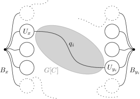
Figure 1: The vertex embedding $B_{x}$ is connected to $B_{y_{i}}$ by the path $q_{i}$ which connects the two branches $U_{x}$ and $U_{y_{i}}$. The dotted branches have an edge embedding adjacent and can thus not be used to connect $B_{y_{i}}$ to $B_{x}$.

If all branches of a vertex embedding $B_{z}$ have either too few neighbors in $C$ or are already adjacent to an edge embedding (i.e., have already been used to embed some other edge), then we want to remove the embedding of $z$. This has to be done in a careful manner in order not to break the invariants. First, move all branches that are not used to connect $z$ to a neighbor to $A$. Note that each such branch $U$ satisfies $|N(U,C)|<\beta|U|$. Next, move the remaining branches along with the adjacent edge embeddings to $A^{\prime}$. Last, the center of $B_{z}$ is moved to $A^{\prime}$ and $z$ is removed from $I$. Note that at most $2(\deg_{H}(z)-1)s$ many vertices are moved to $A^{\prime}$: at most $\deg_{H}(z)-1$ many branches of size $s$ and as many edge embeddings, each again of size at most $s$. On the other hand at least

$$\big{(}r(\deg_{H}(z))-(\deg_{H}(z)-1)\big{)}\cdot s =\deg_{H}(z)\cdot 4s/\beta$$ (20)

many vertices are moved to $A$. Hence the invariant $|A^{\prime}|<\beta|A|/2$ is maintained.

The algorithm terminates the first time either $I=V(H)$ or $|A|\geq n/k$. This completes the description of the algorithm.

It remains to argue that it cannot happen that $|A|\geq n/k$, in other words that when the algorithm terminates, all of $H$ is embedded in $G$. To this end, observe that the size of $\cup_{B\in\mathcal{B}}B$ is upper bounded by

$$s\cdot\left(|E(H)|+\sum_{v\in V(H)}r(\deg_{H}(v))\right) <s\cdot\left(|E(H)|+(4/\beta+1)\sum_{v\in V(H)}\deg_{H}(v)\right)$$

$$\leq s\cdot|E(H)|\cdot\frac{11}{\beta}$$

$$\leq s\cdot\frac{\varepsilon n}{k\log n}\cdot\frac{11}{\beta}$$

$$\leq\beta n/2k\enspace.$$

Furthermore, while $|A|\leq n/k$ we have that

$$|A^{\prime}| <\beta|A|/2\leq\beta n/2k\enspace.$$

Note that this also holds the first time $|A|$ becomes larger than $n/k$. This shows, in particular, that the invariant $|C|\geq n(1-2/k)$ is maintained throughout the execution of the algorithm.

For the sake of contradiction, suppose that the algorithm terminates because of $|A|\geq n/k$. Note that $|N(A)|\leq|A^{\prime}|+\left|\cup_{B\in\mathcal{B}}B\right|+|N(A,C)|<\beta(|A|+n/k)$. We do a case distinction, depending on the size of $A$. In both cases we derive contradiction and thus show that the algorithm only terminates after having embedded all of $H$ into $G$.

1. $n/k\leq|A|\leq n/2$. By expansion and using $\beta<\alpha/3$ we have

   $$\alpha|A|\leq|N(A)|<\beta(|A|+n/k)<\frac{\alpha}{3}(|A|+n/k)\enspace,$$

   which together with $|A|\geq n/k$ yields the desired contradiction.

2. $|A|>n/2$. Note that the first time $|A|\geq n/k$, it also holds that $|A|\leq n(1+1/k)/2$ as the sets added to $A$ are of size at most $|C|/2\leq(n-|A|)/2$. Hence we get that

   $$|N(A)| <\beta\big{(}n/k+|A|\big{)}<\beta n\big{(}1/k+(1+1/k)/2\big{)}\leq\frac{\alpha n}{3(1+\alpha)}\enspace,$$

   using that $k\geq 3$. Note that $N(A)$ is a balanced separator, separating $A$ from $V(G)\setminus A\setminus N(A)$. But this is a contradiction, since Lemma 5.1 states that any balanced separator of $G$ has size at least $\frac{\alpha n}{3(1+\alpha)}$.

5.3 Crosses in Expanders

Let us now turn to the proof of Lemma 5.5, restated here for convenience.

See 5.5

The proof follows a similar algorithm as the proof of Theorem 3.3. In this case we can in fact more or less use the original argument of Krivelevich and Nenadov [44] without any extensions.

Proof 5.7.

The high-level idea of the proof is as follows. First, using the embedding argument of Krivelevich and Nenadov, we find some number $r^{\prime}>r$ pairwise disjoint sets $B_{1},\ldots,B_{r^{\prime}}$ of vertices of $G$ and a final set $C$ disjoint from all $B_{i}$s such that (i) each $B_{i}$ is a connected subgraph of $G$ on $s$ vertices, (ii) the $B_{i}$s have many neighbors in $C$, and (iii) $G[C]$ is expanding. Having these subsets, we can then choose a representative $u_{i}\in N(B_{i},C)$ of each $B_{i}$, take a vertex $v\in C$ of high degree (which exists by the max-degree-robustness of $G$), and apply Lemma 5.3 to find vertex-disjoint paths connecting $N(v)$ to the $u_{i}$s. This establishes the existence of a cross with $v$ as the center and the $B_{i}$s together with the respective paths as branches. See Figure 2 for an illustration.

Let us proceed with the details. In case there is some ambiguity in the verbal description there is also a pseudo code description in Appendix B of what follows.

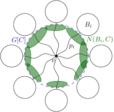
Figure 2: A cross with center $v$ and branches $\{\,V(p_{i})\cup B_{i}\mid i\in[r]\,\}$.

Fix $r$, set $r^{\prime}=r(1+1/\gamma)$ and choose $s\in\mathbb{N}$ maximal such that $s\leq\frac{\gamma n}{k\cdot r^{\prime}}$. Note that $s\geq 1/\gamma$ and if the statement holds for this maximal $s$, then it also holds for smaller values of $s$, as one can always shrink the branches to the appropriate size.

Let us describe an algorithm to identify the sets $\mathcal{B}=\{\,B_{i}\subseteq V(G)\mid i\in[r^{\prime}]\,\}$. The algorithm maintains a partition $A\overset{.}{\cup}\dot{\bigcup}_{B\in\mathcal{B}}B\overset{.}{\cup}C$ of the vertices of $G$. Initially, all sets except $C=V(G)$ are empty. After running the procedure, the set $\mathcal{B}$ contains $r^{\prime}$ pairwise vertex-disjoint sets such that for each $B_{i}\in\mathcal{B}$ it holds that $|B_{i}|=s$ and the induced subgraph $G[B_{i}]$ is a single connected component. Further, for all subfamilies $\mathcal{F}\subseteq\mathcal{B}$ it holds that $\left|\bigcup_{F\in\mathcal{F}}N(F,C)\right|\geq\gamma s|\mathcal{F}|$. Throughout the execution of the algorithm the following invariants are maintained

1. $C$ never increases in size and $|C|\geq n(1-2/k)$,

2. $G[C]$ is a $\gamma$-expander (by restoring expansion whenever needed),

3. $N(A,C)<\beta|A|$, and

4. $\left|\dot{\bigcup}_{B\in\mathcal{B}}B\right|\leq r^{\prime}\cdot s\leq\gamma n/k$.

The algorithm terminates if $\mathcal{B}$ contains $r^{\prime}$ vertex sets as described, or if the size of $A$ reaches $|A|\geq n/k$. The latter case can only occur if there is a small balanced separator in $G$. But $G$ is a $\beta$-expander, so we know from Lemma 5.1 that there are no small balanced separators and hence when the algorithm terminates, $\mathcal{B}$ must contain $r^{\prime}$ sets as described above.

Like in the main algorithm used in the proof of Theorem 3.3, we want to ensure that $G[C]$ is a $\gamma$-expander throughout the algorithm, which is achieved by removing any subset $U\subseteq C$ of size $|U|\leq|C|/2$ with small neighborhood $|N(U,C\setminus U)|<\gamma|U|$ from $C=C\setminus U$ and adding it to $A=A\cup U$.

Repeat the following while there are less than $r^{\prime}$ sets in $\mathcal{B}$. Choose a set of vertices $U\subseteq C$ of size $|U|=s$ such that $G[U]$ is a single connected component. Remove this set from $C=C\setminus U$, add it to $\mathcal{B}=\mathcal{B}\cup\{U\}$ and restore expansion in $G[C]$. After expansion is restored, let $\mathcal{F}\subseteq\mathcal{B}$ be a maximal (possibly empty) family such that $\left|\bigcup_{F\in\mathcal{F}}N(F,C)\right|<\gamma s|\mathcal{F}|$. Remove $\mathcal{F}$ from $\mathcal{B}=\mathcal{B}\setminus\mathcal{F}$, and add these sets to $A=A\cup_{F\in\mathcal{F}}F$.

As mentioned before, the algorithm terminates once there are either $r^{\prime}$ sets in $\mathcal{B}$ or the set $A$ is large $|A|\geq n/k$. This completes the description of the algorithm. Let us argue that the latter cannot happen – for the sake of contradiction, suppose the algorithm terminates because $|A|\geq n/k$. Note that we have $|N(A)|\leq|\cup_{B\in\mathcal{B}}B|+|N(A,C)|<\gamma(|A|+n/k)$. We do a case distincion on the size of $|A|$.

1. $n/k\leq|A|\leq n/2$. By expansion, $\beta|A|\leq N(A)<\gamma(|A|+n/k)<\frac{\beta}{3}(|A|+n/k)$. As $|A|\geq n/k$ this is a contradiction.

2. $|A|\geq n/2$. Note that the first time $|A|\geq n/k$, it also holds that $|A|\leq n(1+1/k)/2$ as the sets added to $A$ are of size at most $|C|/2\leq(n-|A|)/2$. Hence we get (using $k\geq 3$) that

   $$|N(A)| \leq\gamma(n/k+|A|)\leq\gamma n=\frac{\beta n}{3(1+\beta)}.$$

   Note that $N(A)$ is a balanced separator, separating $A$ from $V(G)\setminus A$. But this is a contradiction, since Lemma 5.1 states that any balanced separator of $G$ has size at least $\frac{\beta n}{3(1+\beta)}$.

It remains to obtain an $(r,s)$-cross from the sets $B_{i}$ and the remaining part $C$. Choose a vertex $v\in C$ of degree at least $\deg_{G[C]}(v)\geq r^{\prime}$. Such a vertex $v$ exists, as $|C|\geq(1-2/k)n$ is large (first invariant) and the statement assumes that there is a vertex of degree $r^{\prime}$ in every induced subgraph of size at least $(1-2/k)n$. Let $T$ be a transversal of the family $\{\,N(B,C)\mid B\in\mathcal{B}\,\}$. Note that such a transversal $T$ exists by Hall’s marriage theorem, using that $s\geq 1/\beta$ and that every subset of $\mathcal{B}$ is $\beta$-expanding into $C$.

Apply Lemma 5.3 to $G[C]$ and the vertex sets $N(v)$ and $T$ to conclude that there are pairwise vertex-disjoint paths $\{\,p_{i}\mid i\in[r]\,\}$ each connecting $N(v)$ to a set $N(B_{i},C)$, for some $B_{i}\in\mathcal{B}$. We let the $(r,s)$-cross have center $v$ and branches $\{\,V(p_{i})\cup B_{i}\mid i\in[r]\,\}$. Let us verify that this is indeed a valid $(r,s)$-cross.

Each path $p_{i}$ connects $N(v)$ to $N(B_{i},C)$ and we thus have that, as required, each branch intersects $N(v)$ and that the branches are connected, where we use that the sets $B_{i}\in\mathcal{B}$ are by definition connected. We also need to verify that the branches are pairwise vertex-disjoint. To this end recall that the sets $B_{i}\in\mathcal{B}$ are pairwise disjoint and, furthermore, each such set is disjoint from $C$. As the pairwise vertex-disjoint paths $p_{i}$ live in $G[C]$, these paths do not intersect $\cup_{i\in[r]}B_{i}$ and we may thus conclude that the branches are pairwise vertex-disjoint. Finally, we also need to check that each branch is of size $s$: each set $B_{i}$ is of size $s$ and thus each branch is of size at least $s$. Shrinking the branches to the appropriate size recovers the statement.

5.4 Odd and Even Paths

In this section we prove Lemma 5.6.

See 5.6

The lemma is a corollary of a more general statement about short paths in $\alpha$-expanders. The lemma states that if sets $S,T$, where $|S|\gtrsim|T|/\alpha$, are connected by $|T|$ many short vertex-disjoint paths, then for any large set $U$ there is again a set of short vertex-disjoint paths that does not only connect every vertex of $T$ to $S$ but also a vertex from $U$ to $S$.

In order to state the lemma, let us introduce some notation. For a graph $G$ and vertex sets $S,T\subseteq V(G)$, denote by $L^{{G}}_{\text{disj}}(T,S)$ the minimum total length of connecting all vertices of $T$ to $S$ by pairwise vertex-disjoint paths;

$$L^{{G}}_{\text{disj}}(T,S) =\min_{\{\,p_{t}\mid t\in T\,\}}\sum_{t\in T}|p_{t}|$$ (21)

where $\{\,p_{t}\mid t\in T\,\}$ ranges over all sets of pairwise vertex-disjoint paths such that $p_{t}$ connects $t$ to $S$ (note the paths $\{p_{t}\}$ are not allowed to intersect even in $S$). If no such set of paths exists, the value of the minimum is taken to be $\infty$. If the graph $G$ is clear from context, we omit the superscript.

A similar lemma (though without the essential upper bound on the path lengths) has appeared in e.g. [26].

Lemma 5.8.

Let $G$ be a $\beta$-expander on $n$ vertices and $S,T\subseteq V(G)$ satisfy $|S|\geq|T|(1+2/\beta)$. Then every set $U\subseteq V(G)$, of size $|U|\geq(L_{\text{disj}}(T,S)+|T|)(1+2/\beta)$, contains a vertex $u\in U$ such that $L_{\text{disj}}(T\cup\{u\},S)\leq 7(L_{\text{disj}}(T,S)+|T|)/\beta+2D^{\text{{\o}}}_{{\beta/2}}\log n$.

Lemma 5.6 follows by a single application of Lemma 5.8.

Proof 5.9 (Proof of Lemma 5.6).

Let $C$ denote an odd cycle of length $\ell\geq 1+2/\beta$, as guaranteed to exist, and denote by $p$ a shortest path connecting $u$ to $C$. By Lemma 2.4, we know that $|p|\leq D^{\text{{\o}}}_{{\beta}}\log n$. Apply Lemma 5.8 to $S=C$, $T=\{u\}$, $p_{u}=p$, and $U=A$. We conclude that there is a $v\in A$ and two vertex-disjoint paths $p_{u}^{\prime},p_{v}^{\prime}$ connecting $u$ and $v$ to $C$, of total length at most $(15D^{\text{{\o}}}_{{\beta/2}}/\beta)\log n$. We can join these paths into a path between $u$ and $v$ by walking along $C$ in either of the two directions. Since $C$ has odd length this results in one odd and one even length path connecting $u$ to $v$, each of length at most $\ell+(15D^{\text{{\o}}}_{{\beta/2}}/\beta)\log n$, as required.

Proof 5.10 (Proof of Lemma 5.8).

Denote by $\mathcal{P}=\{\,p_{t}\mid t\in T\,\}$ a set of pairwise vertex-disjoint paths of smallest total length, where the path $p_{t}$ connects $t$ to $S$. Let $V(\mathcal{P})=\cup_{p\in\mathcal{P}}V(p)$ denote all the vertices in the paths in $\mathcal{P}$. Clearly, $|V(\mathcal{P})|=L_{\text{disj}}(T,S)+|T|$. Set $m=|V(\mathcal{P})|(1+2/\beta)$ and $r=\lceil\frac{\log m}{\log(1+\beta/2)}\rceil$. Note that $n\geq|U|\geq m$ and hence $r\leq\frac{1}{2}D^{\text{{\o}}}_{{\beta/2}}\log n$.

If $|S|\geq m$, apply Corollary 2.7 to $V(\mathcal{P})$, $S\setminus V(\mathcal{P})$ and $U\setminus V(\mathcal{P})$ to conclude that there is a path $p$ of length $D^{\text{{\o}}}_{{\beta/2}}\log n$ connecting $S\setminus V(\mathcal{P})$ to $U\setminus V(\mathcal{P})$ in $G\setminus V(\mathcal{P})$. The set $\mathcal{P}\cup\{p\}$ clearly satisfies the conclusion of the lemma.

Otherwise, if $|S|<m$, we want to get into a position where we can again apply Corollary 2.7. To this end, we define a sequence of sets of vertices $S=S_{0}\subseteq S_{1}\subseteq\ldots\subseteq S_{\ell}\subseteq V(G)$ that are in some sense well-connected to $S$. We formalize this property after explaining how to obtain these sets.

The set $S_{i+1}$ is defined in terms of $S_{i}$ using the following process. Let $w^{i}_{t}$ be the last vertex on the path $p_{t}$ (viewed as a path from $S$ to $t$) that is in $S_{i}$ and $W_{i}=\{\,w^{i}_{t}\mid t\in T\,\}$. Suppose $|S_{i}|<m$ and there is a path of length at most $r$ connecting $S_{i}\setminus W_{i}$ to $V(\mathcal{P})\setminus S_{i}$ in the graph $G\setminus W_{i}$ . Denote by $q_{i}$ a minimal such path, denote by $w$ the endpoint of $q_{i}$ in $V(\mathcal{P})\setminus S_{i}$, and let $t_{i}\in T$ be such that $w\in V(p_{t_{i}})$. Then, define $S_{i+1}=S_{i}\cup q_{i}\cup p_{t_{i}}[w^{t_{i}}_{i},w]$. Otherwise, if $|S_{i}|\geq m$ or there is no such $q_{i}$, set $\ell=i$ and stop the process. There is an illustration of this process in Figure 3.

The following claim formalizes the well-connectedness property of $S_{\ell}$.

Claim 11.

For every vertex $s^{\star}\in S_{\ell}\setminus W_{\ell}$ it holds that $L^{{G[S_{\ell}\cup V(\mathcal{P})]}}_{\text{disj}}(T\cup\{s^{\star}\},S)\leq L^{{G}}_{\text{disj}}(T,S)+|S_{\ell}|$ and furthermore the paths achieving this bound are the same as the paths in $\mathcal{P}$ outside $S_{\ell}\setminus W_{\ell}$.

Proof 5.11.

Proof by induction on $i\in\{0,\ldots,\ell\}$. The base case $i=0$ clearly holds – we have for all $s^{\star}\in S_{0}\setminus W_{0}\subseteq S$ that $L^{{G[S_{0}\cup V(\mathcal{P})]}}_{\text{disj}}(T\cup\{s^{\star}\},S)=L^{{G}}_{\text{disj}}(T,S)$.

Suppose the statement is true for some $i\in\{0,\ldots\ell-1\}$ and let us prove that is then true for $i+1$ as well. By the inductive hypothesis, $L^{{G[S_{i}\cup V(\mathcal{P})]}}_{\text{disj}}(T\cup\{s_{i}\},S)\leq L^{{G}}_{\text{disj}}(T,S)+|S_{i}|$, and this bound can be achieved by a set of paths $\mathcal{P}^{\prime}$ which follow $\mathcal{P}$ outside $S_{i}\setminus W_{i}$.

Fix an arbitrary $s^{\star}\in S_{i+1}\setminus W_{i+1}$. By the induction hypothesis the claim holds for $s^{\star}\in S_{i}\setminus W_{i}$, so we may assume that either $s^{\star}\in q_{i}$, or $s^{\star}\in p_{t_{i}}[w^{t_{i}}_{i},w^{t_{i}}_{i+1}]$. If $s^{\star}\in q_{i}$ (excluding its endpoint $w^{t_{i}}_{i+1}$) then we simply extend the path in $\mathcal{P}^{\prime}$ ending in $s_{i}$ with the subpath of $q_{i}$ from $s^{\star}$ to $s_{i}$, increasing the total length of $\mathcal{P}^{\prime}$ by at most $|q_{i}|$. On the other hand if $s^{\star}\in p_{t_{i}}[w^{t_{i}}_{i},w^{t_{i}}_{i+1}]$ then we reroute the path from $t_{i}$ in $\mathcal{P}^{\prime}$ to $s_{i}$ via $q_{i}$ and then use the now unused part of $p_{t_{i}}$ to connect $s^{\star}$ to $S$, again increasing the total length of $\mathcal{P}^{\prime}$ by at most $|q_{i}|$. There is an illustration of the two cases in Figure 3.

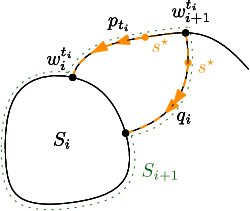
(a)

(b)

(c)

Figure 3: Given the set $S_{i}$, the first figure depicts the process of obtaining the set $S_{i+1}$. The following figures indicate how to route the paths, as in the proof of Claim 11, depending on where $s^{\star}$ is located.

In either case, we can connect $T$ and $s^{\star}$ to $S$ via vertex-disjoint paths of length at most

$$L^{{G[S_{i+1}\cup V(\mathcal{P})]}}_{\text{disj}}(T\cup\{s^{\star}\},S)\leq L^{{G}}_{\text{disj}}(T,S)+|S_{i}|+|q_{i}|\leq L^{{G}}_{\text{disj}}(T,S)+|S_{i+1}|,$$

as desired.

It is easy to see that $|S_{\ell}|\leq 2m+r$: the number of vertices added by $p_{t_{i}}[w^{t_{i}}_{i},w^{t_{i}}_{i+1}]$ is always upper bounded by $|V(\mathcal{P})|\leq m$. Suppose there is a path $p^{\star}$ of length $|p^{\star}|\leq D^{\text{{\o}}}_{{\beta/2}}\log n+r$ connecting some vertex $s^{\star}\in S_{\ell}\setminus W_{\ell}$ to $u^{\star}\in U\setminus V(\mathcal{P}_{\ell})$ in $G\setminus V(\mathcal{P}_{\ell})$. We can then “compose” the paths to conclude that

$$L^{{G}}_{\text{disj}}(T\cup\{u^{\star}\},S) \leq L^{{G[S_{\ell}]}}_{\text{disj}}(W_{\ell}\cup\{s^{\star}\},S)+L^{{G\setminus(S_{\ell}\setminus(W_{\ell}\cup\{s^{\star}\}))}}_{\text{disj}}(W_{\ell}\cup\{s^{\star}\},T\cup\{u^{\star}\})$$ (22)

$$\leq|S_{\ell}|+L^{{G}}_{\text{disj}}(T,S)+|p^{\star}|$$ (23)

$$\leq|S_{\ell}|+L^{{G}}_{\text{disj}}(T,S)+D^{\text{{\o}}}_{{\beta/2}}\log n+r$$ (24)

$$\leq 2m+r+L^{{G}}_{\text{disj}}(T,S)+D^{\text{{\o}}}_{{\beta/2}}\log n+r$$ (25)

$$\leq 7(L^{{G}}_{\text{disj}}(T,S)+|T|)/\beta+2D^{\text{{\o}}}_{{\beta/2}}\log n\enspace,$$ (26)

as claimed in the statement.

It remains to establish that such a path $p^{\star}$ exists. If $|S_{\ell}|\geq m$, apply Corollary 2.7 to $V(\mathcal{P})$, $S_{\ell}\setminus W_{\ell}$ and $U\setminus V(\mathcal{P})$ to conclude that there is a path $p^{\star}$ of length at most $|p^{\star}|\leq D^{\text{{\o}}}_{{\beta/2}}\log n$ that connects $S_{\ell}\setminus W_{\ell}$ to $U\setminus V(\mathcal{P})$ in $G\setminus V(\mathcal{P})$.

Otherwise, by construction, $S_{\ell}\setminus W_{\ell}$ cannot reach $V(\mathcal{P})\setminus W_{\ell}$ within $r$ steps in $G\setminus W_{\ell}$. Hence, to argue that in $G\setminus V(\mathcal{P})$ the ball of radius $r$ around $S_{\ell}\setminus W_{\ell}$ is large, we do not need to apply Lemma 2.5 to $V(\mathcal{P})$ and $S_{\ell}\setminus W_{\ell}$ but in fact can apply it to $W_{\ell}$ and $S_{\ell}\setminus W_{\ell}$, where we use that $|S_{\ell}\setminus W_{\ell}|\geq|S|-|T|\geq 2|T|/\beta$. This enables us to grow $S_{\ell}\setminus W_{\ell}$ into a set $S^{\star}=B_{r}^{G\setminus W_{\ell}}(S_{\ell}\setminus W_{\ell})=B_{r}^{G\setminus V(\mathcal{P})}(S_{\ell}\setminus W_{\ell})$ of size at least $m$. Now we are in a position to apply Corollary 2.7 to $V(\mathcal{P})$, $S^{\star}$ and $U\setminus V(\mathcal{P})$ to conclude that there is a path of length at most $D^{\text{{\o}}}_{{\beta/2}}\log n$ that connects $S^{\star}$ to $U\setminus V(\mathcal{P})$ in $G\setminus V(\mathcal{P})$. Taking an additional $r$ steps in $G[S^{\star}]$, one can reach $S_{\ell}\setminus W_{\ell}$, as required. This concludes the proof of the lemma.

6 Concluding Remarks

We have established average-case lower bounds for refuting the perfect matching formula and more generally the $\operatorname{Card}(G,\vec{t})$ formula in random $d$-regular graphs on an odd number of vertices. Let us conclude by discussing some further loose ends and mention some open problems.

6.1 Polynomial Calculus Space Lower Bounds

The space of a PC refutation $\pi$ is the amount of memory needed to verify $\pi$. The PC space of a formula $\mathcal{F}$ is then the minimum space required for any PC refutation $\pi$ of $\mathcal{F}$. As this is rather tangential to the rest of the paper we refer to [24] for formal definitions. For convenience, let us restate our result on PC space.

See 1.3

The proof idea is to take the worst-case Tseitin lower bounds from Filmus et al. [24] for which PC requires $\Omega(n)$ space and embed these into a vertex expander of large enough average degree. The only compication that arises is that these formulas are defined over multigraphs – the multigraph $H$ is obtained from an appropriate constant degree graph $G$ by doubling each edge. An inspection of the proof of Theorem 3.3 reveals that $H$ may be a multigraph and we can thus implement our proof strategy.

Proof 6.1 (Proof Sketch).

Consider the worst-case instance $H$ from Filmus et al. [24] on $\varepsilon n/\log n$ vertices, for some small enough $\varepsilon>0$. Apply Theorem 3.3 to $H$ and $G$. This gives a topological embedding of $H$ in $G$, with no control of the parities of the length of the paths. Consider a restriction $\rho$ that sets the variables outside the embedding of $H$ such that no axiom is falsified (see, e.g., [54]). By appropriately substituting the variables on each path of the topological embedding we obtain that the worst-case instance $\tau(H)$ is an affine restriction of $\tau(G)$. As an affine restriction only reduces the amount of space needed to verify a proof, we see that $\tau(G)$ requires PC space $\Omega(n/\log n)$.

6.2 Paths in Expanders

The arguments used in the proof of Theorem 3.3 can be adapted to make partial progress on a question by Friedman and Krivelevich [26]. They asked, given a positive integer $q$, whether it is possible to guarantee the existence of a cycle whose length is divisible by $q$ in every $\alpha$-expander.

We can show that for all primes $q$ satisfying $1/\poly(\alpha)\ll q\ll\sqrt{n/\log n}$, this indeed holds. In fact, for all $a\in\mathbb{Z}_{q}$, we can show that there is a cycle of length $a\bmod q$.

The idea is to embed a cycle $C_{q^{2}}$ of length $q^{2}$ into $G$ such that between any two vertices there are two paths whose length difference is non-zero modulo $q$. If we can ensure this, as all $0\neq b\in\mathbb{Z}_{q}$ are generators, we can choose one path between all embedded vertices such that the length of the cycle is $a\bmod q$ for any $a\in\mathbb{Z}_{q}$.

In order to obtain paths of different length modulo $q$, let us embed a cycle $c_{e}$ (of length $\gg 1/\poly(\alpha)$) for each edge $e=\{u,v\}$. We then want to connect the vertex embeddings $B_{u},B_{v}$ to $c_{e}$ such that the two resulting paths are of different length modulo $q$. Note that once a vertex is connected to the cycle, there are only about $2/q$ vertices in $c_{e}$ such that both paths are of equal length modulo $q$. As $q$ is rather large and thus there are few such “bad” vertices, when an edge embedding has to be moved to the sets $A,A^{\prime}$, we can ensure that the set $A^{\prime}$ remains relatively small compared to $A$.

6.3 Open Problems

The main concrete problem left open is to reduce the degree of the hard graphs: the embedding approach taken in the worst-case to average-case reduction results in very large degree $d$; while Theorem 1.1 does not give an explicit estimate on $d_{0}$ one can trace through the proofs and get an estimate of around $15\,000$. The main bottleneck that prevents us from reducing this is the Partition Lemma and in particular the dependence of $d_{0}$ on $c$ and $\epsilon$ in Lemma 4.3. If this part could be significantly improved or circumvented we believe that the degree of the graph could be significantly reduced, although it would still be relatively large (at least a few hundreds). It would be interesting to see what happens for very small degrees, e.g., $4$-regular graph (recall that since $n$ is odd, $d$ must be even) – is $\mathsf{PM}(G)$ hard with high probability even for these graphs?

Another interesting question is the proof complexity of perfect matching in Polynomial Calculus over $\mathbb{F}_{2}$ (or any other field of characteristic $2$). While PC${}_{\mathbb{F}_{2}}$ can refute the perfect matching formula on an odd number of vertices for parity reasons, the situation is less clear when the number of vertices is even. Are there graphs $G$ that do not admit perfect matchings but PC${}_{\mathbb{F}_{2}}$ requires exponential size refutations?

We establish Theorem 1.1 for random graphs and not for all spectral expanders. Our proof mostly uses the expansion properties of random graphs, except for two places: in the Partition Lemma to argue that every subgraph contains a not too short odd cycle, and for the contiguity argument in Section 3.2. However, we believe that it should be possible to circumvent these uses of randomness and establish the lower bounds for all spectral expanders.

Theorem 1.1 only gives lower bounds for $\operatorname{Card}(G,b)$ when $b=\vec{t}$ is a constant vector (and $G$ is regular). It would be nice to characterize more generally for which vectors $b$ the formula is hard. In the analogous setting for Tseitin formulas, the precise charges of the vertices do not matter, as long as the sum of charges is odd the formula remains hard to refute on a random graph [15, 32]. In the $\operatorname{Card}(G,b)$ case however this is not the case. For instance, if the vector of target degrees $b$ violates any of the inequalities of the Erdős-Gallai characterization of degree sequences then SoS (in fact even Sherali-Adams) can easily refute $\operatorname{Card}(G,b)$.

In the case when $G$ is the complete graph this in fact gives a complete characterization of the easy and hard vectors $b$ but for sparse graphs the situation is less clear. Is there a nice characterization of vectors $b$ for which $\operatorname{Card}(G,b)$ is hard for SoS with high probability over a random $d$-regular $G$?

More broadly, another open problem is to prove SoS lower bounds for random CSPs that do not support pairwise uniform distributions (cf. the brief discussion on CSPs in Section 1.2). Viewed this way, our results establish hardness of random monotone $1$-in-$k$-SAT instances with two occurrences per variable, for some large constant $k$. Reducing $k$ corresponds to the aforementioned problem of reducing the degree, but some other natural questions are to look at other CSPs such as $1$-in-$k$-SAT with negated literals, or to understand the hardness as a function of the density of the instances.

Acknowledgements.

The authors are grateful to Susanna de Rezende, Johan Håstad, Jakob Nordström, Dmitry Sokolov and Aleksa Stanković for helpful discussions. In particular we would like to thank Jakob Nordström who suggested to consider the even coloring formula and brought the problem about Polynomial Calculus space to our attention. Finally we would like to thank the anonymous conference and jounral referees for their very detailed reviews and many helpful remarks.

Appendix A Worst-Case Lower Bounds

In this section we describe a general reduction from the Tseitin formula to the Perfect Matching formula as it appeared in [15] for Polynomial Calculus. We then observe that this reduction also works for the SoS and bounded depth Frege proof systems.

Starting from a graph $G$ such that the Tseitin formula $\tau(G)$ is hard for a proof system $P$, we want to craft a graph $H$ so that $\mathsf{PM}(H)$ is hard for $P$. To simplify the presentation, let us assume that $G$ is $d$-regular. As we are interested in unsatisfiable instances, i.e., when $G$ has an odd number of vertices, we may assume that $d$ is even.

The graph $H$ is a “blow-up” (or “lift”) of $G$: each vertex in $V(G)$ is lifted to a clique of $d+1$ vertices and each lifted edge connects a single pair of vertices from the corresponding cliques. If we denote the lifted vertices of $v\in V(G)$ by $\mathsf{lift}(v)=\{(v,\star),(v,1),\ldots,(v,d)\}$, we add for each edge $\{u,v\}\in E(G)$, where $v$ is the $i$th neighbor of $u$ and $u$ is the $j$th neighbor of $v$, an edge $\{(u,i),(v,j)\}$. An illustration of the construction of $H$ can be found in Figure 4.

(a) The graph $G$.

(b) The lift of a single vertex.

(c) The lifted graph $H$.

Figure 4: An illustration of the blow-up construction, starting from a 4-regular graph.

For intuition, let us describe how we would obtain a satisfying assignment to the Perfect Matching Formula from a hypothetical satisfying assignment to the Tseitin Formula. Set the lifted edges to the same value as they are set to in the Tseitin Formula. Now observe that each charge is odd and hence there is an even number of vertices left that are not matched yet in each $\mathsf{lift}(v)$, for $v\in V(G)$. As the vertices in $\mathsf{lift}(v)$ form a clique, we can select a perfect matching on these unmatched vertices to obtain a satisfying assignment to the Perfect Matching Formula.

Buss et al. [15] showed that Polynomial Calculus can simulate this reduction.

Theorem A.1 ([15]).

There are graphs $G$ on an odd number of vertices $n$ and maximum degree $\Delta(G)=5$ such that Polynomial Calculus over any field of characteristic different from $2$ requires degree $\Theta(n)$ to refute $\mathsf{PM}(G)$.

What remains is to check that this reduction also gives Perfect Matching worst-case lower bounds for Sum-of-Squares and bounded depth Frege. This straightforward verification is carried out in the following two sections.

A.1 Sum-of-Squares

A nice property of the Sum-of-Squares system is that if the variables for a formula $\mathcal{Q}$ can be expressed as well-behaved low-degree polynomials in the variables of another formula $\mathcal{P}$ for which a pseudo-expectation exists, then a pseudo-expectation also exists for $\mathcal{Q}$. This property is well-known but let us state and quickly prove the exact version we need.

Claim 12.

Let $\mathcal{P}\subseteq\mathbb{R}[x_{1},\ldots,x_{n}]$ and $\mathcal{Q}\subseteq\mathbb{R}[y_{1},\ldots,y_{m}]$ be two systems of polynomial equations. Let $\tilde{\mathbb{E}}_{\mathcal{Q}}$ be a degree $D$ pseudo-expectation for $\mathcal{Q}$. Suppose there is a function $f:\{x_{1},\ldots,x_{m}\}\to\mathbb{R}[y_{1},\ldots y_{n}]$, mapping the $x$ variables to polynomials in $y$ of degree at most $t$. Extend $f$ to polynomials by applying the function to each variable individually. If $f$ satisfies that $\tilde{\mathbb{E}}_{\mathcal{Q}}[f(r\cdot p)]=0$, for all $p\in\mathcal{P}$ and $r\in\mathbb{R}[x_{1},\ldots x_{m}]$ of degree $\deg(r\cdot p)\leq D/t$, then $\tilde{\mathbb{E}}_{\mathcal{Q}}\circ f$ is a degree $D/t$ pseudo-expectation for $\mathcal{P}$.

Proof A.2.

As $f$ only maps variables we have that $\tilde{\mathbb{E}}_{\mathcal{Q}}[f(1)]=\tilde{\mathbb{E}}_{\mathcal{Q}}[1]=1$. Also, we need to check that $\tilde{\mathbb{E}}_{\mathcal{Q}}[f(s^{2})]\geq 0$ for $s\in\mathbb{R}[x_{1},\ldots,x_{m}]$ of degree $\deg(s)\leq D/2t$. As we apply $f$ individually to each variable, we can write $\tilde{\mathbb{E}}_{\mathcal{Q}}[f(s^{2})]=\tilde{\mathbb{E}}_{\mathcal{Q}}[\big{(}\sum_{t\in s}f(t)\big{)}^{2}]\geq 0$, as $\tilde{\mathbb{E}}_{\mathcal{Q}}$ is a degree $D$ pseudo-expectation.

In order to apply Claim 12 with $\mathcal{Q}=\tau(G)$ and $\mathcal{P}=\mathsf{PM}(H)$, we need to express each variable from the Perfect Matching formula as a low degree polynomial in the Tseitin variables.

Let us recall some notation. For a vertex $v\in V(G)$, let $Y_{v}$ be the set of Tseitin variables corresponding to edges incident to $v$ and denote by $A_{v}$ all boolean assignments to $Y_{v}$ that satisfy the vertex axiom of $v$, i.e., assignments that set an odd number of edges to true. For a Tseitin variable $y_{e}$, where $e\in E(G)$, let $\mathsf{lift}(y_{e})\in E(H)$ denote the lifted edge variable.

With this notation at hand, let us define the function $f$ to use in Claim 12. Variables that correspond to lifted edges, $x_{e}=\mathsf{lift}(y_{e^{\prime}})$ for some $e^{\prime}\in E(G)$, are set to 1 if and only if $y_{e^{\prime}}$ is set to $1$ and the variables in $Y_{v}$ are set according to some assignment in $A_{v}$:

$$f(x_{e})=\sum_{\begin{subarray}{c}\alpha\in A_{v}\\ \alpha(y_{e^{\prime}})=1\end{subarray}}\mathbbm{1}_{\{Y_{v}=\alpha\}}\enspace.$$ (27)

Note that this is a polynomial of degree $\deg(v)=d$ in the $y_{e}$’s. For each assignment $\alpha\in A_{v}$, set the variables in $\mathsf{lift}(Y_{v})$ according to $\alpha$ and fix a matching $m_{\alpha}$ on the vertices in $\mathsf{lift}(v)$ not matched by $\alpha$. For any edge $e\subseteq\mathsf{lift}(v)$, let

$$f(x_{e})=\sum_{\begin{subarray}{c}\alpha\in A_{v}\\ e\in m_{\alpha}\end{subarray}}\mathbbm{1}_{\{Y_{v}=\alpha\}}\enspace.$$ (28)

If we apply $f$ individually to each variable, we claim that for $i\in\{1,\ldots,d\}$ and $v\in V(G)$ the polynomial $f(q^{\mathsf{PM}}_{(v,i)})$ is equal to the Tseitin axiom $q^{\tau}_{v}$:

$$f(q^{\mathsf{PM}}_{(v,i)}) =\sum_{e\ni(v,i)}f(x_{e})-1$$ (29)

$$=\sum_{\begin{subarray}{c}\alpha\in A_{v}\\ \alpha(y_{e^{\prime}})=1\end{subarray}}\mathbbm{1}_{\{Y_{v}=\alpha\}}+\sum_{\begin{subarray}{c}\alpha\in A_{v}\\ \alpha(y_{e^{\prime}})=0\end{subarray}}\mathbbm{1}_{\{Y_{v}=\alpha\}}-1$$ (30)

$$=q^{\tau}_{v}\enspace,$$ (31)

using that the $m_{\alpha}$ are matchings. The axioms $q^{\mathsf{PM}}_{(v,\star)}$ are handled similarly:

$$f(q^{\mathsf{PM}}_{(v,\star)})=\sum_{e\ni(v,\star)}f(x_{e})-1=\sum_{\begin{subarray}{c}\alpha\in A_{v}\end{subarray}}\mathbbm{1}_{\{Y_{v}=\alpha\}}-1=q^{\tau}_{v}\enspace.$$ (32)

As $\tilde{\mathbb{E}}_{\tau(G)}$ maps all axioms multiplied by a low degree polynomial to 0, the same holds for $\tilde{\mathbb{E}}_{\tau(G)}\circ f$ and we can thus apply Claim 12.

We conclude that if there is a degree $D$ pseudo-expectation $\tilde{\mathbb{E}}_{\tau(G)}$ for the Tseitin Formula $\tau(G)$, then there is a degree $D/d$ pseudo-expectation $\tilde{\mathbb{E}}_{\mathsf{PM}(H)}$ for the Perfect Matching formula over the lifted graph $H$. Using Grigoriev’s Tseitin lower bound [32] we obtain the following Theorem.

Theorem A.3.

There are graphs $G$ on an odd number of vertices $n$ and maximum degree $\Delta(G)=5$ for which SoS requires degree $\Theta(n)$ to refute $\mathsf{PM}(G)$.

A.2 Bounded Depth Frege

In this section we intend to prove the following theorem.

Theorem A.4.

There is a constant $c>0$ such that the following holds. Suppose $D\leq\frac{c\log n}{\log\log n}$. Then there are graphs $G$ on an odd number of vertices $n$ and maximum degree $\Delta(G)=5$ such that any depth-$D$ Frege refutation of $\mathsf{PM}(G)$ requires size $\exp(\Omega(n^{c/D}))$.

As in the previous section we use a function $f$, mapping Perfect Matching variables to low depth formulas in the Tseitin Variables, to argue that we can transform a refutation of $\mathsf{PM}(H)$ into a refutation of the Tseitin formula $\tau(G)$. Assuming that this can be done, we use the following recent result of Håstad about the Tseitin formula over the grid to obtain Theorem A.4.

Theorem A.5 ([34]).

Suppose that $D\leq\frac{\log n}{59\log\log n}$, then any depth-$D$ Frege refutation of the Tseitin formula on the $n\times n$ grid requires size $\exp(\Omega(n^{1/58(D+1)}))$.

In the previous section $f$ mapped to polynomials. As we are now working with formulas we need to translate the polynomials to formulas. This is straightforward; reusing notation from the previous section, let

$$f(x_{e})=\bigvee_{\begin{subarray}{c}\alpha\in A_{v}\\ \alpha(y_{e^{\prime}})=1\end{subarray}}\mathbbm{1}_{\{Y_{v}=\alpha\}}\enspace,$$ (33)

if $x_{e}=\mathsf{lift}(y_{e^{\prime}})$ is a lifted edge. Else let

$$f(x_{e})=\bigvee_{\begin{subarray}{c}\alpha\in A_{v}\\ e\in m_{\alpha}\end{subarray}}\mathbbm{1}_{\{Y_{v}=\alpha\}}\enspace.$$ (34)

Suppose there is a depth-$D$ Frege refutation $\pi$ of the Perfect Matching formula $\mathsf{PM}(H)$. Replace each occurrence of a Perfect Matching variable $x_{e}$ by $f(x_{e})$ to obtain a depth-$(D+2)$ refutation $\pi^{\prime}$. We claim that $\pi^{\prime}$ can be massaged into a refutation of the Tseitin formula $\tau(G)$ of size $O_{d}(\operatorname{\sf{Size}}(\pi))$.

To this end we need to argue that $f$ maps Perfect Matching axioms to Tseitin Axioms or tautologies that are derivable in small size and depth. Analoguous to SoS observe that for all $v\in V(G)$ and $i\in\{1,\ldots,d\}$,

$$f(\bigvee_{e\ni(v,i)}x_{e}) =\bigvee_{e\ni(v,i)}f(x_{e})$$ (35)

$$=\bigvee_{\begin{subarray}{c}\alpha\in A_{v}\\ \alpha(y_{e^{\prime}})=1\end{subarray}}\mathbbm{1}_{\{Y_{v}=\alpha\}}\vee\bigvee_{\begin{subarray}{c}\alpha\in A_{v}\\ \alpha(y_{e^{\prime}})=0\end{subarray}}\mathbbm{1}_{\{Y_{v}=\alpha\}}\enspace.$$ (36)

Note that that the final formula is equal to the axiom $q^{\tau}_{v}$, up to a reordering of the terms. As the axioms are over $d$ variables, which is constant in our case, this formula can be derived from $q^{\tau}_{v}$ in constant depth and size. The axiom for the vertex $(v,\star)$ is handled in a similar manner.

Last we need to show that the axioms $\bar{x}_{e}\vee\bar{x}_{e^{\prime}}$, for edges $e\neq e^{\prime}\in E(H)$ satisfying $e\cap e^{\prime}\neq\emptyset$, are mapped to a tautology derivable in small size and depth. If we let $\{(v,i)\}=e\cap e^{\prime}$ we can write

$$f(\bar{x}_{e}\vee\bar{x}_{e^{\prime}})=\big{(}\lnot\bigvee_{\beta\in B}\mathbbm{1}_{\{Y_{v}=\beta\}}\big{)}\vee\big{(}\lnot\bigvee_{\gamma\in C}\mathbbm{1}_{\{Y_{v}=\gamma\}}\big{)}\enspace,$$ (37)

for disjoint subsets $B,C\subseteq A_{v}$. Observe that this formula is a tautology and defined on $d$ variables. Thus it is derivable in constant depth and size dependent on $d$, which is constant in our case.

Appendix B Embedding Algorithm

1 $\textnormal{{FixExpansion}}(G,C,A,\beta)$ while $G[C]$ is not a $\beta$-expander do

2         $U\leftarrow_{\text{any}}$ subset of $C$ such that $|U|\leq|C|/2$ and $|N(U,C\setminus U)|<\beta|U|$ ;

3         $C\leftarrow C\setminus U$ ;

4         $A\leftarrow A\cup U$

Algorithm 1 Restores $\beta$-expansion of $G[C]$.

Require : Conditions of Lemma 5.5.

1

2$\textnormal{{EmbedVertex}}(G,r,s,\beta,k)$

3$\gamma\leftarrow\frac{\beta}{3(1+\beta)}$ ;

4 $s\leftarrow\max\{1/\gamma,s\}$ ;

5 $r^{\prime}\leftarrow(1+1/\gamma)r$ ;

6 $A,\mathcal{B}\leftarrow\emptyset;C\leftarrow V(G)$ ;

7

8while $|\mathcal{B}|<r^{\prime}$ do

9         $U\leftarrow_{\text{any}}$ subset of $C$ such that $|U|=s$ and $G[U]$ is a single connected component ;

10         $\mathcal{B}\leftarrow\mathcal{B}\cup\{U\}$; $C\leftarrow C\setminus U$ ;

11         $\textnormal{{FixExpansion}}(G,C,A,\gamma)$ ;

12        

13        $\mathcal{F}\subseteq\mathcal{B}$ maximal such that $|\cup_{F\in\mathcal{F}}N(F,C)|<\gamma s|\mathcal{F}|$ ;

14         $\mathcal{B}\leftarrow\mathcal{B}\setminus\mathcal{F}$; $A\leftarrow A\cup_{F\in\mathcal{F}}F$ ;

15        

16         $v\leftarrow_{\text{any}}C$ such that $\deg_{G[C]}(v)\geq r^{\prime}$ ;

17         $F\leftarrow$ a transversal of $\{\,N(B,C)\mid B\in\mathcal{B}\,\}$ ;

18         $\{\,p_{i}\mid i\in[r]\,\}\leftarrow$ from Lemma 5.3 applied to $G[C]$, $v$ and $F$ ;

         return $\{v\}\cup\{\,V(p_{i})\cup B_{i}\mid i\in[r]\,\}$ ;

          $\triangleright$  Shrink branches appropriately

Algorithm 2 Finds an $(r,s)$-cross in an $\beta$-expander $G$ as in the proof of Lemma 5.5.

$\textnormal{{UnEmbedVertex}}(A,A^{\prime},B,H,I,x)$ $(v,\mathcal{U})\leftarrow B_{x}$ ;

  $\triangleright$  $v$ is the center and $\mathcal{U}$ are the branches of $B_{x}$

1 $B\leftarrow B\setminus B_{x}$; $I\leftarrow I\setminus x$ ;

2 $W\leftarrow\emptyset$ ;

3

4for all $e\in E(H)$ such that $x\in e$ and $e$ is embedded do

5         let $U\leftarrow\mathcal{U}$ be the branch adjacent to $B_{e}$ ;

6         $\mathcal{U}\leftarrow\mathcal{U}\setminus U$ ;

7         $B\leftarrow B\setminus B_{e}$ ;

8         $W\leftarrow W\cup U\cup B_{e}$ ;

9        

         $A\leftarrow A\cup\mathcal{U}$ ;

          $\triangleright$  First add to $A$, then to $A^{\prime}$ to maintain the invariant

10         $A^{\prime}\leftarrow A^{\prime}\cup W\cup\{v\}$ ;

Algorithm 3 Remove the embedding of vertex $x$.

1 $\textnormal{{EmbedGraph}}(H,G,\alpha)$ $\beta\leftarrow\alpha/3(1+\alpha)$ ;

2 $A,A^{\prime},B\leftarrow\emptyset;C\leftarrow V(G)$ ;

3 $I\leftarrow\emptyset$ ;

4

5while $I\neq V(H)$ do

6         $x\leftarrow_{\text{any}}V(H)\setminus I$ ;

7         $B_{x}\leftarrow\textnormal{{EmbedVertex}}(G[C],\deg_{H}(x),s,\beta,k)$ ;

8         $C\leftarrow C\setminus B_{x}$; $B\leftarrow B\cup B_{x}$; $I\leftarrow I\cup x$ ;

9         $\textnormal{{FixExpansion}}(G,C,A,\beta)$ ;

10         $\mathcal{U}_{\text{free}}(K)\leftarrow$ branches of the cross $K$ that are not used to connect to a neighbor ;

11        

12        for all $\{x,y\}\in E(H)$ such that $y\in I$ do

13                 Try;

14                   $U_{z}\leftarrow_{\text{any}}\mathcal{U}_{\text{free}}(B_{z})$ such that $|N(U_{z},C)|\geq\beta|U_{z}|$ for $z\in\{x,y\}$ ;

15                 Catch no such $U_{z}$ for $z\in\{x,y\}$ ;

16                   $\textnormal{{UnEmbedVertex}}(A,A^{\prime},B,H,I,z)$ ; continue ;

17                

18                $B_{xy}\leftarrow$ odd path from Lemma 5.6 applied to $G[C]$, $N(U_{x},C)$ and $N(U_{y},C)$ ;

19                 $C\leftarrow C\setminus B_{xy}$; $B\leftarrow B\cup B_{xy}$ ;

20                 $\textnormal{{FixExpansion}}(G,C,A,\beta)$

21                

22                 return $B$ ;

Algorithm 4 Embeds $H$ in an $\alpha$-expander $G$ as in the proof of Theorem 3.3.

References

- [1] Jackson Abascal, Venkatesan Guruswami and Pravesh K. Kothari “Strongly refuting all semi-random Boolean CSPs” In CoRR abs/2009.08032, 2020 arXiv: https://arxiv.org/abs/2009.08032
- [2] Michael Alekhnovich, Eli Ben-Sasson, Alexander A. Razborov and Avi Wigderson “Pseudorandom Generators in Propositional Proof Complexity” In SIAM Journal on Computing 34.1, 2004, pp. 67–88 DOI: 10.1137/S0097539701389944
- [3] Michael Alekhnovich and Alexander A. Razborov “Lower Bounds for Polynomial Calculus: Non-Binomial Case” Preliminary version in FOCS ’01. In Proceedings of the Steklov Institute of Mathematics 242, 2003, pp. 18–35 URL: http://people.cs.uchicago.edu/~razborov/files/misha.pdf
- [4] Noga Alon and Joel H. Spencer “The Probabilistic Method” Wiley Publishing, 2000
- [5] Albert Atserias and Tuomas Hakoniemi “Size-Degree Trade-Offs for Sums-of-Squares and Positivstellensatz Proofs” In 34th Computational Complexity Conference (CCC 2019) 137, Leibniz International Proceedings in Informatics (LIPIcs) Dagstuhl, Germany: Schloss Dagstuhl–Leibniz-Zentrum fuer Informatik, 2019, pp. 24:1–24:20 DOI: 10.4230/LIPIcs.CCC.2019.24
- [6] Boaz Barak, Samuel Hopkins, Jonathan Kelner, Pravesh K. Kothari, Ankur Moitra and Aaron Potechin “A Nearly Tight Sum-of-Squares Lower Bound for the Planted Clique Problem” In SIAM Journal on Computing 48.2, 2019, pp. 687–735 DOI: 10.1137/17M1138236
- [7] Boaz Barak and David Steurer “Sum-of-Squares Proofs and the Quest Toward Optimal Algorithms” In Proceedings of the International Congress of Mathematicians (ICM) IV, 2014, pp. 509–533 URL: http://www.icm2014.org/download/Proceedings_Volume_IV.pdf
- [8] Claude Berge “Two Theorems in Graph Theory” In Proceedings of the National Academy of Sciences of the United States of America 43.9 National Academy of Sciences, 1957, pp. 842–844 URL: http://www.jstor.org/stable/89875
- [9] Christoph Berkholz “The Relation between Polynomial Calculus, Sherali-Adams, and Sum-of-Squares Proofs” In Proceedings of the 35th Symposium on Theoretical Aspects of Computer Science (STACS ’18) 96, Leibniz International Proceedings in Informatics (LIPIcs), 2018, pp. 11:1–11:14
- [10] Archie Blake “Canonical Expressions in Boolean Algebra”, 1937
- [11] Béla Bollobás “Random Graphs”, Cambridge Studies in Advanced Mathematics Cambridge University Press, 2001 DOI: 10.1017/CBO9780511814068
- [12] Gábor Braun, Jonah Brown-Cohen, Arefin Huq, Sebastian Pokutta, Prasad Raghavendra, Aurko Roy, Benjamin Weitz and Daniel Zink “The matching problem has no small symmetric SDP” In Math. Program. 165.2 Springer ScienceBusiness Media LLC, 2017, pp. 643–662
- [13] Andrei Z. Broder, Alan M. Frieze, Stephen Suen and Eli Upfal “An Efficient Algorithm for the Vertex-Disjoint Paths Problem in Random Graphs” In Proceedings of the Seventh Annual ACM-SIAM Symposium on Discrete Algorithms, SODA ’96 Atlanta, Georgia, USA: Society for IndustrialApplied Mathematics, 1996, pp. 261–268
- [14] Andries E. Brouwer and Willem H. Haemers “Eigenvalues and perfect matchings” In Linear Algebra and its Applications 395, 2005, pp. 155–162 DOI: https://doi.org/10.1016/j.laa.2004.08.014
- [15] Samuel R. Buss, Dima Grigoriev, Russell Impagliazzo and Toniann Pitassi “Linear Gaps between Degrees for the Polynomial Calculus Modulo Distinct Primes” Preliminary version in CCC ’99 In Journal of Computer and System Sciences 62.2, 2001, pp. 267–289
- [16] Samuel R. Buss and Jakob Nordström “Proof Complexity and SAT Solving” In Handbook of Satisfiability 336, Frontiers in Artificial Intelligence and Applications IOS Press, 2021, pp. 233–350
- [17] Siu On Chan, James R. Lee, Prasad Raghavendra and David Steurer “Approximate Constraint Satisfaction Requires Large LP Relaxations” In J. ACM 63.4 New York, NY, USA: Association for Computing Machinery, 2016 DOI: 10.1145/2811255
- [18] Julia Chuzhoy and Rachit Nimavat “Large Minors in Expanders” arXiv, 2019 DOI: 10.48550/ARXIV.1901.09349
- [19] Matthew Clegg, Jeffery Edmonds and Russell Impagliazzo “Using the Groebner Basis Algorithm to Find Proofs of Unsatisfiability” In Proceedings of the 28th Annual ACM Symposium on Theory of Computing (STOC ’96), 1996, pp. 174–183
- [20] Stephen A. Cook and Robert A. Reckhow “The Relative Efficiency of Propositional Proof Systems” In The Journal of Symbolic Logic 44.1 [Association for Symbolic Logic, Cambridge University Press], 1979, pp. 36–50 URL: http://www.jstor.org/stable/2273702
- [21] Yash Deshpande, Andrea Montanari, Ryan O’Donnell, Tselil Schramm and Subhabrata Sen “The Threshold for SDP-Refutation of Random Regular NAE-3SAT” In Proceedings of the Thirtieth Annual ACM-SIAM Symposium on Discrete Algorithms, SODA ’19 San Diego, California: Society for IndustrialApplied Mathematics, 2019, pp. 2305–2321
- [22] Nemanja Draganić, Michael Krivelevich and Rajko Nenadov “Rolling backwards can move you forward: On embedding problems in sparse expanders” In ACM-SIAM Symposium on Discrete Algorithms, SODA 2021, Proceedings of the Annual ACM-SIAM Symposium on Discrete Algorithms Association for Computing Machinery, 2021, pp. 123–134
- [23] Jack Edmonds “Paths, Trees, and Flowers” In Canadian Journal of Mathematics 17 Cambridge University Press, 1965, pp. 449–467 DOI: 10.4153/CJM-1965-045-4
- [24] Yuval Filmus, Massimo Lauria, Mladen Mikša, Jakob Nordström and Marc Vinyals “Towards an Understanding of Polynomial Calculus: New Separations and Lower Bounds (Extended Abstract)” In Proceedings of the 40th International Colloquium on Automata, Languages and Programming (ICALP ’13) 7965, Lecture Notes in Computer Science Springer, 2013, pp. 437–448
- [25] Joel Friedman “A Proof of Alon’s Second Eigenvalue Conjecture and Related Problems” Providence, R.I.: American Mathematical Society, 2008
- [26] Limor Friedman and Michael Krivelevich “Cycle Lengths in Expanding Graphs” In Combinatorica 41.1 Springer ScienceBusiness Media LLC, 2020, pp. 53–74 DOI: 10.1007/s00493-020-4434-0
- [27] Nicola Galesi, Dmitry Itsykson, Artur Riazanov and Anastasia Sofronova “Bounded-Depth Frege Complexity of Tseitin Formulas for All Graphs” In 44th International Symposium on Mathematical Foundations of Computer Science (MFCS 2019), 2019, pp. 49:1–15 DOI: 10.4230/LIPIcs.MFCS.2019.49
- [28] Nicola Galesi, Leszek Kołodziejczyk and Neil Thapen “Polynomial Calculus Space and Resolution Width” In Proceedings of the 60th Annual IEEE Symposium on Foundations of Computer Science (FOCS ’19), 2019, pp. 1325–1337
- [29] Nicola Galesi and Massimo Lauria “Optimality of Size-Degree Trade-offs for Polynomial Calculus” In ACM Transactions on Computational Logic 12.1, 2010, pp. 4:1–4:22
- [30] Jim Geelen, Bert Gerards, Bruce Reed, Paul Seymour and Adrian Vetta “On the odd-minor variant of Hadwiger’s conjecture” In Journal of Combinatorial Theory, Series B 99.1, 2009, pp. 20–29 DOI: https://doi.org/10.1016/j.jctb.2008.03.006
- [31] Ludmila Glinskih and Dmitry Itsykson “On Tseitin Formulas, Read-Once Branching Programs and Treewidth” In Computer Science – Theory and Applications Cham: Springer International Publishing, 2019, pp. 143–155
- [32] Dima Grigoriev “Linear lower bound on degrees of Positivstellensatz calculus proofs for the parity” In Theoretical Computer Science 259.1, 2001, pp. 613–622 DOI: https://doi.org/10.1016/S0304-3975(00)00157-2
- [33] Dima Grigoriev, Edward A. Hirsch and Dmitrii V. Pasechnik “Complexity of Semi-algebraic Proofs” In STACS 2002 Berlin, Heidelberg: Springer Berlin Heidelberg, 2002, pp. 419–430
- [34] Johan Håstad “On Small-Depth Frege Proofs for Tseitin for Grids” In J. ACM 68.1 New York, NY, USA: Association for Computing Machinery, 2020 DOI: 10.1145/3425606
- [35] Shlomo Hoory, Nathan Linial and Avi Wigderson “Expander graphs and their applications” In BULL. AMER. MATH. SOC. 43.4, 2006, pp. 439–561
- [36] Russell Impagliazzo, Pavel Pudlák and Jiří Sgall “Lower Bounds for the Polynomial Calculus and the Gröbner Basis Algorithm” In Computational Complexity 8.2, 1999, pp. 127–144
- [37] Dmitry Itsykson, Artur Riazanov, Danil Sagunov and Petr Smirnov “Near-Optimal Lower Bounds on Regular Resolution Refutations of Tseitin Formulas for All Constant-Degree Graphs” In computational complexity 30.2 Springer ScienceBusiness Media LLC, 2021 DOI: 10.1007/s00037-021-00213-2
- [38] Svante Janson, Tomasz Łuczak and Andrzej Ruciński “Theory of random graphs” New York; Chichester: John Wiley & Sons, 2000
- [39] Jon M. Kleinberg and Ronitt Rubinfeld “Short Paths in Expander Graphs” In Proceedings of the 37th Annual Symposium on Foundations of Computer Science, FOCS ’96 USA: IEEE Computer Society, 1996, pp. 86
- [40] Pravesh K. Kothari, Raghu Meka and Prasad Raghavendra “Approximating Rectangles by Juntas and Weakly Exponential Lower Bounds for LP Relaxations of CSPs” In SIAM Journal on Computing 51.2, 2022, pp. STOC17-305-STOC17–332 DOI: 10.1137/17M1152966
- [41] Pravesh K. Kothari, Ryuhei Mori, Ryan O’Donnell and David Witmer “Sum of Squares Lower Bounds for Refuting Any CSP” In Proceedings of the 49th Annual ACM SIGACT Symposium on Theory of Computing, STOC 2017 Montreal, Canada: ACM, 2017, pp. 132–145 DOI: 10.1145/3055399.3055485
- [42] Jan Krajíček “Proof Complexity” 170, Encyclopedia of Mathematics and Its Applications Cambridge University Press, 2019
- [43] Michael Krivelevich “Expanders – how to find them, and what to find in them” In Surveys in Combinatorics 2019, London Mathematical Society Lecture Note Series Cambridge University Press, 2019, pp. 115–142 DOI: 10.1017/9781108649094.005
- [44] Michael Krivelevich and Rajko Nenadov “Complete Minors in Graphs Without Sparse Cuts” In International Mathematics Research Notices 2021.12 Oxford University Press (OUP), 2019, pp. 8996–9015 DOI: 10.1093/imrn/rnz086
- [45] Jean B. Lasserre “An explicit exact SDP relaxation for nonlinear 0-1 programs” In International Conference on Integer Programming and Combinatorial Optimization, 2001, pp. 293–303 Springer
- [46] James R. Lee, Prasad Raghavendra and David Steurer “Lower Bounds on the Size of Semidefinite Programming Relaxations” In Proceedings of the 47th Annual ACM on Symposium on Theory of Computing, STOC 2015, Portland, OR, USA, June 14-17, 2015 ACM, 2015, pp. 567–576 DOI: 10.1145/2746539.2746599
- [47] László Lovász and Alexander Schrijver “Cones of matrices and set-functions and - optimization” In SIAM Journal on Optimization 1.2, 1991, pp. 166–190
- [48] Klas Markström “Locality and Hard SAT-Instances” In Journal on Satisfiability, Boolean Modeling and Computation 2.1-4, 2006, pp. 221–227
- [49] Raghu Meka, Aaron Potechin and Avi Wigderson “Sum-of-Squares Lower Bounds for Planted Clique” In Proceedings of the 47th Annual ACM Symposium on Theory of Computing (STOC ’15), 2015, pp. 87–96
- [50] Mladen Mikša and Jakob Nordström “A Generalized Method for Proving Polynomial Calculus Degree Lower Bounds” In Proceedings of the 30th Annual Computational Complexity Conference (CCC ’15) 33, Leibniz International Proceedings in Informatics (LIPIcs), 2015, pp. 467–487
- [51] Michael Mitzenmacher and Eli Upfal “Probability and Computing: Randomized Algorithms and Probabilistic Analysis” USA: Cambridge University Press, 2005
- [52] Bojan Mohar “Isoperimetric numbers of graphs” In Journal of Combinatorial Theory, Series B 47.3, 1989, pp. 274–291 DOI: https://doi.org/10.1016/0095-8956(89)90029-4
- [53] Pablo A. Parrilo “Structured semidefinite programs and semialgebraic geometry methods in robustness and optimization”, 2000
- [54] Toniann Pitassi, Benjamin Rossman, Rocco A. Servedio and Li-Yang Tan “Poly-Logarithmic Frege Depth Lower Bounds via an Expander Switching Lemma” In Proceedings of the Forty-Eighth Annual ACM Symposium on Theory of Computing, STOC ’16 Cambridge, MA, USA: Association for Computing Machinery, 2016, pp. 644–657 DOI: 10.1145/2897518.2897637
- [55] Aaron Potechin “Sum of Squares Bounds for the Ordering Principle” In 35th Computational Complexity Conference, CCC 2020, July 28-31, 2020, Saarbrücken, Germany (Virtual Conference) 169, LIPIcs Schloss Dagstuhl - Leibniz-Zentrum für Informatik, 2020, pp. 38:1–38:37 DOI: 10.4230/LIPIcs.CCC.2020.38
- [56] Aaron Potechin “Sum of Squares Lower Bounds from Symmetry and a Good Story” In 10th Innovations in Theoretical Computer Science Conference (ITCS 2019) 124, Leibniz International Proceedings in Informatics (LIPIcs) Dagstuhl, Germany: Schloss Dagstuhl–Leibniz-Zentrum fuer Informatik, 2018, pp. 61:1–61:20 DOI: 10.4230/LIPIcs.ITCS.2019.61
- [57] Alexander Razborov “On the Width of Semialgebraic Proofs and Algorithms” In Math. Oper. Res. 42.4 Linthicum, MD, USA: INFORMS, 2017, pp. 1106–1134 DOI: 10.1287/moor.2016.0840
- [58] Alexander A. Razborov “Lower Bounds for the Polynomial Calculus” In Computational Complexity 7.4, 1998, pp. 291–324
- [59] Alexander A. Razborov “Proof Complexity of Pigeonhole Principles” In 5th International Conference on Developments in Language Theory, (DLT ’01), Revised Papers 2295, Lecture Notes in Computer Science Springer, 2002, pp. 100–116
- [60] Søren Riis “Independence in Bounded Arithmetic”, 1993
- [61] Neil Robertson and P.D Seymour “Graph minors. V. Excluding a planar graph” In Journal of Combinatorial Theory, Series B 41.1, 1986, pp. 92–114 DOI: https://doi.org/10.1016/0095-8956(86)90030-4
- [62] Thomas Rothvoss “The Matching Polytope Has Exponential Extension Complexity” In J. ACM 64.6 New York, NY, USA: Association for Computing Machinery, 2017 DOI: 10.1145/3127497
- [63] Grant Schoenebeck “Linear Level Lasserre Lower Bounds for Certain -CSPs” In Proceedings of the 49th Annual IEEE Symposium on Foundations of Computer Science (FOCS ’08), 2008, pp. 593–602
- [64] Paul Seymour “Hadwiger’s Conjecture” In Open Problems in Mathematics Cham: Springer International Publishing, 2016, pp. 417–437 DOI: 10.1007/978-3-319-32162-2˙13
- [65] N.Z. Shor “Class of global minimum bounds of polynomial functions” In Cybernetics 23, 1987, pp. 731–734
- [66] Alasdair Urquhart and Xudong Fu “Simplified Lower Bounds for Propositional Proofs” In Notre Dame Journal of Formal Logic 37.4, 1996, pp. 523–544
- [67] Mihalis Yannakakis “Expressing combinatorial optimization problems by Linear Programs” In Journal of Computer and System Sciences 43.3, 1991, pp. 441–466 DOI: https://doi.org/10.1016/0022-0000(91)90024-Y