Global and explicit approximation of piecewise smooth 2D functions from cell-average data

Abstract.

Given cell-average data values of a piecewise smooth bivariate function $f$ within a domain $\Omega$, we look for a piecewise adaptive approximation to $f$. We are interested in an explicit and global (smooth) approach. Bivariate approximation techniques, as trigonometric or splines approximations, achieve reduced approximation orders near the boundary of the domain and near curves of jump singularities of the function or its derivatives. Whereas the boundary of $\Omega$ is assumed to be known, the subdivision of $\Omega$ to subdomains on which $f$ is smooth is unknown. The first challenge of the proposed approximation algorithm would be to find a good approximation to the curves separating the smooth subdomains of $f$. In the second stage, we simultaneously look for approximations to the different smooth segments of $f$, where on each segment we approximate the function by a linear combination of basis functions $\{p_{i}\}_{i=1}^{M}$, considering the corresponding cell-averages. A discrete Laplacian operator applied to the given cell-average data intensifies the structure of the singularity of the data across the curves separating the smooth subdomains of $f$. We refer to these derived values as the signature of the data, and we use it for both approximating the singularity curves separating the different smooth regions of $f$. The main contributions here are improved convergence rates to both the approximation of the singularity curves and the approximation of $f$, an explicit and global formula, and, in particular, the derivation of a piecewise smooth high order approximation to the function.

1. Introduction

In some applications, e.g., in some numerical methods for solving flow problems, or in medical imaging, our raw data is in the form of cell-averages on a grid of cells. The underlying function $f$ is usually piecewise smooth, and the ultimate challenge is to find a high order piecewise smooth approximation to the function, including a high order approximation of the ’singularity’ boundaries separating the domains of smooth pieces. This is the subject of the eminent paper [7] by Aràndiga, Cohen, Donat, Dyn, and Matei, dealing with the 2D case, providing local approximations to the singularity curves, and local approximations of the underlying function $f$. The approach proposed is based on an edge-adapted nonlinear reconstruction technique extending to the two-dimensional case the essentially non-oscillatory subcell resolution technique introduced in the one-dimensional setting by Harten [11, 6]. It is shown that for general classes of piecewise smooth functions, edge-adapted reconstructions yield approximations with optimal rate of convergence.

The first step in [7] is a detection and selection mechanism generating a set of cells that are suspected to be crossed by an edge and removing some cells of this set to eliminate false alarms. The procedure is exact for step images. In the present work, extending the ideas in [7], under some smoothness conditions, we derive an improved approximation to the singularity curves, improving the $O(h^{2})$ approximation order in [7] to an $O(h^{3})$ approximation order. Our model is exact for piecewise linear functions with quadratic edges. Furthermore, we introduce an $O(h^{3})$ global implicit approximation of the singularity curves. We also suggest a simple approach for deriving piecewise-smooth and global approximations of the different smooth pieces of $f$. Combining both approximation results, to the singularity curve and $f$, the Hausdorff distance between the graph of the function and the graph of the approximation is $O(h^{3})$.

The paper is organized as follows: Section 2 recalls the cell-average data including the 2d case, a first approximation of the singularity curves is described in Section 3, we derive a global approximation using the signature of the data, in Section 4 we propose a local high order approximation of the curve, this approximation is used to derive a final high order global approximation of the singularity curve. The full reconstruction algorithm is presented and analyzed theoretically in Section 5, in particular, a global, explicit, and piecewise-smooth approximation is obtained.

2. Cell-average data

2.1. The univariate case

Let $f$ be a piecewise smooth function on $[0,1]$ with a jump discontinuity at $x=s$. Given cell-average data

$$\bar{f}_{j}=\frac{1}{h}\int^{jh}_{(j-1)h}f(x)dx,\quad j=1,\cdots,N,\ \ h=1/N,$$ (2.1)

we would like to construct a high order approximation to $f$, including a good approximation to the discontinuity location $s$.

Let us now define the sequence $\{F_{j}\}$ as

$$F_{j}=h\sum_{i=1}^{j}\bar{f}_{i}=\int_{0}^{jh}f(y)dy.$$ (2.2)

Consider the primitive of $f$, $F(x)=\int_{0}^{x}f(y)dy$, then the values $\{F_{j}\}_{j=0}^{N}$ represent a point-value discretization of $F$. Conversely, the cell-average values can be expressed in terms of the point values of the primitive through the expression,

$$\bar{f}_{j}=\frac{F_{j}-F_{j-1}}{h}.$$ (2.3)

In [1] we presented a non-linear subdivision algorithm that is adapted to the discontinuities, avoids the Gibbs phenomenon, attains the same regularity in smooth zones, as the equivalent linear algorithm, without diffusion and that presents $O(h^{4})$ order of accuracy.

The key observation which stands at the base of the algorithm in [1] is that the jump discontinuity in $f$ is reduced into a jump in the derivative of $F$ at $x=s$. From this, it follows that the location of the discontinuity can be obtained with high approximation order.

2.2. The bivariate case

Let $f$ be a piecewise smooth function on $[0,1]^{2}$, defined by the combination of two pieces $f_{1}\in C^{m}[\Omega_{1}]$ and $f_{2}\in C^{m}[\Omega_{2}]$, $\Omega_{2}=[0,1]^{2}\setminus\Omega_{1}$. We further assume that the subdomains $\Omega_{1}$ and $\Omega_{2}$ are separated by a smooth curve $\Gamma$.

We assume that we are given cell-average values of $f$

$$\bar{f}_{i,j}=\frac{1}{h^{2}}\int^{ih}_{(i-1)h}\int^{jh}_{(j-1)h}f(x)dxdy\quad i,j=1,\cdots,N,\ \ h=1/N,$$ (2.4)

and we do not know the sets $\Omega_{1}$ and $\Omega_{2}$. We would like to construct a high order approximation to $f$, including a good approximation to the separating curve $\Gamma$. All along the paper we assume the following conditions hold for $f_{1}$, $f_{2}$ and the separating curve $\Gamma$.

Assumption 2.1.

Regularity conditions

1. Both functions, $f_{1}$ and $f_{2}$, have $C^{4}$ extensions over $[-\varepsilon,1+\varepsilon]^{2}$ with $\varepsilon>0$.

2. The curve $\Gamma$ is a $C^{4}$ curve which is nowhere tangent to the boundary of $[0,1]^{2}$.

3. Let $min[f]_{\Gamma}$ be the minimal jump $|f_{1}-f_{2}|$ in $f$ across $\Gamma$, then $min[f]_{\Gamma}\geq\delta>0$.

Following the 1-D case we may define the aggregated data sequence $\{F_{k,\ell}\}$ as

$$F_{k,\ell}=h^{2}\sum_{i=1}^{k}\sum_{j=1}^{\ell}\bar{f}_{i,j}=\int_{0}^{\ell h}\int_{0}^{kh}f(x,y)dxdy.$$ (2.5)

Consider the ‘2-D primitive’ of $f$, $F(x,y)=\int_{0}^{x}\int_{0}^{y}f(s,t)dtds$, then the values $\{F_{k,\ell}\}_{k,\ell=0}^{N}$ represent point-value discretization of $F$. Conversely, the cell-average values can be expressed in terms of the point values of the primitive through the expression,

$$\bar{f}_{i,j}=\frac{1}{h^{2}}(F_{i,j}-F_{i-1,j}-F_{i,j-1}+F_{i-1,j-1}).$$ (2.6)

As in the 1D case, the function $F$ is smoother than $f$, however, unlike the 1-D case, the singularity structure of $F$ may be more complicated than that of $f$. That is, jumps in the derivatives of $F$ may occur across $\Gamma$ and across some additional lines tangent to $\Gamma$. Therefore, we adopt here a different approach for the approximation of $\Gamma$, directly using the cell-average data.

The main challenge is the detection and the approximation of $\Gamma$. A constructive local approach is presented in [6], starting with the detection of cells that are crossed by $\Gamma$. This is done by adopting the ideas of Harten in [11], looking for high values in first-order differences in both $x$ and $y$ directions. In the next section, we suggest using the discrete Laplacian operator as an indicator of local singularities.

3. Approximating the singularity curve

3.1. The signature of the data

Given the cell-average data ${\bf\bar{f}}=\{\bar{f}_{i,j}\}_{i,j=1}^{N}$, we define the signature of ${\bf\bar{f}}$ by applying a discrete Laplacian operator to the data:

$$\sigma({\bf\bar{f}})=\{s_{i,j}\}_{i,j=2}^{N-1}\ ,$$ (3.1)

where

$$s_{i,j}=\bar{f}_{i-1,j}+\bar{f}_{i,j-1}-4\bar{f}_{i,j}+\bar{f}_{i+1,j}+\bar{f}_{i,j+1},$$ (3.2)

is the signature value attached to the cell

$$c_{i,j}=[(i-1)h,ih]\times[(j-1)h,jh],$$ (3.3)

or to the center of the cell,

$$p_{i,j}=((i-1/2)h,(j-1/2)h).$$ (3.4)

We would like to distinguish between regular cells, which are not crossed by $\Gamma$, and irregular cells which are crossed by $\Gamma$. It turns out that the signature values are $O(h^{2})$ as $h\to 0$ in areas where $f$ is $C^{2}$, they are $O(h)$ where $f$ has a discontinuity in the first derivative, and they are $O(1)$ where $f$ has jump discontinuity. Below we will use these properties of the signature values for both identifying and approximating the singularity curve $\Gamma$, and for approximating the function $f$.

Thus, heuristically, the big signatures are related to cells near the singularity curves. For clarity, we choose to describe this fact alongside a specific numerical example.

3.2. A numerical example

Consider the piecewise smooth function on $[0,1]^{2}$ with a jump singularity across the curve $\Gamma$ which is the quarter circle defined by $x^{2}+y^{2}=0.5$. The test function is shown in Figure 1 and is defined as

$$f(x,y)=\begin{cases}x+y&x^{2}+y^{2}<0.5,\\ 1+0.5\sin(3y)&x^{2}+y^{2}\geq 0.5\\ \end{cases}$$ (3.5)

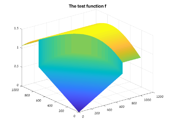
Figure 1. An example of a 2D non-smooth function

Next, in Figure 2, we present the $N\times N$ cell-average data derived from the above test function computed for $N=40$, $h=0.025$.

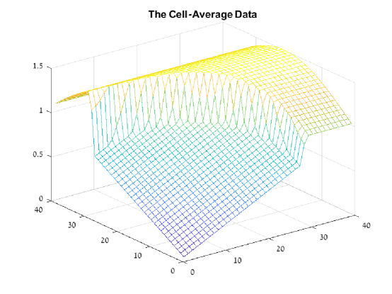
Figure 2. Cell-average data of a 2D non-smooth function

In Figure 3 we display the signature of the cell-average data. Large values are obtained at cells near the singularity curve.

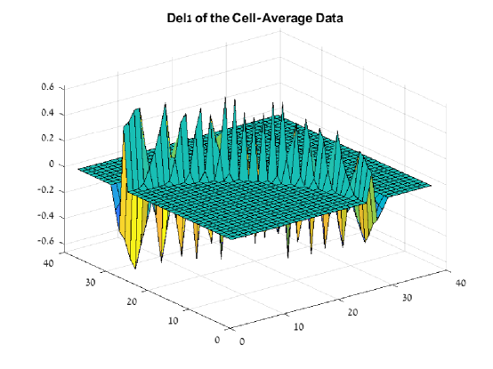
Figure 3. The signature of the Cell-average data of a 2D non-smooth function

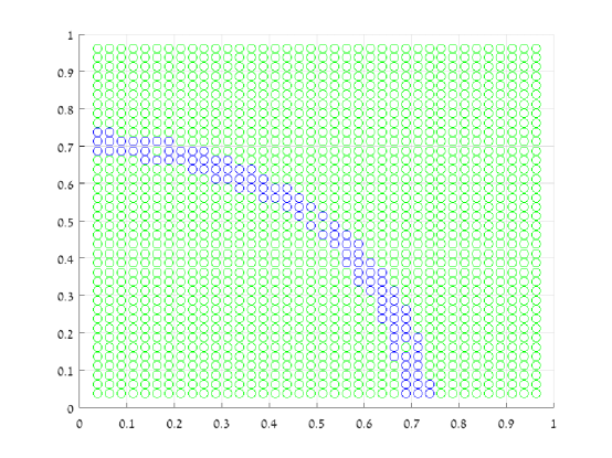
Figure 4. Cells with large signature values, in blue

We denote the cells with large signature values, i.e. $\geq 0.1max(|\sigma({\bf\bar{f}})|)$ by $U_{0}$. These cells, depicted in blue in Figure 4, serve us for sorting the rest of the cells, the green cells, into two sets $U_{1}$ and $U_{2}$ in either side of the singularity curve $\Gamma$. The sets $U_{0}$, $U_{1}$, and $U_{2}$ are considered both as sets of cells and as sets of midpoints of cells.

Now, we would like to propose an algorithm based on theoretical shreds of evidence, allowing us to develop a full theoretical analysis of our approach.

By the definition of the signature operator, the following observations follow:

Lemma 3.1.

Let $M=max(sup_{\Omega_{1}}\{|f_{1,xx}|+|f_{1,yy}|\},sup_{\Omega_{2}}\{|f_{2,xx}|+|f_{2,yy}|\})$. Then for a cell $c_{i,j}$ centered at $p_{i,j}$, if $dist(c_{i,j},\Gamma)\geq h$

$$|s_{i,j}|\leq Mh^{2},$$

and if $h/2<dist(p_{i,j},\Gamma)\leq h$

$$|s_{i,j}|\geq\delta_{i,j}/2$$

for a small enough $h$, where $\delta_{i,j}$ is the magnitude of the jump in $f$ across $\Gamma$ at the closest point to $p_{i,j}$.

Recalling Assumption 2.1(3), we suggest the following detection algorithm:

The Detection Algorithm

We let $c_{i,j}\in U_{0}$ if

$$|s_{i,j}|\geq\delta/2.$$

Using Lemma 3.1 it follows that detection algorithm identifies cells which are near $\Gamma$ if $h<\kappa h_{c}$ where

$$h_{c}=\sqrt{\frac{\delta}{M}},$$

where $\kappa$ is small enough.

In practice, we need an estimation of $\delta$. By definition, it is smaller than the minimal jump $|f_{1}-f_{2}|$ in $f$ across $\Gamma$. The first step is to distinguish the jumps computed in smooth regions $U_{1}$ or $U_{2}$ from the jumps crossing the singularity curve. Let $h^{{}^{\prime}}_{c}$ small enough such that

$$\max_{U_{1}\bigcup U_{2}}\{||\nabla f||_{1}\}h^{{}^{\prime}}_{c}<\sqrt{h^{{}^{\prime}}_{c}}$$

or equivalently

$$\max_{U_{1}\bigcup U_{2}}\{||\nabla f||_{1}\}<\frac{1}{\sqrt{h^{{}^{\prime}}_{c}}}.$$

Then, we have $|\bar{f}_{i,j}-\bar{f}_{i^{{}^{\prime}},j^{{}^{\prime}}}|<\sqrt{h^{{}^{\prime}}_{c}}$ for all $(i,j)$ and $(i^{{}^{\prime}},j^{{}^{\prime}})$ in a neighborhood of $U_{1}$ or $U_{2}$. In particular, the jumps crossing $\Gamma$ will be greater than $\sqrt{h^{{}^{\prime}}_{c}}$. Therefore, we can propose

$$\delta^{*}=\min\{|\bar{f}_{i,j}-\bar{f}_{i^{{}^{\prime}},j^{{}^{\prime}}}|\ s.t.\ |\bar{f}_{i,j}-\bar{f}_{i^{{}^{\prime}},j^{{}^{\prime}}}|>\sqrt{h^{{}^{\prime}}_{c}}\}$$

as an approximation of $\delta$. In fact, when the differences cross $\Gamma$ its absolute value is $O(1)$ (bigger than $\frac{\delta}{2}>\sqrt{h^{{}^{\prime}}_{c}}$).

Then, we can take $h\leq\kappa\min\{h_{c},h^{{}^{\prime}}_{c}\}$ where

$$\max_{U_{1}\bigcup U_{2}}\{||\nabla f||_{1}\}<\frac{1}{\sqrt{h^{{}^{\prime}}_{c}}}$$

and

$$h_{c}=\sqrt{\frac{\delta^{*}}{M}}.$$

3.2.1. A global implicit approximation of $\Gamma$

Similar to the approach in [2] we define the approximation to the singularity curve $\Gamma$ as the zero level curve of a bivariate spline function approximating a proper signed-distance function. Referring to the sets $U_{1}$, $U_{2}$ and $U_{0}$ defined above, we attach to each point $p\in U_{1}$ the value $dist(p,U_{0})+h$ and to each point $p\in U_{2}$ the value $-dist(p,U_{0})-h$. The addition of $\pm h$ is due to the observation that the ‘width’ of the set $U_{0}$ is approximately $2h$, which is the size of the support of the discrete Laplacian operator defining the signature. Now we find a smooth bivariate spline on $[0,1]^{2}$ approximating the above data on $U_{1}$ and $U_{2}$ in the least-squares sense. The zero level curve of this spline is the suggested approximation to $\Gamma$. Using a bi-cubic spline $S_{3}(x,y)$ with knots distance 0.25, we derive the approximation to $\Gamma$ presented in Figure 5, where the exact $\Gamma$ is depicted in blue and the approximation in red. We observe that the approximation is deteriorating near the two ends of the curve. A better approximation, using the same parameters, is displayed in Figure 6 for the case of a closed singularity curve $\Gamma_{2}$ defined by

$$(x-0.5)^{2}+(y-0.5)^{2}=0.1.$$ (3.6)

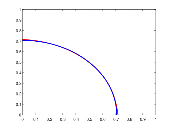
Figure 5. The singularity curve in blue and its approximation in red

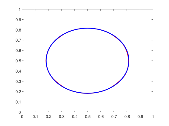
Figure 6. Approximation of a smooth closed singularity curve.

The above procedure gives a global approximation of the singularity curve with an $O(h)$ approximation order. A local piecewise linear method for approximating the singularity curve is presented in [7], and this is already an $O(h^{2})$ method. In the next section, we extend the ideas in [7] to finding an $O(h^{3})$ local approximations of the singularity curve. Further on, we use the local approximations for deriving a global $O(h^{3})$ approximation of the curve.

4. Quadratic approximation to $\Gamma$.

In this section, we introduce a quadratic approximation of the singularity curve.

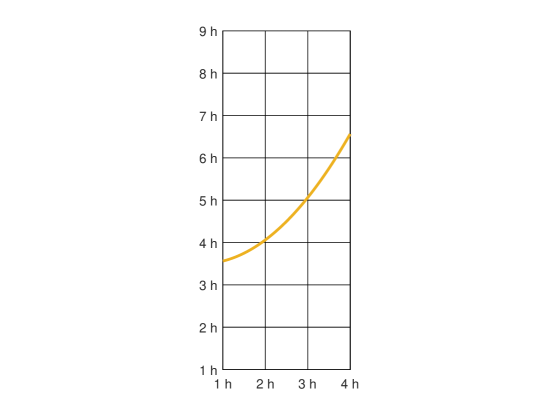
Figure 7. A zoom on a neighborhood of $\Gamma$

In [7] the authors present an algorithm that is exact for step images with a linear $\Gamma$. We suggest making an algorithm that is exact for an image that is linear on each side of $\Gamma$, and $\Gamma$ is a quadratic function. It seems that this is the minimal for obtaining an $O(h^{3})$ approximation to $\Gamma$.

Assume the function $f$ below $\Gamma$ is

$$L_{1}(x,y)=\alpha_{1}x+\beta_{1}y+\gamma_{1},$$

and the function above $\Gamma$ is

$$L_{2}(x,y)=\alpha_{2}x+\beta_{2}y+\gamma_{2}.$$

Assume also that $\Gamma$ is passing between $y=3h$ and $y=7h$ as in Figure 7 and is given by the equation

$$q(x)=ax^{2}+bx+c.$$

We are given the function cell-averages $\bar{f}_{ij}$ defined in (2.4). Using these values we would like to retrieve the parameters of the linear-quadratic model. The suggested algorithm is as follows:

• First, we find $\alpha_{1},\beta_{1},\gamma_{1}$ by matching the cell-averages of the linear model to the given cell-averages $\bar{f}_{3,2},\bar{f}_{3,3},\bar{f}_{4,3}$. This gives us a linear system for the 3 unknowns.

• Second, we find $\alpha_{2},\beta_{2},\gamma_{2}$ by matching the cell-averages of the linear model to the given cell-averages $\bar{f}_{3,9},\bar{f}_{3,8},\bar{f}_{4,8}$.

• Third, using the function parameters computed above, we look for the curve parameters $a,b,c$. This is done by matching the cell-averages of the linear model to the given cell-averages on three triplets of cells $\bar{f}_{2,4}+\bar{f}_{2,5}+\bar{f}_{2,6}+\bar{f}_{2,7}$, $\bar{f}_{3,4}+\bar{f}_{3,5}+\bar{f}_{3,6}+\bar{f}_{3,7}$, $\bar{f}_{4,4}+\bar{f}_{4,5}+\bar{f}_{4,6}+\bar{f}_{4,7}$. This matching gives a system of three quadratic equations in the unknowns $a,b,c$.

4.1. The system of quadratic equations

$$Q_{i}(a,b,c)=\bar{f}_{i,4}+\bar{f}_{i,5}+\bar{f}_{i,6}+\bar{f}_{i,7},\ \ \ \ i=2,3,4.$$ (4.1)

where

$$Q_{i}(a,b,c)\equiv h^{-2}\left(\int^{ih}_{(i-1)h}\int^{q(x)}_{3h}(L_{1}(x,y)-L_{2}(x,y))dydx+\int^{ih}_{(i-1)h}\int^{7h}_{3h}L_{2}(x,y)dydx\right).$$ (4.2)

Denoting $L_{1}(x,y)-L_{2}(x,y)=\alpha x+\beta y+\gamma$, let us expand the first integral above:

$$\int^{ih}_{(i-1)h}\int^{q(x)}_{3h}(\alpha x+\beta y+\gamma)dydx=\int^{ih}_{(i-1)h}[(\alpha x+\gamma)(q(x)-3h)+\beta/2(q(x)^{2}-(3h)^{2})]dx.$$

Approximating any other segment of $\Gamma$ can be done by transforming the coordinates so that the problem is defined in $[h,3h]\times[h,9h]$ as in Figure 7. Thus we look for $q(x)=ax^{2}+bx+c$ such that $q:[2h,3h]\ \to\ [3h,7h]$. Observing that $c=O(h)$ we may rewrite $q$ as

$$q(x)=ax^{2}+bx+ch,$$ (4.3)

where now the unknown parameters $a$, $b$ and $c$ are $O(1)$ as $h\to 0$.

Since $q(x)=ax^{2}+bx+ch$, the above integral is a quadratic form in the unknowns $a,b,c$.

4.2. Local approximation order

Let us assume that $\Gamma$ is locally defined by a $C^{3}$ function $g(x)$, and let the function $f$ be $f_{1}\in C^{2}$ below $\Gamma$ and $f_{2}\in C^{2}$ above $\Gamma$. Consider the same local neighborhood $R$ of $\Gamma$ described in Figure 7. Within $R$ there exists a local quadratic approximation $\tilde{q}(x)\sim g(x)$, $\tilde{q}(x)=\tilde{a}x^{2}+\tilde{b}x+\tilde{c}h$ such that

$$g(x)=\tilde{q}(x)+O(h^{3}).$$ (4.4)

Denoting the linear functions defined above as $\tilde{L}_{1}(x,y)\sim f_{1}(x,y)$ and $\tilde{L}_{2}(x,y)\sim f_{2}(x,y)$, they satisfy

$$f_{1}(x,y)=\tilde{L}_{1}(x,y)+O(h^{2}),$$

$$f_{2}(x,y)=\tilde{L}_{2}(x,y)+O(h^{2}),$$

in $R$, as $h\to 0$. Denoting by $\tilde{\Gamma}$ the graph of $\tilde{q}$ in $R$, by $\tilde{L}(x,y)$ the function which is $\tilde{L}_{1}$ below $\tilde{\Gamma}$ and $\tilde{L}_{2}$ above $\tilde{\Gamma}$, let us compare the cell-averages $\bar{f}_{i,j}$ of $f$ and $\bar{L}_{i,j}$ of $\tilde{L}$ within $R$. Since the area between $\Gamma$ and $\tilde{\Gamma}$ on a cell of size $h\times h$ is $O(h^{4})$, it follows that

$$\bar{f}_{i,j}=\bar{L}_{i,j}+O(h^{2}).$$ (4.5)

Let us consider the system of equations for the quadratic model for $\Gamma$. We know the system is solvable if we replace all the values $\{\bar{f}_{i,j}\}$ used for cell-average matching by the corresponding values $\{\bar{L}_{i,j}\}$. By (4.5), it follows that the system (4.1) is an $O(h^{2})$ perturbation of the solvable system

$$Q_{i}(\tilde{a},\tilde{b},\tilde{c})=\bar{L}_{i,4}+\bar{L}_{i,5}+\bar{L}_{i,6}+\bar{L}_{i,7},\ \ \ \ i=2,3,4.$$ (4.6)

Using this observation we would like to show that the solution of the system (4.1) is an $O(h^{2})$ perturbation of the solution of (4.6). Let us denote the mapping $Q:\mathbb{R}^{3}\to\mathbb{R}^{3}$, $Q(a,b,c)=(Q_{1}(a,b,c),Q_{2}(a,b,c),Q_{3}(a,b,c))^{t}$, the right hand side of the system (4.1) as $\bar{F}\in\mathbb{R}^{3}$, and the right hand side of the system (4.6) as $\bar{L}\in\mathbb{R}^{3}$. To solve the system

$$Q(a,b,c)-\bar{F}=0,$$ (4.7)

we use Newton’s iterations. Since $\bar{F}$ is a constant vector, the iterations are

$$(a^{[n+1]},b^{[n+1]},c^{[n+1]})^{t}=(a^{[n]},b^{[n]},c^{[n]})^{t}-J_{Q}(a^{[n]},b^{[n]},c^{[n]})^{-1}(Q(a^{[n]},b^{[n]},c^{[n]})-\bar{F}),$$ (4.8)

$n\geq 0$, where $J_{Q}$ is the Jacobian of $Q$.

Lemma 4.1.

Under condition 2.1(3), for a small enough $h$, $\|J_{Q}^{-1}\|_{\infty}\geq C_{J}>0$.

Proof.

It is enouth to show that $|det(J_{Q})|\geq\beta>0$ for $\beta>0$, where $\beta$ is independent upon the approximation location. For the case of constant functions $L_{1}=c_{1}$, $L_{2}=c_{2}$, it follows, by direct calculations, that

$$det(J_{Q})=2(c_{2}-c_{1})^{3}.$$

For the case of linear functions $L_{1}$, $L_{2}$, in view of condition 2.1(3), it follows by a perturbation argument that

$$|det(J_{Q})|\geq 2\delta^{3}+O(h),$$

as $h\to 0$. ∎

Proposition 4.2.

Let $\tilde{v}^{[0]}=(\tilde{a},\tilde{b},\tilde{c})^{t}$ and let $v^{[k]}=(a^{[k]},b^{[k]},c^{[k]})^{t}$ be the vectors defined by Newton’s iteration (4.8). Assuming the Hessian of $Q$ satisfies $\|H_{Q}\|_{\infty}\leq C_{H}$, and $\|\bar{L}-\bar{F}\|_{\infty}\leq Ch^{2}$, then, for a small enough $h$, Newton’s iterations converge to a solution $v^{[\infty]}$ of (4.7), and

$$v^{[\infty]}=\tilde{v}^{[0]}+O(h^{2}),$$ (4.9)

as $h$ tends to $0$.

Proof.

First we prove that for a small enough $h$

$$\|Q(v^{[k]})-\bar{F}\|_{\infty}\leq C^{2^{k}}C_{J}^{2^{k+1}-2}C_{H}^{2^{k}-1}h^{2^{k+1}},k\geq 1.$$ (4.10)

The proof is by induction. Starting with $\tilde{v}^{[0]}$, as $Q(\tilde{v}^{[0]})=\bar{L}$, by hypothesis

$$\|Q(\tilde{v}^{[0]})-\bar{F}\|_{\infty}=\|\bar{L}-\bar{F}\|_{\infty}\leq Ch^{2},$$ (4.11)

and by (4.8):

$$v^{[1]}=\tilde{v}^{[0]}-J_{Q}(\tilde{v}^{[0]})^{-1}(Q(\tilde{v}^{[0]})-\bar{F}).$$

Using Lemma 4.1, it follows that $J_{Q}(\tilde{a},\tilde{b},\tilde{c})^{-1}$ exists and is smooth and bounded in a neighborhood of $(\tilde{a},\tilde{b},\tilde{c})$, with a bound which is independent upon $h$. Then by (4.11) it follows that

$$\|v^{[1]}-\tilde{v}^{[0]}\|_{\infty}\leq CC_{J}h^{2}$$

for a small enough $h$.

Assuming (4.10) holds for $k=n$, from Newton’s iteration formula (4.8) it follows that

$$\begin{split}\|v^{[n+1]}-v^{[n]}\|_{\infty}&\leq\|J_{Q}(v^{[n]})^{-1}(Q(v^{[n]})-\bar{F})\|_{\infty}\\ &\leq C^{2^{n}}C_{J}^{2^{n+1}-1}C_{H}^{2^{n}-1}h^{2^{n+1}},\end{split}$$

for $h<0.5(CC_{J}^{2}C_{H})^{-1}$ we obtain

$$\|v^{[n+1]}-v^{[n]}\|_{\infty}\leq C_{J}^{-1}C_{H}^{-1}2^{-2^{n}}h^{2}.$$ (4.12)

The fast decay implies

$$\|v^{[n+1]}-\tilde{v}^{[0]}\|_{\infty}\leq\tilde{C}\sum_{k=1}^{n}2^{-2^{k}}h^{2},$$ (4.13)

i.e. $v^{[n+1]}$ is in a neighborhood of $\tilde{v}^{[0]}$. If we expand $Q(v^{[n+1]})$ in Taylor series about $v^{[n]}$:

$$\begin{split}Q(v^{[n+1]})=&Q\big{(}v^{[n]}-J_{Q}(v^{[n]})^{-1}(Q(v^{[n]})-\bar{F})\big{)}\\ =&Q(v^{[n]})-J_{Q}(v^{[n]})J_{Q}(v^{[n]})^{-1}(Q(v^{[n]})-\bar{F})\\ &+(J_{Q}(v^{[n]})^{-1}(Q(v^{[n]})-\bar{F}))^{t}H_{Q}(J_{Q}(v^{[n]})^{-1}(Q(v^{[n]})-\bar{F}))\\ =&\bar{F}+(J_{Q}(v^{[n]})^{-1}(Q(v^{[n]})-\bar{F}))^{t}H_{Q}(J_{Q}(v^{[n]})^{-1}(Q(v^{[n]})-\bar{F})).\end{split}$$ (4.14)

Using the induction hypothesis, it follows that

$$\begin{split}\|Q(v^{[n+1]})-\bar{F}\|_{\infty}&\leq C_{J}^{2}C_{H}(C^{2^{n}}C_{J}^{2^{n+1}-2}C_{H}^{2^{n}-1}h^{2^{n+1}})^{2}\\ &=C^{2^{n+1}}C_{J}^{2^{n+2}-2}C_{H}^{2^{n+1}-1}h^{2^{n+2}}.\end{split}$$ (4.15)

Finally, the fast decay observed in (4.12) also implies that the sequence $\{v^{[n]}\}$ is a Cauchy sequence, and therefore converging. By (4.15), it also follows that $v^{[\infty]}=\lim_{n\to\infty}v^{[n]}$ solves the quadratic system, and the result (4.9) follows from (4.13). ∎

From Proposition 4.2, it follows that the solution of the quadratic system for the unknown coefficients $a$, $b$ and $c$ of $q$ is an $O(h^{2})$ perturbation of the corresponding coefficients of $\tilde{q}$. Therefore, in view of (4.3), in the interval $[2h,3h]$,

$$q(x)=\tilde{q}(x)+O(h^{3}),$$ (4.16)

and by (4.4)

$$q(x)=g(x)+O(h^{3}).$$ (4.17)

4.3. Enhanced global curve approximation

Using the above procedure for local $O(h^{3})$ approximations to $\Gamma$, we can now improve upon the global $O(h)$ approximation presented above in Section 3.2.1, as follows:

1. Denote the union of all the locally computed quadratic approximation curves to the different sections of $\Gamma$ by $G$.

2. Overlay on $[0,1]^{2}$ a mesh of $n\times n$ points $Q$.

3. Divide $Q$ into two sets of points, $Q_{1}$ and $Q_{2}$, separated by the points in $G$.

4. Attach to each point $p\in Q_{1}$ the value $dist(p,G)$ and to each point $p\in Q_{2}$ the value $-dist(p,G)$.

5. Find a bicubic spline $S_{3}$ on $[0,1]^{2}$ approximating the above data on $Q_{1}$ and $Q_{2}$ using a local quasi-interpolation operator.

6. The zero level curve of this spline, $\tilde{\Gamma}$, is the suggested enhanced approximation to $\Gamma$.

   As we show below, $\tilde{\Gamma}$ is essentially an $O(h^{3})$ approximation of $\Gamma$.

4.3.1. Curve approximation analysis

A similar approximation quality $\tilde{\Gamma}\sim\Gamma$ is obtained if we define the spline $S_{3}$ by quasi-interpolation to the signed-distance values defined on $Q$. In the following proposition, we analyze the quality of the approximation $\tilde{\Gamma}\sim\Gamma$, obtained by quasi-interpolation, for a class of smooth singularity curves. Below we cite the basic approximation order result from [1].

Proposition 4.3.

Assume $\Gamma$ is a $C^{4}$ smooth curve in $[0,1]^{2}$ with minimal curvature radius $>R$, and such that its $R$-neighborhood is not self-intersecting and not intersecting the boundaries of $[0,1]^{2}$ . Let $Q$ be a mesh of $n\times n$ points in $[0,1]^{2}$, of mesh size $d<R/10$. Let $\Gamma$ subdivide $[0,1]^{2}$ into two domains $\Omega_{1}$ and $\Omega_{2}$, and separate the mesh points $Q$ into $Q_{1}$ and $Q_{2}$ respectively. Let us attach signed-distance values to the mesh points $Q$ as follows:

$$D(p)=dist(p,\Gamma),\ \ \ p\in Q_{1},$$

$$D(p)=-dist(p,\Gamma),\ \ \ p\in Q_{2}.$$

Let $A$ be the quasi-interpolation operator from sets of values on $Q$ to the space of bi-cubic splines on $[0,1]^{2}$ with uniform mesh of mesh size $d$, and assume $\|A\|_{\infty}<\beta$. Let $S_{\epsilon}$ be the bi-cubic spline defined by applying $A$ to the perturbed signed-distance data

$$\tilde{D}(p)=D(p)+\epsilon_{p},\ \ \ |\epsilon_{p}|\leq\epsilon,$$

and let $\Gamma_{\epsilon}$ be the zero-level curve of $S_{\epsilon}$. Then

$$dist(\Gamma,\Gamma_{\epsilon})\leq C_{0}d^{4}+\beta\epsilon.$$ (4.18)

Corollary 4.4.

Let the singularity curve $\Gamma$ satisfy the assumptions in Proposition 4.3. Let the approximate signed-distance values be defined as in Section 4.3 with $n=O(h^{-\frac{3}{4}})$, with $S_{3}$ defined using a cubic quasi-interpolation approximation operator, and the resulting approximated curve denoted by $\tilde{\Gamma}$. Then, as $h\to 0$,

$$dist(\Gamma,\tilde{\Gamma})=O(h^{3}).$$ (4.19)

Proof.

By the construction in Section 4.3, and using (4.17), it follows that the perturbation parameter in Proposition 4.3 satisfies

$$\epsilon=O(h^{3}).$$

Choosing $n=O(h^{-\frac{3}{4}})$ it follows that $d=O(h^{\frac{3}{4}})$, and the result follows by (4.18).

∎

5. Reconstructing $f$

Now that we have a third-order approximation to the singularity curve we are ready to construct the approximation to $f$. We have tested two approximation strategies.

5.1. Approximation by fitting cell-averages

One obvious strategy is by fitting the cell-averages of the approximant to the given cell-average data, at all cells. The first step is to use the local high third-order approximation for generating a high order global approximation of $\Gamma$. We suggest doing it as described in Section 3.2.1 above, i.e., finding a bi-cubic spline $S_{3}(x,y)$ approximating the signed-distance from $\Gamma$. Here the signed-distance data is computed using the piecewise quadratic approximations to $\Gamma$ discussed in the previous section. Another important rule of the resulting (implicit) approximation of the singularity curve is that it provides a simple characterization of the corresponding approximation of the two subdomains $\Omega_{1}$ and $\Omega_{2}$:

$$\begin{split}\tilde{\Omega}_{1}=\{(x,y)|S_{3}(x,y)>0\}\cap[0,1]^{2},\\ \qquad\tilde{\Omega}_{2}=\{(x,y)|S_{3}(x,y)<0\}\cap[0,1]^{2}.\end{split}$$ (5.1)

We consider approximating $f_{1}$ on $\tilde{\Omega}_{1}$ and we consider approximating $f_{2}$ on $\tilde{\Omega}_{2}$ by a linear combination of basis functions,

$$\{p_{i}\}_{i=1}^{M_{1}+M_{2}}=\{p_{i}^{[1]}\}_{i=1}^{M_{1}}\cup\{p_{i}^{[2]}\}_{i=1}^{M_{2}},$$

$$\begin{split}f_{1}(x,y)\sim\sum_{i=1}^{M_{1}}a^{[1]}_{i}p^{[1]}_{i}(x,y)\equiv P^{[1]}(x,y),\\ \qquad f_{2}(x,y)\sim\sum_{i=1}^{M_{2}}a^{[2]}_{i}p^{[2]}_{i}(x,y)\equiv P^{[2]}(x,y).\end{split}$$ (5.2)

For example, we may use two sets of bi-cubic spline basis functions, one with B-splines restricted to $\tilde{\Omega}_{1}$ and the other with B-splines restricted to $\tilde{\Omega}_{2}$.

It is convenient and worthwhile to consider the approximant in the form

$$\tilde{f}(x,y)\equiv P^{[1]}(x,y){\bf 1}_{\tilde{\Omega}_{1}}(x,y)+P^{[2]}(x,y){\bf 1}_{\tilde{\Omega}_{2}}(x,y).$$

Let us denote by ${\bf{\bar{p}}}_{i}^{[j]}$ the vector of cell-averages of $p_{i}^{[j]}$, $j=1,2$. A good approximation to $f$ implies a good approximation to the vector of cell-averages $\bf{\bar{f}}$ of $f$:

$${\bf{\bar{f}}}\sim\sum_{i=1}^{M_{1}}a_{i}^{[1]}{\bf{\bar{p}}}_{i}^{[1]}+\sum_{i=1}^{M_{2}}a_{i}^{[2]}{\bf{\bar{p}}}_{i}^{[2]}\equiv\bf{\bar{P}},$$ (5.3)

and vice versa, a good fitting of the cell averages induces a good approximation of the function. Therefore, we define the approximation to the function by solving the system of equations

$$\sum_{i=1}^{M_{1}}a_{i}^{[1]}{\bf{\bar{p}}}_{i}^{[1]}+\sum_{i=1}^{M_{2}}a_{i}^{[2]}{\bf{\bar{p}}}_{i}^{[2]}=\bf{\bar{f}},$$ (5.4)

for the coefficients $\{a_{i}^{[1]}\}_{i=1}^{M_{1}}$, $\{a_{i}^{[2]}\}_{i=1}^{M_{2}}$.

We are given $N^{2}$ cell-average data values, while the number of unknowns is $M_{1}+M_{2}$ may be different, usually smaller, than $N^{2}$. We suggest solving the system in the least-squares sense, and the challenge is to analyze the quality of the resulting approximation. We notice that an $O(h^{3})$ deviation in the position of $\Gamma$ implies an $O(h^{2})$ deviation in the computation of the cell-averages in cells containing the singularity curve. Hence, we cannot expect more than an $O(h^{2})$ approximation to $f$ using the above strategy.

5.2. Approximation of $f$ using quasi-interpolation

Two ways for directly approximating a function from cell-average values are presented in [4]. The first one is based on Taylor expansions and its advantage approach is the simplicity of both its application and its analysis. The second method is founded on quasi-interpolation theory characterized by its flexibility. In this subsection, we briefly review this technique adapting it from the general form to two dimensions (see more details in [4]).

Let start denoting by $p\in\mathbb{N}$ and for all $(x,y)\in\mathbb{R}^{2}$:

$$B_{p}\left(x,y\right)=B_{p}(x)B_{p}(y)$$

where $B_{p}$ is the $p$-degree B-spline supported on $I_{p}=\left[-\frac{p+1}{2},\frac{p+1}{2}\right]$, with equidistant knots $S_{p}=\left\{-\frac{p+1}{2},\ldots,\frac{p+1}{2}\right\}$. Given the values $\bar{f}_{i,j}$ in (2.4) and $\mathbf{n}\in\mathbb{N}^{2},$ we denote as

$$\bar{f}_{\mathbf{n},p}=\left\{\bar{f}_{n_{1}+j_{1},n_{2}+j_{2}}:0\leq|j_{l}|\leq\left\lfloor\frac{p}{2}\right\rfloor,l=1,2\right\}.$$

where $\lfloor\cdot\rfloor$ is the floor function and consider the linear operator

$$L_{p}(\bar{f}_{\mathbf{n},p})=\sum_{j_{1},j_{2}=-\left\lfloor\frac{p}{2}\right\rfloor}^{\left\lfloor\frac{p}{2}\right\rfloor}c_{p,j_{1}}c_{p,j_{2}}\bar{f}_{n_{1}+j_{1},n_{2}+j_{2}},$$ (5.5)

where the coefficients $c_{p,j}$, $j=-\left\lfloor\frac{p}{2}\right\rfloor,\ldots,\left\lfloor\frac{p}{2}\right\rfloor$ are:

$$c_{p,j}=\sum_{l=0}^{\left\lfloor\frac{p+1}{2}\right\rfloor-1}\frac{t(2l+p+1,p+1)}{{{2l+p+1}\choose{p+1}}}\sum_{i=0}^{2l}\frac{(-1)^{i}}{i!(2l-i)!}\delta_{l-i+\left\lceil\frac{p+1}{2}\right\rceil,j+1+\left\lfloor\frac{p}{2}\right\rfloor},$$ (5.6)

$\delta_{i,j}$ the Kronecker delta and $t(i,j)$ are the central factorial numbers of the first kind (see [14] and [8]) which can be computed recursively as:

$$t(i,j)=\left\{\begin{array}[]{ll}0,&\hbox{if}\,\,j>i,\\ 1,&\hbox{if}\,\,j=i,\\ t(i-2,j-2)-\left(\frac{i-2}{2}\right)^{2}t(i-2,j),&\hbox{if}\,\,2\leq j<i,\end{array}\right.$$

with

$$t(i,0)=0,\quad t(i,1)=\prod_{l=1}^{i-1}\left(\frac{i}{2}-l\right),\,\,i\geq 2,$$

and $t(0,0)=t(1,1)=1,t(0,1)=t(1,0)=0$. We show some values of $c_{p,j}$ in Table 1.

	$c_{1,j}$	$c_{2,j}$	$c_{3,j}$	$c_{4,j}$	$c_{5,j}$
$j=0$	$1$	$5/4$	$4/3$	$319/192$	$73/40$
$j=1$		$-1/8$	$-1/6$	$-107/288$	$-7/15$
$j=2$				$47/1152$	$13/240$

Table 1. $c_{p,j}$ values for $p=1,\ldots,5$. They are symmetric, $c_{p,j}=c_{p,-j}$, $j=0,\ldots,\left\lfloor\frac{p}{2}\right\rfloor$.

With these ingredients, in [4], it is proved that if $f$ is $C^{p+1}$ smooth, the operator

$$\mathcal{Q}_{p}(\bar{f})(x,y)=\sum_{\mathbf{n}\in\mathbb{Z}^{2}}L_{p+1}(\bar{f}_{\mathbf{n},p+1})B_{p}\left(\frac{x}{h}-n_{1},\frac{y}{h}-n_{2}\right)$$ (5.7)

approximates $f$ with order of accuracy $O(h^{p+1})$.

$$|f(x,y)-\mathcal{Q}_{p}(\bar{f})(x,y)|\leq Ch^{p+1}.$$ (5.8)

In the present context, we are going to use the above approximation operator with $p=3$, aiming at a global $O(h^{4})$ approximation. Hence, we shall provide two bicubic spline approximations, one on $\tilde{\Omega}_{1}$ and the other on $\tilde{\Omega}_{2}$. Considering the operator $\mathcal{Q}_{3}$, in view of the definition of $L_{3}$ and of the support of the cubic B-spline, it follows that the computation of $\mathcal{Q}_{3}(\bar{f})(x,y)$ at a given point $(x,y)$ requires the values of the cell-average values at $7\times 7$ cells surrounding that point. This presents a problem if the point $(x,y)$ is near the boundary of the domain, or near the singularity curve $\Gamma$. Such a situation is displayed in Figure 8, where the approximation at the point marked by ${\bf x}$ requires cell-average data at all the $7\times 7$ cells within the square black frame. Some of these cells are on the other side of the singularity curve. Below we suggest a constructive approach for solving this problem, assuming the following restrictions hold:

W.L.O.G., let us consider a point $(x,y)\in\tilde{\Omega}_{1}$, and assume that one of the cell-average values required for computing $\mathcal{Q}_{3}(\bar{f_{1}})(x,y)$ is either missing since $(x,y)$ is near the boundary of $[0,1]^{2}$, or, it is not a cell-average of $f_{1}$ since the cell intersects $\tilde{\Omega}_{2}$. We refer to such cells as non-valid cells, distinguishing from valid cells which are included in $\tilde{\Omega}_{1}$.

We shall re-define the value of a non-valid cell by a simple extrapolation of valid cell-average values $\bar{f}_{1}$, as follows: Considering such a non-valid cell, we look for the valid cell which is horizontally or vertically the closest to it. In Figure 8 we assume $\tilde{\Omega}_{1}$ is to the left of the curve, and the two cells marked by black dots are thus non-valid. Corresponding to the chosen direction, we interpolate four consecutive values of valid cell-averages (marked by red dots) by a cubic polynomial and use it for approximating the value of the cell-average at the non-valid cell. Assuming $f_{1}$ is $C^{4}$, the resulting extrapolated cell-average value approximates the exact cell average of the extension of $f_{1}$ within an $O(h^{4})$ accuracy.

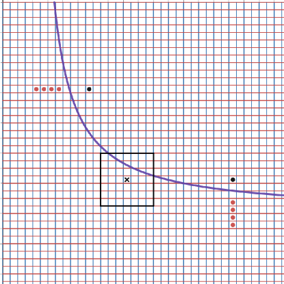
Figure 8. Function extension algorithm display

We summarize the algorithm in two steps:

• Firstly, we smoothly extend the cell-average data from $\tilde{\Omega}_{1}$ and from $\tilde{\Omega}_{2}$.

• We use the quasi-interpolation operator $\mathcal{Q}_{3}$ in each part to calculate the approximation of the functions $f_{1}$ and $f_{2}$.

The resulting approximation is defined as:

$$\tilde{f}(x,y)\equiv\mathcal{Q}_{3}(\bar{f}_{1})(x,y){\bf 1}_{\tilde{\Omega}_{1}}(x,y)+\mathcal{Q}_{3}(\bar{f}_{2})(x,y){\bf 1}_{\tilde{\Omega}_{2}}(x,y).$$ (5.9)

We note that the approximation rate $O(h^{p+1})$ of $\mathcal{Q}_{p}$ in (5.8) remains unchanged if the values of the cell-averages used for calculating $L_{p+1}$ contains $O(h^{p+1})$ errors. Therefore, considering $f_{1}$ and $f_{2}$ to be the extensions assumed in Assumption 2.1, it follows that:

$$|\big{(}f_{1}(x,y)-\mathcal{Q}_{3}(\bar{f}_{1})(x,y)\big{)}{\bf 1}_{\tilde{\Omega}_{1}}(x,y)|\leq Ch^{4},$$ (5.10)

$$|\big{(}f_{2}(x,y)-\mathcal{Q}_{3}(\bar{f}_{2})(x,y)\big{)}{\bf 1}_{\tilde{\Omega}_{2}}(x,y)|\leq Ch^{4}.$$ (5.11)

In the same way, we can construct an approximation of the function $f_{1}$ or $f_{2}$ for any order of accuracy $p+1$ using the operator $\mathcal{Q}_{p}$, Equation (5.7), always taking into account the Assumption 2.1.

In view of the above approximation results, together with Corollary 4.4, we conclude the following compact result:

Corollary 5.1.

Let $G(f)$ be the graph of $f$ and let $G(\tilde{f})$ be the graph of the approximation in (5.9), then

$$d_{H}(G(f),G(\tilde{f}))=O(h^{3}),$$ (5.12)

as $h\to 0$, where $d_{H}$ is the Hausdorff distance.

6. Conclusions

In this paper, we have presented a global and explicit reconstruction of a piecewise smooth function in two dimensions from cell-averages data. The main contributions, apart from the improvement in the approximation order, are the global and explicit nature of the resulting approximation.

The reconstruction is adapted to the presence of a smooth jump singularity curve $\Gamma$. We have proposed a global order three approximation of $\Gamma$. The principal ingredients are a signature-based detection with third-order local approximations which are exact for piecewise linear functions with quadratic edges. The local approximations are then used to define an implicit global third-order approximation of $\Gamma$. Furthermore, new approximation operators are used for defining global explicit spline approximations to the smooth parts of the function directly from the cell-average data.

Our curve approximation results apply for smooth singularity curves and non-vanishing jumps in the function. The more general case, of curves with corners and possible zero jumps at some points along a singularity curve, is a challenging future project.

References

- [1] Amat, Sergio, David Levin, Juan Ruiz.”Corrected subdivision approximation of piecewise smooth functions” ArXiv
- [2] Amat, Sergio, David Levin, and Juan Ruiz. ”A two-stage approximation strategy for piecewise smooth functions in two and three dimensions.” IMA Journal of Numerical Analysis (2021).
- [3] Amat, Sergio, Juan Ruiz, and Juan C. Trillo. ”On an algorithm to adapt spline approximations to the presence of discontinuities.” Numerical Algorithms 80.3 (2019): 903-936.
- [4] Amat, Segio, Levin, David, Ruiz, Juan and Yáñez, Dionisio F.. ”Explicit multivariate approximations from cell-average data”, submitted.
- [5] Amir, Anat, and David Levin. ”High order approximation to non-smooth multivariate functions.” Computer Aided Geometric Design 63 (2018): 31-65.
- [6] Aràndiga, F.; Cohen, A.; Donat, R.; Dyn, N. Interpolation and approximation of piecewise smooth functions. SIAM J. Numer. Anal. 43 (2005), no. 1, 41-57.
- [7] Aràndiga, F., Cohen, A., Donat, R., Dyn, N., Matei, B. ”Approximation of piecewise smooth functions and images by edge-adapted (ENO-EA) nonlinear multiresolution technques.” Applied and Computational Harmonic Analysis (2008), 24(2), 225-250.
- [8] Butzer, P.L., K. Schmidt, E. L. Stark and L. Vogt, ”Central factorial numbers; their main properties and some applications”, Numer. Funct. Anal. Optim. (1989), 10, 419–488.
- [9] Gottlieb, D, and Shu C.W., ”On the Gibbs phenomenon and its resolution”, SIAM Rev.,39(1977): 644-668.
- [10] Gottlieb, Sigal, Jae-Hun Jung, and Saeja Kim. ”A review of David Gottlieb’s work on the resolution of the Gibbs phenomenon.” Communications in Computational Physics 9.3 (2011): 497-519.
- [11] Harten, A., Multiresolution representation of data: general framework, SIAM J. Numer. Anal. 33, 1205-1256, 1996.
- [12] Lipman, Yaron, and David Levin. ”Approximating piecewise-smooth functions.” IMA journal of numerical analysis 30, no. 4 (2010): 1159-1183.
- [13] Moler, C. B., “Iterative refinement in floating point” Journal ACM, 14(2)(1967) :316–321.
- [14] Speleers, H. ”Hierarchical spline spaces: quasi-interpolants and local approximation estimates, Adv. Comput. Math. 43 (2017): 235-255.
- [15] Tadmor, E., ” Filters, mollifiers and the computation of the Gibbs phenomenon.”,Acta Numer., 16(2007): 305-378.