An equation of state for active matter

Abstract

We characterise the steady states of a suspension of two-dimensional active brownian particles (ABPs). We calculate the steady-state probability distribution to lowest order in Peclet number. We show that macroscopic quantities can be calculated in analogous way to equilibrium systems using this probability distribution. We then derive expressions for the macroscopic pressure and position-orientation correlation functions. We check our results by direct comparison with extensive numerical simulations. A key finding is the importance of many-body effective interactions even at very low densities.

Statistical mechanics tells us the probability that a system is in a certain state, as long as it is at equilibrium Plischke2005 . For instance, the degrees of freedom for any system in the canonical ensemble are sampled from the Gibbs-Boltzmann distribution, $\mathbb{P}_{eq}\propto e^{-U/(k_{B}T)}$ (where $U$ is the system’s energy). $\mathbb{P}_{eq}$ can then be used to determine macroscopic system properties, effectively reducing a large proportion of equilibrium statistical mechanics to a difficult exercise in integration. In contrast, the steady-state probability distribution of a non-equilibrium system in a non-equilibrium steady-state (NESS), $\mathbb{P}_{ss}$, is not known a-priori risken1996fokker . In fact, a NESS need not always exist. However, if a NESS exists and $\mathbb{P}_{ss}$ can be determined, one should in principle be able to apply similar techniques to equilibrium statistical mechanics on non-equilibrium systems in a NESS. Herein lies the motivation of this letter: calculating macroscopic properties of non-equilibrium systems in a NESS using methods analogous to those of equilibrium statistical mechanics.

A popular subset of non-equilibrium phenomena, which we restrict our attention to here, are “active” matter systems Gompper_2020 ; RevModPhys.85.1143 , which never reach an equilibrium state due to the presence of internal (bulk) energy sources. Early studies of these active systems were motivated by biological processes on a wide array of length scales (from e.g. fluctuations of membranes Prost_1996 to flocking birds PhysRevLett.75.1226 ; TonerTu95 ; TONER2005170 ), but has increasingly found application in synthetic man-made systems Howse2007a ; Bricard2013 .

The active system we study here, known as Active Brownian Particles (ABPs) PhysRevLett.108.235702 ; Bialk__2013 ; PhysRevLett.114.198301 ; PhysRevLett.117.038103 ; Bickmann_2020 , is a suspension of spherical colloids in a solvent, which have a mechanism of self-propulsion driving them out of equilibrium Golestanian2005 . ABPs are widely studied due to the relative simplicity of their equations of motion, while capturing the essentials of active matter systems.

Typically theoretical descriptions of active systems (such as ABPs) approximate the many-particle dynamics by an effective one-particle distribution function. For some macroscopic quantities, these single-particle distribution functions give qualitatively similar behaviour to explicit particle based simulations Bialk__2013 ; PhysRevLett.112.218304 . However quantitative comparison is only possible using (often many) phenomenological fitting parameters. Other macroscopic quantities (e.g. the pressure of an interacting active gas) which depend on particle correlations, are simply impossible to obtain using these approaches.

Theoretical frameworks which take account of the many-particle correlations, on the other hand, look formidably difficult. However recently, a generic approach to fluctuating dynamical systems highlighting the role of non-vanishing currents in non-equilibrium steady-states (NESS) was introduced, where the relaxation dynamics towards the NESS plays a key role PhysRevE.101.042107 . In particular, PhysRevE.101.042107 introduces the notion of “typical trajectories”, which we use here to construct an ansatz for $\mathbb{P}_{ss}$ amenable to analytical solution.

This letter has three main results. The first result is an explicit expression for the steady-state probability distribution of ABPs, $\mathbb{P}_{ss}$ in $2D$. The second result is an effective interaction potential for ABPs which is independent of particle orientation, but depends on many-body (as opposed to pair-wise) interactions. The third result uses $\mathbb{P}_{ss}$ to obtain an equation of state, an expression for the active brownian swim pressure C5SM01412C at low Peclet number. The van der Waals equation is a landmark in statistical mechanics generalising the ideal gas law to an equation of state for realistic gases, expressing the pressure as an expansion in density Plischke2005 . Here we obtain an equivalent for active matter by obtaining an equation of state that is an expansion in both density and activity (here encoded in Peclet number). We also compute another macroscopic average, which probes local correlations between inter-particle position and orientation. Comparison of our calculated swim pressure and the local correlation function to direct simulations yields good agreement between the two for a range of system densities.

We consider a collection of $N$ active brownian particles on a plane of area $A=L^{2}$ with periodic boundary conditions (BCs). The $3N$ degrees of freedom satisfy the system of stochastic differential equations for their positions on the plane, $\bm{r}_{i}$, and their directions $\bm{u}_{i}=(\cos\theta_{i},\sin\theta_{i})$, of self-propulsion

$$\gamma d\bm{r}_{i}(t) =(-\bm{\nabla}_{{\bm{r}_{i}}}U+\tilde{f_{P}}\bm{u}_{i})dt+\gamma\sqrt{2D_{t}}d\bm{W}_{\bm{r}_{i}}(t),$$ (1a)

$$d\theta_{i}(t) =\sqrt{2\tilde{D}_{r}}dW_{\theta_{i}}(t)\quad,\quad$$ (1b)

where $W_{\alpha}$ are as usual Wiener processes. To be concrete, the interaction potential $U$ is the sum of pair-wise (purely repulsive) Weeks-Chandler-Anderson (WCA) potentials $\mathcal{V}(r_{ij})$ with energy scale $\epsilon$. Length is measured in units of the interaction length $\sigma$, time in units of $\sigma^{2}/D_{t}$, and energy in units of $D_{t}\gamma$, where $D_{t}$ and $\gamma$ are the translational diffusion and drag, respectively. The remaining parameters in our system quantify the strength of the active force relative to fluctuations, $f_{P}\equiv\tilde{f}_{P}\sigma/D_{t}\gamma$, the relative magnitude of rotational diffusion, $D_{r}\equiv\tilde{D}_{r}\sigma^{2}/D_{t}$, and the density of particles in our system, $\rho\equiv N\sigma^{2}/A$. Our default parameters in this letter are $\epsilon/(D_{t}\gamma)=1$ and $D_{r}=3$ (the latter corresponding to a no-slip boundary condition between the particles and the solvent in equilibrium systems).

The eqns. (1) are equivalent to a Fokker-Planck equation for the probability density, $\mathbb{P}_{ss}(\vec{X},t)$ of degrees of freedom $\vec{X}=\left(\bm{r}_{1},\theta_{1},\bm{r}_{2},\theta_{2},\cdots,\bm{r}_{N},\theta_{N}\right)$,

$$\partial_{t}\mathbb{P}\!=\!\!\sum_{i}\!\big{(}\partial_{\bm{r}_{i}}\cdot(\mathbb{P}\partial_{\bm{r}_{i}}U)-f_{P}\bm{u}_{i}\cdot\partial_{\bm{r}_{i}}\mathbb{P}+\partial_{\bm{r}_{i}}^{2}\mathbb{P}+D_{r}\partial_{\theta_{i}}^{2}\mathbb{P}\big{)}$$ (2)

subject to periodic boundary conditions. The steady-state probability density $\mathbb{P}_{ss}(\vec{X})$ is a solution of ($\partial_{t}\mathbb{P}_{ss}=0$). We define a new function $\zeta(\vec{X})$ via $\mathbb{P}_{ss}(\vec{X})\propto e^{-U(\vec{X})-f_{P}\zeta(\vec{X})}\;,\;$ so that the equilibrium distribution is recovered when $f_{P}=0$. Inserting this into this Fokker-Planck equation maps the linear partial differential equation (PDE) for $\mathbb{P}_{ss}(\vec{X})$ to a non-linear PDE for $\zeta(\vec{X})$. This is helpful mathematically because $\zeta$ is less constrained than $\mathbb{P}$ and easier to approximate. To calculate $\zeta$, we make some assumptions about its form. Symmetry under exchange of particles, translational and rotational invariance imply

$$\zeta(\vec{X})=1/2\sum_{i,j\neq i}\bm{u}_{ij}\cdot\bm{r}_{ij}w(r_{ij})+\mbox{h.o.t.}\quad,$$ (3)

where $r_{ij}=|\bm{r}_{ij}|,\bm{r}_{ij}=\bm{r}_{j}-\bm{r}_{i}$, $\bm{u}_{ij}=\bm{u}_{j}-\bm{u}_{i}$ and $w(r)$ is a scalar function (see Figure 1A). We neglect terms that are nonlinear in orientation, assuming local alignment interactions are weak.

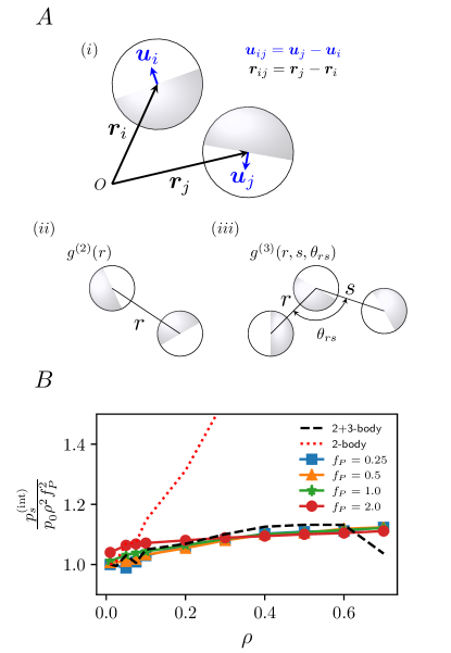
Figure 1: (A) Definitions of $\bm{u}_{ij}$ and $\bm{r}_{ij}$. Schematic of two and three body interactions. (B) Interacting swim pressure $p_{s}$ scaled by $\rho^{2}f_{P}^{2}p_{0}$, where $\rho$ is density of ABPs, $f_{P}$ is the self-propulsion force and $p_{0}^{\mathrm{th}}$ is the swim pressure at $\rho=0.01$ for the theory curve and $p_{0}^{\mathrm{sim}}={p^{\mathrm{int}}_{s}\over\rho^{2}f_{p}^{2}}(f_{P}=0.25,\rho=0.01)$ for the all experimental (simulation) data. Filled markers correspond to simulation data with self-propulsion values of $f_{P}=0.25$, $f_{P}=0.50$, $f_{P}=1.0$, and $f_{P}=2.0$, respectively. The black solid line is our theoretical prediction. The red dashed line excludes three-body correlations.

Finally, keeping terms to leading order in $f_{P}$, one arrives at the ordinary differential equation (ODE) for $w(r)$

$$w^{\prime\prime}(r)+\Omega_{1}(r)w^{\prime}(r)-\Omega_{2}(r)w(r)=\frac{\mathcal{V}^{\prime}(r)}{2r}\;,$$ (4)

where

$$\Omega_{1}(r,\xi) =3/r-\mathcal{V}^{\prime}(r)-\xi,$$ (5a)

$$\Omega_{2}(r,\xi) =D_{r}/2+\mathcal{V}^{\prime}(r)/r-\xi/r$$ (5b)

and $\xi$ fluctuates around zero, hence we set $\xi=0$ (see Methods). This ODE is solvable using standard techniques 2020SciPy-NMeth ; DORMAND198019 ; Lawrence1986SomePR . Thus, the problem of solving a $3N$ variable PDE for $\mathbb{P}_{ss}(\vec{X})$ in eqn 2 has been reduced to solving a single ODE. To solve for $w(r)$ (and hence $\zeta(\vec{X})$), we need two BC which we implement approximately as follows. First, we note that to be consistent with periodic BC’s the range of $w(r)$ (like that of $\mathcal{V}(r)$) must be less than $L/2$, i.e. $w(r)=0,r>r_{c}$ with $r_{c}<L/2$ Frenkel2002 . As we consider large systems, $L\gg 2^{1/6}$, we relax this and simply require that $w(r)\to 0$ as $r\to\infty$. Next, we note that the typical trajectories of a system in steady-state will generate (spatial) probability density currents $\bm{J}_{i}=\mathbb{P}_{ss}\bm{V}_{i}$ PhysRevE.101.042107 with

$$\bm{V}_{i}=f_{P}(\bm{u}_{i}+{\partial}_{\bm{r}_{i}}\zeta(\vec{X})),\;i\in\{1,\cdots,N\}.$$ (6)

These currents depend on $\mathbb{P}_{ss}$ and specify a family of trajectories, i.e. $\bm{V}_{i}$. This implies that we can reverse this logic and use the typical trajectories to obtain $\mathbb{P}_{ss}$ in principle. However since we need only one more BC, we only need to analyse a single trajectory. For this, we note that a trimer of three ABPs (labelled $1,2,3$) in an equilateral triangle configuration (i.e. all separated by the zero-force radius $r_{0}=2^{1/6}+O(f_{P})$) is meta-stable if their respective self-propulsion forces are directed to the centre of the trimer. This implies that the relative velocities of all three particles should be zero, i.e. $\bm{V}_{ij}=\bm{V}_{j}-\bm{V}_{i}$, then $\bm{V}_{12}=\bm{V}_{13}=\bm{V}_{23}=\bm{0}$ leading to the boundary condition

$$2^{1/6}w^{\prime}(2^{1/6})+w(2^{1/6})=-1/3.$$ (7)

.

While based on sound physical principles, the approximations we have applied are mathematically uncontrolled, and hence must be checked. We do this by empirical comparison with direct numerical simulations below.

We can now calculate macroscopic properties using steady-state distribution, $\mathbb{P}_{ss}$. The expectation value of any observable $\mathcal{O}$ is

$$\big{<}\mathcal{O}\big{>}=\frac{1}{Z}\int\bigg{(}\prod_{i=1}^{N}d^{2}r_{i}d\theta_{i}\bigg{)}\mathcal{O}(\vec{X})e^{-\frac{1}{2}\sum_{j,k\neq j}h_{jk}}$$ (8)

where $h_{ij}=\mathcal{V}(r_{ij})+f_{P}w(r_{ij})\bm{r}_{ij}\cdot\bm{u}_{ij}\;,\;$ and the normalisation constant (the “partition function”) is

$$Z=\int\bigg{(}\prod_{i=1}^{N}d^{2}r_{i}d\theta_{i}\bigg{)}e^{-\frac{1}{2}\sum_{j,k\neq j}h_{jk}}.$$ (9)

This is our first main result. Furthermore, one can explicitly integrate out orientational degrees of freedom in $\mathbb{P}_{ss}$ appendix to arrive at the marginal distribution $\mathcal{Q}_{ss}(\bm{r}_{1},\ldots,\bm{r}_{N})\sim e^{-U_{\mathrm{eff}}(\{\bm{r}_{i}\})}$ with an effective potential dependent only on particle positions ,

$$\begin{split}U_{\mathrm{eff}}=&\frac{1}{2}\sum_{i,j\neq i}\big{(}\mathcal{V}(r_{ij})-\frac{f_{P}^{2}}{2}w^{2}(r_{ij})r_{ij}^{2}\big{)}\\ &-\frac{f_{P}^{2}}{4}\sum_{\begin{subarray}{c}i,j\neq i\\ k\neq i,k\neq j\end{subarray}}w(r_{ij})w(r_{ik})\bm{r}_{ij}\cdot\bm{r}_{ik}+O(f_{P}^{3}).\end{split}$$ (10)

This effective potential constitutes the second main result of this letter. The self-propulsion $f_{P}\neq 0$ introduces a minimum in the effective interaction appendix . It also demonstrates the importance of three-body and higher-body terms, which arise due to the coupling between position and orientation degrees of freedom. We note that the three-body effective interactions have also been observed in three dimensional simulations of ABPs Turci2021 and an effective potential of the Active-Ornstein-Uhlenbeck model PhysRevLett.117.038103 . To obtain the average of a macroscopic observable where $\mathcal{O}$ is independent of orientational degrees of freedom, one may do so using $e^{-U_{\mathrm{eff}}}$ as the probability measure.

Next we use eqn. (8), to calculate the interacting swim pressure of ABPs C5SM01412C ; Solon2015 . We first remind the reader that the equation of state of a 2D fluid with temperature $T$ at equilibrium whose particles interact via a pair potential, $\mathcal{V}(r)$ is $p=k_{B}T\rho+p_{v}\;,$ with the virial interaction pressure, $\;p_{v}=-\frac{1}{4}\rho^{2}\int_{0}^{\infty}2\pi r^{2}\mathcal{V}^{\prime}(r)g^{(2)}(r)dr$ AT87 where $g^{(2)}(r)$ is the radial distribution function. We aim to obtain an equivalent for ABPs. Starting from the Kirkwood definition of the stress tensor DoiBook86 , the total pressure for ABPs may split up as $p=\rho\bigg{(}1+\frac{f_{P}^{2}}{2D_{r}}\bigg{)}+p_{v}+p_{s}^{\mathrm{int}},$ with the first term corresponding to the active ideal gas pressure (since $D_{t}\gamma_{t}=1$ in our units), the second is the virial interaction pressure $p_{v}$ appendix (present in both passive and active systems), and the last term is the interacting swim pressure $p_{s}^{\mathrm{int}}$ (which is non-zero only in the active case). The microscopic definition of $p_{s}^{\mathrm{int}}$ for the WCA potential $\mathcal{V}(r_{ij})$ is C5SM01412C

$$p_{s}^{\mathrm{int}}=-\frac{f_{p}}{4D_{r}A}\sum_{i,j\neq i}\bigg{<}\bm{u}_{ij}\cdot\bm{r}_{ij}\frac{\mathcal{V}^{\prime}(r_{ij})}{r_{ij}}\bigg{>}\;.$$ (11)

Using eqn. (8), we arrive at the expression for the steady-state swim pressure

$$p_{s}^{\mathrm{int}}=\frac{2\pi f_{P}^{2}}{4D_{r}}(\rho^{2}a_{2}(\rho)+\rho^{3}a_{3}(\rho))+O(f_{P}^{3})$$ (12)

where

$$a_{2}(\rho) \equiv\int r^{2}w(r)\mathcal{V}^{\prime}(r)g^{(2)}_{0}(r)dr,$$ (13a)

$$a_{3}(\rho) \equiv\int\int r^{2}w(r)s\mathcal{V}^{\prime}(s)G^{(3)}_{0}(r,s)drds$$ (13b)

are density dependent functions that are obtained from the passive ($f_{P}=0$) two-body: $g_{0}^{(2)}(r)$ and three-body: $G_{0}^{(3)}(r,s)$ radial distribution functions appendix   (see Figures 1A(ii) and 1A(iii)). This is our third main result.

In Figure 1B, we compare eqn. (12), (black solid line) to $p_{s}^{\mathrm{{int}}}$ directly measured from simulation. We scale the theory by its value, $p_{0}^{\mathrm{th}}$ at $\rho=0.01$ and the simulations by $p_{0}^{\mathrm{sim}}={p_{s}^{\mathrm{int}}\over\rho^{2}f_{P}^{2}}(f_{P}=0.25,\rho=0.01)$. With the scaling from eqn. (12), the simulation data does indeed collapse onto a a single curve in agreement with our calculation (the collapse is less noisy for higher densities due to more frequent collisions). We find $p_{0}^{\mathrm{sim}}/p_{0}^{\mathrm{th}}\approx 1.2$. We present simulation results for four different active force values, $f_{P}=0.25,0.50,1.0,2.0$, as a function of density. We expect the theory to begin to deviate from simulations for $f_{P}>1$. The theoretical prediction of cubic dependence in density is surprising as both $a_{2}(\rho)$ and $\rho a_{3}(\rho)$ are density dependent and so any higher dependence on $\rho$ must cancel. In fact, keeping only pair correlations gives the red dashed line which shows completely different behaviour. Clearly, three-body correlations control the dependence of $p_{s}^{\mathrm{int}}$ on density. Finally at large $\rho$ the theory curve diverges. We expect this is due to higher-body correlations which are in principle calculable in our framework.

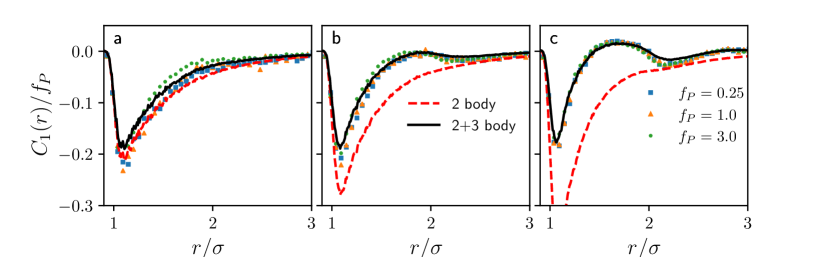
Figure 2: Pairwise orientational correlation function $C_{1}(r)$ scaled by self-propulsion $f_{P}$, vs interparticle distance $r$ for number densities (a) $\rho=0.1$, (b) $\rho=0.3$, and (c) $\rho=0.5$. Filled markers correspond to simulation data. Pink squares, green triangles, and blue stars have self-propulsion values of $f_{P}=0.25$, $f_{P}=1.0$, and $f_{P}=3.0$, respectively.

Finally, we compute the local correlation function defined as

$$C_{1}(r)\equiv\frac{1}{A}\bigg{<}\sum_{i,j\neq i}\bm{u}_{ij}\cdot\hat{\bm{r}}_{ij}\delta^{2}(\bm{r}_{ij}-\bm{r})\bigg{>}\;.$$ (14)

Physically, this quantity represents angle-averaged correlations between inter-particle orientation and inter-particle displacement, for a given spacing $r$ between pairs of particles. It is interesting to measure this function as it probes local structure of the ABPs, and so gives a more detailed picture of whether our calculation captures the mesoscale structure as well as the thermodynamic behaviour of the system. We find $C_{1}$ also depends on two-body and three-body terms,

$$\frac{C_{1}(r)}{f_{P}^{2}\rho^{2}}=-rw(r)g^{(2)}_{0}(r)-\rho\int s^{2}w(s)G^{(3)}_{0}(r,s)ds+\ldots$$ (15)

In Figure 2, we measure $C_{1}(r)$ in simulation and compare our results to those predicted by eqn. (15). Again we find that with two-body terms only that the theoretical calculation does not agree with simulations and only compares well (for all $r$) on inclusion of the three-body terms (without fitting parameters).

In conclusion, we have presented the first ab-initio calculation of the many-body steady-state probability density of states of Active Brownian Particles. This is based on a sequence of approximations that we check by numerical simulations. It is promising that despite the approximations the calculation has managed to capture the behaviour of a number of local and global observables of the system without any free parameters. This indicates that these approximations are founded on sound physical principles and capture the essential features of the non-equilibrium steady-state of ABPs at low $f_{P}$. It also suggests that they can form the starting point for a more detailed theory of these kinds of system that can be systematically improved by tightening the approximations and the assumptions behind them.

The computational resources of the University of Bristol Advanced Computing Research Centre, and the BrisSynBio HPC facility are gratefully acknowledged. TL acknowledges support of Leverhulme Trust Research Project Grant RPG-2016-147 and Bris- SynBio, a BBSRC/EPSRC Synthetic Biology Research Center (BB/L01386X/1).

References

- (1) M. Plischke and B. Bergersen, Equilibrium Statistical Physics, 3rd ed. (WORLD SCIENTIFIC, 2006), https://www.worldscientific.com/doi/pdf/10.1142/5660.
- (2) H. Risken and T. Frank, The Fokker-Planck Equation: Methods of Solution and ApplicationsSpringer Series in Synergetics (Springer Berlin Heidelberg, 1996).
- (3) G. Gompper et al., Journal of Physics: Condensed Matter 32, 193001 (2020).
- (4) M. C. Marchetti et al., Rev. Mod. Phys. 85, 1143 (2013).
- (5) J. Prost and R. Bruinsma, Europhysics Letters (EPL) 33, 321 (1996).
- (6) T. Vicsek, A. Czirók, E. Ben-Jacob, I. Cohen, and O. Shochet, Phys. Rev. Lett. 75, 1226 (1995).
- (7) J. Toner and Y. Tu, Phys. Rev. Lett. 75, 4326 (1995).
- (8) J. Toner, Y. Tu, and S. Ramaswamy, Annals of Physics 318, 170 (2005), Special Issue.
- (9) J. R. Howse et al., Physical Review Letters 99, 8 (2007), 0706.4406.
- (10) A. Bricard, J.-B. Caussin, N. Desreumaux, O. Dauchot, and D. Bartolo, Nature 503, 95 (2013).
- (11) Y. Fily and M. C. Marchetti, Phys. Rev. Lett. 108, 235702 (2012).
- (12) J. Bialké, H. Löwen, and T. Speck, EPL (Europhysics Letters) 103, 30008 (2013).
- (13) A. P. Solon et al., Phys. Rev. Lett. 114, 198301 (2015).
- (14) E. Fodor et al., Phys. Rev. Lett. 117, 038103 (2016).
- (15) J. Bickmann and R. Wittkowski, Journal of Physics: Condensed Matter 32, 214001 (2020).
- (16) R. Golestanian, T. B. Liverpool, and A. Ajdari, Physical Review Letters 94, 220801 (2005).
- (17) T. Speck, J. Bialké, A. M. Menzel, and H. Löwen, Phys. Rev. Lett. 112, 218304 (2014).
- (18) T. B. Liverpool, Phys. Rev. E 101, 042107 (2020).
- (19) R. G. Winkler, A. Wysocki, and G. Gompper, Soft Matter 11, 6680 (2015).
- (20) P. Virtanen et al., Nature Methods 17, 261 (2020).
- (21) J. Dormand and P. Prince, Journal of Computational and Applied Mathematics 6, 19 (1980).
- (22) F. S. Lawrence, Mathematics of Computation 46, 135 (1986).
- (23) D. Frenkel and B. Smit, Frenkel Smit - Understanding Molecular Simulation.pdf, 2002.
- (24) See supplementary material.
- (25) The ability to easily integrate out orientational degrees of freedom limits to being linear in . Thus, if a more generic form of were to be derived which was still linear in , one could still obtain an effective potential through this integration procedure.
- (26) F. Turci and N. B. Wilding, Physical Review Letters 126, 1 (2021), 2012.10365.
- (27) A. P. Solon et al., Nature Physics 11, 673 (2015).
- (28) M. Allen and D. Tildesley, Computer simulations of liquids (Clarendon, New York, 1987).
- (29) M. Doi and S. F. Edwards, The theory of polymer dynamics (Clarendon Press, Oxford, 1986).
- (30) is the triplet distribution function, which is related to the probability of having one particle at the origin, a second particle at radial distance , and a third particle at radial distance , with .