A model for the spread of fire blight during bloom

Abstract

We derive an infectious disease model to describe the spread of fire blight during bloom. By coupling the disease dynamics of the stationary host with the transport of the pathogen by vectors we are able to investigate the blossom blight disease cycle in a spatial setting. We use Schauder’s fixed point theorem in combination with the method of upper and lower solutions to prove the existence of travelling wave solutions when the model parameters satisfy certain constraints. By studying numerical simulations we argue that it is likely that travelling waves exist for model parameters that do not satisfy these constraints. Through a sensitivity analysis we show that ooze-carrying vectors and orchard density both play a significant role in the severity of a blossom blight epidemic when compared to the growth rate of the pathogen and the mobility of ooze-carrying vectors.

Keywords

Infectious disease    Vectored transmission   Reaction-diffusion equations   Travelling waves   Schauder fixed point theorem

1 Introduction

Fire blight, caused by the gram negative bacterium Erwinia Amylovora [1], was the first plant disease proven to be induced by bacteria. Today, over 200 years since the first printed notice of fire blight [2], this disease continues to threaten commercial apple and pear operations in Europe, North America, the Mediterranean region and the Pacific Rim [3]. When conditions are optimal, fire blight can destroy an entire orchard within a single growing season, causing significant financial losses to both the grower and to the workforce dependent on their production. In Canada, apples are the second most valuable fruit crop after berries [4]. In the province of Ontario alone, it is estimated that the Ontario apple industry contributes 351.6 million dollars to Ontario’s gross domestic product along with over 5000 full time jobs [5]. As Canadian growers shift towards planting high density orchards of fire blight susceptible cultivars [6], the threat of another severe outbreak intensifies.

The name fire blight comes from the most recognizable symptom of infection, a scorched like appearance of infected host tissue as though it had been burnt by fire. Depending on the location of infection, this disease will sometimes be referred to as, for example, twig blight, trunk blight or fruit blight. Blossom blight, the infection of an open blossom by the fire blight pathogen, is often on the mind of growers during bloom, as open blossoms provide a natural entry point for the pathogen to invade the tree [7,8], and once infection has occurred, the removal of infected tissue is the only way to prevent the subsequent death of the host. For these reasons, fire blight control strategies often focus on the prevention of blossom blight epidemics. The exact nature of how such epidemics moves through an orchard is not yet fully understood. It is the objective of this work to further our understanding of blossom blight disease dynamics so that we might infer more effective control strategies.

It is not obvious by which means E.Amylovora enters a previously blight-free orchard. It could be carried in by humans, birds, rain or insects. Once on the flower stigma, the bacteria can grow exponentially [9] and reach population sizes in the range of $10^{5}-10^{7}$ cells per flower [10, 11], as nectar provides a favourable medium for multiplication [12]. In apples, the stigmas and anthers are invaded first, which is in contrast to pears, where the invasion occurs through pistils and nectaries. In either case, free moisture from rain or dew is required for the bacteria to move from places like the stigma into natural openings of the tree [13]. When inside the flower, the pathogen can move through and multiply in the inter-cellular spaces. Large buildups of the bacterial population can then emerge from the pedicel in the form of ooze droplets. These ooze droplets can be released just days after a flower becomes infected and harbour populations of the pathogen on the scale of $10^{8}$-$10^{11}$ Colony Forming Units (CFU) per micro litre, providing a substantial amount of innoculum for secondary infections to occur [14,15]. Encased in an exopolysaccharide matrix, these bacterial populations can remain viable inside of the ooze for over a year [16].

Dissemination of E.Amylovora is primarily done by insects, wind and rain. For a comprehensive list of insects associated with the dissemination of the pathogen, see [17]. It is obvious that the large numbers of bees imported for pollination are capable of dispersing the pathogen population throughout the orchard at high speed, however, due to a lack of observed contact with secreted ooze from infected tissue, bees are not believed to play as big a role in the transmission of fire blight as previously thought. Instead, the flies, ants and other crawling insects that feed on this ooze seem to play a much bigger part in the disease cycle and require a more in-depth look. In [18], it was demonstrated that Drosophila melanogaster was capable of transporting sufficient amounts of the fire blight pathogen from ooze to healthy flowers for infection, and that the longer the insect is exposed to the secreted ooze, the more likely it is to pick it up and transport it. The effect that pollinating and non-pollinating insects have on the speed at which a blossom blight epidemic travels through an orchard, and to how severely the orchard becomes infected, is not well understood.

To understand changes in disease intensity and progress, compartmental models consisting of differential equations have been a popular approach. Many of these models take a similar form to the foundational work of Kermack and McKendrick [19], in which individual hosts are classified as either susceptible, infected or removed from the population through death or immunity. Plant disease models, including those with vectored transmission, often follow this structure as well [20,21]. What makes differential equations an attractive method of study in epidemiology is their analytical tractability. One can use the methods of calculus to formulate threshold parameters for disease outbreak or study the behaviour of the disease as time gets large. Further, systems of differential equations can lend themselves to the question of optimal control [22,23], which is of vital importance to agricultural producers in the face of disease.

Despite the economic importance of this particular plant disease, the authors found only one infectious disease model [24] to describe an outbreak of fire blight. This model was purely temporal and put an emphasis on the control of fire blight by analyzing a system of ordinary differential equations (ODEs) that allowed for the constant spraying of trees with pesticide or the removal of infected tissue. Through a sensitivity analysis, it was found that spray efficacy was the most important factor in reducing the spread of fire blight. The authors also found that a larger orchard might be more susceptible to fire blight epidemics, but since there was no spatial consideration in their model, this question remains open. In a more data-driven approach, the development of computer programs such as Maryblyt [25,26] or Cougarblight [27,28] help growers manage this disease by using weather and phenological data to output some level of infection risk. These risk prediction models are of great practical importance as they can be used to predict future states of disease pressure, allowing control strategies to be timed more efficiently. What the theoretical work in [24] and the computer programs of Maryblyt and Cougarblight do not include in their works is how spatial effects play into the propagation of fire blight infections. Since epidemics are events that take place in both time and space, an understanding of how this disease moves through an orchard seems critical.

The inclusion of spatial effects can be found in a variety of plant disease models [29, 30, 31]. Typically, a plant disease modeller assumes that an infectious agent, departing from an infectious host, is more likely to land on a neighbouring host as opposed to one further away. The study of spore dispersal often reflects this, and is summarized with detail in [32]. In the case of fire blight, the disease appears to progresses outwards from an initial foci, sometimes expanding within a row of trees faster than between them [33]. Whether this is driven primarily by rain, wind or insects, it would seem that neighbours of infected trees are in fact more likely to become infected than the trees on the other end of the orchard. This observation acts as the primary motivation for considering fire blight dynamics in a spatio-temporal setting.

Spatial consideration is also important from the viewpoint of disease management. In [34], it is shown that neglecting spatial effects can lead to sub-optimal control strategies. Current fire blight control strategies often take the form of a homogeneous application of the pesticide Streptomycin. Although an indispensable tool at the moment, getting a uniform coverage of blossoms in an orchard with high foliage can be difficult. Further, the application of such pesticides has led to an increase in antibiotic-resistant strains of the pathogen [35,36]. Integrated pest management (IPM) is an approach to pest control that aims to minimize economic, health and environmental risk [37]. Some examples of IPM strategies in the case of fire blight would be the removal of fire blight infected tissue, the bio-control of certain insects through the introduction of natural predators or the targeted delivery of control substances through pollinators [38,39,40]. In order to optimize approaches like these, it is clear that a further understanding of how vector, host and pathogen effect the disease cycle of fire blight in a spatial setting is necessary. Using a differential equation based mathematical model to explore this interplay of phenomena is the main objective of this work, and to the best of our knowledge, this is the first spatio-temporal model of fire blight and the first model to explicitly consider the pathogen population on flowers, their dissemination by bees, the secretion of ooze from infected tissue and the transportation of this ooze by non-bee vectors.

In the pages to follow, we derive a system of two semi-linear partial differential equations (PDEs) coupled to a system of three ODEs. Systems of reaction diffusion equations are common in the modelling of ecological processes [41] and in the modelling of infectious diseases [42, 43 , 44]. Sometimes, reaction-diffusion equations exhibit a fascinating phenomena; their solutions take the form of travelling waves [45,46,47]. In the context of disease models such as the one presented here, these solutions suggest that the fire blight pathogen invades the orchard at a constant speed. This makes it particularly easy to predict the future distribution of infected hosts if one already knows the current distribution and the speed at which the wave is travelling. Typically, existence of travelling wave solutions is proven for all wave speeds greater than some minimum, in which this minimum speed is expressed in terms of select model parameters. Often, it is observed that the speed of a travelling wave solution converges to this minimum speed. Then, if the model parameters that effect this minimum wave speed are controllable quantities in practice, one can essentially slow the speed at which the wave travels by altering these parameters. This makes the existence of travelling waves not just mathematically interesting, but also of practical value in both the prediction and control of the system.

The study of travelling waves, and their applications in biological and population dynamics models [48,49], has received a substantial amount of treatment [50]. However, proving their existence for nonlinear systems with more than two equations, or systems that do not generate monotone semi-flows, remains difficult. Shooting methods, like the one employed in [51], quickly become complicated when considering problems in higher dimensions. A newer approach, in which the existence of travelling wave solutions is cast as a fixed point problem, seems promising for dealing with high-dimensional and non-monotone systems. Developed primarily in the study of delay-reaction-diffusion equations [52,53], this method involves a construction of suitable upper and lower solutions, a continuous and compact mapping, and the application of Schauder’s fixed point theorem. Although this method has already been applied to a variety of models [54, 55, 56], the authors have not yet seen it’s application to a non-linear, non-monotone reaction-diffusion system in which some of the diffusion coefficients are zero.

The paper is organized as follows. In section 2, important biological assumptions are listed and from those assumptions we formulate the partially degenerate reaction-diffusion model. In section 3, we prove non-negativity, boundedness, existence and uniqueness for solutions on the bounded domain and the existence of travelling waves solutions on the unbounded domain. In section 4, we perform a series of hypothesis tests regarding the existence of travelling waves, as well as a sensitivity analysis to infer points of emphasis for blossom blight control measures. In section 5 we discuss our results and in section 6 we draw conclusions.

2 Model Formulation

The main ingredients of the model aim to capture the complex interactions between host, pathogen and vector. To do this, we couple a compartmental model for the susceptible and infected plants with two reaction-diffusion equations that describe the spatio-temporal population dynamics of the pathogen. In this work, we consider a space-time domain $\Omega$, comprised of a one dimensional row of trees having length $L$ together with non-negative time,

$$\Omega:=(x,t)\in[0,L]\times[0,\infty)\ .$$

In spite of the patchy distribution of host plants in a typical agricultural system, we consider a continuous and homogeneous density of flowers such that at each point $x\in[0,L]$, there exists a cluster of flowers of constant size $N$, all connected to the same shoot. We assume that the flowers in each cluster can be divided into three compartments. Let $S(x,t)$ denote the number of flowers at time $t$ and in the cluster at location $x$ that are susceptible to a fire blight infection. Let $I(x,t)$ denote the number of flowers in the same cluster that are infected and infectious through the production of ooze. Lastly, let $R(x,t)$ represent the number of flowers in the same cluster that are now dead and no longer infectious. A natural condition on this description is that

$$S(x,t)+I(x,t)+R(x,t)=N\ \ \text{for all }\ (x,t)\in\Omega\ .$$ (1)

In order to explicitly incorporate the effect of ooze on the disease cycle, we divide the pathogen population into two categories. Let $B(x,t)$ represent the epiphytic pathogen population at time $t$ living on the flowers in the cluster located at position $x$. Let $O(x,t)$ denote the pathogen population existing within the secreted ooze produced by an infectious blossom at time $t$ in the cluster at location $x$. Both of these compartments are measured in Colony Forming Units (CFU).

The question of boundary conditions for this system is difficult. Dirichlet conditions, for example, could be used to describe a source of the pathogen existing at the end of a row of trees, or perhaps a hostile environment in which the pathogen cannot survive. Alternatively, choosing Robin-type conditions could allow us to model both a pathogen source existing outside of the orchard as well as the in-flow and out-flow of the bacteria due to natural pollinators. Of course, we know that for a wholly susceptible orchard to become infected there must be an in-flow of the pathogen from somewhere, but since the nature of primary infection can vary drastically, this becomes a difficult process to model. Instead, we opt for homogeneous Neumann conditions. By doing this, we are essentially modelling an orchard that exists in a place of isolation, such that the in-flow and out-flow of the pathogen is minimal enough to be neglected. This is clearly not an ideal representation of an agricultural system, but it does allow for less guesswork in the modelling process and a simpler mathematical analysis. Then we have

$$\frac{\partial B}{\partial x}(0,t) =\frac{\partial B}{\partial x}(L,t)=0\ ,$$

$$\frac{\partial O}{\partial x}(0,t) =\frac{\partial O}{\partial x}(L,t)=0\ \ \ \ \text{for all time }\ t\geq 0.$$

The biological assumptions that establish the governing equations of the model are listed below.

1. The growth of epiphytic bacteria is dependent on the current size of the bacterial population and the amount of resources available for consumption. We assume the resources available for consumption are a product of the cluster’s health such that as more flowers in the cluster die, the bacterial population also dies out, but that infected and susceptible flowers provide the same amount of resources for the bacteria to survive. Also, we assume that even in a cluster of completely dead flowers, there can still exist some small population of the pathogen.

2. The production and secretion of ooze from a cluster of flowers is a function of the number of flowers currently infectious. We denote this function as $h(I(x,t))$.

3. Ooze decays at a constant rate.

4. The rate at which flowers in a cluster transition from susceptible to infectious is dependent on the local epiphytic pathogen population and the fraction of still susceptible flowers. We assume that we can model the act of invasion as a function of the local pathogen population, which we denote as $f(B(x,t))$.

5. The rate at which flowers die is a function of how infected the cluster is, such that a greater number of infected flowers weakens the cluster as a whole and drives infected flowers to death at a faster rate. We denote the function that describes this process as $g(I(x,t))$.

6. The epiphytic bacteria is transported by pollinators such as honeybees, and these pollinators move randomly throughout the orchard both within and between flower clusters. The ooze outside of the floral cup is transported primarily by flies and other non-bee pollinators that also move randomly through the orchard. In the absence of more specific foraging behaviour, these transport processes take the mathematical form of Fickian diffusion, derived as the continuous limit of a random walk process. We do not account for dissemination due to wind, rain or human.

7. The pathogen can be transferred from living within the secreted ooze to living on the surface of flower. We assume that this process is dependant on the rate at which ooze-carrying vectors visit flowers, the amount of ooze they carry, and the number of healthy flowers in the cluster. The underlying assumption here is that ooze-carrying vectors prefer to feed on the secreted ooze of infected flowers over the nectar of healthy flowers, and are more likely to deposit greater amounts of ooze to flowers (i.e pollinate for longer on the flower) when the cluster as a whole is healthy.

From the above assumptions, we derive the following set of equations,

$$B_{t}(x,t) =\underbrace{D_{1}B_{xx}(x,t)}_{\text{A6}}+\underbrace{rB(x,t)(1-\frac{B(x,t)}{K(S(x,t)+I(x,t))+\epsilon})}_{\text{A1}}+\underbrace{\mu O(x,t)S(x,t)}_{\text{A7}}$$

$$O_{t}(x,t) =\underbrace{D_{2}O_{xx}(x,t)}_{\text{A6}}+\underbrace{h(I(x,t))}_{\text{A2}}-\underbrace{\mu O(x,t)S(x,t)}_{\text{A7}}-\underbrace{\gamma O(x,t)}_{\text{A3}}$$

$$S_{t}(x,t) =\underbrace{-f(B(x,t))\cdot S(x,t)}_{\text{A4}}$$

$$I_{t}(x,t) =\underbrace{f(B(x,t))\cdot S(x,t)}_{\text{A4}}-\underbrace{g(I(x,t))\cdot I(x,t)}_{\text{A5}}$$

$$R_{t}(x,t) =\underbrace{g(I(x,t))\cdot I(x,t)}_{\text{A5}}\ .$$

The choice of functions for $h(I(x,t))$, $f(B(x,t))$ and $g(I(x,t))$ could all have interesting effects on the overall disease dynamics. For the function $h(I(x,t))$, we know that there can be no secretion of ooze if there are no flowers actively infected with the pathogen. Regardless of how one represents the production and secretion of ooze, it is biologically relevant to have $h(0)=0$. It would also seem natural to assume that this function is a monotonically increasing function of $I(x,t)$, bounded above by some constant. In this model we assume that ooze production is proportional to the number of flowers infected,

$$h(I(x,t))=\alpha I(x,t)\ .$$

This parameter $\alpha$ mediates the amount of ooze produced per infected flower per unit time, and is a biological property of the tree.

For the function that denotes invasion, $f(B(x,t))$, we know that invasion cannot occur without the presence of the pathogen. So it is biologically relevant to require $f(0)=0$. It seems natural to assume that the speed of invasion increases with the size of the local pathogen population, i.e, that $f(B(x,t))$ is an increasing function of $B(x,t)$. Here, we assume that the invasion of healthy flowers by the pathogen occurs fastest when the local epiphytic pathogen population has grown past some threshold, but that this infection rate saturates as the pathogen population grows larger than this threshold. This idea would suggest the use of a function that is sigmoidal in shape, and so we model this process using a Hill function,

$$f(B(x,t))=M_{1}\frac{(\frac{B(x,t)}{A_{1}})^{n_{1}}}{1+(\frac{B(x,t)}{A_{1}})^{n_{1}}}\ .$$ (2)

This choice of function describes an act of invasion into healthy flowers by the pathogen at a rate close to $M_{1}$ when the pathogen population is greater than $A_{1}$. When the pathogen population is below $A_{1}$, the rate of invasion remains closer to zero. The exponent $n_{1}$ can be used to change how sensitive this process is in relation to the threshold parameter $A_{1}$. When $n_{1}$ is high, the pathogen population must be very close to or greater than $A_{1}$ for invasion to occur at the rate $M_{1}$ and not zero, whereas if $n_{1}$ is small, invasion can still occur at a relatively similar rate to $M_{1}$ even when the pathogen population is lower than $A_{1}$.

An important distinction between diseases in trees and diseases in animals is that trees respond to infection by attempting to trap the infectious agent in some compartmentalized section of the tree. In light of this, we assume that when a flower becomes infected with fire blight, the tree expends part of its resources in an attempt to prevent the further invasion of the pathogen into the stems and branches, and it does this at the cost of the health of the cluster. Further, we assume that the defense mechanism of the tree activates in response to the surpassing of some threshold of infection, or in other words, it does not sacrifice the health of the cluster when only a small portion of the cluster is infected. To model this process, we are interested in a death rate function $g(I(x,t)$ that remains close to zero when the number of infected flowers is below some threshold and close to a maximum death rate when the number of infected flowers surpasses this threshold. This function should be an increasing function of $I(x,t)$ that asymptotically gets closer to the maximum death rate as $I(x,t)$ increases. In this work, we once again consider a Hill function with a switching point,

$$g(I(x,t))=M_{2}\frac{(\frac{I(x,t)}{A_{2}})^{n_{2}}}{1+(\frac{I(x,t)}{A_{2}})^{n_{2}}}\ .$$ (3)

This specific choice of function allows for infected flowers to remain alive for longer provided the total number of infected flowers in the cluster remains below the threshold $A_{2}$. Once the infected population surpasses $A_{2}$, infected flowers begin to die at a maximum rate of $M_{2}$, as the tree has begun to redirect resources that would otherwise be used to keep those flowers alive. As in the case of $f(B(x,t))$, the exponent $n_{2}$ controls the sensitivity of this process in relation to the threshold $A_{2}$.

Including these functions in the governing equations and incorporating the Neumann boundary conditions give us the full model for blossom blight spread,

$$B_{t}(x,t) =D_{1}B_{xx}(x,t)+rB(x,t)\left(1-\frac{B(x,t)}{K(S(x,t)+I(x,t))+\epsilon}\right)+\mu S(x,t)O(x,t)$$ (4)

$$O_{t}(x,t) =D_{2}O_{xx}(x,t)+\alpha I(x,t)-\mu S(x,t)O(x,t)-\gamma O(x,t)$$ (5)

$$S_{t}(x,t) =-M_{1}\frac{(\frac{B(x,t)}{A_{1}})^{n_{1}}}{1+(\frac{B(x,t)}{A_{1}})^{n_{1}}}\cdot S(x,t)$$ (6)

$$I_{t}(x,t) =M_{1}\frac{(\frac{B(x,t)}{A_{1}})^{n_{1}}}{1+(\frac{B(x,t)}{A_{1}})^{n_{1}}}\cdot S(x,t)-M_{2}\frac{(\frac{I(x,t)}{A_{2}})^{n_{2}}}{1+(\frac{I(x,t)}{A_{2}})^{n_{2}}}\cdot I(x,t)$$ (7)

$$R_{t}(x,t) =M_{2}\frac{(\frac{I(x,t)}{A_{2}})^{n_{2}}}{1+(\frac{I(x,t)}{A_{2}})^{n_{2}}}\cdot I(x,t)\ ,$$ (8)

$$\frac{\partial B}{\partial x}(0,t) =\frac{\partial B}{\partial x}(L,t)=0\ ,$$ (9)

$$\frac{\partial O}{\partial x}(0,t) =\frac{\partial O}{\partial x}(L,t)=0\ .$$ (10)

$$B(x,0)=B_{0}(x)\geq 0\ ,$$ (11)

$$O(x,0)=O_{0}(x)\geq 0\ ,$$ (12)

$$S(x,0)=S_{0}(x)\geq 0\ ,$$ (13)

$$I(x,0)=I_{0}(x)\geq 0\ ,$$ (14)

$$R(x,0)=R_{0}(x)\geq 0\ \ \ \text{for all }x\in[0,L]\ \ ,$$ (15)

$$S_{0}(x)+I_{0}(x)+R_{0}(x)=N\ \ \text{for all }x\in[0,L]\ .$$ (16)

For a time scale, we work in the units of days. Since bloom typically lasts a few weeks, and since control strategies change daily with the weather, this appears to be the most appropriate. A full list of the model parameters and their units is presented in Table 1.

Table 1: Model parameters, their description and units.

Parameter	Description	Units
$N$	Number of flowers in each cluster	Flower
$D_{1}$	Diffusion coefficient for transport by bees.	$\text{Meters}^{2}\ \cdot\text{Day}^{-1}$
$D_{2}$	Diffusion coefficient for transport by ooze-carrying vectors.	$\text{Meters}^{2}\ \cdot\text{Day}^{-1}$
$K$	Epiphytic E.Amylovora carrying capacity of each cluster.	$\text{CFU}\cdot\ \text{Flower}^{-1}$
$\epsilon$	Carrying capacity of a completely dead cluster.	CFU
$r$	Growth rate of epiphytic E.Amylovora.	$\text{Day}^{-1}$
$\mu$	Flower-visiting rate of ooze-carry vectors.	$\text{Day}^{-1}\cdot\ \text{Flower}^{-1}$
$\gamma$	Rate of decay for secreted ooze.	$\text{Day}^{-1}$
$M_{1}$	Maximum infection rate.	$\text{Day}^{-1}$
$M_{2}$	Maximum death rate.	$\text{Day}^{-1}$
$\alpha$	Rate of ooze secretion.	$\text{CFU}\cdot\text{Day}^{-1}\cdot\ \text{Flower}^{-1}$
$A_{1}$	Threshold parameter for invasion of epiphytic E.Amylovora.	CFU
$A_{2}$	Threshold parameter for the accelerated death of clusters.	Flower
$n_{1}$	Hill function parameter for invasion function.	—
$n_{2}$	Hill function parameter for death-rate function.	—

3 Mathematical Results

3.1 Existence and uniqueness for the initial boundary value problem

Before proving the existence and uniqueness of solutions, we start with the following lemma.

Lemma 3.1.

Solutions to the system (4)-(16) remain non-negative for all time $t\in[0,+\infty)$ and are bounded above by positive constants.

Proof.

First we show that the ODE system (6)-(8) remains non-negative and bounded. To see non-negativity for $S(x,t)$, we have that

$$-f(B(x,t))=-M_{1}\frac{(\frac{B(x,t)}{A_{1}})^{n_{1}}}{1+(\frac{B(x,t)}{A_{1}})^{n_{1}}}\geq-M_{1}\ .$$

Then the time derivative of $S(x,t)$ is bounded below by

$$S_{t}(x,t)\geq-M_{1}S(x,t)\ .$$

Consider then the lower solution for $S(x,t)$,

$$\underline{S}_{t}(x,t)=-M_{1}\underline{S}(x,t)\ .$$

Clearly, if the initial conditions are the same, we would have

$$S(x,t)\geq\underline{S}(x,t)\ \ \text{for all }(x,t)\in\Omega\ .$$

We can solve for $\underline{S}$, finding

$$\underline{S}(x,t)\ =\ S_{0}(x)e^{-M_{1}t}\ .$$

Since the initial conditions are non-negative, it follows that

$$S(x,t)\geq 0\ \ \text{for all }(x,t)\in\Omega\ .$$

We can prove non-negativity for $I(x,t)$ in the same way. For now, assume $B(x,t)$ remains positive. We have that

$$-g(I(x,t))\cdot I(x,t)=-M_{2}\frac{(\frac{I(x,t)}{A_{2}})^{n_{2}}}{1+(\frac{I(x,t)}{A_{2}})^{n_{2}}}\cdot I(x,t)\geq-M_{2}I(x,t)\ .$$

Then by the non-negativity of $S(x,t)$ and $B(x,t)$, one can see that

$$I_{t}(x,t)\ \geq-M_{2}I(x,t)\ .$$

By the same argument above, we can find a lower solution for $I(x,t)$ of the form

$$\underline{I}(x,t)=I_{0}(x)e^{-M_{2}t}\ ,$$

from which it follows that

$$I(x,t)\geq 0\ \ \text{for all }(x,t)\in\Omega\ .$$

Since $I(x,t)$ remains non-negative, by (8) and (15) it is clear that

$$R(x,t)\ \geq\ 0\ \ \ \ \text{for all }(x,t)\in\Omega\ .$$

To see that the ODE system (6)-(8) with initial conditions (11)-(16) remains bounded for all time, simply add (6)-(8) to see that condition (1) is preserved. By the non-negativity of the ODE compartments we must then have

$$0\leq S(x,t) \leq N,$$

$$0\leq I(x,t) \leq N,$$

$$0\leq R(x,t) \leq N\ \ \ \text{for all }(x,t)\in\Omega\ .$$

Using the non-negativity and upper bounds of the ODE system we can prove that $O(x,t)$ remains non-negative. By the non-negativity of $I(x,t)$, and the upper bound of $N$ for $S(x,t)$, one can see that

$$O_{t}(x,t)\geq D_{2}O_{xx}(x,t)-(\mu+\gamma)\cdot N\cdot O(x,t)\ .$$

Then for identical initial conditions we can construct a lower solution $\underline{O}(x,t)$ satisfying

$$\underline{O}_{t}(x,t)=D_{2}\underline{O}_{xx}(x,t)-(\mu+\gamma)\cdot N\cdot\underline{O}(x,t)\ ,$$

such that

$$O(x,t)\geq\underline{O}(x,t)\ \ \text{for all }(x,t)\in\Omega\ .$$

Consider the ordinary differential equation

$$\frac{dw}{dt}(t)=-(\mu+\gamma)\cdot N\cdot w(t)\ \ ,\ 0\leq w(0)\leq\min_{x\in[0,L]}O_{0}(x)\ \ ,$$

where $w(0)$ is homogeneously distributed through the spatial domain. Since $w(t)$ solves the equation for $\underline{O}(x,t)$, as well as the Neumann boundary conditions, by a comparison theorem (for example, Theorem 10.1 in [57]) we have that

$$\underline{O}(x,t)\geq w(t)\ \ \ \text{for all}\ \ (x,t)\in\Omega\ .$$

It is easy to find an explicit solution for $w(t)$,

$$w(t)=w(0)e^{-(\mu+\gamma)\cdot N\cdot t}\ ,$$

which is evidently non-negative for all time.

By a similar argument, to see that $O(x,t)$ remains bounded, let $I(x,t)$ achieve its upper bound of $N$ and let $S(x,t)$ achieve its lower bound of zero to see that

$$O_{t}(x,t)\leq D_{2}O_{xx}(x,t)+\alpha N-\gamma O(x,t)\ .$$

For identical initial conditions, there exists an upper solution $\overline{O}(x,t)$ that solves

$$\overline{O}_{t}(x,t)=D_{2}\overline{O}_{xx}(x,t)+\alpha N-\gamma\overline{O}(x,t)\ ,$$

such that

$$\overline{O}(x,t)\geq O(x,t)\ \ \ \text{for all}\ \ (x,t)\in\Omega\ .$$

Consider now the ordinary differential equation

$$\frac{dv}{dt}(t)=\alpha N-\gamma v(t)\ \ ,\ \ v(0)\geq\max_{x\in[0,L]}O_{0}(x)\ \ ,$$

where $v(0)$ is homogeneously distributed through the space domain. Clearly, $v(t)$ is a solution to the equation for $\overline{O}(x,t)$ together with the Neumann conditions, allowing us to conclude that

$$O(x,t)\leq v(t)\ \ \ \text{for all}\ \ (x,t)\in\Omega\ .$$

It is easy to see that

$$v(t)\longrightarrow\frac{\alpha N}{\gamma}\ \ \text{as}\ \ t\longrightarrow+\infty\ .$$

By comparison we must have

$$O(x,t)\ \leq\ \max\{\max_{x\in[0,L]}O_{0}(x),\frac{\alpha N}{\gamma}\}\ \ \ \ \text{for all}\ \ (x,t)\in\Omega\ .$$ (17)

Non-negativity of $B(x,t)$ once again comes from a lower solution argument. Consider a lower solution of $B(x,t)$ of the form

$$u_{t}(t)=ru(t)\left(1-\frac{u(t)}{\epsilon}\right),\ \ 0\leq u(0)\leq\min_{x\in[0,L]}B_{0}(x)\ \ ,$$

where $u(0)$ is homogeneously distributed through the spatial domain. One can find a solution for this through separation of variables,

$$u(t)=\frac{u(0)\epsilon e^{rt}}{\left(\epsilon-u(0)\right)+u(0)e^{rt}}\ .$$

It is easy to see that this remains positive for all time, and by comparison,

$$B(x,t)\geq 0\ \ \text{for all}\ \ (x,t)\in\Omega\ .$$

To see that $B(x,t)$ is bounded, we use the fact that $O(x,t)$ remains bounded. Define $C_{O}$ to be

$$C_{O}:=\max\left\{\ \max_{x\in[0,L]}O_{0}(x),\ \frac{\alpha N}{\gamma}\right\}.$$

Using the same arguments as above, we can analyze a spatially homogeneous super solution of the form

$$y(t)=ry(t)\left(1-\frac{y(t)}{K\cdot N+\epsilon}\right)+\mu C_{O}\ ,$$

in which we find a globally attractive fixed point $y_{e}$, where

$$y_{e}=\frac{K\cdot N+\epsilon}{2}\left(1\pm\sqrt{1+\frac{4\mu C_{O}}{r(K\cdot N+\epsilon)}}\right)\ .$$

It follows from comparison that

$$B(x,t)\ \leq\ \max\ \left\{\ \frac{K\cdot N+\epsilon}{2}\left(1+\sqrt{1+\frac{4\mu C_{O}}{r(K\cdot N+\epsilon)}}\right),\ \max_{x\in[0,L]}\{B_{0}(x)\}\ \right\}\ \ \ \text{for all}\ \ (x,t)\in\Omega\ .$$

This completes our proof of Lemma 3.1.

∎

This leads us to our proof for existence and uniqueness. Let $BC\cap L^{\infty}$ denote the intersection between the space of functions that are bounded and uniformly continuous on $\mathbb{R}$ and the space of $L^{\infty}$-integrable functions.

Theorem 3.2.

For a set of non-negative initial conditions where

$$\max_{x\in[0,L]}\{B_{0}(x)\} \leq\frac{K\cdot N+\epsilon}{2}\left(1+\sqrt{1+\frac{4\mu\frac{\alpha}{\gamma}}{r(K+\epsilon)}}\right)\ ,$$

$$\max_{x\in[0,L]}\{O_{0}(x)\} \leq\frac{\alpha N}{\gamma}\ ,$$

$$S_{0}(x),\ I_{0}(x),\ R_{0}(x) \leq N\ ,$$

the system (4)-(16) admits a unique solution on any time interval $t\in[0,T]$ such that

$$B(x,t),\ O(x,t),\ S(x,t),\ I(x,t),\ R(x,t)\in C([0,T],BC\cap L^{\infty})\ .$$

Proof.

It follows from Lemma 3.1 that the solutions of system (4)-(16) arising from the constraints on these initial conditions remain non-negative and bounded above by the constants on the right hand side of each inequality for all time. Using definition 14.1 and theorems 14.2-14.4 in Smoller’s book [57], one can use Banach’s fixed point theorem and construct a mapping in the admissible Banach space $BC\cap L^{\infty}$ such that the mapping is invariant and admits a unique fixed point in $BC\cap L^{\infty}$. This fixed point gives a unique solution for the system up to some time $t_{0}$. The time $t_{0}$ depends only on the non-linearity of the system and the a-priori upper bound on the initial conditions, and since the solutions remain bounded for all time by these constants, we can iterate this mapping by taking the values of the solution at $t_{0}$ as initial conditions to extend this solution over any time interval [0,T]. It follows then that we get a unique solution

$$B(x,t),\ O(x,t),\ S(x,t),\ I(x,t),\ R(x,t)\in C([0,T],BC\cap L^{\infty})\ \ \ \text{for all }t,\ 0\leq t\leq T\leq\infty\ .$$

∎

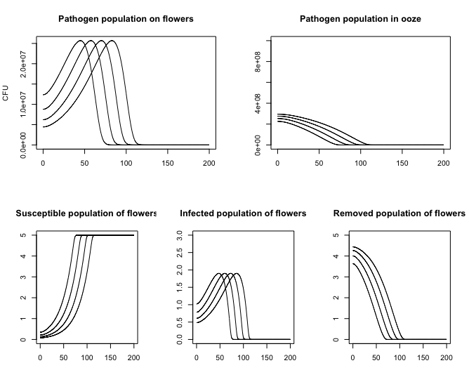
Figure 1: An illustrative simulation to show the typical behaviour of the numerical solutions. For initial conditions, we took the pathogen population existing on flowers to be zero everywhere except for $10^{6}$ CFUs existing at $x=0$. The amount of ooze, infected population and removed population are initially set to zero everywhere, while the number of susceptibles are set to five flowers in each cluster existing at each point in space. Pictured above are snapshots of the solution at 4, 4.5, 5 and 5.5 days.

3.2 Travelling Waves

In Figure 1, it appears as though the solutions of the system are travelling through the spatial domain with a constant shape and speed. Motivated by these simulations, we dedicate this section to studying the existence of travelling wave solutions for our coupled ODE-PDE system. By identifying a minimum wave speed for which solutions exist, and expressing this minimum speed in terms of model parameters, we might uncover which biological interactions drive new infections to occur throughout the orchard.

Let $f(\cdot)$ denote the Hill function in equation (2), and let $g(\cdot)$ denote the Hill function in (3). Let $K_{f}$ and $K_{g}$ be the lipschitz coefficients of $f(\cdot)$ and $g(\cdot)$ respectively. Consider the system (4)-(8) over the entire real line. If we make the transformation of variables to the moving reference frame $z=x+ct$, the system becomes

$$cB^{\prime}(z)-D_{1}B^{\prime\prime}(z) =rB(z)(1-\frac{B(z)}{K(S(z)+I(z))+\epsilon})+\mu\cdot O(z)\cdot S(z)$$ (18)

$$cO^{\prime}(z)-D_{2}O^{\prime\prime}(z) =\alpha\cdot I(z)-\mu\cdot O(z)\cdot S(z)-\gamma O(z)$$ (19)

$$cS^{\prime}(z) =-f(B(z))S(z)$$ (20)

$$cI^{\prime}(z) =f(B(z))S(z)-g(I(z))I(z)$$ (21)

Here, we have ommitted the equation for $R(z)$ as it can be characterized entirely by $S(z)$ and $I(z)$.

We call system (18)-(21) the travelling wave system, since the solutions of this system, if it admits any, would be travelling wave solutions to the original system (4)-(8). The question is; for which wave speeds $c$ does the system (18)-(21) admit travelling wave solutions such that the solutions asymptotically converge in the following ways,

$$B(-\infty) =0, O(-\infty) =0, S(-\infty) =N, I(-\infty) =0,$$

$$B(+\infty) =\epsilon, O(+\infty) =0, S(+\infty) =0, I(+\infty) =0\ ?$$

Here, $B(-\infty)=0$ means $\lim_{z\longrightarrow-\infty}B(z)=0$, etc.

To prove that this travelling wave system does indeed admit such solutions, we take a similar (if not identical) approach as in [52,53,54,55,56]: First, we construct an integral map such that a fixed point of this mapping would also be a solution to the travelling wave system. Then, we use pairs of upper and lower solutions to define a suitable Banach space for the integral map to operate on. We prove that the integral map is invariant, continuous and compact on the Banach space with respect to the appropriate norm. By Schauder’s fixed point theorem, this gives us a fixed point of the mapping in the Banach space and hence a solution to the travelling wave system. Lastly, we show that any solution found in this Banach space must satisfy a specific set of boundary conditions.

What sets the following proof apart from the usual travelling wave proofs involving this method is that our system has two PDEs coupled to two ODEs, whereas the other works have focused mostly on systems consisting entirely of PDEs. As a result, we have had to define different integral operators for the ODE components of the system. The lack of a diffusion term, along with the non-linearity of the ODE system, made finding suitable upper and lower solutions challenging, forcing us to simplify the interaction between the functions $f(\cdot)$ and $g(\cdot)$ in the differential equation for the infected population. As a result, the travelling wave proof holds only if the model parameters satisfy certain constraints, some of which are very strong and offer little biological interpretation.

Theorem 3.3.

Let all parameters be positive, $D_{2}\leq D_{1}$, $n_{1}=n_{2}+1$ and

$$M_{1} \leq g(N)\ ,$$

$$\alpha^{n_{1}}M_{1}N\left(A_{2}^{n_{2}}+N^{n_{2}}\right) \leq A_{1}^{n_{1}}M_{2}\gamma^{n_{1}}\ .$$

For all wave speeds

$$c\geq 2\sqrt{D_{1}(r+\mu N)}\ ,$$

there exists a non-negative solution to the travelling wave system (18)-(21) that satisfies

$$B(-\infty) =0, O(-\infty) =0, S(-\infty) =N, I(-\infty) =0,$$

$$B(+\infty) =\epsilon, O(+\infty) =0, S(+\infty) =0, I(+\infty) =0.$$

Proof.

To see this, take the following steps.

Step 1

Define the differential operator

$$\Delta=(\Delta_{B},\Delta_{O},\Delta_{S},\Delta_{I})\ ,$$

such that

$$\Delta_{B}(B)(z):= \ -D_{1}B^{\prime\prime}(z)+cB^{\prime}(z)+\alpha_{B}B(z)\$$

$$\Delta_{O}(O)(z):= \ -D_{2}O^{\prime\prime}(z)+cO^{\prime}(z)+\alpha_{O}O(z)\$$

$$\Delta_{S}(S)(z):= \ cS^{\prime}(z)+\alpha_{S}S(z)\$$

$$\Delta_{I}(I)(z):= \ cI^{\prime}(z)+\alpha_{I}I(z)\ .$$

The constants $\alpha_{B},\alpha_{O},\alpha_{S},\alpha_{I}$ need to be taken sufficiently large, and will be determined later.

The characteristic roots of $\Delta_{B}$ and $\Delta_{O}$ are found to be

$$\lambda_{B}^{\pm}:= \ \frac{c\pm\sqrt{c^{2}+4D_{1}\alpha_{B}}}{2D_{1}}$$

$$\lambda_{O}^{\pm}:= \ \frac{c\pm\sqrt{c^{2}+4D_{2}\alpha_{O}}}{2D_{2}}\ .$$

Define

$$\rho_{B}:= D_{1}(\lambda_{B}^{+}-\lambda_{B}^{-})=\sqrt{c^{2}+4D_{1}\alpha_{B}}$$

$$\rho_{O}:= D_{2}(\lambda_{O}^{+}-\lambda_{O}^{-})=\sqrt{c^{2}+4D_{2}\alpha_{O}}\ .$$

For any positive choices of $D_{1},D_{2},\alpha_{B}$ and $\alpha_{O}$, there exists a positive value $\mu_{0}$ such that if

$$\mu_{0}^{+} =\mu_{0}\ ,$$

$$\mu_{0}^{-} =-\mu_{0}\ ,$$

then

$$\lambda_{B}^{-}<\mu^{-}_{0}<0<\mu^{+}_{0}<\lambda_{B}^{+}\ \$$

$$\lambda_{O}^{-}<\mu^{-}_{0}<0<\mu^{+}_{0}<\lambda_{O}^{+}\ .$$

Pick any $\mu_{0}$ such that the above inequalities hold. For functions $B(z),O(z),S(z)$ and $I(z)$ in the space

$$C_{\mu^{-}_{0},\mu^{+}_{0}}(\mathbb{R}):=\{h(z)\in C(\mathbb{R})\ \ |\ \sup_{z\leq 0}|h(z)e^{-\mu^{-}_{0}z}|+\sup_{z\geq 0}|h(z)e^{-\mu^{+}_{0}z}|<\infty\}\ ,$$

the inverse operators for each component of $\Delta$ have the following integral representation

$$(\Delta_{B}B)^{-1}(z):= \frac{1}{\rho_{B}}\left(\int_{-\infty}^{z}e^{\lambda_{B}^{-}(z-y)}B(y)dy+\int_{z}^{\infty}e^{\lambda_{B}^{+}(z-y)}B(y)dy\right)$$

$$(\Delta_{O}O)^{-1}(z):= \frac{1}{\rho_{O}}\left(\int_{-\infty}^{z}e^{\lambda_{O}^{-}(z-y)}O(y)dy+\int_{z}^{\infty}e^{\lambda_{O}^{+}(z-y)}O(y)dy\right)$$

$$(\Delta_{S}S)^{-1}(z):= \frac{1}{c}\left(\int_{-\infty}^{z}e^{-\frac{\alpha_{S}}{c}(z-y)}S(y)dy+cS(-\infty)e^{-\frac{\alpha_{S}}{c}(z+\infty)}\right)$$

$$(\Delta_{I}I)^{-1}(z):= \frac{1}{c}\left(\int_{-\infty}^{z}e^{-\frac{\alpha_{I}}{c}(z-y)}I(y)dy+cI(-\infty)e^{-\frac{\alpha_{I}}{c}(z+\infty)}\right)\ .$$

To see that this is in fact the inverse operator for $\Delta_{S}(S)(z)$, we calculate

$$(\Delta_{S}^{-1})(\Delta_{S}S)(z) =\frac{1}{c}\left(\int_{-\infty}^{z}e^{-\frac{\alpha_{S}}{c}(z-y)}(cS^{\prime}(y)+\alpha_{S}S(y))dy+cS(-\infty)e^{-\frac{\alpha_{S}}{c}(z+\infty)}\right)$$

$$=\frac{1}{c}\left(\int_{-\infty}^{z}e^{-\frac{\alpha_{S}}{c}(z-y)}cS^{\prime}(y)dy+\int_{-\infty}^{z}e^{-\frac{\alpha_{S}}{c}(z-y)}\alpha_{S}S(y)dy+cS(-\infty)e^{-\frac{\alpha_{S}}{c}(z+\infty)}\right)\ ,$$

whereby applying integration by parts on the first integral yields

$$(\Delta_{S}^{-1})(\Delta_{S}S)(z)= \frac{1}{c}\bigg{(}cS(y)e^{-\frac{\alpha_{S}}{c}(z-y)}\bigg{|}_{-\infty}^{z}-\int_{-\infty}^{z}e^{-\frac{\alpha_{S}}{c}(z-y)}\alpha_{S}S(y)dy$$

$$+\int_{-\infty}^{z}e^{-\frac{\alpha_{S}}{c}(z-y)}\alpha_{S}S(y)dy+cS(-\infty)e^{-\frac{\alpha_{S}}{c}(z+\infty)}\bigg{)}$$

$$= \frac{1}{c}\left(cS(y)e^{-\frac{\alpha_{S}}{c}(z-y)}\bigg{|}_{-\infty}^{z}+cS(-\infty)e^{-\frac{\alpha_{S}}{c}(z+\infty)}\right)$$

$$= \frac{1}{c}\left(cS(z)-cS(-\infty)e^{-\frac{\alpha_{S}}{c}(z+\infty)}+cS(-\infty)e^{-\frac{\alpha_{S}}{c}(z+\infty)}\right)$$

$$= S(z)\ .$$

The calculation is identical for $\Delta_{I}^{-1}$ and similar for $\Delta_{B}^{-1}$ and $\Delta_{O}^{-1}$.

The above inverse operators can be shown to solve

$$-D_{1}(\Delta_{B}^{-1}B(z))^{\prime\prime}+c(\Delta_{B}^{-1}B(z))^{\prime}+\alpha_{B}(\Delta_{B}^{-1}B(z)) =B(z)$$ (22)

$$-D_{2}(\Delta_{O}^{-1}O(z))^{\prime\prime}+c(\Delta_{O}^{-1}B(z))^{\prime}+\alpha_{O}(\Delta_{O}^{-1}O(z)) =O(z)$$ (23)

$$c(\Delta_{S}^{-1}S(z))^{\prime}+\alpha_{S}(\Delta_{S}^{-1}S(z)) =S(z)$$ (24)

$$c(\Delta_{I}^{-1}I(z))^{\prime}+\alpha_{I}(\Delta_{I}^{-1}I(z)) =I(z)\ .$$ (25)

To see this for $\Delta_{S}^{-1}$ and $\Delta_{B}^{-1}$, first take the derivatives of each operator with respect to $z$,

$$(\Delta_{S}^{-1}S)^{\prime}(z)= \frac{S(z)}{c}-\frac{\alpha_{S}}{c^{2}}\int_{-\infty}^{z}e^{-\frac{\alpha_{S}}{c}(z-y)}S(y)dy-\frac{\alpha_{S}}{c}S(-\infty)e^{-\frac{\alpha_{S}}{c}(z+\infty)}$$

$$(\Delta_{B}^{-1}B)^{\prime}(z)= \frac{\lambda_{B}^{-}}{\rho_{B}}\left(\int_{-\infty}^{z}e^{\lambda_{B}^{-}(z-y)}B(y)dy\right)+\frac{\lambda_{B}^{+}}{\rho_{B}}\left(\int_{z}^{\infty}e^{\lambda_{B}^{+}(z-y)}B(y)dy\right)$$

$$(\Delta_{B}^{-1}B)^{\prime\prime}(z)= \frac{(\lambda_{B}^{-})^{2}}{\rho_{B}}\left(\int_{-\infty}^{z}e^{\lambda_{B}^{-}(z-y)}B(y)dy\right)+\frac{(\lambda_{B}^{+})^{2}}{\rho_{B}}\left(\int_{z}^{\infty}e^{\lambda_{B}^{+}(z-y)}B(y)dy\right)-\frac{B(z)}{D_{1}}\ .$$

Then it follows that

$$c(\Delta_{S}^{-1}S(z))^{\prime}+\alpha_{S}(\Delta_{S}^{-1}S(z)) =c\left(\frac{S(z)}{c}-\frac{\alpha_{S}}{c^{2}}\int_{-\infty}^{z}e^{-\frac{\alpha_{S}}{c}(z-y)}S(y)dy-\frac{\alpha_{S}}{c}S(-\infty)e^{-\frac{\alpha_{S}}{c}(z+\infty)}\right)$$

$$+\alpha_{S}\left(\frac{1}{c}\left(\int_{-\infty}^{z}e^{-\frac{\alpha_{S}}{c}(z-y)}S(y)dy+cS(-\infty)e^{-\frac{\alpha_{S}}{c}(z+\infty)}\right)\right)$$

$$=S(z)\ .$$

Similarly, one can show for $B(z)$ that

$$-D_{1}(\Delta_{B}^{-1}B)^{\prime\prime}+c(\Delta_{B}^{-1}B)^{\prime}+\alpha_{B}(\Delta_{B}^{-1}B) =\frac{-D_{1}(\lambda_{B}^{-})^{2}+c\lambda_{B}^{-}+\alpha_{B}}{\rho_{B}}\left(\int_{-\infty}^{z}e^{\lambda_{B}^{-}(z-y)}B(y)dy\right)$$

$$+\frac{-D_{1}(\lambda_{B}^{+})^{2}+c\lambda_{B}^{+}+\alpha_{B}}{\rho_{B}}\left(\int_{z}^{\infty}e^{\lambda_{B}^{+}(z-y)}B(y)dy\right)+B(z)$$

$$=B(z)\ ,$$

where the last line follows from $\lambda_{B}^{\pm}$ being the characteristic roots of $\Delta_{B}$ . It is easy to see these relations hold for $\Delta_{I}^{-1}$ and $\Delta_{O}^{-1}$ as the calculations are identical to those of $\Delta_{S}^{-1}$ and $\Delta_{B}^{-1}$ .

Take the Banach space

$$\mathbb{B}_{\mu_{0}}(\mathbb{R},\mathbb{R}^{4}):=C_{\mu^{-}_{0},\mu^{+}_{0}}(\mathbb{R})\times C_{\mu^{-}_{0},\mu^{+}_{0}}(\mathbb{R})\times C_{\mu^{-}_{0},\mu^{+}_{0}}(\mathbb{R})\times C_{\mu^{-}_{0},\mu^{+}_{0}}(\mathbb{R})\ ,$$

with the norm

$$|u|_{\mu_{0}}:=\max_{1\leq i\leq 4}\sup_{z\in\mathbb{R}}\{e^{-{\mu_{0}}|z|}|u_{i}(z)|\}\ ,$$

where $u:=(u_{1},u_{2},u_{3},u_{4})\in\mathbb{B}_{\mu_{0}}(\mathbb{R},\mathbb{R}^{4})$. Define an integral mapping on this function space of the form

$$F(u):=\begin{bmatrix}F_{1}(u)\\ F_{2}(u)\\ F_{3}(u)\\ F_{4}(u)\end{bmatrix}=\begin{bmatrix}\Delta_{B}^{-1}\left(\alpha_{B}u_{1}+ru_{1}\left(1-\frac{u_{1}}{K(u_{3}+u_{4})+\epsilon}\right)+\mu u_{2}u_{3}\right)\\ \Delta_{O}^{-1}(\alpha_{O}u_{2}+\alpha u_{4}-\mu u_{2}u_{3}-\gamma u_{2})\\ \Delta_{S}^{-1}(\alpha_{S}u_{3}-f(u_{1})u_{3})\\ \Delta_{I}^{-1}(\alpha_{I}u_{4}+f(u_{1})u_{3}-g(u_{4})u_{4})\end{bmatrix}\ .$$

We now need the following lemma.

Lemma 3.4.

Assume the mapping $F(u)$ admits a fixed point, $F(u)=u$, for $u=(B,O,S,I)\in\mathbb{B}_{\mu_{0}}(\mathbb{R},\mathbb{R}^{4})$. Then $(B,O,S,I)$ satisfy the travelling wave equations (18)-(21).

Proof.

If the mapping $F(u)$ achieves a fixed point $u=(B,O,S,I)$ such that $F(u)=u$, then we have that

$$F_{3}(u)=\Delta_{S}^{-1}\left(\alpha_{S}S-f(B)S\right)=S\ .$$

From (24), we have

$$c(\Delta_{S}^{-1}(\alpha_{S}S-f(B)S))^{\prime}+\alpha_{S}(\Delta_{S}^{-1}(\alpha_{S}S-f(B)S))=\alpha_{S}S-f(B)S\ .$$

Substituting $S$ for $\Delta_{S}^{-1}\left(\alpha_{S}S-f(B)S\right)$, we obtain

$$cS^{\prime}(z)+\alpha_{S}S(z)=\alpha_{S}S(z)-f(B(z))S(z)\ .$$

It then follows that

$$cS^{\prime}(z)=-f(B(z))S(z)\ .$$

This is the original differential equation for $S(z)$ as seen in (20), proving that this fixed point is equivalent to a solution for $S(z)$. One can directly show that this holds for the other components of the map $F(u)$. This completes the proof of Lemma 3.4. ∎

Step 2

Start with the following lemma.

Lemma 3.5.

The equations

$$D_{1}B^{\prime\prime}(z)-cB^{\prime}(z)+rB(z)\left(1-\frac{B(z)}{\epsilon}\right) =0\ ,$$ (26)

$$D_{1}B^{\prime\prime}(z)-cB^{\prime}(z)+(r+\mu N)B(z)\left(1-\frac{B(z)}{(1+\frac{\mu N}{r})(2KN+\epsilon)}\right) =0\ ,$$ (27)

admit travelling wave solutions for wave speeds

$$c \geq 2\sqrt{D_{1}r}\ ,$$

$$c \geq 2\sqrt{D_{1}(r+\mu N)}\ ,$$

respectively. Let $B_{L}(z)$ denote a solution to (26) and $B_{U}(z)$ denote a solution for (27). For the same wave speed

$$c\geq 2\sqrt{D_{1}(r+\mu N)}\ ,$$

the solutions $B_{L}(z)$ and $B_{U}(z)$ satisfy

$$B_{U}(z)\geq B_{L}(z)\ \ \ \text{for all }z\in\mathbb{R}$$ (28)

when fixed to be halfway between zero and their carrying capacity at $z=0$.

Proof.

Proof of existence of monotonic travelling wave solutions connecting the points

$$B_{L}(-\infty)=B_{U}(-\infty)=0\ \ \text{and}\ \ B_{L}(+\infty)=\epsilon,\ B_{U}(+\infty)=\left(1+\frac{\mu N}{r}\right)\left(2KN+\epsilon\right)\ ,$$

can be found in [48,58]. Fix the travelling waves such that at $z=0$,

$$B_{L}(0)=\frac{\epsilon}{2}\ ,\ \ \ \ B_{U}(0)=\frac{\left(1+\frac{\mu N}{r}\right)\left(2KN+\epsilon\right)}{2}\ .$$

Pick a wave speed $c^{*}\geq 2\sqrt{D_{1}(r+\mu N)}$. We have that for the same wave speed $c^{*}$, $B_{U}(z)$ is an upper solution to the solution $H(z)$ of

$$D_{1}H^{\prime\prime}(z)-c^{*}H^{\prime}(z)+rH(z)-\frac{rH(z)^{2}}{(2KN+\epsilon)}=0\ ,$$ (29)

fixed at $z=0$,

$$H(0)=\frac{\left(2KN+\epsilon\right)}{2}\ ,$$

such that $B_{U}(z)$ satisfies the inequality

$$D_{1}B_{U}^{\prime\prime}(z)-c^{*}B_{U}^{\prime}(z)+rB_{U}(z)-\frac{rB_{U}(z)^{2}}{(2KN+\epsilon)}\leq 0\ .$$

Now, consider $H(z)=\lambda B_{L}(z)$ for this same wave speed $c^{*}$ and for some $\lambda>0$. One finds that

$$D_{1}H^{\prime\prime}(z)-c^{*}H^{\prime}(z)+rH(z)-\frac{rH(z)^{2}}{(2KN+\epsilon)}=D_{1}\lambda B_{L}^{\prime\prime}(z)-c^{*}\lambda B_{L}^{\prime}(z)+r\lambda B_{L}(z)-\frac{r\lambda^{2}B_{L}(z)^{2}}{(2KN+\epsilon)}$$

$$=\lambda\left(-rB_{L}(z)+\frac{rB_{L}(z)^{2}}{\epsilon}\right)+r\lambda B_{L}(z)-\frac{r\lambda^{2}B_{L}(z)^{2}}{(2KN+\epsilon)}$$

$$=r\lambda B_{L}(z)^{2}\left(\frac{1}{\epsilon}-\frac{\lambda}{2KN+\epsilon}\right)\ .$$

Then, by taking

$$\lambda=\frac{2KN+\epsilon}{\epsilon}\ ,$$

we find that $H(z)=\lambda B_{L}(z)$ is a solution to (29). Since $\lambda>1$, it follows that

$$B_{U}(z)\geq H(z)>B_{L}(z)\ \ \ \text{for all}\ z\in\mathbb{R}\ .$$ (30)

This completes the proof of Lemma 3.5. ∎

We need the following lemma.

Lemma 3.6.

Let $D_{2}\leq D_{1}$, $n_{1}=n_{2}+1$, and take the functions $B_{L}(z)$ and $B_{U}(z)$ to be the travelling wave solutions of (26),(27), fixed at $z=0$ as specified in Lemma 3.5 and assume

$$\alpha^{n_{1}}M_{1}N\left(A_{2}^{n_{2}}+N^{n_{2}}\right)\leq A_{1}^{n_{1}}M_{2}\gamma^{n_{1}}\ .$$ (31)

For any wave speed

$$c\geq 2\sqrt{D_{1}(r+\mu N)},$$

the following set of functions

$$\overline{B}(z) =B_{U}(z)$$

$$\underline{B}(z) =B_{L}(z)$$

$$\overline{O}(z) =B_{U}(z)$$

$$\underline{O}(z) =0$$

$$\overline{S}(z) =N$$

$$\underline{S}(z) =Ne^{-\int_{-\infty}^{z}\frac{f(B_{U}(s))}{c}ds}$$

$$\overline{I}(z) =\min\{\frac{\gamma}{\alpha}B_{U}(z),N\}$$

$$\underline{I}(z) =0$$

are upper and lower solutions that satisfy the following set of relations

$$U_{B}(z):=D_{1}\overline{B}^{\prime\prime}(z)-c\overline{B}^{\prime}(z)+r\overline{B}(z)(1-\frac{\overline{B}(z)}{K(\overline{S}(z)+\overline{I}(z))+\epsilon})+\mu\cdot\overline{O}(z)\cdot\overline{S}(z)\ \ \leq 0$$

$$U_{O}(z):=D_{2}\overline{O}^{\prime\prime}(z)-c\overline{O}^{\prime}(z)+\alpha\cdot\overline{I}(z)-\mu\cdot\overline{O}(z)\cdot\underline{S}(z)-\gamma\overline{O}(z)\ \ \leq 0$$

$$U_{S}(z):=-c\overline{S}^{\prime}(z)-f(\underline{B}(z))\overline{S}(z)\ \ \leq 0$$

$$U_{I}(z):=-c\overline{I}^{\prime}(z)+f(\overline{B}(z))\overline{S}(z)-g(\overline{I}(z))\overline{I}(z)\ \ \leq 0$$

$$L_{B}(z):=D_{1}\underline{B}^{\prime\prime}(z)-c\underline{B}^{\prime}(z)+r\underline{B}(z)(1-\frac{\underline{B}(z)}{K(\underline{S}(z)+\underline{I}(z))+\epsilon})+\mu\cdot\underline{O}(z)\cdot\underline{S}(z)\ \ \geq 0$$

$$L_{O}(z):=D_{2}\underline{O}^{\prime\prime}(z)-c\underline{O}^{\prime}(z)+\alpha\cdot\underline{I}(z)-\mu\cdot\underline{O}(z)\cdot\overline{S}(z)-\gamma\underline{O}(z)\ \ \geq 0$$

$$L_{S}(z):=-c\underline{S}^{\prime}(z)-f(\overline{B}(z))\underline{S}(z)\ \ \geq 0$$

$$L_{I}(z):=-c\underline{I}^{\prime}(z)+f(\underline{B}(z))\underline{S}(z)-g(\underline{I}(z))\underline{I}(z)\ \ \geq 0\ .$$

Proof.

It is easy to see that the lower solutions $\underline{O}(z)=\underline{I}(z)=0$ and the upper solution $\overline{S}(z)=N$ satisfy their respective relations. By the definition of $B_{L}(z)$, we have

$$L_{B}(z) =D_{1}B_{L}^{\prime\prime}(z)-cB_{L}^{\prime}(z)+rB_{L}(z)\left(1-\frac{B_{L}(z)}{K(\underline{S}(z)+\underline{I}(z))+\epsilon}\right)+\mu\cdot\underline{O}(z)\cdot\underline{S}(z)$$

$$=D_{1}B_{L}^{\prime\prime}(z)-cB_{L}^{\prime}(z)+rB_{L}(z)\left(1-\frac{B_{L}(z)}{K\left(Ne^{-\int_{-\infty}^{z}\frac{f(B_{U}(s))}{c}ds}\right)+\epsilon}\right)$$

$$\geq D_{1}B_{L}^{\prime\prime}(z)-cB_{L}^{\prime}(z)+rB_{L}(z)\left(1-\frac{B_{L}(z)}{\epsilon}\right)$$

$$=0\ .$$

For $L_{S}(z)$, we have

$$L_{S}(z) =-c\underline{S}^{\prime}(z)-f(B_{U}(z))\underline{S}(z)$$

$$=f(B_{U}(z))Ne^{-\int_{-\infty}^{z}\frac{f(B_{U}(s))}{c}ds}-f(B_{U}(z))Ne^{-\int_{-\infty}^{z}\frac{f(B_{U}(s))}{c}ds}$$

$$=0\ .$$

For $U_{I}(z)$, since $B_{U}(z)$ is monotonically increasing in $z$, we always have

$$-c\overline{I}^{\prime}(z)\leq 0\ .$$

When $\frac{\gamma}{\alpha}B_{U}(z)\leq N$, we have

$$U_{I}(z) =-c\overline{I}^{\prime}(z)+f(\overline{B}(z))\overline{S}(z)-g(\overline{I}(z))\overline{I}(z)\$$

$$\leq f(\overline{B}(z))\overline{S}(z)-g(\overline{I}(z))\overline{I}(z)$$

$$=M_{1}\frac{(\frac{B_{U}(z)}{A_{1}})^{n_{1}}}{1+(\frac{B_{U}(z)}{A_{1}})^{n_{1}}}N-M_{2}\frac{(\frac{\frac{\gamma}{\alpha}B_{U}(z)}{A_{2}})^{n_{2}}}{1+(\frac{\frac{\gamma}{\alpha}B_{U}(z)}{A_{2}})^{n_{2}}}\left(\frac{\gamma}{\alpha}B_{U}(z)\right)$$

$$\leq M_{1}\left(\frac{B_{U}(z)}{A_{1}}\right)^{n_{1}}N-M_{2}\frac{(\frac{\frac{\gamma}{\alpha}B_{U}(z)}{A_{2}})^{n_{2}}}{1+(\frac{\frac{\gamma}{\alpha}B_{U}(z)}{A_{2}})^{n_{2}}}\left(\frac{\gamma}{\alpha}B_{U}(z)\right)$$

$$\leq M_{1}\left(\frac{B_{U}(z)}{A_{1}}\right)^{n_{1}}N-M_{2}\frac{\left(\frac{\gamma}{\alpha}B_{U}(z)\right)^{n_{2}+1}}{A_{2}^{n_{2}}+\left(\frac{\gamma}{\alpha}B_{U}(z)\right)^{n_{2}}}\ .$$

Which, if we let $n_{1}=n_{2}+1$, we find

$$U_{I}(z) \leq M_{1}\left(\frac{B_{U}(z)}{A_{1}}\right)^{n_{1}}N-M_{2}\frac{\left(\frac{\gamma}{\alpha}B_{U}(z)\right)^{n_{1}}}{A_{2}^{n_{2}}+\left(N\right)^{n_{2}}}$$

$$=B_{U}^{n_{1}}\left(\frac{M_{1}N}{A_{1}^{n_{1}}}-\frac{M_{2}\left(\frac{\gamma}{\alpha}\right)^{n_{1}}}{A_{2}^{n_{2}}+\left(N\right)^{n_{2}}}\right)$$

$$\leq 0\ ,$$

provided that (31) holds. When $\frac{\gamma}{\alpha}B_{U}(z)\geq N$ and $\overline{I}(z)=N$, we have that

$$U_{I}(z) \leq f(B_{U}(z))N-g(N)N$$

$$\leq M_{1}N-g(N)N$$

$$=N(M_{1}-g(N))$$

$$\leq 0\ .$$

For $U_{O}(z)$, when $\overline{I}(z)=\frac{\gamma}{\alpha}B_{U}(z)$, we have

$$U_{O}(z) =D_{2}\overline{O}^{\prime\prime}(z)-c\overline{O}^{\prime}(z)+\alpha\cdot\overline{I}(z)-\mu\cdot\overline{O}(z)\cdot\underline{S}(z)-\gamma\overline{O}(z)$$

$$=D_{2}B_{U}^{\prime\prime}(z)-cB_{U}^{\prime}(z)+\alpha\frac{\gamma}{\alpha}B_{U}(z)-\mu\cdot B_{U}(z)\cdot\underline{S}(z)-\gamma B_{U}(z)$$

$$\leq D_{2}B_{U}^{\prime\prime}(z)-cB_{U}^{\prime}(z)+\gamma B_{U}(z)-\gamma B_{U}(z)$$

$$=D_{2}B_{U}^{\prime\prime}(z)-cB_{U}^{\prime}(z)\ .$$

Since $B_{U}(z)$ is monotonically increasing in $z$, when $B_{U}^{\prime\prime}(z)$ is negative we clearly have

$$U_{O}(z)\leq 0\ .$$

When $B_{U}^{\prime\prime}(z)$ is positive, if $D_{2}\leq D_{1}$ we find

$$U_{O}(z) =D_{2}B_{U}^{\prime\prime}(z)-cB_{U}^{\prime}(z)$$

$$\leq D_{1}B_{U}^{\prime\prime}(z)-cB_{U}^{\prime}(z)$$

$$=-(r+\mu N)B_{U}(z)\left(1-\frac{B_{U}(z)}{(1+\frac{\mu N}{r})(2KN+\epsilon)}\right)$$

$$\leq 0\ .$$

This last line follows from

$$0\leq B_{U}(z)\leq\left(1+\frac{\mu N}{r}\right)\left[2KN+\epsilon\right]\ .$$

For $U_{O}(z)$ when $\frac{\gamma}{\alpha}B_{U}(z)\geq N$ and $\overline{I}(z)=N$, we have

$$U_{O}(z) =D_{2}\overline{O}^{\prime\prime}(z)-c\overline{O}^{\prime}(z)+\alpha\cdot\overline{I}(z)-\mu\cdot\overline{O}(z)\cdot\underline{S}(z)-\gamma\overline{O}(z)$$ (32)

$$\leq D_{2}B_{U}^{\prime\prime}(z)-cB_{U}^{\prime}(z)+\alpha N-\gamma B_{U}(z)$$ (33)

$$\leq D_{2}B_{U}^{\prime\prime}(z)-cB_{U}^{\prime}(z)+\alpha\frac{\gamma}{\alpha}B_{U}(z)-\gamma B_{U}(z)$$ (34)

$$=D_{2}B_{U}^{\prime\prime}(z)-cB_{U}^{\prime}(z)$$ (35)

$$\leq 0\ .$$ (36)

The last line follows from the same argument as above. Note that there is nothing here to restrict the possibility of $D_{2}=0$.

Lastly, for $U_{B}(z)$ we have

$$U_{B}(z) =D_{1}\overline{B}^{\prime\prime}(z)-c\overline{B}^{\prime}(z)+r\overline{B}(z)\left(1-\frac{\overline{B}(z)}{K(\overline{S}(z)+\overline{I}(z))+\epsilon}\right)+\mu\cdot\overline{O}(z)\cdot\overline{S}(z)$$

$$=D_{1}B_{U}^{\prime\prime}(z)-cB_{U}^{\prime}(z)+rB_{U}(z)\left(1-\frac{B_{U}(z)}{K(N+N)+\epsilon}\right)+\mu\cdot B_{U}(z)N$$

$$=D_{1}B_{U}^{\prime\prime}(z)-cB_{U}^{\prime}(z)+(r+\mu N)B_{U}(z)\left(1-\frac{B_{U}(z)}{(1+\frac{\mu N}{r})(2KN+\epsilon)}\right)$$

$$=0\ .$$

This last line follows directly from $B_{U}(z)$ being a travelling wave solution to (27). This completes the proof of the Lemma 3.6.

∎

Define the following convex set,

$$\Gamma:=\{(B,O,S,I)\in\mathbb{B}_{\mu_{0}^{-},\mu_{0}^{+}}(\mathbb{R},\mathbb{R}^{4})\ |\ \underline{B}\leq B\leq\overline{B},\ \ \ \ \underline{O}\leq O\leq\overline{O},\ \ \ \ \underline{S}\leq S\leq\overline{S},\ \ \ \ \underline{I}\leq I\leq\overline{I}\ \ \}\ .$$

To see that solutions of the travelling wave system exist within $\Gamma$, we need the following series of lemmas. First, take

$$\alpha_{B} >\frac{2r}{\epsilon}(1+\frac{\mu N}{r})[2KN+\epsilon]-r$$

$$\alpha_{O} >\mu N+\gamma$$

$$\alpha_{S} >M_{1}$$

$$\alpha_{I} >M_{2}\left(1+\frac{n_{2}A_{2}^{n_{2}}N^{n_{2}}}{\left(A_{2}^{n_{2}}+N^{n_{2}}\right)^{2}}\right)\ .$$

Lemma 3.7.

For any $u\in\Gamma$ ,

$$\underline{B}\leq F_{1}(u)\leq\overline{B}$$

$$\underline{O}\leq F_{2}(u)\leq\overline{O}$$

$$\underline{S}\leq F_{3}(u)\leq\overline{S}$$

$$\underline{I}\leq F_{4}(u)\leq\overline{I}\ .$$

Proof.

The value of $\alpha_{B}$ was chosen so that

$$\frac{\partial}{\partial B}\left(\alpha_{B}B(z)+rB(z)(1-\frac{B(z)}{K(S(z)+I(z))+\epsilon})+\mu\cdot O(z)\cdot S(z)\right)>0\ \ \forall\ z\in\mathbb{R}\ .$$

Similarly, the values of $\alpha_{O}$, $\alpha_{S}$ and $\alpha_{I}$ were chosen so that they satisfy the following relations, respectively.

$$\frac{\partial}{\partial O}\left(\alpha_{O}O(z)+\alpha\cdot I(z)-\mu\cdot O(z)\cdot S(z)-\gamma O(z)\right) >0\ \ \forall\ z\in\mathbb{R}\ ,$$

$$\frac{\partial}{\partial S}\left(\alpha_{S}S(z)-f(B(z))S(z)\right) >0\ \ \forall\ z\in\mathbb{R}\ ,$$

$$\frac{\partial}{\partial I}\left(\alpha_{I}I(z)+f(B(z))S(z)-g(I(z))I(z)\right) >0\ \ \forall\ z\in\mathbb{R}\ .$$

This is important, because it allows us to prove the invariance property of the mapping $F(u)$ in $\Gamma$, as we show below. With these inequalities satisfied, the reaction terms of the travelling wave system plus the additional terms involving $\alpha_{B},\alpha_{O},\alpha_{S}$ and $\alpha_{I}$,

$$\alpha_{B}B(z)+rB(z)(1-\frac{B(z)}{K(S(z)+I(z))+\epsilon})+\mu\cdot O(z)\cdot S(z)\ ,$$

$$\alpha_{O}O(z)+\alpha\cdot I(z)-\mu\cdot O(z)\cdot S(z)-\gamma O(z)\ ,$$

$$\alpha_{S}S(z)-f(B(z))S(z)\ ,$$

$$\alpha_{I}I(z)+f(B(z))S(z)-g(I(z))I(z)\ ,$$

are increasing functions of $B(z)$, $O(z)$, $S(z)$ and $I(z)$ respectively. In combination with the inequalities of the upper and lower solutions from Lemma 3.6, one can now find

$$\Delta_{B}\underline{B}(z) =-D_{1}\underline{B}^{\prime\prime}(z)+c\underline{B}^{\prime}(z)+\alpha_{B}\underline{B}(z)$$

$$\leq r\underline{B}(z)(1-\frac{\underline{B}(z)}{K(\underline{S}(z)+\underline{I}(z))+\epsilon})+\mu\cdot\underline{O}(z)\cdot\underline{S}(z)+\alpha_{B}\underline{B}(z)$$

$$\leq rB(z)(1-\frac{B(z)}{K(\underline{S}(z)+\underline{I}(z))+\epsilon})+\mu\cdot\underline{O}(z)\cdot\underline{S}(z)+\alpha_{B}B(z)$$

$$\leq rB(z)(1-\frac{B(z)}{K(S(z)+I(z))+\epsilon})+\mu\cdot O(z)\cdot S(z)+\alpha_{B}B(z)$$

$$\leq r\overline{B}(z)(1-\frac{\overline{B}(z)}{K(S(z)+I(z))+\epsilon})+\mu\cdot O(z)\cdot S(z)+\alpha_{B}\overline{B}(z)$$

$$\leq r\overline{B}(z)(1-\frac{\overline{B}(z)}{K(\overline{S}(z)+\overline{I}(z))+\epsilon})+\mu\cdot\overline{O}(z)\cdot\overline{S}(z)+\alpha_{B}\overline{B}(z)$$

$$\leq-D_{1}\overline{B}^{\prime\prime}(z)+c\overline{B}^{\prime}(z)+\alpha_{B}\overline{B}(z)$$

$$=\Delta_{B}\overline{B}(z)\ .$$

Then, it is clear that

$$\underline{B} =\Delta_{B}^{-1}(\Delta_{B}\underline{B})(z)$$

$$\leq\Delta_{B}^{-1}\left(rB(z)(1-\frac{B(z)}{K(S(z)+I(z))+\epsilon})+\mu\cdot O(z)\cdot S(z)+\alpha_{B}B(z)\right)$$

$$=F_{1}(u)$$

$$\leq\Delta_{B}^{-1}(\Delta_{B}\overline{B})(z)$$

$$=\overline{B}\ ,$$

where

$$u=(B,O,S,I)\in\Gamma\ .$$

Since the above process holds for any $u$ chosen from $\Gamma$, we have

$$\underline{B}\leq F_{1}(u)\leq\overline{B}\ \ \text{for all}\ u\in\Gamma\ .$$

The inequalities for $F_{2}(u),F_{3}(u)$ and $F_{4}(u)$ are easily proved in the same way. This completes the proof of Lemma 3.7.

∎

Up to this point, we have constructed a convex Banach space $\Gamma$, an integral map $F(u)$, and have shown that for all $u\in\Gamma$, $F(u)\in\Gamma$. In order to apply Schauder’s fixed point theorem, we need to prove that the mapping $F(u)$ is continuous and compact on $\Gamma$. These properties are proved below, and rely heavily on the fact that each function in $\Gamma$ is bounded above by some positive constant.

Lemma 3.8.

The mapping $F(u)$ is continuous under the norm $|.|_{\mu_{0}}$ in $\Gamma$.

Proof.

We have for each $u=(u_{1},u_{2},u_{3},u_{4})\in\Gamma$ , $z\in\mathbb{R}$, and by the non-negativity of $B_{L}(z)$,

$$0\leq u_{1}(z) \leq\overline{B}(z)\leq\left(1+\frac{\mu N}{r}\right)\left(2KN+\epsilon\right)\ ,$$

$$0\leq u_{2}(z) \leq\overline{O}(z)\leq\left(1+\frac{\mu N}{r}\right)\left(2KN+\epsilon\right)\ ,$$

$$0\leq u_{3}(z) \leq\overline{S}(z)=N\ ,$$

$$0\leq u_{4}(z) \leq\overline{I}(z)\leq N\ .$$

By Lemma 3.9, this also means that for each $u=(u_{1},u_{2},u_{3},u_{4})\in\Gamma$ , $z\in\mathbb{R}$,

$$0\leq F_{1}(u) \leq\overline{B}(z)\leq\left(1+\frac{\mu N}{r}\right)\left(2KN+\epsilon\right)\ \ ,$$

$$0\leq F_{2}(u) \leq\overline{O}(z)\leq\left(1+\frac{\mu N}{r}\right)\left(2KN+\epsilon\right)\ ,$$

$$0\leq F_{3}(u) \leq\overline{S}(z)=N\ ,$$

$$0\leq F_{4}(u) \leq\overline{I}(z)\leq N\ .$$

Then for any $u,v\in\Gamma$,$z\in\mathbb{R}$,

$$|F_{1}(u)-F_{1}(v)| \leq\left(1+\frac{\mu N}{r}\right)\left[2KN+\epsilon\right]\ ,$$

$$|F_{2}(u)-F_{2}(v)| \leq\left(1+\frac{\mu N}{r}\right)\left[2KN+\epsilon\right]\ ,$$

$$|F_{3}(u)-F_{3}(v)| \leq N\ ,$$

$$|F_{4}(u)-F_{4}(v)| \leq N\ .$$

This implies that for all $u,v\in\Gamma$, $u\neq v$, there exists a constant $C$ such that

$$|F_{1}(u)-F_{1}(v)| \leq C|u-v|_{\mu_{0}}\ ,$$

$$|F_{2}(u)-F_{2}(v)| \leq C|u-v|_{\mu_{0}}\ ,$$

$$|F_{3}(u)-F_{3}(v)| \leq C|u-v|_{\mu_{0}}\ ,$$

$$|F_{4}(u)-F_{4}(v)| \leq C|u-v|_{\mu_{0}}\ .$$

We have then for any $\mu_{0}>0$,

$$|F_{i}(u)-F_{i}(v)|e^{-\mu_{0}|z|}\leq\ |F_{i}(u)-F_{i}(v)|\ \leq\ C|u-v|_{\mu_{0}}\ \ \text{for all}\ z\in\mathbb{R},\ \ i\in\{B,O,S,I\}\ .$$

This leads to

$$|F(u)-F(v)|_{\mu_{0}} =\max_{i\in\{B,O,S,I\}}\bigg{\{}\sup_{z\in\mathbb{R}}\{e^{-\mu_{0}|z|}|F_{i}(u)-F_{i}(v)|\}\bigg{\}}$$

$$\leq\max_{i\in\{B,O,S,I\}}\bigg{\{}C|u-v|_{\mu_{0}}\bigg{\}}$$

$$=C\cdot\max_{i\in\{B,O,S,I\}}\bigg{\{}|u-v|_{\mu_{0}}\bigg{\}}$$

$$=C\cdot|u-v|_{\mu_{0}}\ .$$

This completes the proof of Lemma 3.8. ∎

Lemma 3.9.

The mapping $F(u)$ is compact under the norm $|\ .\ |_{\mu_{0}}$ in $\Gamma$.

Proof.

To show compactness, We demonstrate that for any sequence of functions $\{u^{n}\}\in\Gamma$, where $n\in\mathbb{N}$, the sequence $\{F(u^{n})\}$ has a convergent sub-sequence in $\Gamma$ with respect to the norm $|\ .\ |_{\mu_{0}}$. To do this, we use the Arzela-Ascoli theorem.

Because each $F_{i}(u)$ is uniformly bounded (see Lemma 3.10) for all $u\in\Gamma$, $z\in\mathbb{R}$, it is clear that the sequence $\{F(u^{n})\}$ is uniformly bounded. Observe that for any $u:=\left(B,O,S,I\right)\in\Gamma$,

$$|F_{1}(u)^{\prime}(z)|=\bigg{|}\frac{\lambda_{B}^{-}}{\rho_{B}}\left(\int_{-\infty}^{z}e^{\lambda_{B}^{-}(z-y)}\left(\alpha_{B}B(y)+rB(y)\left(1-\frac{B(y)}{K(S(y)+I(y))+\epsilon}\right)+\mu O(y)S(y)\right)dy\right)$$

$$+\frac{\lambda_{B}^{+}}{\rho_{B}}\left(\int_{z}^{\infty}e^{\lambda_{B}^{+}(z-y)}\left(\alpha_{B}B(y)+rB(y)\left(1-\frac{B(y)}{K(S(y)+I(y))+\epsilon}\right)+\mu O(y)S(y)\right)dy\right)\bigg{|}$$ (37)

$$|F_{2}(u)^{\prime}(z)|=\bigg{|}\frac{\lambda_{O}^{-}}{\rho_{O}}\left(\int_{-\infty}^{z}e^{\lambda_{O}^{-}(z-y)}\left(\alpha_{O}O(y)+\alpha I(y)-\mu O(y)S(y)-\gamma O(y)\right)dy\right)$$

$$+\frac{\lambda_{O}^{+}}{\rho_{O}}\left(\int_{z}^{\infty}e^{\lambda_{O}^{+}(z-y)}\left(\alpha_{O}O(y)+\alpha I(y)-\mu O(y)S(y)-\gamma O(y)\right)dy\right)\bigg{|}$$ (38)

$$|F_{3}(u)^{\prime}(z)|=\bigg{|}\frac{\alpha_{S}S(z)-f(B(z))S(z)}{c}-\frac{\alpha_{S}}{c^{2}}\int_{-\infty}^{z}e^{-\frac{\alpha_{S}}{c}(z-y)}(\alpha_{S}S(y)-f(B(y))S(y))dy$$

$$-\frac{\alpha_{S}}{c}(\alpha_{S}S(-\infty)-f(B(-\infty))S(-\infty))e^{-\frac{\alpha_{S}}{c}(z+\infty)}\bigg{|}$$ (39)

$$|F_{4}(u)^{\prime}(z)|=\bigg{|}\frac{\alpha_{I}I(z)+f(B(z))S(z)-g(I(z))I(z)}{c}-\frac{\alpha_{S}}{c^{2}}\int_{-\infty}^{z}e^{-\frac{\alpha_{S}}{c}(z-y)}(\alpha_{I}I(y)+f(B(y))S(y)-g(I(y))I(y))dy$$

$$-\frac{\alpha_{I}}{c}(\alpha_{I}I(-\infty)+f(B(-\infty))S(-\infty)-g(I(-\infty))I(-\infty))e^{-\frac{\alpha_{I}}{c}(z+\infty)}\bigg{|}\ .$$ (40)

For any $u:=\left(B,O,S,I\right)\in\Gamma$, $z\in\mathbb{R}$, we have that

$$0\leq B(z) \leq\overline{B}(z)\leq\left(1+\frac{\mu N}{r}\right)\left(2KN+\epsilon\right)\ ,$$

$$0\leq O(z) \leq\overline{O}(z)\leq\left(1+\frac{\mu N}{r}\right)\left(2KN+\epsilon\right)\ ,$$

$$0\leq S(z) \leq\overline{S}(z)=N\ ,$$

$$0\leq I(z) \leq\overline{I}(z)\leq N\ .$$

Then the functions and integrals in (39-42) are bounded for all $z\in\mathbb{R}$ and one can find a constant $W\in\mathbb{R}^{+}$ such that for all $z\in\mathbb{R}$,

$$|F_{1}(u)^{\prime}(z)| \leq W$$

$$|F_{2}(u)^{\prime}(z)| \leq W$$

$$|F_{3}(u)^{\prime}(z)| \leq W$$

$$|F_{4}(u)^{\prime}(z)| \leq W\ .$$

Then, since $F$ is uniformly bounded and equi-continous, a standard diagonal process and the Arzela-Ascoli theorem allows for one to prove that a convergent sub-sequence of $\{F(u^{n})\}$ exists in $\Gamma$ and converges with respect to the norm $|.|_{\mu_{0}}$. We defer the details of this proof to Lemma 3.5 in [59] or the appendix of [60]. This completes the proof of Lemma 3.9. ∎

Step 3

We have by Lemmas 3.7, 3.8 and 3.9 that the mapping $F(u)$ is invariant, continuous and compact on $\Gamma$ with respect to the norm $|\ .\ |_{\mu_{0}}$. By Schauder’s fixed point theorem, $F(u)$ admits a fixed point in $\Gamma$. By Lemma 3.4, this fixed point is a solution to the travelling wave system (18)-(21). It remains to be seen that the solutions to the travelling wave system existing in $\Gamma$ satisfy the specified boundary conditions.

As $z\longrightarrow-\infty$, the solutions in $\Gamma$ get squeezed between the upper and lower solutions defined in Lemma 3.6. By the squeeze theorem, we have

$$B(z)\longrightarrow 0\ \ \text{as}\ \ z\longrightarrow-\infty$$

$$O(z)\longrightarrow 0\ \ \text{as}\ \ z\longrightarrow-\infty$$

$$S(z)\longrightarrow N\ \ \text{as}\ \ z\longrightarrow-\infty$$

$$I(z)\longrightarrow 0\ \ \text{as}\ \ z\longrightarrow-\infty\ .$$

By the non-negativity of $B(z),O(z)$ and $I(z)$, and the upper bound of $S(z)\leq N$, solutions cannot oscillate about their limits at $z=-\infty$. Then we also have that

$$B^{\prime}(z)\longrightarrow 0\ \ \text{as}\ \ z\longrightarrow-\infty$$

$$O^{\prime}(z)\longrightarrow 0\ \ \text{as}\ \ z\longrightarrow-\infty$$

$$S^{\prime}(z)\longrightarrow 0\ \ \text{as}\ \ z\longrightarrow-\infty$$

$$I^{\prime}(z)\longrightarrow 0\ \ \text{as}\ \ z\longrightarrow-\infty\ .$$

As a consequence, we also have

$$B^{\prime\prime}(z)\longrightarrow 0\ \ \text{as}\ \ z\longrightarrow-\infty$$

$$O^{\prime\prime}(z)\longrightarrow 0\ \ \text{as}\ \ z\longrightarrow-\infty\ .$$

Because we fixed the wave $B_{L}(z)$ so that $B_{L}(0)=\frac{\epsilon}{2}$, by the monotonicity of $B_{L}(z)$ it must be that the solution $B(z)>\frac{\epsilon}{2}$ for all $z>0$. Then, for any solution $S(z)$, we have $S^{\prime}(z)\leq-f(\frac{\epsilon}{2})S(z)$ . Since $S(z)$ is bounded below by zero, it must be that

$$S(z)\longrightarrow 0\ \ \text{as}\ \ z\longrightarrow+\infty\ ,$$ (41)

$$S^{\prime}(z)\longrightarrow 0\ \ \text{as}\ \ z\longrightarrow+\infty\ .$$

Adding (20) and (21) we find that

$$c(S(z)+I(z))^{\prime}=-g(I(z))I(z)\ .$$

Since $I(z)$ is bounded below by zero, this implies that

$$I(z)\longrightarrow 0\ \ \text{as}\ \ z\longrightarrow+\infty\ .$$ (42)

As a result,

$$I^{\prime}(z)\longrightarrow 0\ \ \text{as}\ \ z\longrightarrow+\infty\ .$$

By L’Hopitals rule, we have that

$$O^{\prime}(z) \longrightarrow 0\ \ \text{as}\ \ z\longrightarrow+\infty$$

$$B^{\prime}(z) \longrightarrow 0\ \ \text{as}\ \ z\longrightarrow+\infty\ .$$

Let $b$ be some constant such that $b>0$. Suppose that

$$O(z)\longrightarrow b\ \ \text{as}\ \ z\longrightarrow+\infty\ .$$

Then there exists a value $\delta_{1}$ and $z^{*}$ such that $0<\delta_{1}<b$ and

$$|O(z)-b|<\delta_{1}\ \ \text{for all}\ z>z^{*}\ .$$

This implies then that

$$O(z)>b-\delta_{1}\ \ \text{for all}\ z>z^{*}\ .$$

By (42) we have that there exists a $\delta_{2}$ and $z^{**}$ such that

$$0\leq I(z)<\delta_{2}\ \ \text{for all}\ z>z^{**}\ .$$

Take $\delta_{2}$ such that

$$\delta_{2}<\frac{\gamma}{\alpha}(b-\delta_{1})\ ,$$ (43)

and define

$$z_{\text{max}}:=\max\{z^{*},z^{**}\}\ \ .$$

Multiplying (19) by the integrating factor $e^{-\frac{c}{D_{2}}z}$ and integrating from $z$ to $\infty$, one can find that

$$e^{-\frac{c}{D_{2}}z}O^{\prime}(z) =\frac{1}{D_{2}}\int_{z}^{\infty}e^{-\frac{c}{D_{2}}y}\left(\alpha I(y)-\mu O(y)S(y)-\gamma O(y)\right)dy$$

$$\leq\frac{1}{D_{2}}\int_{z}^{\infty}e^{-\frac{c}{D_{2}}y}\left(\alpha I(y)-\gamma O(y)\right)dy\ .$$

Then for all $z>z_{\text{max}}$, one has

$$e^{-\frac{c}{D_{2}}z}O^{\prime}(z) \leq\frac{1}{D_{2}}\int_{z}^{\infty}e^{-\frac{c}{D_{2}}y}\left(\alpha I(y)-\gamma O(y)\right)dy$$

$$<\frac{1}{D_{2}}\int_{z}^{\infty}e^{-\frac{c}{D_{2}}y}\left(\alpha\delta_{2}-\gamma O(y)\right)dy$$

$$<\frac{1}{D_{2}}\int_{z}^{\infty}e^{-\frac{c}{D_{2}}y}\left(\alpha\delta_{2}-\gamma(b-\delta_{1})\right)dy$$

$$<0\ .$$

The last line follows from (43). Then for large $z$, $O^{\prime}(z)$ is strictly negative when $O(z)$ is in

$$[b-\delta_{1},b+\delta_{1}]\ ,$$

implying that $O(z)$ leaves the set

$$[b-\delta_{1},b+\delta_{1}]\ .$$

Then it cannot be that $O^{\prime}(z)\longrightarrow 0$ and $O(z)\longrightarrow b$ as $z\longrightarrow+\infty$. Since this holds for any positive $b$, and $O(z)\geq 0$ for all $z$, it must be that

$$O(z)\longrightarrow 0\ \ \text{as}\ \ z\longrightarrow+\infty\ .$$ (44)

Consequently, this results in

$$O^{\prime\prime}(z)\longrightarrow 0\ \ \text{as}\ \ z\longrightarrow+\infty\ .$$

To see the boundary conditions for $B(z)$, multiply both sides of (18) by $e^{-\frac{c}{D_{1}}}$ to find

$$e^{-\frac{c}{D_{1}}z}B^{\prime}(z)\leq\frac{1}{D_{1}}\int_{z}^{\infty}e^{-\frac{c}{D_{1}}y}\left(rB(y)(1-\frac{B(y)}{K(S(y)+I(y))+\epsilon})+\mu\cdot O(y)\cdot S(y)\right)dy$$ (45)

Let $w>\epsilon$ and suppose $B(z)\longrightarrow w$ as $z\longrightarrow+\infty$. Define

$$B_{0}(y):=\frac{K(S(y)+I(y))+\epsilon)+\sqrt{[K(S(y)+I(y))+\epsilon)]^{2}+\frac{4K(S(y)+I(y))+\epsilon)\mu O(y)S(y)}{r}}}{2}\ .$$

We have that

$$rB(y)(1-\frac{B(y)}{K(S(y)+I(y))+\epsilon})+\mu\cdot O(y)\cdot S(y)<0$$

when

$$B(y)>B_{0}(y).$$

By (41),(42) and (44) it is clear that

$$B_{0}(y)\longrightarrow\epsilon\ \ \text{as}\ \ z\longrightarrow+\infty\ .$$

Then there exists a $\delta_{B}<w-\epsilon$ for some $z_{*}\in\mathbb{R}$ such that if

$$|B(z)-w|<\delta_{B}\ ,\ B(z)>B_{0}(z)\ \ \ \text{for all}\ z>z_{*}\ .$$

This with (45) implies that

$$B^{\prime}(z)<0\ \ \text{for all}\ \ B(z)\in[w-\delta_{B},w+\delta_{B}]\ .$$

Then, since this holds for all $w>\epsilon$, and $B(+\infty)\geq\epsilon$, it must be that

$$B(z)\longrightarrow\epsilon\ \ \text{as}\ \ z\longrightarrow+\infty\ .$$ (46)

This completes the proof of Theorem 3.3. ∎

The results of Theorem 3.3 are in some ways very encouraging, we were able to prove the existence of travelling waves for a highly nonlinear ODE-PDE system of four equations, and the minimum wave speed has a simple biological interpretation; that the minimum speed of disease propagation is dependant on the transport of the pathogen by pollinators, the growth rate of the pathogen, the visitation rate of ooze-carrying vectors to flower clusters and the flower density of the orchard. This interpretation would suggest that reducing the population of vectors that feed on ooze could have a significant impact on slowing the progress of a blossom blight epidemic, and that blossom blight epidemics in high-density orchards might occur significantly faster than in lower-density ones. However, Theorem 3.3 also specified constraints on the model parameters that are very restrictive, and do not offer simple biological interpretations. Further, when we simulate this system numerically with parameters we believe to be reasonable, we find that our parameter set rarely satisfies the conditions

$$n_{1} =n_{2}+1\ ,$$

$$\alpha^{n_{1}}M_{1}N\left(A_{2}^{n_{2}}+N^{n_{2}}\right) \leq A_{1}^{n_{1}}M_{2}\gamma^{n_{1}}\ .$$

For example, the parameter set used to produce Figure 1 do not satisfy either of the above conditions. This is troubling, there is not much use in proving the existence of travelling waves for biologically irrelevant parameter sets. However, these parameter constraints came as a result of simplifying the relationship between the nonlinear Hill functions $f(\cdot)$ and $g(\cdot)$. It is very possible then that travelling wave solutions exist for a much larger set of model parameters, and that the constraints of Theorem 3.3 are not in fact a necessity but a result of our inability to work with the multiple non-linear functions in our construction of the upper and lower solutions used in the proof. We investigate this idea in the following section.

4 Simulation Study

We implement the following numerical experiments in the R language. The sensitivity analysis is done with the aid of the Sensobol package [61], while the numerical solutions of the differential equations are calculated using the implicit Adams scheme through the package deSolve [62]. In the calculation of our Sobol indices, it is important to note that our total order indices do not extend past second order effects. We use the Saltelli method [63] to estimate the first order indices, and the Jansen method [64] to compute the total order indices.

4.1 Numerical Waves

In Section 3 we proved the existence of travelling wave solutions for a set of parameters that satisfy certain constraints. Here, we are interested in exploring the likelihood that travelling wave solutions exist for parameter sets that do not always satisfy these constraints, and whether these waves travel at the minimum wave speed presented in Theorem 3.3. To study this, we construct ranges for each parameter from which one can easily find combinations of model parameters that do not satisfy the constraints in Theorem 3.3. We have listed these ranges in Table 2. Then, we sample a set of model parameters from these constructed ranges and simulate the dynamics of the coupled ODE-PDE system up until $t=30$, using a time step of $\Delta t=0.1$, in a one-dimensional spatial setting of 1000 meters discretized into 10000 cells. After simulating the dynamics of the differential equations, we use three test statistics to help us infer whether we might be observing travelling wave solutions. These test statistics are explained in the following subsections.

Table 2: Sampling ranges for experiment

Symbol	Description	Range
$D_{1}$	Diffusion coefficient for transport by bees.	$[20,50]$
$D_{2}$	Diffusion coefficient for transport by ooze-carrying vectors.	$[0,20]$
$K$	Epiphytic E.Amylovora carrying capacity of each cluster.	$[10^{6},10^{7}]$
$\epsilon$	Carrying capacity of a completely dead cluster.	$[5,2000]$
$r$	Growth rate of epiphytic E.Amylovora.	$[0.05,0.95]$
$\mu$	Flower-visiting rate of ooze-carry vectors.	$[0.05,0.95]$
$\gamma$	Rate of decay for secreted ooze.	$[0.001,0.95]$
$M_{1}$	Maximum infection rate.	$[0.1,1]$
$M_{2}$	Maximum death rate.	$[0.1,1]$
$\alpha$	Rate of ooze secretion.	$[10^{7},10^{8}]$
$A_{1}$	Threshold parameter for invasion of epiphytic E.Amylovora.	$[200000,800000]$
$A_{2}$	Threshold parameter for the accelerated death of clusters.	$[0.05,0.5]$
$n_{1}$	Hill function exponent for invasion function.	$[1,5]$
$n_{2}$	Hill function exponent for death-rate function.	$[1,5]$

4.1.1 Constant speed

Travelling wave solutions move with a constant speed through the spatial domain. To see whether the solutions of our system are travelling with constant speed, we focus our test statistic on tracking a particular reference point. Here, we have chosen to track the peak of $I(x,t)$, although one could choose a variety of different reference points to obtain the same result. The idea behind tracking the location of a particular reference point is so that one can then use a test statistic to evaluate whether the relationship between time and the reference point location is a linear one. If the relationship between time and the location of the reference point is linear, one can infer with some confidence that the reference point is travelling with constant speed. To test the linear relationship between time and our reference point, the peak of $I(x,t)$, we use the sample Pearson correlation coefficient. Here, we denote the sample Pearson correlation coefficient as $P$. If $x_{i}$ and $y_{i}$ are two data sets indexed by $i$ and of size $n$, where $\overline{x}$ and $\overline{y}$ are the sample means of the data set, the sample Pearson correlation coefficient is calculated using

$$P=\frac{\sum_{i=1}^{n}\left(x_{i}-\overline{x}\right)\left(y_{i}-\overline{y}\right)}{\sqrt{\sum_{i=1}^{n}\left(x_{i}-\overline{x}\right)^{2}}\sqrt{\sum_{i=1}^{n}\left(y_{i}-\overline{y}\right)^{2}}}\ .$$

In our calculation of this correlation coefficient we use a data set of forty one equally spaced time points between $t=10$ and $t=30$, and the corresponding location of the peak of $I(x,t)$ at each time point.

4.1.2 Constant shape

Travelling wave solutions travel in a constant shape. To test whether the solutions of the differential equations are travelling with a constant shape, when model parameters are sampled from Table 2, we use the $L^{2}$ norm as a test statistic. We take the solution of $I(x,t)$ at $t=20$ and superimpose it over another solution of $I(x,t)$ at a random time point between $t=20.1$ and $t=25$. Then, we take the $L^{2}$ norm of their difference. However, since we are working in a bounded domain, superimposing solutions onto one another causes some parts of the solution to be pushed outside of the domain. To circumvent this, we only take a local measure of the $L^{2}$ norm, measuring the difference between the solutions in the neighbourhood of the peak location. We assume that we would find the greatest difference in the solutions around their peaks, as that is where the solution of $I(x,t)$ changes most rapidly. Since we do not know how close the peak location of either solution will be to the left or right endpoints of the spatial domain, we calculate the distance between these peaks and the endpoints and then take the $L^{2}$ norm over a neighbourhood defined by the minimum between these distances and $1000$ cells. For reference, we record how many times the $L^{2}$ norm was taken in a neighbour hood less than $\pm 1000$ cells from the peak locations of the solutions, as this is likely to affect the results.

4.1.3 Speed of travel

For this final test statistic, we are interested in measuring the difference between the observed wave speed of the numerical simulation and the minimum wave speed found in theorem 3.3. To measure this difference, we perform linear regression on a data set of forty one equally spaced time points between $t=10$ and $t=30$ with the corresponding locations of the peak of $I(x,t)$ at each time. Assuming that the the speed and shape of the travelling wave remains constant, the slope of the regression line can be viewed as the speed of the wave. From this wave speed we subtract the wave speed found in Theorem 3.3,

$$c=2\sqrt{D_{1}\left(r+\mu N\right)}\ .$$

After ten thousand simulations, the results of each test statistic are presented in Table 3.

Table 3: ** Preliminary results of one hundred samples.

Test statistic	Sample Min.	Sample Max.	Sample Mean	Std. Dev.
Pearson correlation coefficient	$0.99999757$	$1.00000000$	$0.99999963$	$4.439090\cdot 10^{-7}$
Local $L^{2}$ norm	$0.00123896$	$0.09985413$	$0.03039239$	$2.112022\cdot 10^{-2}$
Wave speed difference	$-4.03070263$	$12.94198373$	$4.38878171$	$4.319367$

The results from Table 3 seem to indicate three things: that travelling waves for the parameter ranges in Table 2 appear to exist, they are capable of forming before $t=10$ days, and they do not travel at the minimum wave speed found in Theorem 3.3 when measured in the time interval we investigated. The sample mean of the wave speed difference suggests that the observed travelling waves are moving faster than the minimum wave speed found in Theorem 3.3. We also know that for at least one sample in our experiment, the observed wave travelled slower than the minimum wave speed, suggesting that the minimum wave speed from the theorem might not hold as a minimum for all model parameter sets. Although these results are far from conclusive, they provide motivation for future investigations into the existence of travelling waves for this system, with the potential to cover a much larger set of parameters and do away with the parameter constraints required in our proof. Note, of every local $L^{2}$ norm taken, the norm was taken in the full neighbourhood of $\pm 1000$ cells from the peak location, so the measurement was performed consistently for each simulation.

4.2 Sensitivity analysis

In this experiment we seek to understand how the diffusion coefficient of ooze-carrying vectors, $D_{2}$, the rate at which these vectors visit flower clusters, $\mu$, the number of flowers in each cluster, $N$, and the growth rate of the epiphytic pathogen population $r$ affect the speed at which the disease propagates through an orchard. We are interested in the effect of these parameters because they can, in theory, be controlled through trapping or pesticide spray, and in the case of flower density, we hope this might shed light into how fire blight moves through high versus low density orchards. To study the effect of these parameters on the speed of disease spread, we randomly sample values for these parameters from specified intervals following a uniform distribution (see Table 4 and Table 5). We take for initial conditions a homogeneous distribution of $N$ susceptible flowers at each point in space, zero infected or removed flowers, and zero pathogen presence except for $10^{6}$ CFUs existing on a flower cluster at $x=0$. The system dynamics are simulated up to seven days in a one dimensional spatial domain of one thousand meters discretized into ten thousand cells. After each simulation of the differential system, we measure the peak location of $I(x,t)$ at seven days. Then, we apply the Sobol method as described at the beginning of section 4. The results are presented in Figure 2.

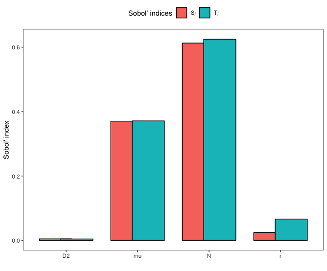
Figure 2: ** Preliminary results. First order $S_{i}$ and total effect $T_{i}$ Sobol indices of $1800$ model runs testing how variance in $D_{2}$, $\mu$, $N$ and $r$ translates to variance in the peak location of $I(x,t)$ at $t=7$ days. Sum of first order indices equals $1.012776$

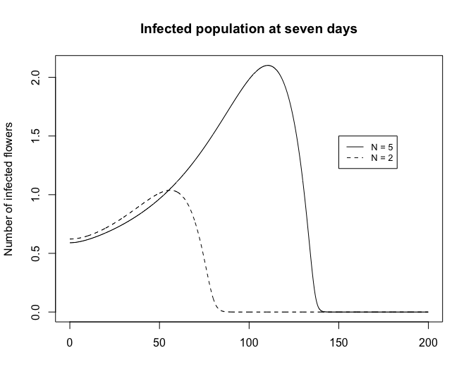
Figure 3: The curve $I(x,t)$ evaluated at seven days for two different values of $N$. All model parameters are taken from Table 5 with $r=0.5$, $\mu=0.5$ and $D_{2}=10$. Initial conditions were taken to be the same as in the sensitivity analysis, described at the start of section 4.2.

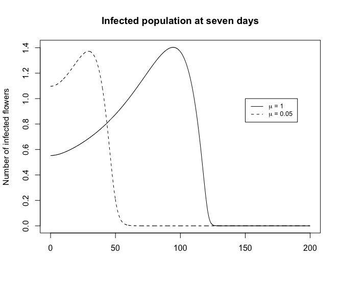
Figure 4: The curve $I(x,t)$ evaluated at seven days for two different values of $\mu$. All model parameters are taken from Table 5 with $r=0.5$, $N=3$ and $D_{2}=10$. Initial conditions were taken to be the same as in the sensitivity analysis, described at the start of section 4.2.

Table 4: Model parameters to be sampled using a uniform distribution.

Parameter	Symbol	Unit	Reference	Range
Diffusion coefficent for ooze-carry vectors	$D_{2}$	$m^{2}\cdot d^{-1}\cdot Fl.^{-1}$	Assumed	$[0,50]$
Visitation rate of ooze-carry vectors	$\mu$	$d^{-1}$	Assumed	$[0.05,1]$
Number of flowers in each cluster	$N$	Flowers	Assumed.	$[1,5]$
Growth rate of epiphytic pathogen population	$r$	$d^{-1}$	Assumed.	$[0.05,1]$

Table 5: Fixed model parameters and their values for the sensitivity analysis

Parameter	Symbol	Unit	Reference	Value
Diffusion coefficent for pollinating bees	$D_{1}$	$m^{2}\cdot d^{-1}$	Assumed	50
Carrying capacity of each living flower	$K$	CFUs $\cdot$ $\text{Fl.}^{-1}$.	[10,11]	$10^{6}$
Minimum carrying capacity of each cluster	$\epsilon$	CFUs	Assumed.	$10$
Decay rate of ooze	$\gamma$	$d^{-1}$	[15,16]	$0.0027$
Maximum infection rate	$M_{1}$	$d^{-1}$	Assumed	$1$
Maximum death rate	$M_{2}$	$d^{-1}$	Assumed	$1$
Ooze production rate	$\alpha$	CFUs  $\cdot$ $d^{-1}$ $\cdot$ $\text{Fl.}^{-1}$	[15]	$10^{8}$
Infection threshold	$A_{1}$	CFUs	Assumed	$10^{6}$
Death threshold	$A_{2}$	Fl.	Assumed	$1$
Infection rate Hill exponent	$n_{1}$	—	Assumed	$2$
Death rate Hill exponent	$n_{2}$	—	Assumed	$2$

Figure 2 and Figure 3 appear to suggest that blossom blight epidemics spread faster through high density orchards than through low density orchards. These results could be explained by the existence of a positive feedback loop between the pathogen and the number of infected flowers in an orchard, such that a greater amount of infected flowers produces a larger amount of the pathogen population in the form of ooze, which is disseminated and infects a larger number of flowers. It may seem from these results that one should not plant high-density orchards, however, the increased level of threat that diseases pose to high density orchards is something that growers are fully aware of. In fact, two of the more attractive features of planting high-density orchards is that the intra-tree competition causes the trees to grow more fruit and less wood or foliage, and that the management of such orchards is less labour-intensive due to the compact design. In the control of disease, these features are likely to make the implementation of IPM strategies more feasible, and allow spray programs to more evenly apply a pesticide. Then, although fire blight epidemics might move through high density orchards faster than traditionally planted ones, the potential increase in the efficiency of control measures could counter-act this difference.

The emergence of $\mu$ as an apparently significant parameter in the speed of disease spread, as displayed in Figure 2 and Figure 4, is especially interesting when compared to the growth rate of the epiphytic population $r$. Both of these parameters are sampled from identical ranges, and so one might expect that they would have similar effects on the speed of disease propagation. In fact, it seems natural to assume that the growth rate of the pathogen population would have the greater effect on the peak location, as the pathogen is fully capable of infection and dissemination without the presence of ooze. The observed results could be because the growth of the pathogen population due to $r$ is limited by the carrying capacity of the flowers, which is of the order of $10^{6}$ CFUs, whereas ooze is being released from infected flowers at a rate of $10^{8}$ CFUs per day, causing the deposit rate $\mu$ to significantly impact the pathogen population available for both infection and dissemination by bees. Then, it could be that the transfer of ooze from infected to susceptible flowers allows simultaneously for the high speed dissemination of the pathogen by bees as well as the infection of the susceptible flower.

It is important to note that we started with a large amount of the pathogen population already in the orchard. We suspect that starting with a much smaller pathogen population might change these results to highlight the significance of $r$, as this parameter is the only method by which the pathogen population grows prior to the infection of flowers and the release of ooze. It is very possible that $r$ would emerge as a more significant parameter in this study under different, but still realistic, initial conditions.

The parameter $D_{2}$ appears to have the least amount of impact, although it is important to note that we kept $D_{2}\leq D_{1}$ to keep the findings biologically relevant. The minimal impact of $D_{2}$ on the peak location of the infected wave has an interesting biological interpretation because it suggests that ooze-carrying vectors do not need high cluster-to-cluster mobility. This would imply that crawling insects could be just as responsible for a blossom blight outbreak as insects that fly, provided that they can transport ooze from locally infected flowers to locally susceptible flowers at a similar rate. This complicates the process of controlling ooze-carrying vectors, as one now needs to consider that multiple insect species, both flying and crawling, are playing a part in the spread of fire blight.

Lastly, there appears to be some connection between the results of Figure 2 and the minimum wave speed found in Theorem 3.3. If one assumed that the model parameters used in the sensitivity analysis resulted in travelling wave solutions, and that these waves travelled at the minimum wave speed of Theorem 3.3, then the results of the sensitivity analysis would seem almost trivial. The parameters $N$, $\mu$ and $r$ all explicitly appear in the formulation of this wave speed, and so one would expect that by sampling $N$ from a larger interval of larger values, this parameter would contribute a greater amount of variance to our model output of the peak location. This might also explain why $\mu$ has emerged as a more significant parameter than $r$ with regards to our model output, as $\mu$ is attached to $N$ in the formulation of the minimum wave speed whereas $r$ is not. Further, it is suspicious that $D_{2}$, the one parameter not present in our formulation of the minimum wave speed, appears to have the least significance in the speed of disease spread, despite being sampled from a much larger interval and being the only parameter in this experiment explicitly related to transport.

5 Discussion

5.1 The role of ooze and the control of blossom blight

Currently, the most common fire blight control strategy is to spray streptomycin repeatedly during bloom. Although generally effective, application of this pesticide is conditional on flowers being thoroughly covered, which can be problematic in low-density orchards with high foliage, and is also susceptible to the development of anti-bacterial resistant strains. In the case of both high and low density orchards, the results in Figure 2 and Figure 4 seem to emphasize the need for a control strategy that targets ooze carrying vectors. Although we only investigated blossom blight dynamics in a single growing season here, we expect that an extension of this model to include the overwintering and emergence of the pathogen via cankers would result in the same findings; that the transfer of ooze to susceptible flowers significantly increases the severity of a blossom blight epidemic. A hybrid control program consisting of both streptomycin applications and IPM strategies is likely to be the most effective and responsible approach to the control of fire blight in the years to come. However, there remains uncertainty over which insect species are responsible for the dissemination of ooze. Figure 2 seems to suggest that crawling insects could be just as responsible as flying insects when it comes to the dissemination of ooze, and given the large number of insect species naturally found in an orchard, it could be that multiple insect species are responsible for ooze dissemination and that the species most responsible for this mechanism changes geographically. This would suggest a need for further research into which insect species are capable of ooze transport, how these populations of insects change over time and which IPM strategies best control these insects.

In Figure 2 and Figure 3 we saw that blossom blight epidemics appear to move faster through high density orchards than low density orchards. This is probably due to a greater number of surfaces on which the pathogen can multiply, and a greater production of ooze when entire clusters are infected. However, in the context of control, one has to consider how the reduced foliage in high density orchards can lead to better coverage of a pesticide application. Although fire blight would seem to move faster through a high density orchard when left untreated, it could be that high density orchards allow for more effective disease control, both through a more targeted pesticide application and through less labour-intensive implementations of IPM strategies. Without investigating the effects and efficiency of the control methods in each orchard density type, it is hard to draw conclusions as to which is better for the management of fire blight, leaving us with many questions. What is an optimal approach to the management of fire blight? How might this change in high versus low density orchards? What are the costs versus benefits of certain IPM strategies for the control of fire blight in large-scale production settings? This lack of knowledge suggests a need for future work in fire blight modelling and in the field of optimal control for agricultural diseases.

5.2 Modelling fire blight in a spatial setting

In the first fire blight disease model [24], the authors assumed that pollinators move between trees in an orchard with equal probability, i.e, that the pollinator is just as likely to cross the entire orchard in the search for food as it is to travel to the neighbouring tree. In this paper, we make the assumption that the pollinators travel with equal probability between neighbouring trees. From this assumption, we derived a spatial model for the spread of blossom blight consisting of two reaction-diffusion equations coupled to a system of ordinary differential equations. Although we consider our assumption to be a more realistic one, it still faces an important limitation, in that it cannot model long distance flights by the pollinators or ooze-carrying vectors. A more realistic model would allow for vectors to make both short and long distance jumps between trees, which would seem more consistent with the observed flight patterns of orchard insects. It would be interesting to see what sort of disease dynamics arise when pollinators or ooze-carrying vectors follow a random walk in which the step sizes follow a Lévy distribution. Future experimental work, connecting the flight patterns of pollinators and ooze-carrying vectors, together with their behaviour in the presence of the pathogen population, would likely yield important insights into how, where and when blossom blight epidemics occur.

Another key difference between this work and the work in [24] is that we explicitly consider the production and dissemination of ooze. This led to the inclusion of a second PDE into our system. Often, coupled ODE-PDE models consist of a single PDE with a series of ODEs. The addition of this nonlinear PDE considerably increased the complexity of the analysis, in particular, when we searched for upper and lower solutions in the travelling wave proof. Further, there remains unanswered questions about the regularity of these solutions, and how this regularity might change depending on the initial conditions. Unfortunately, coupled ODE-PDE systems see significantly less attention in the literature, but are unavoidable if one wants to model the invasion of a disease into a population of stationary hosts. Another question that went answered here, but that is common amongst infectious disease models, is the stability of the disease-free equilibrium. We suspect that the disease-free equilibrium is unstable due to the underlying Fisher-KPP equation present in our model of the epiphytic pathogen population. In fact, it is easy to show that the disease free equilibrium is unstable in the ODE version of the system. However, this is far from conclusive. Although considerable work has been done in [65], in which a stability theorem for equilibrium solutions of a single reaction-diffusion equation coupled to a single ODE is presented, further work is needed to extend these results systems of multiple reaction-diffusion equations and ODEs so that plant disease modellers can more accurately describe the invasion of a pathogen into a field of crops.

5.3 Travelling waves, Schauder, upper and lower solutions

In Section 3, Theorem 3.3, we used Schauder’s fixed point theorem alongside the method of upper and lower solutions to prove that the coupled ODE-PDE system admits travelling wave solutions. This method is highly dependant on the ability to find appropriate upper and lower solutions, which is a formidable task when many non-linear functions are used in the model. The combination of Hill functions used in this model required us to impose conditions on the parameters in order to make the analysis feasible, which heavily restricted the set of parameters in which our proof covers. On top of this, the non-linearities in the PDE components made it difficult to find suitable upper and lower solutions, in which we circumvented this challenge by utilizing the existence of travelling waves in the Fisher-KPP equation. These challenges motivated us to study the solutions of our system when model parameters did not satisfy the constraints of Theorem 3.3. Combining the results of Theorem 3.3 with the results of section 4.1 gave us a much stronger belief that travelling wave solutions exist for model parameters outside of our proven range, indicating that these parameter constraints are sufficient conditions and not necessary ones for travelling waves to form in our system. However, it remains unclear whether the minimum wave speed of the theorem holds for larger sets of model parameters, as the results of section 4.1 appear to suggest that there are waves travelling slower than this speed for parameter sets that do not satisfy our constraints. We suspect that one could potentially prove the existence of travelling wave solutions for a broader range of model parameters than proven here, and derive a minimum wave speed that holds for all parameter choices. It would be interesting to see how a different approach to the proof, such as a shooting type argument, might lead to a more complete result, and what biological conclusions might be drawn from this.

6 Conclusion

In this study, we formulated and investigated a model for the spread of fire blight during bloom. By incorporating spatial effects, orchard density, and the production and dissemination of ooze, we were able to analyze the role that this symptom plays in how fast a blossom blight epidemic can propagate through both high and low density orchards.

Through analysis, we showed that under certain conditions the disease can move through an orchard in the form of a travelling wave, moving at a constant speed and maintaining a constant shape through space. Through numerical simulations, we found that the disease moves faster through high density orchards, and that the rate at which ooze-carrying vectors visit healthy flowers appears to play a significant role in the speed of spread. It could be that when ooze is transported onto the surface of healthy flowers, there is an abundant pathogen population available for both the infection of the flower and the high-speed dispersal of the pathogen by bees. The significant effect of this symptom on the global disease dynamics suggests two things, that models of fire blight should be analyzed in a spatial setting and that they should explicitly include both the production and dissemination of ooze.

References

1. Burrill, T. J. (1880). Anthrax of Fruit Trees: Or the So-called Fire Blight of Pear, and Twig Blight of Apple, Trees.

2. Denning, W. (1794). On the decay of apple trees. New York Society for the Promotion of Agricultural Arts and Manufacturers Transaction, 2, 219-222.

3. Van der Zwet, T., Orolaza-Halbrendt, N., Zeller, W. (2012). Spread and current distribution of fire blight. Fire blight: history, biology, and management, 15-36.

4. Makki, F. (2015). Review of Canadian Apple Market Trends. https://www.hortcouncil.ca/wp-693 content/uploads/2016/01/1-2015-AAFC-Presentation-on-Canadian-Apple-Situation-and-Trends-694 Midsummer-Apple-Industry-Meeting-Final-Version.pdf. PowerPoint Presentation

5. Ontario Apple Growers. (2016). Economic Impact of the Ontario Apple Industry.

6. Canadian Horticulture Council’s Apple Working Group. (2005). Fire Blight of Apple and Pear in Canada: Economic Importance and Strategy for Sustainable Management of the Disease.

7. Miller, P. W. (1929). Studies of fire blight of apple in Wisconsin. J. agric. Res, 39, 579-621.

8. Rosen, H. R. (1929). Life history of the fire blight pathogen, Bacillus amylovorus, as related to the means of over wintering and dissemination.

9. Thomson, S. V., Gouk, S. C. (2003). Influence of age of apple flowers on growth of Erwinia amylovora and biological control agents. Plant Disease, 87(5), 502-509.

10. Miller, T. D., Schroth, M. N. (1972). Monitoring the epiphytic population of Erwinia amylovora. Phytopathology, 62, 1175-1182.

11. Pusey, P. L., Curry, E. A. (2004). Temperature and pomaceous flower age related to colonization by Erwinia amylovora and antagonists. Phytopathology, 94(8), 901-911.

12. Rosen, H. R. (1936). Mode of penetration and of progressive invasion of fire-blight bacteria into apple and pear blossoms.

13. Thomson, S. V. (1986). The role of the stigma in fire blight infections. Phytopathology, 76(5), 476-482.

14. Slack, S. M., Zeng, Q., Outwater, C. A., Sundin, G. W. (2017). Microbiological examination of Erwinia amylovora exopolysaccharide ooze. Phytopathology, 107(4), 403-411.

15. Slack, S. M., Sundin, G. W. (2017). News on ooze, the fire blight spreader. Fruit Quarterly, 25(1), 9-12.

16. Hildebrand, E. M. (1939). Studies on fire blight ooze. Phytopathology, 29, 142-156.

17. Van der Zwet, T., Orolaza-Halbrendt, N., Zeller, W. (2012). The disease cycle of fire blight. Fire Blight Hist. Biol. Manag. American Phytopathological Society, St. Paul, MN, 155-182.

18. Boucher, M., Collins, R., Cox, K., Loeb, G. (2019). Effects of exposure time and biological state on acquisition and accumulation of Erwinia amylovora by Drosophila melanogaster. Applied and environmental microbiology, 85(15), e00726-19.

19. Kermack, W. O., McKendrick, A. G. (1927). A contribution to the mathematical theory of epidemics. Proceedings of the royal society of london. Series A, Containing papers of a mathematical and physical character, 115(772), 700-721.

20. Segarra, J., Jeger, M. J., Van den Bosch, F. (2001). Epidemic dynamics and patterns of plant diseases. Phytopathology, 91(10), 1001-1010.

21. Jeger, M. J., Van den Bosch, F., Madden, L. V. (2011). Modelling virus-and host-limitation in vectored plant disease epidemics. Virus research, 159(2), 215-222.

22. Bokil, V. A., Allen, L. J. S., Jeger, M. J., Lenhart, S. (2019). Optimal control of a vectored plant disease model for a crop with continuous replanting. Journal of biological dynamics, 13(sup1), 325-353.

23. Hamelin, F. M., Bowen, B., Bernhard, P., Bokil, V. A. (2021). Optimal control of plant disease epidemics with clean seed usage. Bulletin of Mathematical Biology, 83(5), 1-24.

24. Iljon, T., Stirling, J., Smith?, R. J. (2012). A mathematical model describing an outbreak of fire blight. Understanding the Dynamics of Emerging and Re-Emerging Infectious Diseases Using Mathematical Models.

25. Steiner, P. W. (1989, June). Predicting canker, shoot and trauma blight phases of apple fire blight epidemics using the MARYBLYT model. In V International Workshop on Fire Blight 273 (pp. 149-158).

26. Lightner, G. W., Steiner, P. W. (1992). Maryblyt™: a computer model for predicting of fire blight disease in apples and pears. Computers and electronics in agriculture, 7(3), 249-260.

27. Smith, T. J. (1998, October). REPORT ON THE DEVELOPMENT AND USE OF COUGARBLIGHT 98C-A SITUATION-SPECIFIC FIRE BLIGHT RISK ASSESSMENT MODEL FOR APPLE AND PEAR. In VIII International Workshop on Fire Blight 489 (pp. 429-436).

28. Smith, T. J., Pusey, P. L. (2010, August). CougarBlight 2010, a significant update of the CougarBlight fire blight infection risk model. In XII International Workshop on Fire Blight 896 (pp. 331-336).

29. Burie, J. B., Calonnec, A., Langlais, M. (2008). Modeling of the invasion of a fungal disease over a vineyard. In Mathematical Modeling of Biological Systems, Volume II (pp. 11-21). Birkhäuser Boston.

30. Atallah, S. S., Gómez, M. I., Conrad, J. M., Nyrop, J. P. (2015). A Plant‐Level, Spatial, Bioeconomic Model of Plant Disease Diffusion and Control: Grapevine Leafroll Disease. American Journal of Agricultural Economics, 97(1), 199-218.

31. Bolker, B. M. (1999). Analytic models for the patchy spread of plant disease. Bulletin of mathematical biology, 61(5), 849-874.

32. Madden, L. V., Hughes, G., Van Den Bosch, F. (2007). The study of plant disease epidemics.

33. Schoofs, H., Delalieux, S., Deckers, T., Bylemans, D. (2020). Fire Blight Monitoring in Pear Orchards by Unmanned Airborne Vehicles (UAV) Systems Carrying Spectral Sensors. Agronomy, 10(5), 615.

34. Sanchirico, J. N., Wilen, J. E. (2005). Optimal spatial management of renewable resources: matching policy scope to ecosystem scale. Journal of Environmental Economics and Management, 50(1), 23-46.

35. Thomson, S. V., Gouk, S. C., Vanneste, J. L., Hale, C. N., Clark, R. G. (1992, October). The presence of streptomycin resistant strains of Erwinia amylovora in New Zealand. In VI International Workshop on Fire Blight 338 (pp. 223-230).

36. El‐Goorani, M. A., El‐Kasheir, H. M. (1989). Distribution of streptomycin resistant strains of Erwinia amylovora and control of fire blight disease in Egypt. Journal of Phytopathology, 124(2), 137-142.

37. IPM Institute of North America what is Integrated Pest Management? IPM Institute of North America. (n.d.). Retrieved January 2, 2022, from https://ipminstitute.org/what-is-integrated-pest-management/ .

38. Chen, C., Li, C., Kang, Y. (2018). Modelling the effects of cutting off infected branches and replanting on fire-blight transmission using Filippov systems. Journal of theoretical biology, 439, 127-140.

39. Burrill, A. C. (1915). Insect control important in checking fire blight. Phytopathology, 5, 343-347.

40. Joshi, N. K., Ngugi, H. K., Biddinger, D. J. (2020). Bee Vectoring: Development of the Japanese Orchard Bee as a Targeted Delivery System of Biological Control Agents for Fire Blight Management. Pathogens, 9(1), 41.

41. Okubo, A., Levin, S. A. (2001). Diffusion and ecological problems: modern perspectives (Vol. 14, pp. xx+-467). New York: Springer.

42. Webb, G. F. (1981). A reaction-diffusion model for a deterministic diffusive epidemic. Journal of Mathematical Analysis and Applications, 84(1), 150-161.

43. Wilson, R. E., Capasso, V. (1997). Analysis of a Reaction-Diffusion System Modeling Man–Environment–Man Epidemics. SIAM Journal on Applied Mathematics, 57(2), 327-346.

44. Wang, W., Zhao, X. Q. (2012). Basic reproduction numbers for reaction-diffusion epidemic models. SIAM Journal on Applied Dynamical Systems, 11(4), 1652-1673.

45. Ai, S. (2010). Traveling waves for a model of a fungal disease over a vineyard. SIAM journal on mathematical analysis, 42(2), 833-856.

46. Fu, S. C. (2016). Traveling waves for a diffusive SIR model with delay. Journal of Mathematical Analysis and Applications, 435(1), 20-37.

47. Mischaikow, K., Reineck, J. F. (1993). Travelling waves in predator-prey systems. SIAM journal on mathematical analysis, 24(5), 1179-1214.

48. Fisher, R. A. (1937). The wave of advance of advantageous genes. Annals of eugenics, 7(4), 355-369.

49. Kolmogorov, A. N. (1937). A study of the equation of diffusion with increase in the quantity of matter, and its application to a biological problem. Moscow University Bulletin of Mathematics, 1, 1-25.

50. Volpert, A. I., Volpert, V. A., Volpert, V. A. (1995). Traveling wave solutions of parabolic systems. Bull. Amer. Math. Soc, 32, 446-452.

51. Dunbar, S. R. (1983). Travelling wave solutions of diffusive Lotka-Volterra equations. Journal of Mathematical Biology, 17(1), 11-32.

52. Ma, S. (2001). Traveling wavefronts for delayed reaction-diffusion systems via a fixed point theorem. Journal of Differential Equations, 171(2), 294-314.

53. Huang, J. H., Zou, X. F. (2006). Travelling wave solutions in delayed reaction diffusion systems with partial monotonicity. Acta Mathematicae Applicatae Sinica, 22(2), 243-256.

54. Shu, H., Pan, X., Wang, X. S., Wu, J. (2019). Traveling waves in epidemic models: non-monotone diffusive systems with non-monotone incidence rates. Journal of Dynamics and Differential Equations, 31(2), 883-901.

55. Shang, X., Du, Z., Lin, X. (2016). Traveling wave solutions of n‐dimensional delayed reaction–diffusion systems and application to four‐dimensional predator–prey systems. Mathematical Methods in the Applied Sciences, 39(6), 1607-1620.

56. Zhou, J., Song, L., Wei, J., Xu, H. (2019). Critical traveling waves in a diffusive disease model. Journal of Mathematical Analysis and Applications, 476(2), 522-538.

57. Smoller, J. (2012). Shock waves and reaction—diffusion equations (Vol. 258). Springer Science & Business Media.

58. Logan, J. D. (2008). An introduction to nonlinear partial differential equations (Vol. 89). John Wiley & Sons.

59. Wang, X. S., Wang, H., Wu, J. (2012). Traveling waves of diffusive predator-prey systems: disease outbreak propagation. Discrete & Continuous Dynamical Systems, 32(9), 3303.

60. Wang, H., Wang, X. S. (2016). Traveling wave phenomena in a Kermack–McKendrick SIR model. Journal of Dynamics and Differential Equations, 28(1), 143-166.

61. Puy, A., Piano, S. L., Saltelli, A., Levin, S. A. (2021). sensobol: an R package to compute variance-based sensitivity indices. arXiv preprint arXiv:2101.10103.

62. Soetaert, K., Petzoldt, T., Setzer, R. W. (2010). Solving differential equations in R: package deSolve. Journal of statistical software, 33, 1-25.

63. Saltelli, A., Annoni, P., Azzini, I., Campolongo, F., Ratto, M., Tarantola, S. (2010). Variance based sensitivity analysis of model output. Design and estimator for the total sensitivity index. Computer physics communications, 181(2), 259-270.

64. Jansen, M. J. (1999). Analysis of variance designs for model output. Computer Physics Communications, 117(1-2), 35-43.

65. Marciniak-Czochra, A., Karch, G., Suzuki, K. (2017). Instability of Turing patterns in reaction-diffusion-ODE systems. Journal of mathematical biology, 74(3), 583-618.