A hybrid adaptive multiresolution approach for the efficient simulation of reactive flows

Abstract

Computational studies that use block-structured adaptive mesh refinement (AMR) approaches suffer from unnecessarily high mesh resolution in regions adjacent to important solution features. This deficiency limits the performance of AMR codes. In this work a novel hybrid adaptive multiresolution (HAMR) approach to AMR-based calculations is introduced to address this issue. The multiresolution (MR) smoothness indicators are used to identify regions of smoothness on the mesh where the computational cost of individual physics solvers may be decreased by replacing direct calculations with interpolation. We suggest an approach to balance the errors due to the adaptive discretization and the interpolation of physics quantities such that the overall accuracy of the HAMR solution is consistent with that of the MR-driven AMR solution. The performance of the HAMR scheme is evaluated for a range of test problems, from pure hydrodynamics to turbulent combustion.

1 Introduction

Combustion is a physical process that plays a critical role in many industrial, defense, and basic science applications. Oftentimes combustion is accompanied by the chaotic mixing process known as turbulence. These phenomena are prevalent in problems ranging from internal combustion engines to stellar evolution. Significant progress has been made in the numerical modeling of such processes (c.f. [1]). However, as the physics models used to describe turbulent combustion become increasingly complex, the need for more efficient computational tools increases commensurately.

One of the major challenges associated with simulations of turbulent combustion is the presence of disparate length and time scales. In particular, the thermonuclear burning timescale in the problem of detonation ignition and turbulent stellar plasma [2] is on the order of $\tau_{\mathrm{burn}}\approx 1\times 10^{-9}$ s, whereas the eddy turnover time is $\tau_{\mathrm{turb}}\approx 1\times 10^{-2}$ s. At the same time, the turbulent kinetic energy transfer couples the turbulence driving scales, $l_{\mathrm{td}}\approx 1\times 10^{6}$ cm, with the viscous dissipation scale, which is several orders of magnitude smaller. This disparity in scales frequently makes direct numerical simulations computationally infeasible, forcing researchers to reduce the range of scales by introducing approximate descriptions of physics operating on unresolvable scales [3]. The above situation might be further complicated by the contribution of additional effects such as compressibility (due to coupling to burning) and anisotropy (due to gravity). In the case of compressibility, provided that the resulting energy release is sufficiently high, acoustic perturbations might be strengthened into shocks and ultimately become detonation waves [4]. The reaction zones supporting detonations not only see extreme changes in internal energy, but are also small in comparison to the size of the computational domain. Furthermore, the physical description of the participating medium requires in this case the use of a complex stellar equation of state (EOS). This type of EoS is very costly to evaluate in comparison to hydrodynamics [5].

The above problem description indicates that accurately resolving turbulence and reactive scales may not be possible when using a uniform spatial resolution. One class of numerical discretization algorithms designed to address the challenge of disparate scales are adaptive mesh refinement (AMR) methods. These methods employ a hierarchical approach to progressively resolve solution structure, with the refinement process being driven by relevant mesh refinement criteria. These criteria are of key importance in achieving the required solution accuracy at minimal computational cost. To adapt the mesh, Berger & Oliger [6] used Richardson extrapolation to estimate the local truncation error (LTE) of the solution. Because the solution error is expected to depend on the amount of variation in the solution, less sophisticated methods that rely on the first-order solution variation [7], or possibly higher-order derivatives [8] have been used for that purpose. In certain situations it might be useful to drive mesh refinement using application-specific refinement criteria, such as abundance or rate of mixing of reactive species. (For a partial review of the LTE estimators and other refinement criteria, as well as an analysis of AMR solution error for certain classes of partial differential equations (PDEs), see [9].)

Alternative approaches to dynamically adaptive schemes based on multiresolution analysis (MRA) have gained popularity in the computational fluid dynamics community over the last two decades [10]. MRA provides a mathematically rigorous setting for the representation of discrete data in terms of nested approximation spaces, and serves as the basis of multiresolution (MR) adaptive techniques for solving PDEs [11]. The seminal papers by Harten [12, 13] introduced a MR scheme for solving hyperbolic conservation laws (HCLs) that reduces computational expense by adaptively computing the numerical flux. In Harten’s scheme, the MR indicators are used to identify solution regions of sufficient smoothness where costly, high resolution numerical fluxes do not need to be computed directly to achieve the desired accuracy. Instead those fluxes are interpolated using high resolution flux values already obtained nearby. In contrast to AMR methods, Harten’s scheme evolves the solution uniformly at the finest level of mesh resolution.

Initially, Harten’s scheme was applied solely to the Euler equations in one spatial dimension, but was then extended by Bihari et al. to include viscous effects [14], to two-dimensional situations [15], and also to PDEs with reactive source terms [16]. The same principle was also used by Chiavassa & Donat [17] to accelerate the computation of solutions to the multidimensional Euler equations. We refer to this class of MR schemes as solver adaptive.

Although Harten’s intent was to offer an algorithmically simpler alternative to grid adaptation [13], the adaptive mesh setting was eventually used with the MR framework by Gottschlich-Müller & Müller [18] to construct a fully adaptive MR scheme (see, also, [19]). Cohen et al. [20] also introduced a fully adaptive MR scheme for multidimensional HCLs, and provided rigorous error analysis. Roussel and collaborators used MR indicators to guide mesh adaptation for solving parabolic PDEs in [21] and the reactive Euler equations in [22, 23]. Domingues et al. [24, 25] combined this approach with locally adaptive time-stepping schemes. Generally speaking, these works employ AMR with the refinement criteria determined by the MR smoothness indicators.

In regard to the AMR mesh structure, it can be described as a collection of individual cells (cell-based format; [26]), blocks containing a fixed number of cells (block-based, or block-structured format; [27]), or blocks containing varying number of cells (patch-based format; [6]). The efficiency of those various discretizations can be characterized using the mesh filling factor, which is the ratio of the number of cells required to resolve the solution in the AMR model to the number of cells in the corresponding uniformly resolved model. This mesh filling factor is the smallest possible for cell-based refinement, but usually higher for the latter two formats. However block- and patch-based formats are generally better suited for large distributed memory machines due to lower network communication costs (see, for example, [28, 29, 30]). The choice of which AMR discretization format to use depends on the computing hardware and application type.

Many libraries implementing the patch- or block-based AMR approaches are available. For example in our work we use the block-based PARAMESH library as implemented in the flash code [31]. As mentioned earlier this approach allows for relatively simple mesh management with little associated metadata, and for simple physics applications scales well for problems requiring thousands of processors [32]. The patch-based format is offered in numerous AMR libraries, including BoxLib/AMReX [33, 34], SAMRAI [35], AMROC [36], and Chombo [37], among others. Compared to the block-based format the patch-based refinement calculations may require more extensive metadata and more complex communication patterns, which may negatively impact load balancing in large-scale simulations. For these reasons, optimization of patch-based AMR algorithms remains an active area of research [28, 38].

Recently, MR approaches have been combined with block-structured AMR. For example, Han et al. [39] employ a block-structured multiresolution adaptive approach for simulating multi-phase flows, with the blocks being organized in a pyramid-like data structure that allows overlap between neighbors. Sroka et al. [40] introduced a finite-difference based, open-source, block-structured MR-driven AMR code. Deiterding et al. [41] showed the benefits of using MR indicators in the AMROC code for several multi-dimensional test problems. The trend of MR schemes towards either patch- or block-based AMR can be understood as preference for more efficient memory access patterns and scalable computing. However, the mesh efficiency issues often present with these AMR formats has yet to be sufficiently addressed.

In the current work, we present a hybrid adaptive MR (HAMR) approach that combines the scalability of block-structured AMR with the potential efficiency increase offered by the solver adaptive approach. This scheme uses MR indicators not only to adapt the mesh, but also to identify solution regions where otherwise costly computations involving various physics can be replaced safely with interpolation without sacrificing the overall solution accuracy. We apply the solver adaptive approach to the hydrodynamic fluxes as well as to composite functions of the solution, in particular the reactive source term and the EoS. Although we demonstrate this approach in the context of compressible reactive turbulence, other physics solvers can be treated in the same way. We use several benchmark problems to evaluate computational cost savings.

The paper is organized as follows. In section 2 we introduce the system of coupled, nonlinear PDEs that are the subject of our investigation, as well as the finite volume (FV) scheme used to numerically solve those equations. We also provide an overview of the basics of MR adaptive schemes. In section 3, we present the HAMR scheme, which uses MR smoothness indicators not only to adapt the mesh but also to reduce the computational cost of the physics solvers. We apply the new scheme to select problems in section 4, and in section 5 we provide analysis in terms of solution accuracy and overall computational efficiency.

2 Preliminaries

We begin our presentation by defining the basic components of the new scheme, including the model PDEs, FV framework, and the MR background.

2.1 Reactive flow equations

The present approach is concerned with numerically solving the Euler equations for compressible, reactive flows:

$$\rho_{t}+\nabla\cdot(\rho\bm{v}) =0,$$ (1a)

$$(\rho\bm{v})_{t}+\nabla\cdot(\rho\bm{v}\bm{v}^{T}+p\bm{I}) =\bm{0},$$ (1b)

$$(\rho\bm{X})_{t}+\nabla\cdot\left(\rho\bm{X}\bm{v}\right) =\bm{R},$$ (1c)

$$(\rho E)_{t}+\nabla\cdot\left(\rho E+p\right)\bm{v} =\dot{Q}.$$ (1d)

Here $\rho$ is the mass density of the gas mixture, $\bm{v}$ is the velocity vector, $p$ is the pressure, $E$ is the specific total energy, $\bm{X}$ is the vector of species mass fractions, $\bm{R}$ is the vector of species reaction rates, and $\dot{Q}$ is the energy source term. The mass fraction for the $i^{\mathrm{th}}$ species can be written as $X_{i}=\rho_{i}/\rho$, where $\rho_{i}$ is the corresponding mass density, meaning that the species must collectively satisfy the constraint $\sum_{i=1}^{\mathcal{N}_{\mathrm{species}}}X_{i}=1$, where $\mathcal{N}_{\mathrm{species}}$ is the number of species considered.

The total specific energy is calculated as the sum of the specific internal energy and the kinetic energy as $E=e+\frac{1}{2}\bm{v}\bm{v}^{T}$. The above system of PDEs is closed using a suitable EoS which relates the pressure to density, internal energy, and composition (see below and section 3.3).

2.2 Finite volume method

The equations 1 are discretized using the standard FV approach. Given a uniform discretization of the domain $x\in[x_{a},x_{b}]$ with cell size $h=(x_{b}-x_{a})/N$, where $N$ is the number of cells, the following semi-discrete scheme is considered:

$$u_{i}^{n+1}=u_{i}^{n}-\frac{1}{h}\int_{t_{n}}^{t_{n+1}}\left(\hat{f}_{i}-\hat{f}_{i-1}\right)dt+\int_{t_{n}}^{t_{n+1}}\hat{s}_{i}dt.$$ (2)

Here, $u_{i}^{n}$ is an approximation to the average of the exact solution, which we denote as $q(x,t)$, in the control volume $[x_{i-1},x_{i}]$ at $t_{n}$. The numerical flux approximates the exact flux function as

$$\hat{f}_{i}\coloneqq\hat{f}\left(u_{i-k},\dots,u_{i+k+1}\right)\approx f\left(q(x_{i},t)\right),$$ (3)

where $2k$ is the number of cells comprising the reconstruction stencil. Likewise, the term

$$\hat{s}_{i}\coloneqq s(u_{i})\approx\frac{1}{h}\int_{x_{i-1}}^{x_{i}}s(q(x,t))dx$$ (4)

is an approximate average of the exact source term within the control volume. We present these equations in the semi-discrete form to emphasize that the fluxes and source terms can be handled separately in time using standard operator splitting approaches (see, [42], and references therein).

2.3 Multiresolution decomposition

The MR representation has been used for the purpose of dynamic mesh adaptation in a number of FV-based approaches. These approaches rely on the local MR smoothness indicators to adapt the mesh. The smoothness indicators are obtained on a hierarchy of nested meshes. We outline the MR decomposition presented in [12], which is appropriate for the current one-dimensional presentation, and refer the reader to [15] and [21] for the two- and three-dimensional extensions, respectively. The mesh hierarchy is defined as

$$\bm{\mathcal{G}}_{l}=\left\{x_{l,i}\right\}_{i=0}^{N_{l}},\quad x_{l,i}=x_{a}+i\cdot h_{l},\quad h_{l}=2^{(L-l)}h_{L},\quad N_{l}=N_{L}/2^{(L-l)},$$ (5)

where $L$ is the finest level of mesh resolution allowed and $1\leq l\leq L$. The objective in introducing 5 is to represent the fine-grid data as a sum of data averages on the coarsest level plus a series of differences defined on finer levels. Given cell averages on the finest level of resolution, $\bm{u}^{n}_{L}=\left\{u_{L,i}^{n}\right\}_{i=1}^{N_{L}}$, where $n$ is the time index, the decomposition is performed using the following set of mappings beginning with level $l=L-1$ and ending with level $l=1$. First, cells on level $l+1$ are projected onto the coarser grid level $l$ by means of volume weighted averaging. Then, approximate cell averages on the finer level $l+1$ are predicted by an average-interpolating polynomial constructed with data on level $l$. In this work we use the third-order polynomial commonly found in the literature.

The smoothness of the data is assessed using detail coefficients. These coefficients are computed as the difference between actual and predicted values as

$$d_{l,i}^{n}=u_{l+1,2i}^{n}-\tilde{u}_{l+1,2i}^{n},$$ (6)

where $\tilde{u}_{l+1,2i}$ is the prediction based on coarser data (see [12] for one-dimensional formulae). The detail coefficients are a measure of the local regularity of the solution, and their values decay in relation to that solution regularity as the mesh resolution increases [12].

Compression of the MR representation is achieved by simply setting to zero the coefficients whose magnitudes are below a prescribed threshold. In this work we adopt the scale dependent threshold of Harten, $\varepsilon_{l}=\varepsilon/2^{\left(L-l\right)}$, where $\varepsilon$ ($=\varepsilon_{L}$) is the prescribed tolerance. The remaining non-zero detail coefficients form a set of significant detail coefficients and encode the information necessary to approximate the fine-grid data to a prescribed level of accuracy. This set of significant detail coefficients is given by $\bm{\mathcal{D}}^{n}=\left\{(l,i)\mathrel{\mathop{\mathchar 58\relax}}\ |d^{n}_{l,i}|>\varepsilon_{l}\right\}$.

Due to the time-dependent character of the solution, the set of cells determined to be significant at a given time will in general be inadequate for describing future states. In the case of the CFL-limited time step integration, the solution structure evolves slowly with a rate of at most one cell per step. Thus one can safely assume that the MR decomposition will correctly capture relevant solution structures at future times by anticipating the amount of variation in the neighborhood [12, 20].

To maintain a reliable MR representation, the set $\bm{\mathcal{D}}^{n}$ is extended to include coefficients that belong to the a priori unknown set $\bm{\mathcal{D}}^{n+1}$ as well. Thus a prediction set $\tilde{\bm{\mathcal{D}}}^{n+1}$ is created with the intent of satisfying the condition,

$$\bm{\mathcal{D}}^{n}\cup\bm{\mathcal{D}}^{n+1}\subset\tilde{\bm{\mathcal{D}}}^{n+1}.$$ (7)

The set $\tilde{\bm{\mathcal{D}}}^{n+1}$ can be estimated by constructing a mask, $\bm{\mathcal{M}}^{n}$, initially set to $\bm{\mathcal{D}}^{n}$ and then expanded by adding a buffer region such that

$$\bm{\mathcal{M}}^{n}\coloneqq\bm{\mathcal{D}}^{n}\cup\left\{(l,i)\mathrel{\mathop{\mathchar 58\relax}}|i-\hat{\imath}|\leq\mathcal{N}_{\mathrm{buffer}}\right\},$$ (8)

where $\mathcal{N}_{\mathrm{buffer}}$ is the size of the buffer region and $(l,\hat{\imath})\in\bm{\mathcal{D}}^{n}$. For added reliability of the MR scheme, more cells can be included in the buffer region to account for possible rapid development of the solution structure [12, 20].

As alluded to earlier in this section, the buffer size in practical applications is determined by the numerical speed of signal propagation on the mesh. For HCLs, this constraint is expressed by the usual CFL condition [43]. For that reason, if the MR decomposition is performed at every timestep, then the minimal buffer size required to satisfy the reliability condition 7 should be $\mathcal{N}_{\mathrm{buffer}}=1$. If one wishes to refine less often, then the buffer size should be proportionally increased.

3 Hybrid adaptive multiresolution scheme

In this section we introduce the proposed HAMR scheme, which combines the MR-driven block-structured AMR with the solver-adaptive ideas initially proposed by Harten [12]. To describe this approach we must consider the reference FV scheme 2 on the MR hierarchy 5. The MR FV scheme is defined on each level $l$ of the hierarchy as,

$$u^{*}_{l,i} =u^{n}_{l,i}-\frac{\Delta t}{h_{l}}\left(\bar{f}_{l,i}-\bar{f}_{l,i-1}\right),$$ (9a)

$$u^{n+1}_{l,i} =u^{*}_{l,i}+\Delta t\hat{s}^{n+1}_{l,i},$$ (9b)

where $i=1,\dots,N_{l}$ and $\bar{f}_{l,i}$ is the time-averaged numerical flux through the respective interface. Here we utilize the Godunov operator splitting approach [44], with the reactive source terms being treated implicitly . The question of how to compute the fluxes and sources on the adaptive hierarchy is briefly reviewed. We summarize three main approaches available in the literature, and then describe how the new HAMR scheme operates.

The first approach, pioneered by Harten [12] and which we refer to as solver adaptive, evolves the numerical solution on the finest mesh level but reduces computational effort in smooth regions by replacing direct flux calculations with interpolation from values previously computed on coarser levels. The fluxes on coarse levels are computed as

$$\bar{f}_{l,i}=\bar{f}\left(\tilde{u}_{L,2^{L-l}i-k+1}^{n},\dots,\tilde{u}_{L,2^{L-l}i+k}^{n}\right).$$ (10)

Here $2^{L-l}i$ is the index corresponding to interface $i$ on the coarse level, as represented on the finest level, $L$. The MR-interpolated solution, $\tilde{\bm{u}}_{L}^{n}$, is obtained via the inverse MR decomposition based on the significant set of cells $\bm{\mathcal{M}}^{n}$ (note that in this approach, the inverse MR decomposition needs only to be considered for analysis purposes, as the fine-scale solution data is always available). In a closely related work involving reactive systems, Bihari & Harten [16] also evaluate source terms (explicitly) as a function of fine-scale data as

$$\hat{s}_{l,i}^{n}=\frac{1}{2^{L-l}}\sum_{\hat{\imath}=1}^{2^{L-l}}\hat{s}_{L,2^{L-l}(i-1)+\hat{\imath}}^{n}.$$ (11)

Naturally this approach has the inherent disadvantage of the computational complexity being dependent on the finest mesh level.

The second type of approach, initially developed by Gottschlich-Müller & Müller [18] and Cohen et al. [20], contrasts with the approach of Harten by introducing an adaptive, nonuniform discretization based on the MR indicators. In this approach, 10 is used in conjunction with the inverse MR decomposition to compute coarse-scale fluxes as a function of fine-scale data in order to avoid the discretization error associated with the local level of resolution. This type of procedure is referred to as the exact local reconstruction. A variation of this approach, explored by Hovhannisyan & Müller [45] and referred to as the approximate reconstruction strategy, utilizes an interpolating polynomial constructed from local averages in conjunction with an appropriate quadruate rule to reduce the computational complexity while maintaining accuracy.

The third, simplest and most commonly used strategy of handling fluxes and source terms on the adaptive mesh is to provide the solvers with local solution averages. This direct evaluation strategy is attractive because it has the lowest computational complexity. However, it is expected to incur the greatest overall error – this is because the contributing discretization error is set by the local resolution (which might be coarser than the finest allowed resolution), while in the other two approaches described above, the error is always set by the finest allowed mesh resolution (by using interpolation procedures).

The HAMR approach developed in this work adapts the block-structured mesh according to the MR mask 8, and employs a hybrid strategy for the evaluation of fluxes and composite functions on each individual mesh block. Principally, the evolution of the solution on each mesh block is handled according to the direct evaluation strategy. However, computations are further accelerated locally by the use of the solver adaptive approach. In particular, the fluxes are computed in the same fashion as Harten’s original approach, but in this case the flux formula 10 is applied with respect to the block’s level, $l$, rather than the finest level, $L$. Composite functions are treated similarly.

Our description now turns to the construction of the adaptive mesh and the procedure for adaptively computing fluxes and composite functions on that mesh.

3.1 Block-structured adaptive mesh refinement

We consider dynamically adaptive block-structured mesh hierarchies. For such a mesh hierarchy, the natural data representation is a tree-like structure (binary tree, quadtree, or octree in one, two, or three dimensions, respectively). The blocks in the hierarchy each consist of a fixed number of computational cells, $N_{\mathrm{c}}$ in each dimension, and the block refinement produces $2^{d}$ children blocks, where $d$ is the number of dimensions. The numerical solution is obtained and evolved on blocks that are no further refined, referred to as leaf blocks. In addition to the computational cells, blocks must be equipped with ghost cells to provide the PDE solvers with data beyond the block boundaries necessary for operations using long data stencils.

3.1.1 Local MR hierarchy

We decompose the global MR hierarchy (spanning the computational domain) into a collection of local MR hierarchies, with each leaf block being assigned a partition of the global hierarchy in space and in scale. Each leaf block serves the dual purpose of handling a part of the solution and a respective part of the MR decomposition. On each leaf block there are $\mathcal{L}$ levels defined, with the finest level corresponding to the block’s global MR (or AMR) level.

The number of levels existing in the local MR hierarchy is limited by the number of cells in the block, $N_{\mathrm{c}}$ ($=N_{\mathcal{L}}$) as well as the extent of the ghost region ($N_{\mathrm{gc}}$ cells in each direction). The latter limitation is due to the number of cells required by the prediction operator stencil. As the local MR hierarchy depth increases, more cells are required from neighboring blocks to supply boundary data for the stencils. This situation is illustrated in fig. 1,

Figure 1: The local MR hierarchy on the AMR leaf block, with $N_{\mathrm{gc}}=4$ ghost cells on each end, and the block having $N_{\mathrm{c}}=16$ cells. Dependencies for the one-dimensional, third-order prediction operator are shown near the boundaries, illustrating the need for ghost cells (colored in gray), and the limit on the number of levels that can be handled. At most three levels can be handled in this case.

where we show the local MR hierarchy for a given block, interpolation dependencies at the block’s boundaries, and block ghost cell regions. Although the figure illustrates the situation in one dimension, the same dependencies carry over in the multi-dimensional case.

3.1.2 MR mask and block refinement and coarsening

The MR decomposition is computed on each local MR hierarchy as follows. Let $\bm{\mathcal{B}}^{n}$ denote the set of AMR leaf block IDs at timestep $n$, and let $\bm{\mathcal{M}}^{n}_{b}$ denote a component of the MR mask defined by 8, where $b\in\bm{\mathcal{B}}^{n}$. One can define for each leaf block $b$ a local-to-global mapping operator that maps the local hierarchy index space to the global hierarchy index space as $\mathcal{T}_{b}\mathrel{\mathop{\mathchar 58\relax}}\bm{\mathcal{M}}^{n}_{b}\mapsto\bm{\mathcal{M}}^{n}$. The global MR mask can then be formed via the union of local masks as

$$\bigcup_{b\in\bm{\mathcal{B}}^{n}}\mathcal{T}_{b}\left(\bm{\mathcal{M}}^{n}_{b}\right)\subset\bm{\mathcal{M}}^{n}.$$ (12)

We note that while the MR decomposition performed on the local MR hierarchies produces a subset of the mask that would be obtained by performing the complete decomposition, the union of local masks is actually sufficient for the purpose of adapting the mesh. This is because the elements missing from the union of local masks correspond to cells belonging to inactive AMR (parent) blocks, and are not useful for mesh adaptation.

Flagging for refinement or coarsening for block $b$ is done according to the following rules:

1. if there exists any $(\mathcal{L}-1,i)\in\bm{\mathcal{M}}_{b}^{n}$,

2. if there does not exist any $(\mathcal{L}-2,i)\in\bm{\mathcal{M}}_{b}^{n}$.

Note that we keep one finer mesh level than is otherwise indicated by the detail coefficients in order to capture any fine-scale information that might emerge during time integration.

3.2 Adaptive calculation of fluxes on the local MR hierarchy

The computation of numerical fluxes on the local MR hierarchy follows the procedure outlined in [12]. That is, the MR mask is used to identify interfaces where the flux may be accurately interpolated from values already obtained at interfaces corresponding to coarser grid levels.

On the local MR hierarchy, the fluxes, when calculated directly, are calculated according to 10 but with level $L$ being replaced by $\mathcal{L}$. This is consistent with the direct evaluation strategy discussed in section 3. Further savings are introduced by interpolating fluxes at odd-indexed interfaces according to the MR mask. Flux values at level $l+1$ may be interpolated in a pointwise sense from values obtained on level $l$ using

$$\bar{f}_{l+1,2i-1}\approx I_{r}(l,i;\bm{\bar{f}}_{l}),$$ (13)

where

$$I_{r=0}(l,i;\bm{\bar{f}}_{l}) \coloneqq\frac{1}{2}(\bar{f}_{l,i-1}+\bar{f}_{l,i}),\quad i=1,\dots,N_{l},$$ (14a)

$$I_{r=1}(l,i;\bm{\bar{f}}_{l}) \coloneqq\begin{cases}\frac{1}{16}(5\bar{f}_{l,i-1}+15\bar{f}_{l,i}-5\bar{f}_{l,i+1}+\bar{f}_{l,i+2}),&i=1,\\ \frac{1}{16}(-\bar{f}_{l,i-2}+9\bar{f}_{l,i-1}+9\bar{f}_{l,i}-\bar{f}_{l,i+1}),&i=2,\dots,N_{l}-1,\\ \frac{1}{16}(\bar{f}_{l,i-3}-5\bar{f}_{l,i-2}+15\bar{f}_{l,i-1}+5\bar{f}_{l,i}),&i=N_{l}.\end{cases}$$ (14b)

Here, the order of accuracy of the interpolation is $2r+2$. Note that near block boundaries, the stencil for the flux interpolation is modified so that fluxes beyond the block are not required. In this case, the stencil is biased to include additional flux values within the block’s domain.

The calculation of fluxes on the local MR hierarchy is described in algorithm 1.

  for $i=0$ to $N_{1}$ do

     $\bar{f}_{1,i}=\bar{f}(u_{\mathcal{L},2^{\mathcal{L}-1}i-k+1}^{n},\dots,u_{\mathcal{L},2^{\mathcal{L}-1}i+k}^{n})$

  end for

  for $l=1$ to $\mathcal{L}-1$ do

     for $i=1$ to $N_{l}$ do

        if $(l,i)\in\bm{\mathcal{M}}_{b}^{n}$ then

           $\bar{f}_{l+1,2i-1}=\bar{f}(u_{\mathcal{L},2^{\mathcal{L}-(l+1)}(2i-1)-k+1}^{n},\dots,u_{\mathcal{L},2^{\mathcal{L}-(l+1)}(2i-1)i+k}^{n})$

        else

           $\bar{f}_{l+1,2i-1}\approx I_{r}(l,i;\bm{\bar{f}}_{l})$

        end if

     end for

     for $i=0$ to $N_{l}$ do

        $\bar{f}_{l+1,2i}=\bar{f}_{l,i}$

     end for

  end for

Algorithm 1 The solver adaptive procedure applied to the calculation of numerical fluxes on the local MR hierarchy associated with block $b$.

First, the fluxes corresponding to the coarsest level are calculated. This calculation is the result of the first loop. Then, the scheme considers fluxes on the next finer level. In particular, flux values at interfaces corresponding to the odd indices are interpolated if the parent cell on the current level belongs to the mask. Otherwise, the fluxes are computed directly according to 10 (again, with level $L$ being replaced by $\mathcal{L}$). Even-index fluxes are copied from the coarser level.

3.3 Adaptive calculation of composite functions: source terms and EoS

Next we consider an adaptive strategy for the evolution of source terms via 9b. The source terms being considered are stiff, requiring implicit time integration, and in effect, iterative methods. This fact makes the design of an adaptive scheme which preserves the discretization error of the finest level quite difficult due to the need to update fine-scale averages during the iterative process. To avoid this complication, we use the direct evaluation strategy on coarser levels of the local MR hierarchy as well, evaluating the source term as a function of local averages as

$$\hat{s}_{l,i}\approx s(u_{l,i}).$$ (15)

Solution updates 9b are then performed according to the MR mask. Finally, similarly to the hydrodynamic fluxes, required solution outputs on the finest level of the local MR hierarchy are interpolated from coarser levels using

$$u_{l+1,2i+\mu}^{n+1}\approx\bar{I}_{r}(l,i,\mu;\bm{u}^{n+1}_{l}),$$ (16)

where

$$\bar{I}_{r=1}(l,i,\mu;\bm{u}_{l}) \coloneqq\begin{cases}u_{l,i}-(-1)^{\mu}\left(\frac{3}{8}u_{l,i}-\frac{1}{2}u_{l,i+1}+\frac{1}{8}u_{l,i+2}\right),&i=1,\\ u_{l,i}+(-1)^{\mu}\frac{1}{8}\left(u_{l,i+1}-u_{l,i-1}\right),&i=2,\dots,N_{l}-1,\\ u_{l,i}+(-1)^{\mu}\left(\frac{1}{8}u_{l,i-2}-\frac{1}{2}u_{l,i-1}+\frac{3}{8}u_{l,i}\right),&i=N_{l},\end{cases}$$ (17)

for $\mu\in\{-1,0\}$. Because the interpolation of source term outputs uses a stencil of data from coarser MR levels, special treatment is needed near the block boundaries. To avoid communication of solution updates in those regions, we again make use of biased stencils for the MR interpolation .

In general, the EoS routine iteratively solves a nonlinear equation that expresses pressure and temperature as a function of hydrodynamic state. The solver adaptive MR scheme for the EoS works on the local MR hierarchy in essentially the same way as the source terms, with EoS outputs being interpolated from coarser ones in smooth regions using 16.

The procedure for the adaptive calculation of composite functions described above is illustrated in fig. 2.

Figure 2: The solver adaptive algorithm applied to the adaptive calculation of composite functions. The operations of the algorithm are illustrated for the local MR hierarchy with three levels. The first step of the algorithm (top panel) computes solution outputs at cells (yellow disks) deemed necessary by the solver adaptive mask (orange squares). The solution outputs are then coarsened (middle panel) so that the data necessary for the interpolation procedure is available. Finally, the missing outputs (green rings) on the finest level of the local MR hierarchy are interpolated (bottom panel).

To summarize, the calculation of composite functions on the local MR hierarchy consists of the following steps:

1. For each cell not in the mask, the composite function is calculated directly if either the parent cell is in the mask, or the cell is on the coarsest level (cf. filled yellow circles in fig. 2).

2. Newly calculated outputs are projected to the coarsest level (see middle panel in fig. 2).

3. Missing composite function outputs on the finest level are interpolated from coarser levels (see bottom panel of fig. 2).

Once this procedure is complete, all solution outputs are available at the finest level of the local MR hierarchy.

3.4 HAMR error budget and its control

The error in the AMR solution is a sum of discretization error, truncation error, and perturbation error due to the interpolation of the solution from coarse to fine levels. Similarly, the error in the HAMR solution is the sum of the aforementioned errors plus additional perturbation error due to interpolation of solver quantities (e.g. fluxes), as well as additional discretization error due to the evaluation of composite functions at coarser levels of resolution. The integration of the solver adaptive component into the AMR scheme necessitates control over the additional error introduced.

Given the averages $\bar{\bm{q}}_{l}^{n}$ of the exact solution on a given level $l$ at timestep $n$, and the averages $\bm{u}_{l}^{n}$ of the HAMR solution, we define the solution error as

$$\bm{e}_{l}^{n}=\bar{\bm{q}}_{l}^{n}-\bm{u}_{l}^{n}.$$ (18)

Then the overall error budget may be written for the finest level, $\mathcal{L}$, of the local MR hierarchy as

$$\mathinner{\!\left\lVert\bm{e}_{\mathcal{L}}^{n+1}\right\rVert}\leq\mathinner{\!\left\lVert\bm{e}_{\mathcal{L}}^{n}\right\rVert}+g(\tau,C\varepsilon,\delta),$$ (19)

where $g$ is generally a nonlinear function of the contributing error components. The three error components considered here are the bound on the local truncation error (LTE), $\tau$, the perturbation error due to MR interpolation, $C\varepsilon$, and the additional discretization error incurred by evaluating composite functions according to the direct evaluation strategy (as described in section 3), $\delta$. The LTE is a function of mesh resolution and the timestep size. In the perturbation error term, the constant $C$ is independent of the MR level (for more details, see Section 7 of [13]). We note that the additional discretization error term, $\delta$, also depends on $\varepsilon$ as the evaluation of the composite functions (see section 3.3) on coarser levels only occurs in regions identified as smooth by the tolerance.

The perturbation error and additional discretization error can be controlled independently by introducing a separate tolerance,

$$\tilde{\varepsilon}=\kappa\varepsilon,$$ (20)

used solely for the solver adaptive scheme. Here $\kappa$ is a user-determined safety factor. Given that the perturbation error term in 19 is now bound by $C\tilde{\varepsilon}$, it is clear that the appropriate choice of $\kappa$ depends inversely on $C$. If estimates of $\delta$, the coefficient $C$, and $\tau$ (when source terms and/or complicated equations of state are present) are provided, either through numerical testing or analysis, an upper bound on the safety factor may be obtained. Because our goal is to demonstrate the viability of the HAMR approach for a wide range of problems and solvers, we examine the effect of systematically varying the safety factor on solution accuracy. We leave the a priori determination of an optimal safety factor for particular problems and solvers to a future study.

4 Numerical experiments

In order to demonstrate the characteristics of the newly proposed scheme, we consider a number of increasingly complex test problems. We begin with a one-dimensional pure hydrodynamics test problem and build upon this by including additional physics. The particular solvers chosen for these problems are discussed briefly.

Given the discontinuous nature of the present problem set, we use the direct Eulerian variant of the piecewise parabolic method (PPM; [46]), as implemented in the flash code [31] for computing the numerical fluxes. As we will refer to in later discussions of computational efficiency, the implementation in flash consists of three main routines: intrfc, states, and rieman. These routines implement the reconstruction of discrete solution data, calculation of effective left and right states, and the Riemann solver, respectively. For the reactive problems, we employ the $7$ isotope reaction network of [47], and the thermodynamic properties of the plasma are described using the Helmholtz EoS [5].

4.1 Interaction of two blast waves

The first application is the classic interacting blast waves problem of Woodward & Colella [48]. In this problem, the computational domain is divided into three sections of gas of constant density at rest, differing in pressure. Strong shock waves are generated across the interfaces dividing the two external sections. These waves collide and produce a highly complex region of doubly-shocked gases that are separated by a newly formed contact discontinuity. The challenge in this case is to correctly capture the interaction region, and in particular the new material interface.

The domain is resolved using blocks containing $16$ mesh cells, with the base level covered by a single block. The effective resolution in our model is $N_{L}=2048$. The mesh is adapted based on density, velocity, and pressure, and we use a MR tolerance of $\varepsilon=1\times 10^{-2}$, and a safety factor of $\kappa=1\times 10^{-1}$ for solver adaptivity. In fig. 3,

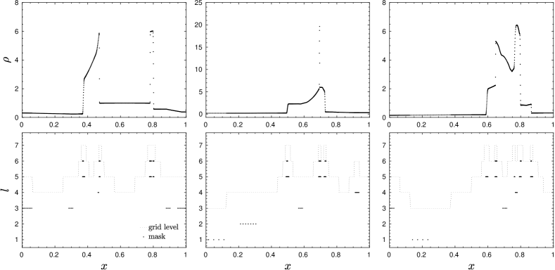
Figure 3: The HAMR solution for the two interacting blast waves problem is shown for density, along with the mesh refinement levels and MR mask (two levels per block), in top and bottom rows, respectively. The evolution is shown before the shocks collide ($t=0.016$; left column), at the time of the collision ($t=0.028$; middle column), and at the final time ($t=0.038$; right column). The MR tolerance in this model is $\varepsilon=1\times 10^{-2}$ and the safety factor is $\kappa=1\times 10^{-1}$ . Note the sparse structure in the MR mask, indicating that the solver adaptive approach can be used to increase efficiency.

the density profile (top row), as well as the mesh structure and associated MR mask (bottom row), is shown at early time ($t=0.016$ s; left column panels) when the two blast waves are fully developed, at the time of their collision ($t=0.028$ s; middle column panels), and at the final time ($t=0.038$ s; right column panels). At the end of simulation the flow structure is refined to the finest level across the interaction region, $x\in\left[0.6,0.8\right]$, bounded by the left contact discontinuity and right-moving transmitted shock. At the adopted level of MR tolerance, the mesh resolves most of the perturbed sections of the flow to the finest level of resolution.

4.2 Hawley-Zabusky problem

In the Hawley-Zabusky (HZ) problem [49], a planar shock wave obliquely strikes a material interface. In the "fast-slow" case of the HZ problem considered here, the shock is initially positioned in the low-density (high sound speed) material. As the time progresses, the shock gradually passes through the interface and refracts. This interaction results in the deposition of vorticity (driven by the baroclinic term), and in consequence material mixing, at the interface.

In our setup, the mesh is initially comprised of six blocks (consisting of $16\times 16$ cells each) in the streamwise direction, and we allow $L=6$ levels of refinement. The MR tolerance is set to $\varepsilon=1\times 10^{-2}$, and we apply the solver adaptive scheme to the fluxes only, with a safety factor of $\kappa=1\times 10^{-2}$. The results corresponding to this choice of parameters are shown in fig. 4.

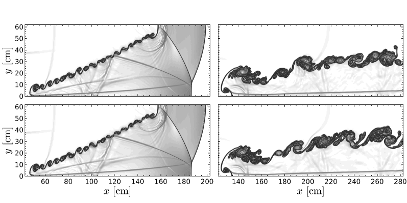
Figure 4: The morphology of the flow in the Hawley-Zabusky problem is shown with numerical schlieren density images for the baseline AMR solution (top row) and HAMR solution with $\kappa=1\times 10^{-2}$ (bottom row). The panels in the left column show the morphology shortly after the shock passed through the interface ($t\approx 180\ $\mathrm{s}$$), while the structure of the interface at the final simulation time is shown in the right column. Note that the structure of the HAMR solution closely matches that of the baseline solution at early times. There are however discernible differences in the small scale structure of the mixed region at the final time. See text for details.

The numerical schlieren density plot obtained with the baseline AMR scheme are shown in the top row, and those obtained with the HAMR scheme are shown in the bottom row at early (left column) and late times (right column) in the figure. As the shock passes through the interface and refracts, vorticity is deposited along the interface (left column panels in fig. 4) resulting in extensive mixing at later times (right column panels in the figure). The conspicuous differences in the morphology of the flow at those late times is a consequence of strong sensitivity to perturbations, in this case introduced by the interpolation of fluxes in the HAMR solution.

4.3 Two-dimensional cellular detonation

The cellular detonation problem [50] is concerned with the growth and evolution of multidimensional instability of the detonation front. We consider this problem as an essential example of the integrated multi-physics applications, with hydrodynamics now combined with a realistic EoS and a set of strongly coupled source terms. A relatively simple one-dimensional profile of the detonation wave is substantially altered if non-radial perturbations are introduced in multidimensional realizations of the problem. In this case, the energy delivered behind various parts of the initially planar detonation front will differ, resulting in nonuniform propagation speed of neighboring segments of the front. Depending on the specific problem conditions, the perturbations organize into a set of separate regions that take the form of cell-like structures.

Our setup for this problem matches that of [50], with the exception of the nuclear network (we use a $7$ isotope network) and a twice narrower computational domain. The domain is covered with 20 blocks in the $x$-direction and one block in the $y$-direction, with the blocks each consisting of $16\times 16$ cells. The maximum number of mesh levels allowed is $L=7$, resulting in an effective model resolution of $1.25\times 10^{-2}\ $\mathrm{cm}$$. This mesh refinement configuration is equivalent to approximately $160$ cells per burning length scale, ensuring that the problem dynamics are well resolved. The refinement variables are density, pressure, and temperature, and the chosen MR tolerance of $\varepsilon=6\times 10^{-1}$ is sufficient to resolve the detonation front to the finest level of mesh resolution.

In fig. 5

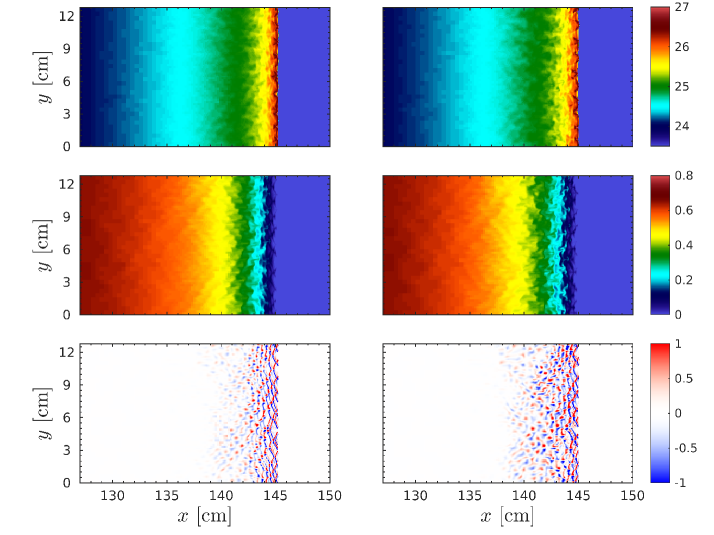
Figure 5: The morphology of the flow in quasi-steady state in the cellular detonation problem for the baseline AMR solution (left column panels) and the HAMR solution with $\kappa=1\times 10^{-1}$ (right column panels). The individual rows of panels show nuclear energy generation rate (top row panels, log scale), silicon abundance (middle row panels), and the $z$-component of vorticity (bottom row panels). The vorticity is shown in units of $10^{9}\ \mathrm{s}^{-1}$. See text for details.

we show select components of the baseline AMR solution (left column panels) and the corresponding HAMR solution (right column panels) obtained with $\kappa=1\times 10^{-1}$ when the system is in quasi-steady state. In both solutions, the triple points can be seen as the local maxima in energy generation rate located along the leading shock front (top row panels in fig. 5). This energy release drives transverse waves which interact with the incident shock, resulting in a complex and inhomogeneous distribution of silicon (second row panels) in the post-detonation region. This process of compositional homogenization can be understood by examining the vorticity field (bottom row panels), which indicates the presence of strong rotational motions, and thus mixing. We note that the two solutions are qualitatively similar, however more diffusive structures are observed in the HAMR solution for the given safety factor. We defer a more detailed comparison of baseline and HAMR solutions for a range of safety factors to section 5.1.

4.4 Reactive turbulence

For the second integrated multi-physics application of the proposed method we select a reactive turbulence problem. Although this application shares several similarities with the cellular detonation problem introduced earlier, here the complex flow and action of source terms are no longer restricted to a narrow region of the problem domain. Furthermore, unlike in the case of detonation studies, turbulence is genuinely multi-dimensional in nature. Also, even though the current study is limited to two spatial dimensions, all of the algorithmic components are examined in the same way as they would be in the three-dimensional case.

The adopted reactive turbulence simulation setup closely matches that of [51], with the mesh being uniformly resolved with $1024$ cells per dimension. Our model differs from that of Brooker et al. in that turbulence is spectrally driven with the energy injected at a rate of $7\times 10^{14}\ \text{ergs}\ \text{s}^{-1}$, and the model is evolved toward quasi-steady state until $t\approx 125\text{ms}$. The models used in the analysis are evolved for about one turnover time on the integral scale ($\approx 40\ \text{ms}$) after the quasi-steady state is reached.

Figure 6

Figure 6: The vorticity field and divergence of velocity in the two-dimensional turbulence model are shown with flooded contours at $t=125\ \text{ms}$ (the beginning of quasi-steady state) and $t=165\ \text{ms}$ (about one turnover time on the integral scale into the quasi-steady state) in the left and right panel, respectively. The solution in the left panel was obtained using the reference scheme, and provided initial conditions for the adaptive solution obtained with $\tilde{\varepsilon}=10^{-3}$, which is shown in the right panel at the later time. The adaptive solution displays qualitatively similar structures as the reference solution, with two counter-rotating vortices dominating the flow on the scale of the computational domain. The narrow, extended structures correspond to the velocity divergence smaller than $-800\ \text{s}^{-1}$, associated with shocklets. Note that this particular realization of the model does not include the effects of nuclear burning.

shows the vorticity field and the velocity divergence in the quasi-steady state at the initial time for the reference model (left panel), and for the adaptive model at the final simulation time (right panel). We choose not to show the solutions at the same time because they do not significantly differ at the final time. Overall the adaptive solution displays similar flow structures to that of the reference solution, with the large scale flow dominated by counter-rotating vortices and numerous shocklets present. We note that in the quasi-steady state the average solution properties are expected to remain the same, which makes qualitative comparison of those two select models meaningful.

5 Discussion

The introduction of the solver adaptive approach affects the solution accuracy and code performance to a varying degree depending on the problem at hand. These two factors are not independent of one another. For example, more frequent replacement of direct calculations with multiresolution-based interpolation, which offers computational savings, is enabled as the multiresolution threshold increases and solution accuracy is accordingly lowered (in general). In this section we discuss various aspects of this relation as well as other factors affecting computational performance of the new scheme.

5.1 Assessment of HAMR solution accuracy

Interaction of two blast waves

To evaluate the impact of the solver adaptive procedure on the numerical solution, we first discuss the results obtained for the one-dimensional interacting blast waves problem (cf. section 4.1). We perform a set of simulations with the MR solver adaptive safety factor $\kappa$ being varied systematically from $10^{-4}$ to $10^{-1}$. Figure 7

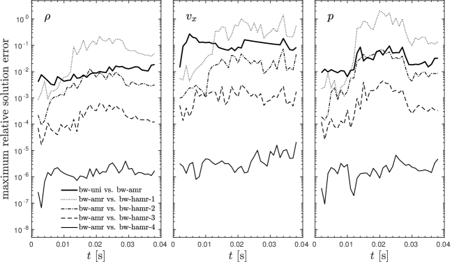
Figure 7: Maximum relative solution error for the interacting blast waves problem. The error at each time is calculated by normalizing the $L_{\infty}$ error norm by the maximum value of the corresponding variable obtained in the uniform mesh solution. The thick solid line shows the error evolution of the AMR solution with respect to the uniform mesh solution. The evolution of the errors obtained with the HAMR scheme with respect to the AMR solution are plotted with thin lines of differing styles as identified in the figure legend. The results are shown for density, velocity, and pressure for select values of the safety factor $\kappa$. The safety factor is changing by a factor of $10$ between the HAMR models.

shows the evolution of the normalized $L_{\infty}$ norm of the differences between the reference and adaptive numerical solutions. It is clear that the accuracy of the HAMR solutions (shown with the family of thin lines of differing styles in fig. 7), as compared with the AMR solution, scale approximately with the safety factor. For example, the error in density (left panel in fig. 7) in the model bw-hamr-1, which corresponds to $\kappa=1\times 10^{-1}$, reaches a value of about $0.2$, while for the model bw-hamr-4, which corresponds to $\kappa=1\times 10^{-4}$, the error never exceeds a value of $1\times 10^{-5}$.

Although the errors in velocity and pressure (middle and right panels in fig. 7, respectively) slightly exceed the density error, the overall scaling with the safety factor appears to hold. This behavior is consistent with the MR analysis provided by [12]. We find these results encouraging because despite the intrusive character of the solver-adaptive approach and highly nonlinear character of the problem, the solution trajectories do not show any inconsistent departures from the reference solution.

One can also quantify the error in the AMR solution by using the uniform mesh as the reference solution. This error, shown with the thick solid line in fig. 7, remains within the expected ranges (recall that the tolerance for mesh adaptation is $\varepsilon=1\times 10^{-2}$) for each of the variables throughout the simulation. The error in the HAMR models with $\kappa=1\times 10^{-4}$ through $\kappa=1\times 10^{-2}$ remain smaller than this, implying that the solver adaptive procedure is not increasing the overall solution error for these values of the safety factor.

Hawley-Zabusky problem

From the perspective of error control, the regions of interest in the HZ problem may appear to be limited to the salient solution features, in particular the shocks and vortices. However, the background flow is in fact extremely rich in this case (we refer the interested reader to [52] for a more detailed description of those flow structures).

Figure 8

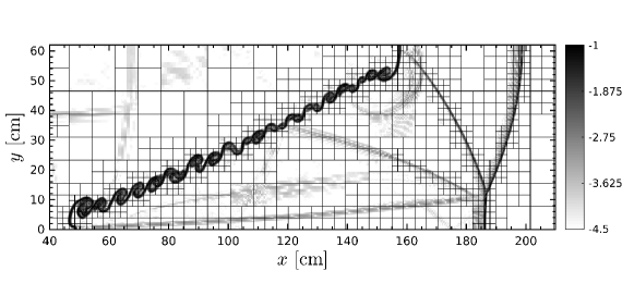
Figure 8: The log of MR detail coefficients on the finest level of each the local MR hierarchy on each AMR block is plotted at time $t\approx 180$\mathrm{s}$$. At the selected MR tolerance of $\varepsilon=1\times 10^{-2}$, the algorithm allocates blocks at the finest AMR level ($L=6$) in two main regions: along the material interface where vorticity is large, and along the passing shock waves, where pressure gradients are large. Near the important solution features there are regions where the mesh is relatively fine (due to the block-based AMR format) but the MR detail coefficients are relatively small, inviting the use of the solver adaptive scheme.

shows the field of MR detail coefficients at $t\approx 180$\mathrm{s}$$, with the AMR block outlines overlaid. When compared with the numerical schlieren image at the same time (see fig. 4), it is evident that the MR detail coefficients closely track the prominent solution features. The coefficients associated with the leading shock, reflected shock, and Mach stem reach their maximal values in excess of $0.1$. These high values force refinement to the finest available AMR level. Meanwhile the weaker acoustic waves reverberating behind the shocks and across the interface result in significantly smaller values of detail coefficients, necessitating less mesh refinement. These values are below the specified MR tolerance, and with the adopted safety factor in this particular model of $\kappa=1\times 10^{-2}$, the corresponding parts of the flow are subject to the solver adaptive scheme.

One of the key quantities characterizing the HZ problem is the vorticity, which is the result of the baroclinic source term driven by the interaction of density and pressure gradients. One can expect that the amount of vorticity produced will sensitively depend on the accuracy of the numerical scheme, and in particular on its ability to describe solution gradients. Likewise the amount of vorticity produced will depend on the prescribed MR tolerance. Also the integrated vorticity better characterizes the overall performance of the solver than, for example, the structure of the interface. This is because the growth of instability across the interface in this problem is limited only by numerical diffusion and thus does not converge under mesh refinement.

Figure 9

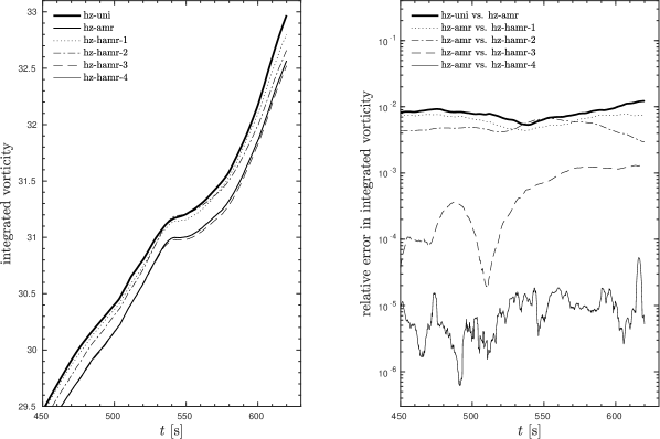
Figure 9: The time evolution of integrated vorticity and its relative error in the Hawley-Zabusky problem at late times. The integrated vorticity evolution is shown in the left panel for the reference uniform mesh solution (thick solid line), AMR solution (medium solid line), and a set of HAMR models (family of thin lines of differing styles). The time evolution of the relative error in integrated vorticity is shown in the right panel during the same time window for each HAMR solution. See text for details.

shows the evolution of integrated vorticity and its relative error for our set of HZ models, where the safety factor varies between $1\times 10^{-4}$ and $1\times 10^{-1}$. The vorticity during the late time discussed here gradually increases, with a temporary plateau around $t\approx 540\ $\mathrm{s}$$ due to a vortex pair merger. The amount of vorticity produced in the AMR model, hz-amr, which serves as the baseline model for the HAMR solutions, is smaller in comparison to the uniform mesh reference model, hz-uni, by nearly $1\%$, but closely follows the general trend. The HAMR model with the least restrictive safety factor of $\kappa=1\times 10^{-1}$, hz-hamr-1, shows the largest deviation away from the baseline hz-amr model, but again the overall trend in the vorticity evolution is preserved. As the solver adaptive tolerance is tightened, the vorticity in the consecutive hz-hamr models converge to the baseline hz-amr model.

Two-dimensional cellular detonation

In the cellular detonation problem the goal is to preserve the cellular structure of the detonation and accurately capture the nuclear energy generation rate, composition of the combustion products, and also the production of vorticity, which is responsible for mixing in the reaction zone behind the front. The last element is also of importance for incomplete burning taking place in the tail of the reaction zone. We note that depending on the adopted threshold this extended reaction zone is only partially resolved.

In our study, the safety factors range from $1\times 10^{-3}$ to $1\times 10^{-1}$. Figure 10

Figure 10: Errors in lateral averages of energy generation rate, abundance of silicon, and vorticity in the reaction zone for the cellular detonation problem. The solver adaptive approach is applied to the hydrodynamic fluxes, Helmholtz EoS, and the reactive source term, and the safety factor ranges from $\kappa=10^{-3}$ to $\kappa=10^{-1}$.

shows the $L_{\infty}$ error norm in lateral averages of energy generation rate, silicon abundance, and vorticity at the final simulated time. The respective errors are normalized by the $L_{\infty}$ value obtained in the reference AMR model, cd-ref. It is evident from the left panel of fig. 10 that in the case of the cd-hamr-1 model, the maximal error in energy generation rate is approximately equal to the adopted AMR tolerance of $\varepsilon=1\times 10^{-1}$. This implies that the error in this quantity due to the solver adaptive scheme is not dominating the overall solution error.

The middle panel of fig. 10 shows the distribution of silicon, which is the main product of burning in this problem. The error in this quantity is well controlled in all HAMR models. The error in vorticity, shown in the right panel of fig. 10, is the greatest in the model cd-hamr-1, and exceeds that of the AMR tolerance ($\approx 0.8$ vs. $0.6$). However, lowering the safety factor produces much more satisfactory results in both energy generation rate and vorticity. One item to note is the crossing of error curves in vorticity between the models cd-hamr-2 and cd-hamr-3 in the trailing edge of the reaction zone ($\approx 140$ cm). We speculate that one possible reason for that behavior is the highly unsteady character of the solution, which naturally results in unsteady behavior of errors.

The primary source of solution errors in this problem is the leading shock front, the associated reaction zone, and the detonation cells. These features are clearly captured by the MR decomposition, as illustrated by the distribution of detail coefficients in fig. 11.

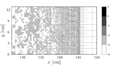
Figure 11: Mesh structure and MR detail coefficients for the cellular detonation problem in the cd-ref model. The mesh structure is indicated by the outlines of the individual mesh blocks (each block contains $16\times 16$ cells). The detail coefficients are shown in the log scale with flooded contours. Note that upstream of the detonation front the values of the detail coefficients are zero.

Also, it should be noted that the interpolation of fluxes, EoS outputs, and source terms is relatively active inside the reaction zone in the cd-hamr-1 model compared to models with a smaller value of the safety factor. This is not unexpected given that this region contains pockets of relative smoothness between the detonation cells and also in the detonation cell interiors. An example is the intercell region near $(x,y)\approx(145,9)$ and the detonation cell interior near $(x,y)\approx(145,11)$. In effect, in the coarse model cd-hamr-1, the highly nonlinear part of the solution dominated by burning is fed with a significant perturbation that is due to MR interpolation. However as soon as the energy generation rate is added to the set of mask indicator variables, the solver adaptive mask covers the entire reaction zone, and consequently no interpolation is performed. Overall the distribution of detail coefficients correctly reflects on the smoothness of the flow downstream of the detonation front, resulting in a gradual decrease in mesh resolution.

Reactive turbulence

One of the fundamental statistics used to characterize isotropic, homogeneous turbulence is the kinetic energy spectrum. The theory of turbulence predicts a universal scaling law in the intertial range, with kinetic energy of velocity fluctuations (KE) to scale as $k^{-3}$ in two-dimensional situations, as predicted by Kraichnan [53]. It is reproducing this behavior in numerical experiments that provides elemental confidence in simulation outcomes. Figure 12

Figure 12: The turbulent kinetic energy spectra in the reactive turbulence problem. The energy spectrum in the reference non-adaptive solution as a function of wavenumber, $k$, is shown in the left panel along with the Kraichnan $k^{-3}$ scaling law, indicated with a straight line segment. The relative error for each of the solver adaptive models is shown in the right panel. The solver adaptive tolerances range from $\tilde{\varepsilon}=10^{-3.5}$ to $\tilde{\varepsilon}=10^{-3.0}$. Note that the error values are consistent with the chosen tolerance of the adaptive scheme.

shows the kinetic energy spectra (left panel) and respective errors (right panel) in our set of numerical experiments. The errors in the solver adaptive solutions were calculated with respect to the reference, non-adaptive model. The overall shape of the kinetic energy spectra matches closely that of the theoretical $k^{-3}$ scaling relation. As in the previous test cases, the errors in the KE spectra obtained with the solver adaptive solutions appear to vary in a way consistent with the changes in the solver adaptive tolerance, $\tilde{\varepsilon}$. However, we were unable to obtain satisfactory solutions with tolerances greater than $\tilde{\varepsilon}=1\times 10^{-3}$. In such heavily interpolated models the solution structure displayed numerical artifacts in the form of undershoots and overshoots in the solution components. Furthermore, a relatively small tightening of the tolerance resulted in a disproportionately large improvement in the solution quality. We speculate that this behavior might be attributed to thermodynamically inconsistent MR interpolation of the EoS. The thermodynamic consistency of the Helmholtz EoS was shown by Timmes & Swesty [5] to be of crucial importance for obtaining physically relevant solutions.

In the previously discussed problems our focus was not necessarily focused on the primitive solution components but rather on the solution functionals, as they are of main interest from the application point of view. Some examples here are the vorticity in the Hawley-Zabusky problem, and the production of silicon in the cellular detonation problem. Likewise here our focus is on the ignition time, $\tau_{\mathrm{ig}}$. This quantity describes the potential of the physical system to develop deflagrations and detonations, which qualitatively change the system evolution. Therefore it is particularly important for the numerical scheme to correctly describe a part of the solution containing the shortest ignition times.

One way of characterizing various populations of ignition times is to construct a histogram of mass as a function of ignition time. Such a histogram is shown for our set of reactive turbulence models in the left panel of fig. 13.

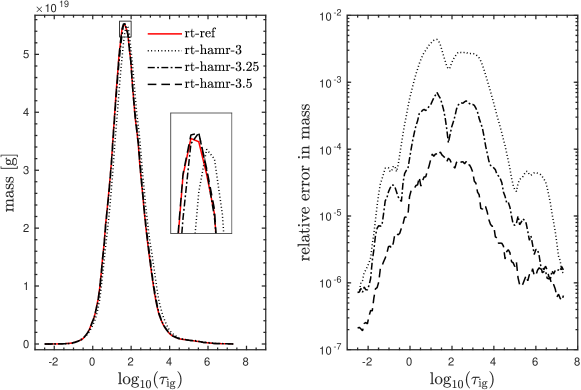
Figure 13: The mass distribution as a function of ignition times in the reactive turbulence problem is shown for a set of adaptive solutions (left panel). The solver adaptive tolerances range from $\tilde{\varepsilon}=10^{-3.5}$ to $\tilde{\varepsilon}=10^{-3.0}$, with $\tilde{\varepsilon}=0$ corresponding to the reference case. The inset shows in detail the mass distributions near their peak values. The relative error in mass distribution is shown in the right panel. The line styles used to plot the relative error correspond to the legend in the left panel. Note that the mass distributions as well as their respective errors show systematic deviations with relatively less mass at short ignition times as the error tolerance becomes less stringent.

Although it is encouraging to see the overall shape of the distributions obtained from adaptive models closely matching the reference distribution, a closer inspection of histogram data reveals some systematic differences. The inset plot in the left panel in the figure shows a closeup view of the region near the peaks of the distributions. We observe the increasing amount of mass at longer ignition times as the tolerance $\tilde{\varepsilon}$ is progressively more relaxed. This is confirmed by the examination of differences of mass distributions obtained from solver adaptive models with that of the reference model (right panel in fig. 13). The observed behavior can be understood as the result of greater numerical dissipation in more heavily interpolated models, which results in the decrease of amplitudes of turbulent fluctuations and therefore the decrease of the number of fluid parcels with short ignition times. From the application point of view, the consequence of the added dissipation is that the deflagration ignition process or the process of transition to detonation may not be truthfully described in heavily interpolated models. This is consistent with our earlier conclusion that in this application in which there is an extremely strong dependence of the source term on temperature, the numerical convergence is problematic and demands good control over the error.

5.2 Computational efficiency

To analyze the savings offered by the solver adaptive scheme in terms of computational cost, Harten [12] introduced the efficiency factor, which compares the number of cells used to obtain the non-adaptive model to the number of cells used to obtain the corresponding MR model. We adapt Harten’s definition to be compatible with block-structured AMR format as follows. The number of cells in the mesh at timestep $n$ is $|\bm{\mathcal{B}}^{n}|N_{\mathcal{L}}$, where $|\bm{\mathcal{B}}^{n}|$ is the total number of leaf blocks, and the total number of cells in the adaptive mask over the collection of blocks is $\sum_{b=1}^{|\bm{\mathcal{B}}^{n}|}N_{1}+|\bm{\mathcal{M}}_{b}^{n}|$, where $|\bm{\mathcal{M}}_{b}^{n}|$ is the number of cells included in the local mask of block $b$. With these terms introduced, we define the efficiency factor to be the ratio of the total number of cells used in the simulation to the total number of adaptive evaluations,

$$\eta=\frac{\sum_{n=1}^{n_{\Delta t}}|\bm{\mathcal{B}}^{n}|N_{\mathcal{L}}}{\sum_{n=1}^{n_{\Delta t}}\left(\sum_{b=1}^{|\bm{\mathcal{B}}^{n}|}N_{1}+|\bm{\mathcal{M}}_{b}^{n}|\right)},$$ (21)

where $n_{\Delta t}$ is the total number of timesteps. Note that the so-defined efficiency factor provides the maximal estimate of possible savings and typically provides an upper bound for the reduction in time-to-solution of computer simulations.

To enable a more direct comparison between solver components, we define the efficiency factors with respect to each module as $\eta_{\mathrm{hydro}}$, $\eta_{\mathrm{eos}}$, and $\eta_{\mathrm{burn}}$. These will differ from one another due to the unique attributes of each module. For example, the reactive source term is not activated unless the density and temperature are sufficiently high.

To measure improvements in execution times, we adopt the speedup factor of Bihari [16],

$$\zeta=\frac{\mathrm{runtime\ per\ call\ without\ solver\ adaptivity}}{\mathrm{runtime\ per\ call\ with\ solver\ adaptivity}}.$$ (22)

The runtime is measured on a per-call basis. This is because the trajectory of the solution obtained with the solver adaptive scheme may differ from the trajectory of the solution obtained without solver adaptivity. In consequence the AMR refinement pattern may differ as well, requiring a different number of calls to the individual solver components.

As in the case of the efficiency factor, we calculate speedup factors for the individual solver components, labeling the factors as $\zeta_{\mathrm{hydro}}$, $\zeta_{\mathrm{eos}}$, and $\zeta_{\mathrm{burn}}$. We reiterate that these speedup factors will in general be smaller than the corresponding efficiency factors defined earlier.

Interaction of two blast waves

For the problem of two interacting blast waves, the HAMR scheme achieves a significant reduction in the number of fluxes evaluated, while maintaining solution accuracy compared with the baseline bw-amr model (see section 5.1). Table 1

Table 1: Computational efficiency data for the interacting blast waves problem. The efficiency factor, $\eta_{\mathrm{hydro}}$, and the reduction in the number of fluxes compared with the baseline model bw-amr are shown as a function of the safety factor, $\kappa$.

$\kappa$	$\eta_{\mathrm{hydro}}$	fraction of fluxes
$10^{-1}$	1.46	0.68
$10^{-2}$	1.29	0.78
$10^{-3}$	1.20	0.83
$10^{-4}$	1.18	0.85

provides computational efficiency data, which includes the efficiency factor and information about the reduction in the number of fluxes computed compared to the model bw-amr. The collected data indicates that for models that we deem acceptable from the solution accuracy point of view, one may expect efficiency factors between about $1.2$ to $1.3$. Relative to the baseline AMR model, bw-amr, the fraction of evaluated fluxes for these models is about $0.8$. We conclude that for this problem dominated by a relatively few strong, localized discontinuities always resolved to the finest AMR level, the scheme achieves a performance improvement of roughly $20\%$.

Hawley-Zabusky problem

In the HZ problem the mesh filling factor is significantly greater than in the interacting blast waves problem due to the mixing of fluid along the interface. For this reason one may expect less performance gain from the HAMR approach. The data in table 2

Table 2: Efficiency factor, $\eta_{\mathrm{hydro}}$, and speedup factors, $\zeta_{\mathrm{intrfc}}$, $\zeta_{\mathrm{states}}$, $\zeta_{\mathrm{rieman}}$, for the Hawley-Zabusky problem with $L=6$ and $L=7$ levels of refinement, and an AMR tolerance of $\varepsilon=0.01$, respectively. A range of safety factors are tested, with the baseline AMR model corresponding to $\kappa=0$.

$L$	$\kappa$	$\eta_{\mathrm{hydro}}$	$\zeta_{\mathrm{intrfc}}$	$\zeta_{\mathrm{states}}$	$\zeta_{\mathrm{rieman}}$	$\zeta_{\mathrm{hydro}}$	$t_{\mathrm{wall}}($\mathrm{h}$)$
$6$	$10^{-1}$	1.37	1.14	1.22	1.26	1.20	3.58
$6$	$10^{-2}$	1.15	1.08	1.10	1.12	1.10	3.71
$6$	$10^{-3}$	1.06	1.02	1.03	1.04	1.03	3.74
$6$	$10^{-4}$	1.04	1.02	1.03	1.03	1.03	3.74
$6$	$0$	–	–	–	–	–	3.76
$7$	$10^{-1}$	1.34	1.14	1.19	1.22	1.18	19.41
$7$	$10^{-2}$	1.16	1.07	1.08	1.09	1.08	21.02
$7$	$10^{-3}$	1.06	1.01	1.02	1.03	1.02	21.11
$7$	$10^{-4}$	1.03	1.01	1.02	1.02	1.02	21.36
$7$	$0$	–	–	–	–	–	21.46

confirms this expectation. In particular, the obtained efficiency factors are around $1.1$ for models with a still acceptable quality ($\kappa$ between $1\times 10^{-3}$ and $1\times 10^{-2}$). Also, the speedup factors for the individual components of the hydro solver are typically less than $1.1$ for that range of models. Furthermore the performance gains are less for intrfc than for states and rieman modules because of the poorer data locality for the (interface) reconstruction part of the PPM algorithm. Finally, we speculate that the improvement in simulation wallclock time is probably hindered by the exacerbated load imbalance due to a difference in computational cost between blocks where some fraction of fluxes were interpolated, and those blocks where no such interpolation was used. The set of results obtained with mesh resolution increased by a factor of $2$ ($L=7$ in the table) displays similar trends, although the gains are somewhat smaller perhaps due to the increased complexity of the small scale structure.

Cellular detonation problem

The efficiency data for the cellular detonation problem is shown in table 3.

Table 3: Computational efficiency data for the cellular detonation problem. The table shows the efficiency factors, $\eta_{\mathrm{hydro}}$, $\eta_{\mathrm{eos}}$, and $\eta_{\mathrm{burn}}$, and speedup factors, $\zeta_{hydro}$, $\zeta_{eos}$, and $\zeta_{burn}$ for solutions obtained with with $L=7$ and $L=8$ levels of refinement. The chosen AMR tolerance for these models is $\varepsilon=0.6$. Results for several runs obtained with a range of safety factors are presented with the baseline AMR model corresponding to $\kappa=0$.

$L$	$\kappa$	$\eta_{\mathrm{hydro}}$	$\eta_{\mathrm{eos}}$	$\eta_{\mathrm{burn}}$	$\zeta_{\mathrm{hydro}}$	$\zeta_{\mathrm{eos}}$	$\zeta_{\mathrm{burn}}$	$t_{\mathrm{wall}}($\mathrm{h}$)$
$7$	$10^{-1}$	1.47	2.14	1.55	1.15	1.25	1.18	2.57
$7$	$10^{-2}$	1.31	1.58	1.05	1.12	1.14	1.02	2.60
$7$	$10^{-3}$	1.30	1.51	1.00	1.11	1.11	0.99	2.62
$7$	$0$	–	–	–	–	–	–	2.64
$8$	$10^{-1}$	1.55	2.12	1.57	1.15	1.23	1.19	5.55
$8$	$10^{-2}$	1.29	1.55	1.08	1.11	1.12	1.02	5.89
$8$	$10^{-3}$	1.27	1.46	1.01	1.11	1.10	0.99	5.95
$8$	$0$	–	–	–	–	–	–	5.99

The data now include two additional physics describing the thermodynamics via a complex EoS, and the reactive source term for nuclear energy generation. The hydrodynamics module shows somewhat better performance compared to the two pure hydrodynamics problems due to the heavily interpolated ambient medium upstream of the detonation front. The same level of performance oberserved for the hydrodynamics is also observed in the EoS module. This kind of superficial performance improvement does not apply to burning however, because the code omits calculation of the nuclear burning source term if the temperature is too low, as is the case in the cold fuel region upstream of the shock. Furthermore, the MR analysis does not allow any interpolation inside the reaction zone for values of $\kappa$ below $1\times 10^{-2}$. For this reason, we observe no speedup ($\zeta_{\mathrm{burn}}=0.99$) for the model with $\kappa=1\times 10^{-3}$. Similar trends are observed in the higher resolution ($L=8$) model.

Reactive turbulence problem

Unlike in the previous problems discussed, the turbulence problem is characterized by the presence of substantial flow structure occupying the entire domain, and on all scales. This is reflected by the relatively narrow range of solver adaptive tolerances that we considered for this problem (cf. section 4.4), where we found that for coarse tolerances the solution appeared polluted by numerical artifacts, while there was no interpolation performed for tolerances of about an order of magnitude tighter. In consequence, the solver adaptive approach was enabled only in relatively small parts of the solution. We found that for the model rt-hamr-3 ($\tilde{\varepsilon}=1\times 10^{-3}$), the speedup factors were at most a few percent for the reactive source term, while there were no noticeable gains for the hydro or EoS solver components. For the remaining models, no speedup was observed for any of the solver components. We conclude that for turbulence models, the strong coupling between the thermodynamically sensitive equation of state and nonlinear hydrodynamics appears to make the problem effectively intractable from the point of view of solver-adaptivity.

5.3 Overall performance considerations

We considered a set of applications ranging from a shock-dominated one-dimensional flow problem to complex multi-dimensional, multi-physics situations using the proposed HAMR scheme. In each of these applications, the domain is occupied by a small number of discontinuous flow features (e.g. shocks) against a rich background (e.g. reflected acoustic waves). Furthermore, the prominent flow features interact with each other frequently and create new, complicated structures. With respect to these situations the discussion of the overall performance of the HAMR scheme naturally turns to two main points: the efficiency of the MR-driven AMR mesh, and the deviation of the solver adaptive solution trajectory from the reference solution trajectory.

We find that the filling factor at the block level is what primarily determines the gains offered by adding solver adaptivity to the MR-driven AMR approach. This is in contrast to the classic AMR computations in which the computational efficiency is determined by the overall mesh filling factor (cf. section 1). In situations where the block filling factor is high, the solver adaptive scheme typically offers little reduction in computational complexity with essentially no savings in computational time. This issue is evident in the problem of reactive turbulence, for which we did not observe a significant gain from solver adaptivity. However, one can anticipate that such gains would be offered in the case of inhomogeneous turbulence, where the solution contains, for example, a flame front (discontinuous structure) that separates fuel from burning products. In particular, studies of deflagrations in the distributed burning regime appear especially suitable for the HAMR approaches.

In general we expect modeling of turbulence with the solver adaptive approach to be challenging. This is because, as we observed in an extended set of reactive turbulence simulations, the accumulation of interpolation error caused progressive deviation of the solver adaptive solutions away from the reference solution. That is we observed significant differences between the solutions at late times. Therefore, the solver adaptive approach may not be suitable for problems expected to produce new phenomena after a transient period of evolution. We note that much the same accumulation of error is expected to occur in pure AMR simulations as well, for example in studies of homogeneous turbulence where the mesh blocks are continuously created and destroyed depending on the local smoothness of the solution.

We note that our set of application examples are more typical of basic physics or discovery science studies rather than engineering problems. The former class of problems, for example, are frequently characterized by very high Reynolds numbers and thus prone to produce increasing amounts of structure in the solution as mesh resolution increases. A representative example from our application studies is the HZ problem, in which the small scale structure in the mixed region is limited only by the numerical dissipation of the solver. Had the HZ problem included sub-grid scale viscous dissipation models typically used in engineering applications, the amount of small scale structure would be limited, with the results converging upon adequate mesh refinement. In such an engineering model, one could expect that the HAMR scheme would be increasingly more efficient, as the solution would be progressively more interpolated due to an increase in the amount of solution regions with sufficient smoothness.

Also, there might be situations when the physics problem is demanding not necessarily in terms of space and time, but in terms of the physics model description. Some classes of these types of problems are radiation transport models with complex opacities, and combustion models with large reaction networks. In the latter case, one does not expect gains from HAMR approach inside the reaction zone (cf. section 4.3), but this changes in the downstream region where multiple reaction products are advected. In that region the source term is essentially inactive, but the hydrodynamic evolution is potentially several times more expensive to compute because of the increased number of fluxes. Therefore one expects that these classes of problems may be better suited for the HAMR-type approaches.

5.4 Aspects of implementation

The solver adaptive approach operates on outputs provided by the solver. From the implementation point of view, this requires communicating information between the solver and the interpolation operator. For example, the source term and equation of state interpolation both operate directly on the cell average values, and therefore share common MR data structures and interpolation routines. On the other hand, in the case of the directionally split hydrodynamic solver, different MR data structures and interpolation routines are needed, especially when the values being operated on are associated with cell interfaces (requiring pointwise interpolation). In general other types of solvers (such as particle-based) may require dedicated implementations of those MR components.

Provided that the MR components are readily available, the main implementation challenge is to appropriately interface them with the existing solvers. This is potentially quite challenging because some solvers do not operate only on local data, but require additional information from the neighborhood of the current point. One example are reconstruction-evolution schemes which may use long data stencils. In such cases, more substantial reduction of the computational of the solver can be obtained by integrating the MR components at a lower level of the solver. This means that one may be required to modify the internal structures, such as individual loops, of those solver modules.

In our experience with the PPM implementation available in the flash code, particular components of the algorithm had to be converted from vector-like to scalar-like computations. Generally, the latter strategy is less efficient on modern computer architectures, but as we demonstrated the replacement of direct calculations with interpolation still proves beneficial in terms of computational cost. Alternative approaches may rely on repackaging the input data such that solver kernel operates on a subset of data. We found this approach to produce a computationally inefficient code due to a substantial amount of data copy operations. The version of the PPM solver accompanying this paper relies on the former fine-grained approach which restricts calculations at the loop level.

6 Summary

Harten originally developed his seminal solver adaptive multiresolution approach for hydrodynamics problems on uniform meshes. The novelty of the proposed HAMR method is the extension of Harten’s scheme to MR-driven AMR discretizations and multi-physics applications. The new scheme addresses the deficiency of block-structured AMR that occurs when only a fraction of mesh cells in an AMR block is used to resolve the structure that triggered mesh refinement. In those situations the remaining mesh cells inside the block describe the smooth part of the flow, which makes them amenable to the solver adaptive approach.

We evaluated the performance of the HAMR-based code using several test problems. Our findings indicate that the performance gains offered by the new approach mainly depend on the AMR block mesh filling factor, which expresses the ratio of the number of cells marked for refinement to the overall number of cells in the block. This factor depends on the application type, and for a specific application type varies within the computational domain. The computational gains are the highest for the cases in which the solution exhibits highly localized features; smaller gains are expected in the case of spatially extended solution structures. This characteristic is not surprising and is consistent with the performance characteristic of AMR schemes.

The results of the numerical experiments performed indicate that the error due to the solver adaptive component can be controlled adequately by using a separate solver adaptive tolerance. Thus, the computational gains offered by the solver adaptive approach are shown to be achieved while solution accuracy, as prespecified by the user, remains under control.

The current work opens a number of avenues for future research. For example, we expect HAMR to offer increased gains with the increased problem complexity, and therefore it would be of interest to further study the dependence of the efficiency on the application type. Also, as most high fidelity simulations are performed on large, parallel computer systems, the load balancing characteristics of AMR solvers equipped with the solver adaptive component are expected to change and may require optimization. The public version of our HAMR implementation can be used as a starting point for these kinds of studies.

References

-
[1]
J. H. Chen,
Petascale
direct numerical simulation of turbulent combustion-fundamental insights
towards predictive models, Proceedings of the Combustion Institute 33 (1)
(2011) 99 – 123.
doi:https://doi.org/10.1016/j.proci.2010.09.012.
URL http://www.sciencedirect.com/science/article/pii/S1540748910003962 -
[2]
D. Fenn, T. Plewa, Detonability of
white dwarf plasma: turbulence models at low densities, Monthly Notices of
the Royal Astronomical Society 468 (2) (2017) 1361–1372.
arXiv:https://academic.oup.com/mnras/article-pdf/468/2/1361/11126950/stx524.pdf,
doi:10.1093/mnras/stx524.
URL https://doi.org/10.1093/mnras/stx524 - [3] E. S. Oran, J. P. Boris, Numerical Simulation of Reactive Flow, 2nd Edition, Cambridge University Press, 2000. doi:10.1017/CBO9780511574474.
-
[4]
Y. B. Zel’dovich, V. B. Librovich, G. M. Makhviladze, G. I. Sivashinskil,
On the onset of detonation in a
nonuniformly heated gas, Journal of Applied Mechanics and Technical Physics
11 (2) (1970) 264–270.
doi:10.1007/BF00908106.
URL https://doi.org/10.1007/BF00908106 -
[5]
F. X. Timmes, F. D. Swesty, The
accuracy, consistency, and speed of an electron-positron equation of state
based on table interpolation of the helmholtz free energy, The Astrophysical
Journal Supplement Series 126 (2) (2000) 501–516.
doi:10.1086/313304.
URL https://doi.org/10.1086%2F313304 -
[6]
M. J. Berger, J. Oliger,
Adaptive
mesh refinement for hyperbolic partial differential equations, Journal of
Computational Physics 53 (3) (1984) 484 – 512.
doi:https://doi.org/10.1016/0021-9991(84)90073-1.
URL http://www.sciencedirect.com/science/article/pii/0021999184900731 -
[7]
J. J. Quirk,
A
parallel adaptive grid algorithm for computational shock hydrodynamics,
Applied Numerical Mathematics 20 (4) (1996) 427 – 453, adaptive mesh
refinement methods for CFD applications.
doi:https://doi.org/10.1016/0168-9274(95)00105-0.
URL http://www.sciencedirect.com/science/article/pii/0168927495001050 -
[8]
R. Löhner,
An
adaptive finite element scheme for transient problems in cfd, Computer
Methods in Applied Mechanics and Engineering 61 (3) (1987) 323 – 338.
doi:https://doi.org/10.1016/0045-7825(87)90098-3.
URL http://www.sciencedirect.com/science/article/pii/0045782587900983 -
[9]
S. Li,
Comparison
of refinement criteria for structured adaptive mesh refinement, Journal of
Computational and Applied Mathematics 233 (12) (2010) 3139 – 3147, finite
Element Methods in Engineering and Science (FEMTEC 2009).
doi:https://doi.org/10.1016/j.cam.2009.08.104.
URL http://www.sciencedirect.com/science/article/pii/S037704270900586X -
[10]
K. Schneider, O. V. Vasilyev,
Wavelet methods in
computational fluid dynamics, Annual Review of Fluid Mechanics 42 (1) (2010)
473–503.
arXiv:https://doi.org/10.1146/annurev-fluid-121108-145637, doi:10.1146/annurev-fluid-121108-145637.
URL https://doi.org/10.1146/annurev-fluid-121108-145637 -
[11]
A. Harten, Multiresolution
representation of data: A general framework, SIAM Journal on Numerical
Analysis 33 (3) (1996) 1205–1256.
URL http://www.jstor.org/stable/2158503 -
[12]
A. Harten,
Adaptive
multiresolution schemes for shock computations, Journal of Computational
Physics 115 (2) (1994) 319 – 338.
doi:https://doi.org/10.1006/jcph.1994.1199.
URL http://www.sciencedirect.com/science/article/pii/S0021999184711995 -
[13]
A. Harten,
Multiresolution
algorithms for the numerical solution of hyperbolic conservation laws,
Communications on Pure and Applied Mathematics 48 (12) (1995) 1305–1342.
arXiv:https://onlinelibrary.wiley.com/doi/pdf/10.1002/cpa.3160481201,
doi:10.1002/cpa.3160481201.
URL https://onlinelibrary.wiley.com/doi/abs/10.1002/cpa.3160481201 -
[14]
B. L. Bihari,
Multiresolution
schemes for conservation laws with viscosity, Journal of Computational
Physics 123 (1) (1996) 207 – 225.
doi:https://doi.org/10.1006/jcph.1996.0017.
URL http://www.sciencedirect.com/science/article/pii/S0021999196900170 -
[15]
B. L. Bihari, A. Harten,
Multiresolution schemes for
the numerical solution of 2-d conservation laws i, SIAM Journal on
Scientific Computing 18 (2) (1997) 315–354.
arXiv:https://doi.org/10.1137/S1064827594278848, doi:10.1137/S1064827594278848.
URL https://doi.org/10.1137/S1064827594278848 -
[16]
B. L. Bihari, D. Schwendeman,
Multiresolution
schemes for the reactive euler equations, Journal of Computational Physics
154 (1) (1999) 197 – 230.
doi:https://doi.org/10.1006/jcph.1999.6312.
URL http://www.sciencedirect.com/science/article/pii/S002199919996312X -
[17]
G. Chiavassa, R. Donat, Point
value multiscale algorithms for 2d compressible flows, SIAM J. Sci. Comput.
23 (3) (2001) 805–823.
doi:10.1137/S1064827599363988.
URL https://doi.org/10.1137/S1064827599363988 - [18] B. Gottschlich-Müller, S. Müller, Adaptive finite volume schemes for conservation laws based on local multiresolution techniques, in: M. Fey, R. Jeltsch (Eds.), Hyperbolic Problems: Theory, Numerics, Applications, Birkhäuser Basel, Basel, 1999, pp. 385–394.
-
[19]
M. K. Kaibara, S. M. Gomes,
A Fully Adaptive
Multiresolution Scheme for Shock Computations, Springer US, Boston, MA,
2001, pp. 497–503.
doi:10.1007/978-1-4615-0663-8_49.
URL https://doi.org/10.1007/978-1-4615-0663-8_49 - [20] A. Cohen, S. M. Kaber, S. Müller, M. Postel, Fully adaptive multiresolution finite volume schemes for conservation laws, Math. Comput. 72 (2003) 183–225.
-
[21]
O. Roussel, K. Schneider, A. Tsigulin, H. Bockhorn,
A
conservative fully adaptive multiresolution algorithm for parabolic pdes,
Journal of Computational Physics 188 (2) (2003) 493 – 523.
doi:https://doi.org/10.1016/S0021-9991(03)00189-X.
URL http://www.sciencedirect.com/science/article/pii/S002199910300189X -
[22]
O. Roussel, K. Schneider,
An
adaptive multiresolution method for combustion problems: application to flame
ball-vortex interaction, Computers & Fluids 34 (7) (2005) 817 – 831.
doi:https://doi.org/10.1016/j.compfluid.2004.05.011.
URL http://www.sciencedirect.com/science/article/pii/S0045793004001136 -
[23]
O. Roussel, K. Schneider,
Adaptive
multiresolution computations applied to detonations, Zeitschrift für
Physikalische Chemie 229 (6) (28 Jun. 2015) 931 – 953.
doi:https://doi.org/10.1515/zpch-2014-0574.
URL https://www.degruyter.com/view/journals/zpch/229/6/article-p931.xml -
[24]
M. O. Domingues, S. M. Gomes, O. Roussel, K. Schneider,
An
adaptive multiresolution scheme with local time stepping for evolutionary
pdes, Journal of Computational Physics 227 (8) (2008) 3758 – 3780.
doi:https://doi.org/10.1016/j.jcp.2007.11.046.
URL http://www.sciencedirect.com/science/article/pii/S0021999107005219 - [25] M. O. Domingues, S. M. Gomes, O. Roussel, K. Schneider, Space–time adaptive multiresolution methods for hyperbolic conservation laws: Applications to compressible euler equations, Applied Numerical Mathematics 59 (2009) 2303–2321.
-
[26]
A. Khokhlov,
Fully
threaded tree algorithms for adaptive refinement fluid dynamics simulations,
Journal of Computational Physics 143 (2) (1998) 519 – 543.
doi:https://doi.org/10.1006/jcph.1998.9998.
URL http://www.sciencedirect.com/science/article/pii/S0021999198999983 -
[27]
K. G. Powell, P. L. Roe, T. J. Linde, T. I. Gombosi, D. L. De Zeeuw,
A
solution-adaptive upwind scheme for ideal magnetohydrodynamics, Journal of
Computational Physics 154 (2) (1999) 284 – 309.
doi:https://doi.org/10.1006/jcph.1999.6299.
URL http://www.sciencedirect.com/science/article/pii/S002199919996299X -
[28]
B. T. Gunney, R. W. Anderson,
Advances
in patch-based adaptive mesh refinement scalability, Journal of Parallel and
Distributed Computing 89 (2016) 65 – 84.
doi:https://doi.org/10.1016/j.jpdc.2015.11.005.
URL http://www.sciencedirect.com/science/article/pii/S0743731515002129 - [29] B. Van Straalen, J. Shalf, T. Ligocki, N. Keen, Woo-Sun Yang, Scalability challenges for massively parallel amr applications, in: 2009 IEEE International Symposium on Parallel Distributed Processing, 2009, pp. 1–12. doi:10.1109/IPDPS.2009.5161014.
-
[30]
A. Peplinski, P. F. Fischer, P. Schlatter,
Parallel performance of h-type
adaptive mesh refinement for nek5000, in: Proceedings of the Exascale
Applications and Software Conference 2016, EASC ’16, Association for
Computing Machinery, New York, NY, USA, 2016.
doi:10.1145/2938615.2938620.
URL https://doi.org/10.1145/2938615.2938620 -
[31]
B. Fryxell, K. Olson, P. Ricker, F. X. Timmes, M. Zingale, D. Q. Lamb,
P. MacNeice, R. Rosner, J. W. Truran, H. Tufo,
FLASH: An adaptive mesh
hydrodynamics code for modeling astrophysical thermonuclear flashes, The
Astrophysical Journal Supplement Series 131 (1) (2000) 273–334.
doi:10.1086/317361.
URL https://doi.org/10.1086%2F317361 - [32] R. T. Fisher, L. P. Kadanoff, D. Q. Lamb, A. Dubey, T. Plewa, A. Calder, F. Cattaneo, P. Constantin, I. Foster, M. E. Papka, S. I. Abarzhi, S. M. Asida, P. M. Rich, C. C. Glendenin, K. Antypas, D. J. Sheeler, L. B. Reid, B. Gallagher, S. G. Needham, Terascale turbulence computation using the flash3 application framework on the ibm blue gene/l system, IBM Journal of Research and Development 52 (1.2) (2008) 127–136. doi:10.1147/rd.521.0127.
- [33] C. for Computational Sciences, L. B. N. L. Engineering, Boxlib, Available at https://ccse.lbl.gov/BoxLib.
-
[34]
W. Zhang, A. Almgren, V. Beckner, J. Bell, J. Blaschke, C. Chan, M. Day,
B. Friesen, K. Gott, D. Graves, M. P. Katz, A. Myers, T. Nguyen, A. Nonaka,
M. Rosso, S. Williams, M. Zingale,
Amrex: a framework for
block-structured adaptive mesh refinement, Journal of Open Source Software
4 (37) (2019) 1370.
doi:10.21105/joss.01370.
URL https://doi.org/10.21105/joss.01370 - [35] A. M. Wissink, R. Hornung, S. Kohn, S. Smith, N. Elliott, Large scale parallel structured amr calculations using the samrai framework, ACM/IEEE SC 2001 Conference (SC’01) (2001) 22–22.
- [36] R. Deiterding, Amroc - blockstructured adaptive mesh refinement in object-oriented c++, Available at http://amroc.sourceforge.net.
- [37] M. Adams, et al., Chombo software package for AMR applications - design document.
-
[38]
F. Schornbaum, U. RÃŒde,
Extreme-scale block-structured
adaptive mesh refinement, SIAM Journal on Scientific Computing 40 (3) (2018)
C358–C387.
arXiv:https://doi.org/10.1137/17M1128411, doi:10.1137/17M1128411.
URL https://doi.org/10.1137/17M1128411 -
[39]
L. Han, X. Hu, N. Adams,
Adaptive
multi-resolution method for compressible multi-phase flows with sharp
interface model and pyramid data structure, Journal of Computational Physics
262 (2014) 131 – 152.
doi:https://doi.org/10.1016/j.jcp.2013.12.061.
URL http://www.sciencedirect.com/science/article/pii/S0021999114000230 - [40] M. Sroka, T. Engels, P. Krah, S. Mutzel, K. Schneider, J. Reiss, An open and parallel multiresolution framework using block-based adaptive grids, in: R. King (Ed.), Active Flow and Combustion Control 2018, Springer International Publishing, Cham, 2019, pp. 305–319.
-
[41]
R. Deiterding, M. O. Domingues, K. Schneider,
Multiresolution
analysis as a criterion for effective dynamic mesh adaptation - a case study
for euler equations in the samr framework amroc, Computers & Fluids 205
(2020) 104583.
doi:https://doi.org/10.1016/j.compfluid.2020.104583.
URL http://www.sciencedirect.com/science/article/pii/S0045793020301559 -
[42]
S. MacNamara, G. Strang,
Operator Splitting,
Springer International Publishing, Cham, 2016, pp. 95–114.
doi:10.1007/978-3-319-41589-5_3.
URL https://doi.org/10.1007/978-3-319-41589-5_3 - [43] R. Courant, K. Friedrichs, H. Lewy, On the partial difference equations of mathematical physics, IBM Journal of Research and Development 11 (2) (1967) 215–234.
-
[44]
S. K. Godunov, I. Bohachevsky,
Finite difference
method for numerical computation of discontinuous solutions of the equations
of fluid dynamics, Matematičeskij sbornik 47(89) (3) (1959)
271–306.
URL https://hal.archives-ouvertes.fr/hal-01620642 -
[45]
N. Hovhannisyan, S. Müller, On
the stability of fully adaptive multiscale schemes for conservation laws
using approximate flux and source reconstruction strategies, IMA Journal of
Numerical Analysis 30 (4) (2009) 1256–1295.
arXiv:https://academic.oup.com/imajna/article-pdf/30/4/1256/2066941/drp010.pdf,
doi:10.1093/imanum/drp010.
URL https://doi.org/10.1093/imanum/drp010 -
[46]
P. Colella, P. R. Woodward,
The
piecewise parabolic method (ppm) for gas-dynamical simulations, Journal of
Computational Physics 54 (1) (1984) 174 – 201.
doi:https://doi.org/10.1016/0021-9991(84)90143-8.
URL http://www.sciencedirect.com/science/article/pii/0021999184901438 -
[47]
F. X. Timmes, R. D. Hoffman, S. E. Woosley,
An inexpensive nuclear energy
generation network for stellar hydrodynamics, The Astrophysical Journal
Supplement Series 129 (1) (2000) 377–398.
doi:10.1086/313407.
URL https://doi.org/10.1086%2F313407 -
[48]
P. Woodward, P. Colella,
The
numerical simulation of two-dimensional fluid flow with strong shocks,
Journal of Computational Physics 54 (1) (1984) 115 – 173.
doi:https://doi.org/10.1016/0021-9991(84)90142-6.
URL http://www.sciencedirect.com/science/article/pii/0021999184901426 -
[49]
J. F. Hawley, N. J. Zabusky,
Vortex paradigm
for shock-accelerated density-stratified interfaces, Phys. Rev. Lett. 63
(1989) 1241–1244.
doi:10.1103/PhysRevLett.63.1241.
URL https://link.aps.org/doi/10.1103/PhysRevLett.63.1241 -
[50]
F. X. Timmes, M. Zingale, K. Olson, B. Fryxell, P. Ricker, A. C. Calder, L. J.
Dursi, H. Tufo, P. MacNeice, J. W. Truran, R. Rosner,
On the cellular structure of carbon
detonations, The Astrophysical Journal 543 (2) (2000) 938–954.
doi:10.1086/317135.
URL https://doi.org/10.1086%2F317135 - [51] E. Brooker, T. Plewa, D. Fenn, SN Ia DDT Explosions Powered by the Zeldovich Reactivity Gradient MechanismarXiv:2008.05010.
-
[52]
N. J. Zabusky, Vortex
paradigm for accelerated inhomogeneous flows: Visiometrics for the
rayleigh-taylor and richtmyer-meshkov environments, Annual Review of Fluid
Mechanics 31 (1) (1999) 495–536.
arXiv:https://doi.org/10.1146/annurev.fluid.31.1.495, doi:10.1146/annurev.fluid.31.1.495.
URL https://doi.org/10.1146/annurev.fluid.31.1.495 - [53] R. H. Kraichnan, Inertial Ranges in Two-Dimensional Turbulence, Physics of Fluids 10 (7) (1967) 1417–1423. doi:10.1063/1.1762301.