Efficient high-harmonic generation in graphene with two-color laser field at orthogonal polarization

Abstract

High-order frequency mixing in graphene using a two-color radiation field consisting of the fundamental and the second harmonic fields of an ultrashort linearly polarized laser pulse is studied. It is shown that the harmonics originated from the interband transitions are efficiently generated in the case of the orthogonally polarized two-color field. In this case, the generated high-harmonics are stronger than those obtained in the parallel polarization case by more than two orders of magnitude. This is in sharp contrast with the atomic and semiconductor systems, where parallel polarization case is more preferable. The physical origin of this enhancement is also deduced from the three-step semi-classical electron-hole collision model, extended to graphene with pseudo-relativistic energy dispersion. In particular, we discuss the influence of the many particle Coulomb interaction on the HHG process within dynamical Hartree-Fock approximation. Our analysis shows that in all cases we have an overall enhancement of the HHG signal compared with the free-charged carrier model due to the electron-hole attractive interaction.

I Introduction

Significant experimental and theoretical efforts have recently been invested in the generation of high-order harmonics (HHG) of a laser field interacting with the condensed phase of the matter. The generation of harmonics has recently been reported in solid-state materials with crystalline symmetry [1, 2, 3, 4, 5, 6, 7, 8, 9, 10, 11, 12, 13, 14, 15, 16], in amorphous solids [17], and in liquids [18], which ensures that the condensed phase of the matter has the potential of becoming a compact and efficient attosecond light source of the next-generation due to the high density of the emitters, compared with a gaseous medium. HHG gives access to a frequency range that is difficult to achieve in other ways [19], and provides a frequency-domain view of the electron dynamics in quantum systems [20]. The complete characterization of the radiated harmonic spectrum, phase, and polarization will allow to recover the underlying quasiparticle dynamics in solids. In particular, using HHG one can reconstruct the crystal potential and electrons density with a spatial resolution of about 10 picometres [21], which can be used for the direct investigation of the electronic and topological properties of the materials. From the spectra of HHG in crystals one can observe the dynamical Bloch oscillations [5], Mott [22], and Peierls [23] transitions, retrieve the band-structure [24, 25] or the band topology [26].

The HHG in atomic gases has been intensively investigated since the 90s of the last century [27] and now with the advent of controlled few-cycle light waves is the basis of the attosecond science [28, 29]. In view of the vast theoretical and experimental methods developed for atomic HHG, it is of interest to analyze whether methods that were developed for enhancing HHG in the gas phase are also applicable to HHG in solid state nanostructures. Among the existing nanostructures, the graphene due to its more pronounced properties allows to use it as a more effective nonlinear optical material and has triggered many studies devoted to nonperturbative HHG [30, 31, 32, 33, 34, 35, 36, 37, 38, 39, 40, 41, 42, 43, 44, 45]. Specifically, diverse polarization and ellipticity dependence effects in the total HHG spectrum [42, 43, 44, 45] are revealed in a monolayer graphene where interaction with the pump wave drives charged carriers far away from the Dirac cones. The latter opens up wide opportunities for increasing the HHG yield in graphene by choosing the parameters of the driving wave.

An efficient option for increasing the HHG yield in atomic systems is the use of multicolor driving pulses. High-order wave mixing processes with multi-color laser fields have gained enormous interest due to the additional degrees of freedom, such as relative polarizations, intensities, phases, and wavelengths of involved pump waves. In atomic systems, it has been shown that adding an additional second or third harmonic field can enhance the HHG in the plateau region by several orders of magnitude [46, 47, 48]. The HHG with different compositions of the driving laser pulses was addressed also for solid targets and nanostructures considering two distinct regimes: First, if the driving field consists of the fundamental wave and its harmonics [4, 24, 49, 50, 51, 52, 53, 54, 55], and second, if one of the involved wave frequencies significantly higher than the other one [2, 56, 57, 58, 59, 60, 61, 62]. Two-color high-order wave mixing research reported so far has mainly been performed for gapped systems. For 2D semimetals, two-color high-order wave mixing was considered in Ref. [61] in case when one of the frequencies significantly higher than the other one. In Ref. [55] it was considered valley-selective HHG in pristine graphene by using a combination of the two counter-rotating circularly polarized fields. For solid targets with an energy gap exposed to two- or three-color laser pulses [49, 52, 54] of parallel polarizations the enhancement of HHG has been shown in an analogy with the atomic HHG [46], where the HHG in the orthogonally polarized two-color field is suppressed. The latter is intuitively clear in terms of a simple quasiclassical three-step model [28, 29]. As far as the polarization of resultant field is no longer linear, the ionized electron will, in general, never return to the parent ion. However, for gapless systems, as will be shown in the current paper, this conclusion does not hold, and the opposite applies: the HHG yield will be increased considerably at the orthogonally polarized two-color driving wave fields.

In this paper the high-order frequency mixing in graphene using a two-color radiation field that consisted of the fundamental and the second harmonic (SH) fields of an ultrashort linearly polarized laser pulse is studied. It is shown that the harmonics originated from the interband transitions are efficiently generated in the case of the orthogonally polarized two-color laser field. This is in sharp contrast with the atomic [46] and semiconductor cases [54] where the parallel polarization case is more preferable.

We consider a rather general model, including many-particle Coulomb interaction, since the Coulomb interaction is known to be generally stronger in low-dimensional structures. The importance of Coulomb interaction for ultrafast many-particle kinetics in graphene has been theoretically and experimentally verified [63, 64, 65]. The significance of many-body Coulomb interaction at the high harmonic generation process in graphene has been shown in Ref. [40]. The latter study was conducted near the Dirac points and the open question of interest remains: to develop the theory of HHG with many-body Coulomb interaction beyond the Dirac cone approximation that is applicable to the full Brillouin zone (BZ) [64]. As a first step, the combined carrier-carrier and carrier-phonon scatterings are taken into account phenomenologically with relaxation rate in femtosecond time-scale [63].

The paper is organized as follows. In Sec. II the evolutionary equation for the single-particle density matrix is presented. The electron-electron Coulomb interaction is taken into account within the dynamical Hartree-Fock (HF) approximation [66, 65] beyond the Dirac cone approximation and applicable to the full Brillouin zone of a hexagonal tight-binding nanostructure. In Sec. III, we consider HHG spectra and present the main results. Finally, conclusions are given in Sec. IV.

II The evolutionary equation for the single-particle density matrix

We consider the interaction of a strong two-color laser field $\mathbf{E}(t)$ with graphene. The waves propagate in a perpendicular direction to the monolayer plane ($XY$) of graphene with the electric field strength:

$$\mathbf{E}\left(t\right)=f_{1}\left(t\right)E_{01}\hat{\mathbf{e}}_{1}\cos\left(\omega t\right)+f_{2}\left(t\right)E_{02}\hat{\mathbf{e}}_{2}\cos\left(2\omega t\right),$$ (1)

where $E_{01}$ and $E_{02}$ are the amplitudes of the laser pulses, $\omega$ is the fundamental frequency, $\hat{\mathbf{e}}_{1}$ and $\hat{\mathbf{e}}_{2}$ are the unit polarization vectors. The envelopes of the two wave-pulses are described by the sin-squared functions

$$f_{1,2}(t)=\left\{\begin{array}[]{cc}\sin^{2}\left(\pi t/\tau_{1,2}\right),&0\leq t\leq\tau_{1,2},\\ 0,&t<0,t>\tau_{1,2},\end{array}\right.$$ (2)

where $\tau_{1}$ and $\tau_{2}$ characterize the pulse duration. The carrier-envelope phases for both wave-pulses are set to zero.

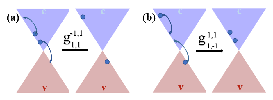
Figure 1: Schematic representation of the Coulomb-induced MA processes near the Dirac cone for destruction (a) and multiplication (b) of carriers in one specific band at the expense of another band.

The dynamics of the system is governed by the total Hamiltonian:

$$\hat{H}=\hat{H}_{\mathrm{free}}+\hat{H}_{\mathrm{C}}+\hat{H}_{\mathrm{int}},$$ (3)

where

$$\hat{H}_{\mathrm{\ free}}=\sum_{\lambda,\mathbf{k}}\mathcal{E}_{\lambda}\left(\mathbf{k}\right)\hat{e}_{\lambda\mathbf{k}}^{\dagger}\hat{e}_{\lambda\mathbf{k}}$$ (4)

is the free particle Hamiltonian, with $\hat{e}_{\lambda\mathbf{k}}$ ($\hat{e}_{\lambda\mathbf{k}}^{\dagger}$) the annihilation (creation) operators for an electron with the momentum $\mathbf{k}$ and band index $\lambda=\pm 1\widehat{=}c,v$ (for conduction ($\lambda=1$) and valence ($\lambda=-1$) bands). In Eq. (4) $\mathcal{E}_{c}\left(\mathbf{k}\right)$ and $\mathcal{E}_{v}\left(\mathbf{k}\right)$ are the corresponding band energy dispersions. The specific expressions for the single-particle Hamiltonian and other derived quantities are given in the Appendix. In HF approximation, we reduce the Coulomb interaction Hamiltonian $\hat{H}_{\mathrm{C}}$ into the mean-field Hamiltonian:

$$\hat{H}_{\mathrm{C}}=-\ \sum\limits_{\alpha\beta\gamma\delta}\sum\limits_{\mathbf{k}\neq\mathbf{k}^{\prime}}g_{\gamma,\beta}^{\alpha,\delta}\left(\mathbf{k,k}^{\prime}\right)V_{2D}(\mathbf{k}^{\prime}-\mathbf{k})\rho_{\gamma\delta}\left(\mathbf{k}^{\prime},t\right)\hat{e}_{\alpha\mathbf{k}}^{\dagger}\hat{e}_{\beta\mathbf{k}}.$$ (5)

where $V_{2D}\left(\mathbf{k}\right)$ is the Fourier transform of the electron-electron interaction potential and the form factor reads:

$$g_{\gamma,\beta}^{\alpha,\delta}\left(\mathbf{k,k}^{\prime}\right)=\frac{1}{4}\left(1+\alpha\gamma\delta\beta+\left(\delta\beta+\alpha\gamma\right)f_{c}\left(\mathbf{k,k}^{\prime}\right)\right.$$

$$\left.+i\left(\delta\beta-\alpha\gamma\right)f_{s}\left(\mathbf{k,k}^{\prime}\right)\right).$$ (6)

In Eq. (5) $\rho_{\gamma\delta}\left(\mathbf{k}^{\prime},t\right)=\left\langle\widehat{e}_{\delta\mathbf{k}^{\prime}}^{\dagger}\widehat{e}_{\gamma\mathbf{k}^{\prime}}\right\rangle$ is the single particle density matrix, and the functions

$$f_{c}\left(\mathbf{k,k}^{\prime}\right) = \mathrm{Re}\left\{\frac{f^{\ast}\left(\mathbf{k}\right)f\left(\mathbf{k}^{\prime}\right)}{\left|f\left(\mathbf{k}\right)\right|\left|f\left(\mathbf{k}^{\prime}\right)\right|}\right\},$$

$$f_{s}\left(\mathbf{k,k}^{\prime}\right) = \mathrm{Im}\left\{\frac{f^{\ast}\left(\mathbf{k}\right)f\left(\mathbf{k}^{\prime}\right)}{\left|f\left(\mathbf{k}\right)\right|\left|f\left(\mathbf{k}^{\prime}\right)\right|}\right\}$$

are defined via the structure function $f\left(\mathbf{k}\right)$ (32). The terms in Eq. (5) proportional to $f_{s}\left(\mathbf{k,k}^{\prime}\right)$ are nonzero when $\delta\beta=-\alpha\gamma$, and describe Meitner-Auger processes [67, 68, 69]. A Meitner-Auger (MA) process is a Coulomb-induced interaction for which the number of carriers in the bands are not conserved individually, cp. Fig. 1. In graphene, due to a vanishing bandgap, these processes cannot be neglected, in contrast to conventional semiconductors when a large bandgap suppresses the MA effect by the demand of energy conservation. The two major MA processes for electrons, corresponding to the Coulomb matrix elements $g_{1,1}^{-1,1}\left(\mathbf{k,k}^{\prime}\right)$ and $g_{1,-1}^{1,1}\left(\mathbf{k,k}^{\prime}\right)$ for destruction (a) and multiplication (b) of carriers in one specific band at the expense of another band are displayed in Fig. 1. For holes, similar processes occur.

The last term in Eq. (3)

$$\hat{H}_{\mathrm{int}}=ie\mathbf{E}(t)\sum\limits_{\alpha\beta}\sum\limits_{\mathbf{kk}^{\prime}}\int\left(\partial_{\mathbf{k}}e^{i\left(\mathbf{k}^{\prime}-\mathbf{k}\right)\mathbf{r}}\right)d\mathbf{r}\langle\alpha\mathbf{k}||\beta\mathbf{k}^{\prime}\rangle\ \hat{e}_{\alpha\mathbf{k}}^{\dagger}\hat{e}_{\beta\mathbf{k}^{\prime}}$$ (7)

is the the light-matter interaction Hamiltonian in the length gauge, $e$ is the elementary charge, and

$$\langle\alpha\mathbf{k}||\beta\mathbf{k}^{\prime}\rangle=\frac{1}{2}\left(f_{c}\left(\mathbf{k,k}^{\prime}\right)+if_{s}\left(\mathbf{k,k}^{\prime}\right)+\alpha\beta\right).$$

Now, from the Heisenberg equation $i\hbar\partial_{t}\hat{e}_{\alpha\mathbf{k}}^{\dagger}\hat{e}_{\beta\mathbf{k}}=\left[\hat{e}_{\alpha\mathbf{k}}^{\dagger}\hat{e}_{\beta\mathbf{k}},\hat{H}\right]$ one can obtain the closed set of evolutionary equations for a density matrix $\rho_{\beta,\alpha}(k,t)=\left\langle\hat{e}_{\alpha\mathbf{k}}^{\dagger}\hat{e}_{\beta\mathbf{k}}\right\rangle$. The diagonal elements represent particle distribution functions for conduction $\mathcal{N}_{c}(\mathbf{k},t)=\rho_{1,1}(\mathbf{k},t)$ and valence $\mathcal{N}_{v}(\mathbf{k},t)=\rho_{-1,-1}(\mathbf{k},t)$ bands, and the non-diagonal element is the interband polarization $\mathcal{P}(\mathbf{k},t)=\rho_{1,-1}(\mathbf{k},t)$. On the HF level for an undoped system in equilibrium, the initial conditions $\mathcal{P}(\mathbf{k},0)=0$, $\mathcal{N}_{c}^{0}(\mathbf{k})=0$, and $\mathcal{N}_{v}^{0}(\mathbf{k})=1$ are assumed, neglecting thermal occupations or doping. Since $\mathcal{N}_{v}(\mathbf{k},t)=1-$ $\mathcal{N}_{c}(\mathbf{k},t)$, the equation for $\mathcal{N}_{v}(\mathbf{k},t)$ is superficial. Thus, the graphene interaction with a strong laser field is modeled as:

$$\partial_{t}\mathcal{N}_{c}(\mathbf{k},t)-\hbar^{-1}e\mathbf{E}\left(t\right)\partial_{\mathbf{k}}\mathcal{N}_{c}(\mathbf{k},t)=$$

$$-2\mathrm{Im}\left\{\left[\hbar^{-1}\mathbf{E}\left(t\right)\mathbf{D}_{\mathrm{tr}}\left(\mathbf{k}\right)+\Omega_{c}\left(\mathbf{k},t;\mathcal{P},\mathcal{N}_{c}\right)\right]\mathcal{P}^{\ast}(\mathbf{k},t)\right\},$$ (8)

$$\partial_{t}\mathcal{P}(\mathbf{k},t)-\hbar^{-1}e\mathbf{E}\left(t\right)\partial_{\mathbf{k}}\mathcal{P}(\mathbf{k},t)=$$

$$-i\hbar^{-1}\left[\mathcal{E}_{c}\left(\mathbf{k}\right)-\mathcal{E}_{v}\left(\mathbf{k}\right)-\Xi_{c}(\mathbf{k},t;\mathcal{P},\mathcal{N}_{c})-i\hbar\Gamma\right]\mathcal{P}(\mathbf{k},t)$$

$$+i\left[\hbar^{-1}\mathbf{E}\left(t\right)\mathbf{D}_{\mathrm{tr}}\left(\mathbf{k}\right)+\Omega_{c}\left(\mathbf{k},t;\mathcal{P},\mathcal{N}_{c}\right)\right]\left[1-2\mathcal{N}_{c}(\mathbf{k},t)\right],$$ (9)

where $\mathbf{D}_{\mathrm{tr}}\left(\mathbf{k}\right)=-e\langle c,\mathbf{k}|i\partial_{\mathbf{k}}|v,\mathbf{k}\rangle$ is the transition dipole moment, $\Gamma$ is the phenomenological relaxation rate. The many-body Coulomb interaction renormalizes the light-matter coupling via the internal dipole field of all generated electron-hole excitations:

$$\Omega_{c}\left(\mathbf{k},t;\mathcal{P},\mathcal{N}_{c}\right)=\frac{\hbar^{-1}}{\left(2\pi\right)^{2}}\int_{BZ}d\mathbf{k}^{\prime}V_{2D}\left(\mathbf{k-k}^{\prime}\right)$$

$$\times\left\{\mathcal{P}^{\prime}\left(\mathbf{k}^{\prime},t\right)+if_{c}\left(\mathbf{k,k}^{\prime}\right)\mathcal{P}^{\prime\prime}\left(\mathbf{k}^{\prime},t\right)-if_{s}\left(\mathbf{k,k}^{\prime}\right)\mathcal{N}_{c}\left(\mathbf{k}^{\prime},t\right)\right\},$$ (10)

as well as the transition energies:

$$\Xi_{c}(\mathbf{k},t;\mathcal{P},\mathcal{N}_{c})=\frac{2}{\left(2\pi\right)^{2}}\int_{BZ}d\mathbf{k}^{\prime}V_{2D}\left(\mathbf{k-k}^{\prime}\right)$$

$$\times\left\{f_{c}\left(\mathbf{k,k}^{\prime}\right)\mathcal{N}_{c}\left(\mathbf{k}^{\prime},t\right)+f_{s}\left(\mathbf{k,k}^{\prime}\right)\mathcal{P}^{\prime\prime}\left(\mathbf{k}^{\prime},t\right)\right\}.$$ (11)

From Eqs. (8) and (9) one can recover semiconductor Bloch equations for an ideal 2D semiconductor [70] taking $f_{c}\left(\mathbf{k,k}^{\prime}\right)=1$ and $f_{s}\left(\mathbf{k,k}^{\prime}\right)=0$. The Coulomb contribution (11) in Eq. (9) describes the repulsive electron-electron interaction and leads to a renormalization of the single-particle energy $\mathcal{E}_{c,v}\left(\mathbf{k}\right)$. Note that the Coulomb-induced self-energy has been absorbed into the definition of the single-particle energy and will not be written explicitly hereafter. The Coulomb contribution Eq. (10) leads to a renormalization of the Rabi frequency and accounts for electron-hole attraction. Already in linear spectroscopy this term is responsible for the formation of excitons in semiconductors. In graphene, it gives rise to so-called saddle-point exciton [71, 72] near the van Hove singularity of graphene BZ.

The optical excitation induces a surface current that can be calculated by the following formula:

$$\mathbf{j}\left(t\right)=-2e\sum\limits_{\mathbf{k,}\lambda,\lambda^{\prime}}\rho_{\lambda,\lambda^{\prime}}(\mathbf{k},t)\langle\lambda^{\prime},\mathbf{k}|\widehat{\mathbf{v}}\left(\mathbf{k}\right)|\lambda,\mathbf{k}\rangle.$$ (12)

Here $\widehat{\mathbf{v}}\left(\mathbf{k}\right)$ is the velocity operator, and factor two takes into account spin degeneracy. Note that since we are integrating over the entire Brillouin zone, only the spin-degeneracy has been taken into account.

For the numerical solution of Eqs. (8) and (9), we can make a change of variables and transform the partial differential equations into ordinary ones. The new variables are $t$ and $\mathbf{k}_{0}=\mathbf{k}-\mathbf{k}_{E}$, where $\mathbf{k}_{E}\left(t\right)=-e/\hbar\int_{0}^{t}\mathbf{E}\left(t^{\prime}\right)dt^{\prime}$ is the classical momentum given by the wave field. The latter can be expressed by the vector potential of the laser field: $\mathbf{A}_{L}\mathbf{=-}c^{-1}\int_{0}^{t}\mathbf{E}\left(t^{\prime}\right)dt^{\prime}$ ($c$ is the light speed in vacuum). Throughout this paper, for compactness of equations we will use the notation $\mathbf{A=}e\mathbf{A}_{L}/c\hbar$ for the vector potential. In the new variables Eqs. (8) and (9) read:

$$\partial_{t}\mathcal{N}_{c}(\mathbf{k}_{0},t)=-2\mathrm{Im}\left\{\left[\hbar^{-1}\mathbf{E}\left(t\right)\mathbf{D}_{\mathrm{tr}}\left(\mathbf{k}_{0}+\mathbf{A}\right)\right.\right.$$

$$\left.\left.+\Omega_{c}\left(\mathbf{k}_{0}+\mathbf{A},t;\mathcal{P},\mathcal{N}_{c}\right)\right]\mathcal{P}^{\ast}(\mathbf{k}_{0},t)\right\},$$ (13)

$$\partial_{t}\mathcal{P}(\mathbf{k}_{0},t)=-i\hbar^{-1}\left[\mathcal{E}_{eh}\left(\mathbf{k}_{0}+\mathbf{A}\right)-i\hbar\Gamma\right]\mathcal{P}(\mathbf{k}_{0},t)$$

$$+i\left[\hbar^{-1}\mathbf{E}\left(t\right)\mathbf{D}_{\mathrm{tr}}\left(\mathbf{k}_{0}+\mathbf{A}\right)+\Omega_{c}\left(\mathbf{k}_{0}+\mathbf{A},t;\mathcal{P},\mathcal{N}_{c}\right)\right]$$

$$\times\left[1-2\mathcal{N}_{c}(\mathbf{k}_{0},t)\right],$$ (14)

where $\mathcal{E}_{eh}\left(\mathbf{k}\right)=\mathcal{E}_{c}\left(\mathbf{k}\right)-\mathcal{E}_{v}\left(\mathbf{k}\right)-\Xi_{c}(\mathbf{k},t;\mathcal{P},\mathcal{N}_{c})$ is the electron-hole energy. This set of equations is equivalent to Eqs. (8) and (9), since the gradient term $\mathbf{E}\left(t\right)\partial_{\mathbf{k}}$ and the time-dependent crystal momentum $\mathbf{k}_{0}+\mathbf{A}\left(t\right)$ in Eqs. (13) and (14) describe the same effect. Without Coulomb terms Eqs. (13) and (14) are semiconductor-Bloch equation within the Houston basis [73, 74]. The surface current Eq. ( 12) can be split into the interband and intraband parts as follow:

$$\mathbf{j}_{e}\left(t\right)=-\frac{2e}{(2\pi)^{2}}\int_{\widetilde{BZ}}d\mathbf{k}_{0}\left[\mathbf{v}_{\mathrm{tr}}^{\ast}\left(\mathbf{k}_{0}+\mathbf{A}\right)\mathcal{P}(\mathbf{k}_{0},t)+\mathrm{c.c}\right],$$ (15)

$$\mathbf{j}_{a}\left(t\right)=-\frac{2e}{(2\pi)^{2}}\int_{\widetilde{BZ}}d\mathbf{k}_{0}\left[\mathbf{v}_{c}\left(\mathbf{k}_{0}+\mathbf{A}\right)\mathcal{N}_{c}\left(\mathbf{k}_{0},t\right)+\mathrm{c.c}\right],$$ (16)

where $\mathbf{v}_{\mathrm{tr}}\left(\mathbf{k}\right)=i\left(\mathcal{E}_{c}\left(\mathbf{k}\right)-\mathcal{E}_{v}\left(\mathbf{k}\right)\right)\mathbf{D}_{\mathrm{tr}}\left(\mathbf{k}\right)/e\hbar\$is the transition matrix element for velocity and $\mathbf{v}_{c}\left(\mathbf{k}\right)=\hbar^{-1}\partial\mathcal{E}_{c}\left(\mathbf{k}\right)/\partial\mathbf{k}\$is the mean velocity of the conduction band. In Eqs. (15) and (16) we have taken into account electron-hole symmetry and the BZ is also shifted to $\widetilde{BZ}=BZ-\mathbf{A}$.

The electron-electron interaction potential is modelled by screened Coulomb potential [64]:

$$V_{2D}\left(\mathbf{q}\right)=\frac{2\pi e^{2}}{\epsilon\epsilon_{\mathbf{q}}\left|\mathbf{q}\right|},$$ (17)

which accounts for the substrate-induced screening in the 2D nanostructure ($\epsilon$) and the screening stemming from other valence electrons ($\epsilon_{\mathbf{q}}$). Here, $\epsilon\equiv\left(\epsilon_{1}+\epsilon_{2}\right)/2$, with the dielectric constants of the above $\epsilon_{1}$ and below $\epsilon_{2}$ surrounding media. Assuming a graphene layer on a SiO₂ substrate ($\epsilon_{1}=1$, $\epsilon_{2}=3.9$), we approximate $\epsilon=2.45$. The screening induced by graphene valence electrons is calculated within the Lindhard approximation of the dielectric function $\epsilon_{\mathbf{q}}$, which in a static limit reads: $\triangleq$

$$\epsilon_{\mathbf{q}}=1-\frac{4\pi e^{2}}{\epsilon\left|\mathbf{q}\right|}$$

$$\times\sum_{\lambda,\lambda^{\prime},\mathbf{k}}\digamma_{\lambda,\lambda^{\prime}}\left(\mathbf{k,q}\right)\frac{\mathcal{N}_{\lambda^{\prime}}^{0}\left(\mathbf{k-q}\right)-\mathcal{N}_{\lambda}^{0}\left(\mathbf{k}\right)}{\mathcal{E}_{\lambda^{\prime}}\left(\mathbf{k-q}\right)-\mathcal{E}_{\lambda}\left(\mathbf{k}\right)},$$ (18)

where $\digamma_{\lambda\lambda^{\prime}}\left(\mathbf{k,q}\right)=\frac{1}{2}\left(1+\lambda^{\prime}\lambda f_{c}\left(\mathbf{k,k}-\mathbf{q}\right)\right)$ is the band overlap function.

Figure 2: Particle distribution function $\mathcal{N}_{c}\left(\mathbf{k},t_{f}\right)$ (in arbitrary units) after the interaction for graphene, as a function of scaled dimensionless momentum components ($k_{x}/k_{b}$, $k_{y}/k_{b}$) for different relative polarizations of the fields. The fundamental frequency is $\omega=0.1\ \mathrm{eV}/\hbar$ and the field strength is taken to be $E_{01}=E_{02}=4\ \mathrm{MV/cm}$ (intensity $2.\,13\times 10^{10}\mathrm{W\ cm}^{-2}$).

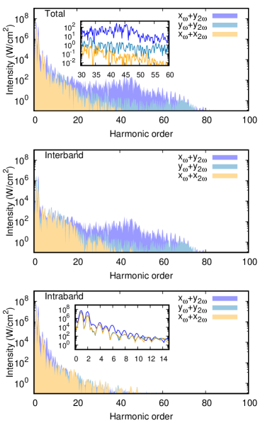
Figure 3: The HHG spectra in logarithmic scale for graphene in the strong-field regime for different relative polarizations of fundamental and SH pump fields. The insets show the middle and the beginning of the spectra. The fundamental frequency is $\omega=0.1\ \mathrm{eV}/\hbar$ and the field strength is taken to be $E_{01}=E_{02}=4\ \mathrm{MV/cm}$.

III Results

In this section we discuss full numerical solution of the quantum HF equations (III.1) and to get more analytical insight, we study which effects can be already observed in a semiclassical approach (III.2).

III.1 Fully Quantum Calculations

We explore the nonlinear response of graphene in a two-color laser field of ultrashort duration. We take a 5-cycle fundamental laser field. The envelopes and amplitudes of fundamental and SH fields are taken to be the same: $E_{0}\equiv E_{01}=E_{02}$ and $\tau\equiv\tau_{1}=\tau_{2}$. The amplitude of fundamental field was varied up to $8\ \mathrm{MV/cm}$ (intensity $8.\,\allowbreak 5\times 10^{10}\ \mathrm{W/cm}^{2}$). Hence, the maximal intensity $1.\,\allowbreak 7\times 10^{11}\ \mathrm{W/cm}^{2}$ impending on graphene is below the damage threshold for monolayer graphene [12, 75, 76]. For all calculations, the relaxation time is taken to be equal to the wave period $\Gamma^{-1}=T=2\pi/\omega$. For the considered frequencies we will have $\Gamma^{-1}=20-40\ \mathrm{fs}$, which is close to the experimental data [63]. The combined laser field possesses $C_{1}$ symmetry [77], hence the allowed harmonic orders are $n\pm 1$, i.e. we have both even and odd harmonics. For sufficiently large 2D sample the generated electric field far from the graphene layer is proportional to the surface current: $\mathbf{E}^{(g)}(t)=-2\pi[\mathbf{j}_{e}(t)+\mathbf{j}_{a}(t)]/c$. The HHG spectral intensity is calculated from the Fourier transform of the generated field.

Figure 4: The HHG spectra for graphene in the strong-field regime for different relative polarizations of fundamental and SH pump fields. (a) The fundamental frequency is $\omega=0.1\ \mathrm{eV}/\hbar$ and the field strength is taken to be $E_{01}=E_{02}=6\ \mathrm{MV/cm}$. (b) The fundamental frequency is $\omega=0.2\ \mathrm{eV}/\hbar$ and the field strength is taken to be $E_{01}=E_{02}=8\ \mathrm{MV/cm}$.

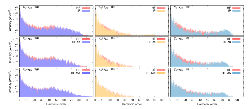
Figure 5: The influence of the Coulomb interaction on the HHG process. The fundamental frequency is $\omega=0.1\ \mathrm{eV}/\hbar$ and the field strength is taken to be $E_{01}=E_{02}=4\ \mathrm{MV/cm}$. (a-c) comparison of $\omega+2\omega$ frequency mixing signals for graphene with independent particles (IP) and with screened Coulomb interaction in the HF level for different relative polarizations of fundamental and SH pump fields. (d-f) comparison of full HF results with HF approximation when only the repulsive part of the electron-electron interaction is switched on. (g-i) comparison of full HF results with HF approximation when MA processes are switched off.

Thus, we have a set of nonlinear integro-differential equations (13) and (14), which have been solved numerically. The time propagation is considered via fourth-order Runge-Kutta method. The numerically demanding parts at each time step are the Coulomb contributions (10) and (11), which are integrated over the full BZ divided to $\sim$10⁵ parts. These terms are calculated using the convolution theorem along with the fast Fourier transform. This procedure decreases computational time by two orders compared with the direct evolution. For integration, we take rhombic BZ, where $\Gamma-K$ line is the x-axis. For the convergence of the results we take $400\times 400$ $\mathbf{k}$-points running parallel to the reciprocal lattice vectors (33).

In Fig. 2, we depict excitation of Fermi-Dirac sea, i.e. the electron distribution function $\mathcal{N}_{c}\left(\mathbf{k},t_{f}=\tau\right)$ after the interaction for graphene, as a function of scaled dimensionless momentum components for different relative polarizations of the fields. In the left corner of each density plot, we also show the Lissajous figures of corresponding vector potentials $\mathbf{A}$. It is clearly seen that the excitation patterns in the Fermi-Dirac sea follow the Lissajous diagrams. The latter is the consequence of Eqs. (13) and (14). As is seen for the orthogonal fields $x_{\omega}+y_{2\omega}$ and $y_{\omega}+x_{2\omega}$, we have eight-like excitation shapes, while in the two parallel polarized fields $x_{\omega}+x_{2\omega}$ and $y_{\omega}+y_{2\omega}$ – cigar-shape figures. As a consequence, in former cases the excitation areas are considerably larger.

In Fig. 3, the HHG spectra in logarithmic scale with $\omega+2\omega$ frequency mixing for graphene in the strong-field regime for different relative polarizations of fundamental and SH pump fields is presented. From top to bottom we show the total, interband, and intraband parts of spectra. The insets show the fine structure of HHG in the middle and in the beginning of the spectra. As is seen from Fig. 3, in the case of the orthogonally polarized two-color field the generated high-harmonics are stronger than those obtained in the parallel polarization case by more than two orders of magnitude. Such enhancement is colossal mainly for the interband part of HHG which is predominant for the plateau part of the spectrum. For the beginning of the spectrum where the intraband current is dominant, we also have differences but not so noticeable. This tendency is preserved also for the higher carrier frequency and intensity of laser pulses. This is seen in Fig. 4, where we plotted the results of our calculations for larger field strength – Fig. 4(a) and for larger carrier frequency – Fig. 4(b) compared with Fig. 3. Note that our finding is in sharp contrast with the atomic [46] and semiconductor cases [54] where the parallel polarization case is more preferable. The reason of such discrepancy is the vanishing gap for graphene, which ensures efficient creation of electron-hole pairs with a large crystal momentum (see Fig. 2(b) and 2(d)) in case of orthogonally polarized two-color field. The non-zero crystal momentum components eventually lead to re-encounter and annihilation of these pairs after the acceleration in the laser fields with the subsequent emission of high harmonics.

The polarization of harmonics depends on the symmetries of the mean velocity $\mathbf{v}_{c}\left(\mathbf{k}\right)$ Eq. (38) and the transition matrix element $\mathbf{v}_{\mathrm{tr}}\left(\mathbf{k}\right)$ which is determined by the transition dipole moment $\mathbf{D}_{\mathrm{tr}}\left(\mathbf{k}\right)$ (see Eq. (37)). In the parallel polarization cases the polarizations of harmonics are evident. In Figs. (3) and (4) for the $x_{\omega}+y_{2\omega}$ case the plateau harmonics are predominantly polarized along the $y$ axis, since $D_{x\mathrm{tr}}\left(k_{x},-k_{y}\right)=-D_{x\mathrm{tr}}\left(k_{x},-k_{y}\right)$, meanwhile excitation pattern is almost symmetrical with respect to the $k_{y}$ axis, cf. Fig. 2(b).

Now, we will investigate the influence of the Coulomb interaction on the HHG in graphene. Due to the vanishing bandgap, the screening is expected to be large. On the other hand, the Coulomb interaction is known to be generally stronger in low-dimensional structures. The comparison of $\omega+2\omega$ frequency mixing signals for graphene with independent charged carriers and with Coulomb interaction in the HF level for different relative polarizations of fundamental and SH pump fields is presented in the upper three panels of Fig. 5. As is seen from these figures, in all cases we have an overall enhancement of HHG signal due to Coulomb interaction. To obtain a better insight, we also made calculations when electron-hole interaction is switched off in Eqs. (13) and (14). The results in comparison with HF approximation when only the repulsive part of the electron-electron interaction is switched on are presented in Fig. 5(d-f). The light-matter coupling (10) and the transition energies (11) contain contributions from the population and the polarization via the MA processes. For the systems with a vanishing gap, as in graphene, MA processes will be essential especially for anisotropic excitation of the Fermi-Dirac sea. To show the contribution of MA processes, in Figs. 5(g-i) we present the results of calculations when the terms describing MA processes are switched off in Eqs. (13) and (14). As is seen, in a linear scale, MA processes have sizeable contributions in the enhancement of the HHG yield in the middle part of the spectrum where the interband current is dominant. From Figs. 5(a-i) we conclude that the electron-hole interaction is responsible for the enhancement of the interband HHG signal by almost one order of magnitude compared with the independent charged carriers. Since this enhancement takes place for all polarizations of driving waves, we can also conclude that Coulomb interaction is not the reason for the enhancement of the HHG signal stemming from the orthogonal polarization of two-color laser fields.

To clarify the observed enhancement further, in particular with respect to the vanishing band gap, we made a parallel consideration with gaseous and semiconductor HHG and investigated $\omega+2\omega$ wave mixing for graphene with artificially constructed energy gap (gapped graphene). For the gap energy, we take $\Delta_{g}=2\ \mathrm{eV}$. The Coulomb interaction is switched-off to avoid excitonic effects. In Fig. 6, we plot the HHG spectra with $\omega+2\omega$ wave mixing for gapped graphene in the strong-field regime at different relative polarizations. The laser parameters in Figs. 6(a) and 6(b) are the same as in Figs. 3 and 4(b), respectively.

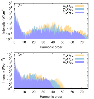
Figure 6: The HHG spectra with $\omega+2\omega$ frequency mixing for gapped graphene with $\Delta_{g}=2\ \mathrm{eV}$ in the strong-field regime for different relative polarizations of fundamental and SH pump fields. The electron-electron interaction is switched-off to avoid excitonic effects. (a) The fundamental frequency is $\omega=0.1\ \mathrm{eV}/\hbar$ and the field strength is taken to be $E_{01}=E_{02}=4\ \mathrm{MV/cm}$. (b) The fundamental frequency is $\omega=0.2\ \mathrm{eV}/\hbar$ and the field strength is taken to be $E_{01}=E_{02}=8\ \mathrm{MV/cm}$.

Comparing Fig. 6 with Figs. 3 and 4 we see that the general picture in considering regime for HHG is reverse, i.e. it is more preferable the parallel polarization case. For the atomic HHG this is explained by the three-step semiclassical recollision model. For gapped solid state system, HHG is similar to atomic one [4] and can be modeled based on the classical trajectory analysis of electron-hole pairs III.2. In this model interband HHG occurs through the laser induced tunneling or multiphoton creation of electron-hole pairs, which are accelerated in the laser field. When pairs re-encounter, they recombine and a harmonic photon is created. If the gap is considerably larger $\Delta_{g}>>\hbar\omega$ than the pump wave photon energy the tunneling is the main mechanism for creation of electron-hole pairs. Thus, electron-hole pairs are created near the minimum of the electron-hole energy $\mathcal{E}_{eh}\left(\mathbf{k}\right)$, i.e. near the Dirac points. For this case the particle distribution function $\mathcal{N}_{c}\left(\mathbf{k},t_{f}\right)$ after the interaction is shown in Fig. 7. As is expected, the creation of electron-hole pairs out of the Dirac points is exponentially suppressed, and the main contribution of electron-hole pairs are Dirac points, which correspond to pairs with approximately zero energy. It is also obvious that the tunneling probability will be larger for parallel polarization case. Besides, it is also clear that for orthogonally polarized two-color field to have re-encountering trajectories one needs electron-hole pairs created with both non-zero crystal momentum components, i.e. out of the Dirac points. The latter is suppressed for the gapped system. For graphene, due to the vanishing bandgap, all these conclusions do not hold, since the electron-hole pairs are created with nonzero energy and the main question remains: can we extend the semiclassical collision model for the considered case? The next subsection will be devoted to investigation of this problem.

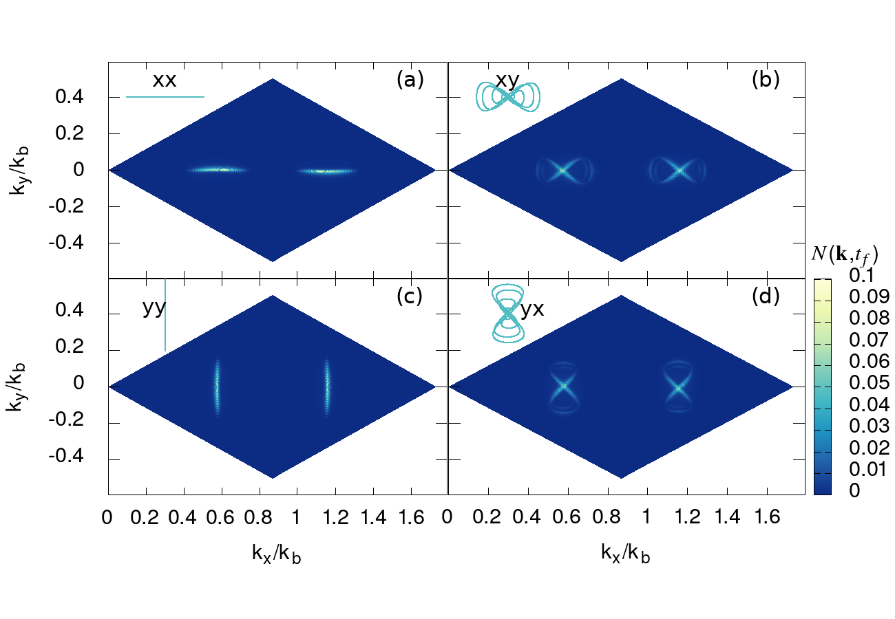
Figure 7: Particle distribution function $\mathcal{N}_{c}\left(\mathbf{k},t_{f}\right)$ after the interaction for gapped graphene with $\Delta_{g}=2\ \mathrm{eV}$, as a function of scaled dimensionless momentum components ($k_{x}/k_{b}$, $k_{y}/k_{b}$) for different relative polarizations of the fields. The electron-electron interaction is switched-off to avoid excitonic effects. The remaining parameters coresponds to the that of graphene.

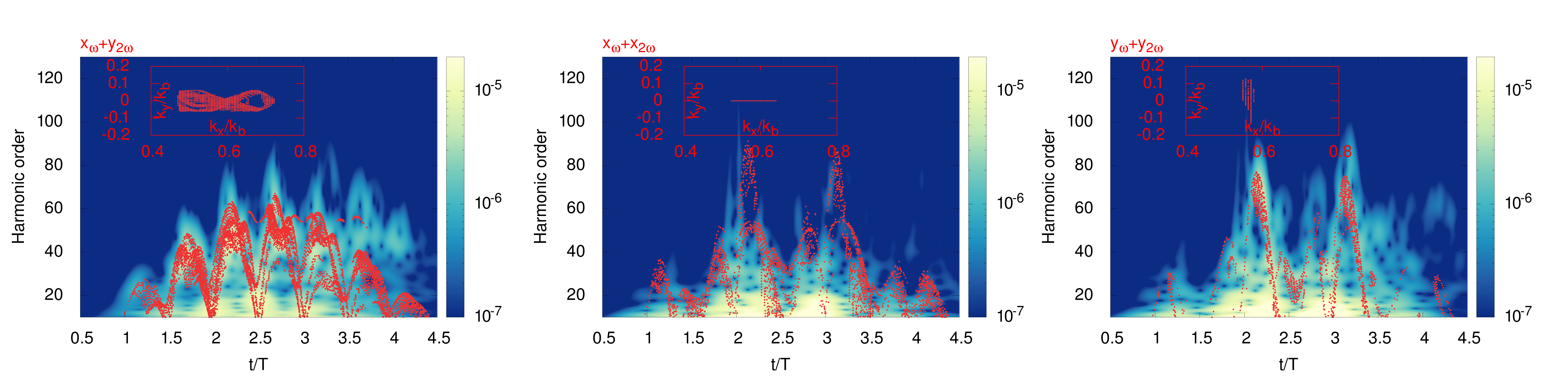
Figure 8: The spectrogram of the HHG process via the wavelet transform of the interband part of the surface current $\left|\mathbf{J}\left(t,\omega\right)\right|$ (colorbox in arbitrary units). The laser parameters are the same as in Fig. 3. The red dots over the spectrograms are the annihilation energies versus recollision times corresponding to the solutions of saddle point equations (26), (27 ), and (28). The insets for each case show the solutions of the saddle-point equations for crystal momenta obtained with the same resolution for half of the BZ.

III.2 Semiclassical Collision Model

To this end we need the evolution of high harmonic spectrum as a function of time, we perform the time-frequency analysis by means of the wavelet transform [78] of the interband part of the surface current:

$$J_{\alpha}\left(t,\overline{\omega}\right)=\sqrt{\frac{\overline{\omega}}{\sigma}}\int_{0}^{\tau}dt^{\prime}j_{e,\alpha}\left(t^{\prime}\right)e^{i\overline{\omega}\left(t^{\prime}-t\right)}e^{-\frac{\overline{\omega}^{2}}{2\sigma^{2}}\left(t^{\prime}-t\right)^{2}}.$$ (19)

We have chosen Morlet wavelet with $\sigma=4\pi$. The spectrogram of the HHG process via the wavelet transform of the interband part of the surface current $\left|\mathbf{J}\left(t,\overline{\omega}\right)\right|$ is shown in Fig. 8. The laser parameters are the same as in Fig. 3. In Fig. 8, for $x_{\omega}+y_{2\omega}$ case we have HHG emission peaks with period $0.5T$ starting at $t\approx 1.25T$ and ending at $4.25T$. These peaks coincide with the peaks of the vector potential, i.e. when the absolute value of the classical momentum given by the wave field is maximal. For the parallel polarization cases, the peaks also are near the peaks of the vector potential. This indicates that in some sense the above-obtained results can also be understood in the scope of the semiclassical collision model [4]. For this purpose, we now extend the semiclassical collision model to include graphene without applying Keldysh approximation [79] at $\mathcal{N}_{c}\ll 1$. Thus, the formal non explicit solution of Eq. (14) for the interband polarization can be written as:

$$\mathcal{P}(\mathbf{k}_{0},t)=\int_{0}^{t}dt^{\prime}e^{-\frac{i}{\hbar}S\left(\mathbf{k}_{0},t^{\prime},t\right)-\Gamma\left(t-t^{\prime}\right)}\mathcal{K}^{eh}\left(\mathbf{k}_{0},t^{\prime}\right),$$ (20)

where

$$S\left(\mathbf{k}_{0},t^{\prime},t\right)=\int_{t^{\prime}}^{t}\left[\mathcal{E}_{eh}\left(\mathbf{k}_{0}+\mathbf{A}\left(t^{\prime\prime}\right)\right)\right]dt^{\prime\prime}$$ (21)

is the classical action, and

$$\mathcal{K}^{eh}\left(\mathbf{k}_{0},t^{\prime}\right)=\frac{i}{\hbar}\left[\mathbf{E}\left(t^{\prime}\right)\mathbf{D}_{\mathrm{tr}}\left(\mathbf{k}_{0}+\mathbf{A}\left(t^{\prime}\right)\right)+\hbar\Omega_{c}\left(\mathbf{k}_{0}+\mathbf{A}\left(t^{\prime}\right)\right)\right]$$

$$\times\left[1-2\mathcal{N}_{c}(\mathbf{k}_{0}+\mathbf{A}\left(t^{\prime}\right),t^{\prime})\right]$$ (22)

is the electron-hole creation amplitude. The latter is maximal near the peaks of the total Rabi frequency and also includes the band filling factor $1-2N_{c}$, which reduces the electron-hole creation amplitude due to Pauli blocking. Taking into account the definition (15), the interband part of the surface current can be represented in the following form:

$$j_{e,\alpha}\left(t\right)=-\frac{2}{(2\pi)^{2}}\int_{BZ}d\mathbf{k}_{0}\int_{0}^{t}dt^{\prime}\mathcal{K}^{eh}\left(\mathbf{k}_{0},t^{\prime}\right)$$

$$\times\exp\left[-\frac{i}{\hbar}S\left(\mathbf{k}_{0},t^{\prime},t\right)-\Gamma\left(t-t^{\prime}\right)\right]\mathcal{A}_{\alpha}^{eh}\left(\mathbf{k}_{0},t\right)+\mathrm{c.c.},$$ (23)

which have a transparent physical interpretation in analogy with the atomic three-step model: electron-hole creation at $t^{\prime}$ with the amplitude $\mathcal{K}^{eh}\left(\mathbf{k}_{0},t^{\prime}\right)$, then propagation in the $BZ$, which is defined by the classical action (21). At that, the propagation amplitude is diminished because of damping. Finally, the electron-hole pair annihilates at $t$ with the amplitude

$$\mathcal{A}_{\alpha}^{eh}\left(\mathbf{k}_{0},t\right)=\mathrm{v}_{\mathrm{tr},\alpha}\left(\mathbf{k}_{0}+\mathbf{A}\left(t\right)\right).$$ (24)

For the Fourier transform of the interband current, we will have

$$j_{e,\alpha}\left(\overline{\omega}\right)=-\frac{2}{(2\pi)^{2}}\int_{0}^{\tau}dt\int_{BZ}d\mathbf{k}_{0}\int_{0}^{t}dt^{\prime}e^{-\Gamma\left(t-t^{\prime}\right)}\left[\mathcal{K}^{eh}\left(\mathbf{k}_{0},t^{\prime}\right)\right.$$

$$\left.\times\exp\left[-\frac{i}{\hbar}S\left(\mathbf{k}_{0},t^{\prime},t\right)+i\overline{\omega}t\right]\mathcal{A}_{\alpha}^{eh}\left(\mathbf{k}_{0},t\right)+\mathrm{c.c.}\right].$$ (25)

As is seen from this formula, the HHG can be driven by the nonlinearity of the transition velocities by which the annihilation amplitude (24) is defined, or by the fast oscillatory part stemming from the classical action. Assuming that the HHG is mainly driven by the last mechanism we can further extend the collision model evaluating integrals in Eq. (25) with the saddle point method. However, in contrast to the gapped system [79] one should relax the saddle point conditions for the following reasons: since the gap is zero, the electron and hole can be created with the initial energy ($\Delta_{\varepsilon}$) and due to the wave packet spreading annihilation can take place at relative distance $\rho_{0}$. Thus, we put the following conditions:

$$-\partial_{t^{\prime}}S<\Delta_{\varepsilon};\quad\left|\partial_{\mathbf{k}_{0}}S\right|<\rho_{0};\quad\partial_{t}S=\hbar\overline{\omega},$$

which give

$$\mathcal{E}_{eh}\left(\mathbf{k}_{0}+\mathbf{A}\left(t^{\prime}\right)\right)<\Delta_{\varepsilon},$$ (26)

$$\left|\Delta\mathbf{r}\right|<\rho_{0,}$$ (27)

$$\mathcal{E}_{eh}\left(\mathbf{k}_{0}+\mathbf{A}\left(t\right)\right)=\hbar\overline{\omega},$$ (28)

where

$$\Delta\mathbf{r=}\int_{t^{\prime}}^{t}\left[\mathbf{v}_{c}\left(\mathbf{k}_{0}+\mathbf{A}\left(t^{\prime\prime}\right)\right)-\mathbf{v}_{v}\left(\mathbf{k}_{0}+\mathbf{A}\left(t^{\prime\prime}\right)\right)\right]dt^{\prime\prime}$$ (29)

is the electron-hole separation vector and $\mathbf{v}_{c,v}=\hbar^{-1}\partial_{\mathbf{k}_{0}}\mathcal{E}_{c,v}\left(\mathbf{k}_{0}\right)$ are the group velocities. Saddle point equations (26), (27), and (28) have the following interpretation. The first one defines the birth time ($t^{\prime}$) at which the electron-hole pair is formed. It also states that the electron-hole pair is created with initial momentum defined by the area of the excited Fermi-Dirac sea. According to the second condition the laser accelerates the electron and hole with the instantaneous group velocities $\mathbf{v}_{c,v}$ and depending on the creation time the electron-hole may recollide at the time $t$ with final momentum $\mathbf{k}_{0}+\mathbf{A}\left(t\right)$ and relative distance $\rho_{0}$. The third condition is the conservation of energy: the electron-hole annihilate, emitting the energy in the form of a single photon. Taking into account Fig. 2, for $\Delta_{\varepsilon}$ we take $2\$eV and $\rho_{0}=2a$.

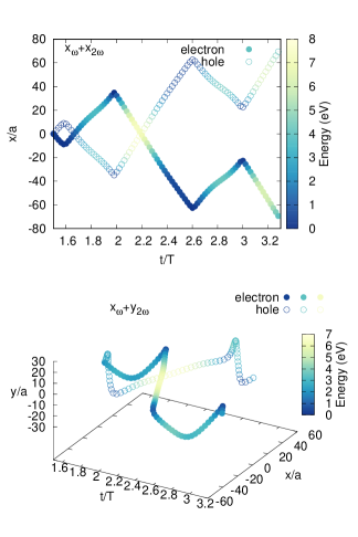
Figure 9: The colliding trajectories of an electron and a hole. (a) The electron (hole) is created at the $t_{c}=1.5T$ with the initial crystal momentum $k_{x}/k_{b}=0.57$ (-0.57), $k_{y}/k_{b}=0$(0) which corresponds to initial energy 0.3 eV. The colored trajectory and colored box show the energies acquired by carriers along the trajectory. (b) The electron (hole) is created at the $t_{c}=1.575T$ , with the initial crystal momentum $k_{x}/k_{b}=0.6$ ($-0.6$), $k_{y}/k_{b}=-0.05$ (0.05) which corresponds to initial energy 2 eV.

We then integrate the equation $\mathbf{r}_{e}\left(t^{\prime},t\right)\mathbf{=}\int_{t^{\prime}}^{t}\left[\mathbf{v}_{c}\left(\mathbf{k}_{0}+\mathbf{A}\left(t^{\prime\prime}\right)\right)\right]dt^{\prime\prime}$ to obtain the classical motion of the electron. Since we have electron-hole symmetry, for the hole we have $\mathbf{r}_{h}\left(t^{\prime},t\right)=-\mathbf{r}_{e}\left(t^{\prime},t\right)$. We also calculate the electron-hole distance $\rho\left(t^{\prime},t\right)=\left|\mathbf{r}_{e}-\mathbf{r}_{h}\right|$. It is assumed the colliding trajectories if at $t>t^{\prime}$ we have a local minimum of the electron-hole distance $\rho_{m}\left(t^{\prime},t\right)<\rho_{0}$. Then we fix the time and the corresponding energies $\mathcal{E}_{eh}\left(\mathbf{k}_{0}+\mathbf{A}\left(t\right)\right)$.

In Fig. 9 the typical colliding trajectories of an electron and a hole are shown. In Fig. 9(a) both fields are in the x-direction and we have one-dimensional motion. The electron-hole pair is created near the Dirac point. The laser field accelerates the electron and hole with the instantaneous group velocities $\mathbf{v}_{e}=-\mathbf{v}_{h}$. The colored trajectory and colored box show the energies acquired by carriers along the trajectory. We see two collisions: with the low energy $1.2\ \mathrm{eV}$ and the second one at $t=2.2T$ with the high energy $\mathcal{E}_{eh}\left(\mathbf{k}_{0}+\mathbf{A}\left(t\right)\right)/\hbar\omega\simeq 71$. In Fig. 9(b) wave fields are perpendicular to each other. In this case for the colliding trajectories, one needs electrons and holes created with both non-zero crystal momentum components. In this case we have two-dimensional motion. The electron-hole pair is created at the $t_{c}=1.575T$ with the initial energy $2.0\ \mathrm{eV}$ . Then, after the laser acceleration, the electron and hole collision/annihilation take place at $t_{a}=2.2T$. Here the collision is not perfect because of two- dimensional motion. The minimal distance is $0.6a$.

Varying the creation time $t^{\prime}$ from $0.5T$ to $4.5T$ we have solved Eqs. (26), (27), and (28). The corresponding annihilation/recombination energies versus recollision times are plotted in Fig. 8 over the spectrograms of the HHG process. As is seen from these plots, we have a fairly good agreement with fully quantum calculations.

The semiclassical approach has transparent physical interpretation in terms of Feynman’s path integral [80]. An infinite-dimensional functional integral is reduced to a coherent sum over the finite quantum trajectories defined by the saddle point equations [81, 82]. This way, Eq. (25) can be approximated as

$$j_{e,\alpha}\left(\overline{\omega}\right)\propto\sum_{\mathbf{k}_{0n},t_{n},t_{n}^{\prime}}A_{n}e^{-\Gamma\left(t_{n}-t_{n}^{\prime}\right)}\left[\mathcal{K}^{eh}\left(\mathbf{k}_{0n},t_{n}^{\prime}\right)\right.$$

$$\left.\times\exp\left[-\frac{i}{\hbar}S\left(\mathbf{k}_{0n},t_{n}^{\prime},t_{n}\right)+i\overline{\omega}t_{n}\right]\mathcal{A}_{\alpha}^{eh}\left(\mathbf{k}_{0n},t_{n}\right)+\mathrm{c.c.}\right].$$ (30)

where $\mathbf{k}_{0n},t_{n},t_{n}^{\prime}$ are the solutions of the saddle point equations (26)-(28), $A_{n}$ is an amplitude and $S$ is defined in (21). One obtains qualitatively and quantitatively different results depending on how many and which trajectories are involved in Eq. (30). The insets in Fig. 8 for each case show the solutions of the saddle-point equations for crystal momenta obtained with the same resolution for half of BZ. Note that for each solution $\mathbf{k}_{0n}$ there may be several trajectories that can interfere constructively or destructively in Eq. (30) depending on the phase factor. In the case of an orthogonally polarized two-color field, the crystal momenta obeying saddle point equations (26)-(28) and, consequently, the trajectories are an order of magnitude larger than in the case of parallel polarization, cf. Fig. 8. At that, a large number of trajectories with the different $\mathbf{k}_{0n}$ but the close $t_{n}^{\prime},t_{n}$ considerably enlarges the number of constructively interfering terms in Eq. ( 30). For this reason, $j_{e,\alpha}\left(\overline{\omega}\right)$ enhances in an orthogonally polarized two-color field. For the gapped system this favorable condition disappears. Thus, the saddle point equation (26) that defines the birth time ($t^{\prime}$) becomes $E_{eh}\left(\mathbf{k}_{0}+\mathbf{A}\left(t^{\prime}\right)\right)\approx-\Delta_{g}$, which cannot be satisfied for any real time. Because of the imaginary solution $t^{\prime}$, we have an exponential suppression of the probability of electron and hole production, especially with momenta outside the Dirac points. In addition, tunneling occurs near the maxima of the electric field strength [79] and is more probable for parallel polarization of a two-color field (1). These are the main reasons why in the gapped nanostructure HHG in an orthogonally polarized two-color field is suppressed compared with the case of parallel polarization. Also, note that for the observation of the HHG yield in the orthogonally polarized two-color field the incident intensity of SH wave should be comparable to or larger than the incident fundamental wave intensity to ensure the existence of re-encountering trajectories Eq. (27), which maximize the recombination probability.

IV Conclusion

We have presented the microscopic theory of nonlinear interaction of a monolayer graphene with a strong bichromatic few-cycle driving pulse that is composed of the superposition of an infrared fundamental pulse of linear polarization and its second harmonic at the parallel and orthogonal polarizations. The electron-electron Coulomb interaction has been taken into account in the scope of HF approximation beyond the Dirac cone approximation, which is applicable to the full Brillouin zone of the hexagonal tight-binding nanostructure. The obtained results show that in all cases we have an overall enhancement of HHG yield compared with the independent charged carrier model due to the electron-hole attractive interaction. We have shown that in the case of the orthogonally polarized two-color field the generated high-harmonics are stronger than those obtained in the parallel polarization case by more than two orders of magnitude. This enhancement is colossal mainly for the interband part of HHG that is predominant for the plateau part of the spectrum. This tendency persists for a wide range of intensities and frequencies of driving waves. The physical origin of polarization-dependent strong enhancement in graphene is also deduced from the three-step semiclassical electron-hole collision model, extended to graphene with pseudo-relativistic energy dispersion and without Keldysh approximation.

Appendix A The single-particle Hamiltonian and other derived quantities

In this section we consider the details of the single particle Hamiltonian and give concrete expressions for the used physical quantities. The single particle Hamiltonian is taken to be:

$$\widehat{H}=\left[\begin{array}[]{cc}0&-\gamma_{0}f\left(\mathbf{k}\right)\\ -\gamma_{0}f^{\ast}\left(\mathbf{k}\right)&0\end{array}\right],$$ (31)

where $\gamma_{0}=2.8\$eV. The structure function is

$$f\left(\mathbf{k}\right)=e^{i\frac{ak_{y}}{\sqrt{3}}}+2e^{-i\frac{ak_{y}}{2\sqrt{3}}}\cos\left(\frac{ak_{x}}{2}\right),$$ (32)

where $a$ is the lattice spacing. The reciprocal lattice unit cell is a rhombus formed by   two vectors:

$$\mathbf{b}_{1}=\left(\frac{2\pi}{a},-\frac{2\pi}{a\sqrt{3}}\right),\quad\mathbf{b}_{2}=\left(\frac{2\pi}{a},\frac{2\pi}{a\sqrt{3}}\right).$$ (33)

The low-energy excitations are centered around the two points $\mathrm{K}_{+}$ and $\mathrm{K}_{-}$represented by the vectors

$$\mathbf{K}_{+}=\frac{k_{b}}{\sqrt{3}}\widehat{\mathbf{x}},\quad\mathbf{K}_{-}=\frac{2k_{b}}{\sqrt{3}}\widehat{\mathbf{x}},$$ (34)

where $k_{b}=4\pi/\sqrt{3}a$ . Note that near the two Dirac points $\gamma_{0}f\left(\mathbf{k}\right)=i\mathrm{v}_{F}\hbar k_{y}\mp\mathrm{v}_{F}\hbar k_{x}$, where $\mathrm{v}_{F}=\sqrt{3}a\gamma_{0}/2\hbar$ is the Fermi velocity. The eigenstates of the Hamiltonian (31) are

$$|\lambda,\mathbf{k}\rangle=\frac{1}{\sqrt{2}}\left[\begin{array}[]{c}-\frac{f\left(\mathbf{k}\right)}{\left|f\left(\mathbf{k}\right)\right|}\\ \lambda\end{array}\right],$$ (35)

corresponding to energies

$$\mathcal{E}_{\lambda}\left(\mathbf{k}\right)=\lambda\gamma_{0}\left|f\left(\mathbf{k}\right)\right|.$$ (36)

Here the band index $\lambda=\pm 1$ (for conduction ($\lambda=1$) and valence ($\lambda=-1$) bands). The transition dipole moment is explicitly given by

$$\mathbf{D}_{\mathrm{tr}}\left(\mathbf{k}\right)=-\frac{ea}{2\left|f\left(\mathbf{k}\right)\right|^{2}}\sin\left(\frac{\sqrt{3}}{2}ak_{y}\right)\sin\left(\frac{ak_{x}}{2}\right)\widehat{\mathbf{x}}$$

$$+\frac{ea}{2\sqrt{3}\left|f\left(\mathbf{k}\right)\right|^{2}}\left(\cos\left(ak_{x}\right)-\cos\left(\frac{\sqrt{3}}{2}ak_{y}\right)\cos\left(\frac{ak_{x}}{2}\right)\right)\widehat{\mathbf{y}}.$$ (37)

The band velocity is given by the formula

$$\mathbf{v}_{c}\left(\mathbf{k}\right)=-\mathrm{v}_{F}\frac{2}{\sqrt{3}\left|f\left(\mathbf{k}\right)\right|}$$

$$\times\left[\cos\left(\frac{\sqrt{3}}{2}ak_{y}\right)\sin\left(\frac{ak_{x}}{2}\right)+\sin\left(ak_{x}\right)\right]\widehat{\mathbf{x}}$$

$$-\mathrm{v}_{F}\frac{2}{\left|f\left(\mathbf{k}\right)\right|}\sin\left(\frac{\sqrt{3}}{2}ak_{y}\right)\cos\left(\frac{ak_{x}}{2}\right)\widehat{\mathbf{y}}.$$ (38)

For the gapped graphene we used general formulas [83] taking also into account Berry connections.

References

- [1] S. Ghimire, A. D. DiChiara, E. Sistrunk, P. Agostini, L. F. DiMauro, and D. A. Reis, Nature Phys. 7, 138 (2011).
- [2] B. Zaks, R.-B. Liu, and M. S. Sherwin, Nature 483, 580 (2012).
- [3] O. Schubert, M. Hohenleutner, F. Langer, B. Urbanek, C. Lange, U. Huttner, D. Golde, T. Meier, M. Kira, S. W. Koch, and R. Huber, Nature Photon. 8, 119 (2014).
- [4] G. Vampa, T. J. Hammond, N. Thire, B. E. Schmidt, F. Legare, C. R. McDonald, T. Brabec, and P. B. Corkum, Nature 522, 462 (2015).
- [5] T. T. Luu, M. Garg, S. Yu. Kruchinin, A. Moulet, M. Th. Hassan, and E. Goulielmakis Nature 521, 498 (2015).
- [6] M. Hohenleutner, F. Langer, O. Schubert, M. Knorr, U. Huttner, S. W. Koch, M. Kira, and R. Huber, Nature 523, 572 (2015).
- [7] Y. S. You, D. A. Reis, S. Ghimire, Nat. Phys. 13, 345 (2016).
- [8] F. Langer, M. Hohenleutner, C. P. Schmid, C. Poellmann, P. Nagler, T. Korn, C. Schüller, M. S. Sherwin, U. Huttner, J. T. Steiner, S. W. Koch, M. Kira, R. Huber, Nature 533, 225 (2016)
- [9] S. Ghimire, D. A. Reis, Nat. Phys. 15, 10 (2019).
- [10] A. J. Uzan, G. Orenstein, A. Jimenez-Galan, C. McDonald, R. E. F. Silva, B. D. Bruner, N. D. Klimkin, V. Blanchet, T. Arusi-Parpar, M. Kruger et al., Nat. Photonics 14, 183 (2020).
- [11] P. Bowlan, E. Martinez-Moreno, K. Reimann, T. Elsaesser, and M. Woerner, Phys. Rev. B 89, 041408(R) (2014).
- [12] N. Yoshikawa, T.Tamaya, K. Tanaka, Science 356, 736 (2017).
- [13] H. A. Hafez et al., Nature 561, 507 (2018).
- [14] F. Giorgianni et al., Nat. Commun. 7, 11421 (2016).
- [15] G. Le Breton, A. Rubio, N. Tancogne-Dejean, Phys. Rev. B 98, 165308 (2018).
- [16] H. Liu, Y. Li, Y.S. You, S. Ghimire, T. F. Heinz, and D. A. Reis, Nat. Phys. 13, 262 (2017).
- [17] Y. S. You, Y. Yin, Y. Wu, A. Chew, X. Ren, F. Zhuang, S. Gholam-Mirzaei, M. Chini, Z. Chang, Nat. Commun. 8, 724 (2017).
- [18] T. T. Luu, Z. Yin, A. Jain, T. Gaumnitz, Y. Pertot, J. Ma, and H. J. Wörner, Nat. Commun. 9, 3723 (2018).
- [19] H. K. Avetissian, Relativistic Nonlinear Electrodynamics: The QED Vacuum and Matter in Super-Strong Radiation Fields (Springer, Berlin 2015).
- [20] O. Smirnova, Y. Mairesse, S. Patchkovskii, N. Dudovich, D. Villeneuve, P. Corkum, M. Yu. Ivanov, Nature 460, 972 (2009).
- [21] H. Lakhotia, H. Y. Kim, M. Zhan, S. Hu, S. Meng, and E. Goulielmakis, Nature 583, 55 (2020).
- [22] R. E. F. Silva, I. V. Blinov, A. N. Rubtsov, O. Smirnova, M. Ivanov, Nat. Photonics 12, 266 (2018).
- [23] D. Bauer and K. K. Hansen, Phys. Rev. Lett. 120, 177401 (2018).
- [24] G. Vampa, T. J. Hammond, N. Thiré, B. E. Schmidt, F. Légaré, C. R. McDonald, T. Brabec, D. D. Klug, and P. B. Corkum, Phys. Rev. Lett. 115, 193603 (2015).
- [25] N. Tancogne-Dejean, O. D. Mucke, F. X. Kartner, and A. Rubio, Phys. Rev. Lett. 118, 087403 (2017).
- [26] T. T. Luu, H. J.Worner, Nat. Commun. 9, 916 (2018).
- [27] P. B. Corkum, Phys. Rev. Lett. 71, 1994 (1993).
- [28] P. B. Corkum and F. Krausz, Nat. Phys. 3, 381 (2007).
- [29] F. Krausz, and M. Ivanov, Rev. Mod. Phys. 81, 163 (2009).
- [30] S. A. Mikhailov, K. Ziegler, J. Phys. Condens. Matter 20, 384204 (2008).
- [31] H. K. Avetissian, A. K. Avetissian, G. F. Mkrtchian, Kh. V. Sedrakian, Phys. Rev. B 85, 115443 (2012).
- [32] H. K. Avetissian, G. F. Mkrtchian, K. G. Batrakov, S. A. Maksimenko, A. Hoffmann, Phys. Rev. B 88, 165411 (2013).
- [33] P. Bowlan, E. Martinez-Moreno, K. Reimann, T. Elsaesser, and M. Woerner, Phys. Rev. B 89, 041408(R) (2014).
- [34] I. Al-Naib, J. E. Sipe, and M. M. Dignam, Phys. Rev. B 90, 245423 (2014).
- [35] I. Al-Naib, J. E. Sipe, and M. M. Dignam, New J. Phys. 17, 113018 (2015).
- [36] L. A. Chizhova, F. Libisch, and J. Burgdorfer, Phys. Rev. B 94, 075412 (2016).
- [37] H. K. Avetissian, G. F. Mkrtchian, Phys. Rev. B 94, 045419 (2016).
- [38] L. A. Chizhova, F. Libisch, and J. Burgdorfer, Phys. Rev. B 95, 085436 (2017).
- [39] D. Dimitrovski, L. B. Madsen, and T. G. Pedersen, Phys. Rev. B 95, 035405 (2017).
- [40] H. K. Avetissian and G. F. Mkrtchian, Phys. Rev. B 97, 115454 (2018).
- [41] S. A. Sato, H. Hirori, Y. Sanari, Y. Kanemitsu, and A. Rubio, Phys. Rev. B 103, L041408 (2021).
- [42] Ó. Zurrón-Cifuentes, R. Boyero-García, C. Hernández-García, A. Picón, L. Plaja, Optics express 27, 7776 (2019).
- [43] M. S. Mrudul and G. Dixit, Phys. Rev. B 103, 094308 (2021).
- [44] Y. Zhang, L. Li, J. Li, T. Huang, P. Lan, P. Lu, Phys. Rev. A 104, 033110 (2021).
- [45] F. Dong, Q. Xia, J. Liu, Phys. Rev. A 104, 033119 (2021).
- [46] H. Eichmann, A. Egbert, S. Nolte, C. Momma, B. Wellegehausen, W. Becker, S. Long, and J. K. McIver, Phys. Rev. A 51, R3414 (1995).
- [47] Y. Oishi, M. Kaku, A. Suda, F. Kannari, K. Midorikawa, Optics express, 14, 7230 (2006).
- [48] S. Watanabe, K. Kondo, Y. Nabekawa, A. Sagisaka, and Y. Kobayashi, Phys. Rev. Lett. 73, 2692 (1994).
- [49] J.-B. Li, X. Zhang, S.-J. Yue, H.-M. Wu, B.-T. Hu, and H.-C. Du, Opt. Express 25, 18603 (2017).
- [50] T. T. Luu and H. J. Worner, Phys. Rev. A 98, 041802(R) (2018).
- [51] H. Shirai, F. Kumaki, Y. Nomura, and T. Fuji, Opt. Lett. 43, 2094 (2018).
- [52] X. Song, S. Yang, R. Zuo, T. Meier, and W. Yang, Phys. Rev. A 101, 033410 (2020).
- [53] T.-J. Shao, L.-J. Lu, J.-Q. Liu, and X.-B. Bian, Phys. Rev. A 101, 053421 (2020).
- [54] F. Navarrete and U. Thumm, Phys. Rev. A 102, 063123 (2020).
- [55] M. S. Mrudul, Alvaro Jimenez-Galan, M. Ivanov, and G. Dixit, Optica 8, 422 (2021).
- [56] J.-Y. Yan, Phys. Rev. B 78, 075204 (2008).
- [57] J.A. Crosse, R.B. Liu, Phys. Rev. B 89, 121202(R) (2014).
- [58] X.T. Xie, B. F. Zhu, R. B. Liu, New J. Phys. 15, 105015 (2018).
- [59] F. Langer, M. Hohenleutner, C. P. Schmid, C. Poellmann, P. Nagler, T. Korn, C. Schüller, M. S. Sherwin, U. Huttner, J. T. Steiner, S. W. Koch, M. Kira, R. Huber, Nature 533, 225 (2016)
- [60] F. Langer, C. P. Schmid, S. Schlauderer, M. Gmitra, J. Fabian, P. Nagler, C. Schüller, T. Korn, P. G. Hawkins, J. T. Steiner, U. Huttner, S. W. Koch, M. Kira, R. Huber, Nature 557, 76 (2018).
- [61] H. K. Avetissian, A. K. Avetissian, B. R. Avchyan, G. F. Mkrtchian, Phys. Rev. B 100, 035434 (2019).
- [62] H. K. Avetissian, G. F. Mkrtchian, and K. Z. Hatsagortsyan, Phys. Rev. Research 2, 023072 (2020).
- [63] M. Breusing, S. Kuehn, T. Winzer, E. Malić, F. Milde, N. Severin, J. P. Rabe, C. Ropers, A. Knorr, and T. Elsaesser, Phys. Rev. B 83, 153410 (2011).
- [64] E. Malic, T. Winzer, E. Bobkin, A. Knorr, Phys. Rev. B 84, 205406 (2011).
- [65] E. Malic, A. Knorr, Graphene and carbon nanotubes: ultrafast optics and relaxation dynamics (John Wiley & Sons, 2013).
- [66] M. Kira, S. W. Koch, Semiconductor Quantum Optics (Cambridge University Press, Cambridge, 2012).
- [67] L. Meitner, Z. Physik 9, 145 (1922).
- [68] P. Auger, C.R. Acad. Sci. F 177, 169 (1923).
- [69] S. Dong et al, arXiv preprint arXiv:2108.06803 (2021).
- [70] S. Guazzotti, A. Pusch, D. E. Reiter, and O. Hess, Phys. Rev. B 94, 115303 (2016).
- [71] L. Yang, J. Deslippe, C.-H. Park, M. L. Cohen, and S. G. Louie, Phys. Rev. Lett. 103, 186802 (2009).
- [72] K. F. Mak, J. Shan, and T. F. Heinz, Phys. Rev. Lett. 106, 046401 (2011).
- [73] W. V. Houston, Phys. Rev. 57, 184 (1940).
- [74] J. Li, X. Zhang, S. Fu, Y. Feng, B. Hu, and H. Du, Phys. Rev. A 100, 043404 (2019).
- [75] A. Roberts, D. Cormode, C. Reynolds, Ty Newhouse-Illige, B. J. LeRoy, and A. S. Sandhu, Appl. Phys. Lett. 99, 051912 (2011).
- [76] C. Heide, T. Higuchi, H. B. Weber, and P. Hommelhoff, Phys. Rev. Lett. 121, 207401 (2018).
- [77] X. Liu, X. Zhu, L. Li, Y. Li, Q. Zhang, P. Lan, and P. Lu, Phys. Rev. A 94, 033410 (2016).
- [78] X. M. Tong, Shih-I Chu, Phys. Rev. A 61, 021802(R) (2000).
- [79] L. V. Keldysh, J. Exp. Theor. Phys. 47, 1945 (1964) [Sov. Phys. JETP 20, 1307 (1965)].
- [80] P. Salières, B. Carré, L. Le Déroff, F. Grasbon, G. G. Paulus, H. Walther, R. Kopold, W. Becker, D. B. Milošević, A. Sanpera, and M. Lewenstein, Science 292, 902 (2001).
- [81] G. Vampa, C. R. McDonald, G. Orlando, D. D. Klug, P. B. Corkum and T. Brabec, Phys. Rev. Lett. 113, 073901 (2014).
- [82] L. Li, P. Lan, X. Zhu, T. Huang, Q. Zhang, M. Lein, and P. Lu, Phys. Rev. Lett. 122, 193901 (2019).
- [83] H. K. Avetissian and G. F. Mkrtchian, Phys. Rev. B 99, 085432 (2019).