$P_{1}$–Nonconforming Quadrilateral Finite Element Space with Periodic Boundary Conditions:
Part II. Application to the Nonconforming Heterogeneous Multiscale Method

Abstract

A homogenization approach is one of effective strategies to solve multiscale elliptic problems approximately. The finite element heterogeneous multiscale method (FEHMM) which is based on the finite element makes possible to simulate such process numerically. In this paper we introduce a FEHMM scheme for multiscale elliptic problems based on nonconforming spaces. In particular we use the noconforming element with the periodic boundary condition introduced in the companion paper. Theoretical analysis derives a priori error estimates in the standard Sobolev norms. Several numerical results which confirm our analysis are provided.

65N30

1 Introduction

The finite element method (FEM) is one of the successful methods to approximate the solution of partial differential equations derived in various fields of studies. However it has a drawback when we treat a problem containing coefficient tensors with heterogeneity. For instance, when the coefficient is highly oscillatory in micro scale, it is necessary to consider a sufficiently refined mesh consisting of elements comparable with the micro scale in order to get a numerical solution which is sufficiently close to the exact solution. Such a refinement increases the number of unknowns in the system of equations we set to solve, which is a critical burden for numerical simulation. In these decades, several efficient multiscale methods have been developed to overcome this shortage of the standard FEM. Among them, we refer to numerical homogenization [7, 8, 25, 27], MsFEM (multiscale finite element methods) and GMsFEM (generalized MsFEM) [23, 21, 22, 24, 28, 29], VMS (variational multiscale finite element methods) [32], MsFVM (multiscale finite volume methods) [33] and HMM (heterogeneous multiscale methods) [6, 19].

Most of the works cited above are based on the conforming finite element framework, while nonconforming finite elements have prominence for their numerical stability especially in solving incompressible fluid flows [13, 14, 16, 35, 45, 49], nearly incompressible elastic materials [10, 36], and biharmonic problems [40, 30, 31, 39, 44, 47]. We remark that the first nonconforming analysis in multiscale methods has been done by Efendiev et al. in [26] in order to analyze the nonconforming nature where conforming finite elements were adopted with oversampling. Recently Lozinski et al. began to develop the idea of using the Crouzeix–Raviart element [16] in multiscale finite element methods intensively for elliptic and Stokes problems [11, 38, 12]. Especially it has been shown that in applying the Crouzeix–Raviart nonconforming multiscale finite element for perforated domains the use of carefully–chosen extra bubble elements improves stability and efficiency substantially [41, 17]. In the generalized MsFEM direction, Lee and Sheen [37] introduced the general framework for applying the nonconforming concept to elliptic problems.

In the introduction of the FEHMM (Finite Element HMM), the standard (conforming) finite element spaces have been employed for the micro and macro function space (see, for instance, [1], and the references therein), various types of finite element spaces being adopted since then. The discontinuous Galerkin (DG) approach is introduced to impose the continuity of numerically homogenized jump across adjacent faces [2]. A posteriori error estimates and corresponding adaptive approaches for the FEHMM are proposed [5]. The generalized FEHMM approach by introduction of the on-line and off-line space [3].

The aim of this paper is to attempt to apply the nonconforming approach to the primitive HMM for elliptic problems rigorously, leaving the extension of the nonconforming approach as future works to generalized HMMs and to more practical fluid and solid mechanical problems, where the numerical stability is easily achievable owing to the nature of nonconformity of elements. In particular, in this paper we employ the $P_{1}$–NC quadrilateral element [43, 42], which will share the same nature as the lowest–order Crouzeix–Raviart element since it contains only linear polynomials in each rectangles or hexahedrons. We would like to highlight that the use of rectangular–type element has an extra advantage over the simplicial elements in the application of multiscale methods, not to mention the simplicity of constructing elements in three dimension, but the suitability of rectangular type elements in dealing with periodicity. In addition, by employing the $P_{1}$–NC quadrilateral element we do not need any additional linearization step for macro constraint functions in solving micro problems on sampling domains, since the $P_{1}$–NC quadrilateral element is already linear. This is another main advantage of our approach over using the conforming bilinear element. See Remark 3.2.

This paper is organized as follows. In Section 2 we state in brief preliminaries and notations to be used later. We introduce a nonconforming finite element heterogeneous multiscale method based on nonconforming spaces in Section 3. Section 4 is devoted to prove the main theorems for a priori error estimates of our proposed method. We give several numerical examples and results in Section 5.

2 Preliminaries

Let $\Omega\subset\mathbb{R}^{d},d=2,3,$ be a bounded domain with $C^{\infty}$ boundary $\partial\Omega$. Denote $\mathbf{x}=(x_{1},\cdots,x_{d})^{t}\in\mathbb{R}^{d}$. Consider a multiscale elliptic problem

(1a) $$-\nabla\cdot\Big{(}\mathbf{A}^{\varepsilon}({\bf x})\nabla u^{\varepsilon}({\bf x})\Big{)} =f({\bf x})\quad\mbox{in }\Omega,$$

(1b) $$u^{\varepsilon} =0\quad\quad\ \mbox{on }\partial\Omega,$$

where $\varepsilon\ll 1$ is a scale parameter. Here, the coefficient tensor $\mathbf{A}^{\varepsilon}\in[L^{\infty}(\Omega)]^{d\times d}$ is assumed to be symmetric, uniformly elliptic and bounded, i.e., there exist $\lambda>0$ and $\Lambda>0$ which do not depend on ${\bf x}$ such that $\lambda|\xi|^{2}\leq\xi^{t}\mathbf{A}^{\varepsilon}({\bf x})\ \xi\leq\Lambda|\xi|^{2}$ for all $\xi\in\mathbb{R}^{d}$.

2.1 Homogenization

Denote by $Y=\prod_{k=1}^{d}[0,\ell_{k}]$ be a period cell for fixed $0<\ell_{k},k=1,\cdots,d.$ Let $\mathbf{A}(\cdot,\cdot):\mathbb{R}^{d}\times\mathbb{R}^{d}\rightarrow\mathbb{R}^{d\times d}$ be a $Y$-periodic function with respect to the second variable, i.e., $\mathbf{A}({\mathbf{x}},{\mathbf{y}})=\mathbf{A}({\mathbf{x}},{\mathbf{y}}+\ell_{k}{\mathbf{e}}_{k})$ for $1\leq k\leq d,$ where $\mathbf{e}_{j}$ denotes the $j$–th standard unit vector in $\mathbb{R}^{d}.$ Assume that $\mathbf{A}^{\varepsilon}({\mathbf{x}}):=\mathbf{A}({\mathbf{x}},{\mathbf{x}}/\varepsilon).$ Then, the following result is well–known [15, 34, 46].

Theorem 2.1 (Periodic case).

Suppose that $\mathbf{A}^{\varepsilon}({\mathbf{x}}):=\mathbf{A}({\mathbf{x}},{\mathbf{x}}/\varepsilon)$ where $\mathbf{A}({\mathbf{x}},{\mathbf{y}})$ is $Y$-periodic for the variable ${\mathbf{y}}=(y_{1},\cdots,y_{d})$. Let $f\in L^{2}(\Omega)$. Then there exists a homogenized coefficient tensor $\mathbf{A}^{0}$ such that

$$\left\{\begin{aligned} &u^{\varepsilon}\rightharpoonup u^{0}\mbox{ weakly in }H^{1}_{0}(\Omega),\\ &\mathbf{A}^{\varepsilon}\nabla u^{\varepsilon}\rightharpoonup\mathbf{A}^{0}\nabla u^{0}\mbox{ weakly in }[L^{2}(\Omega)]^{d},\end{aligned}\right.$$

where $u^{0}$ is a unique solution in $H^{1}_{0}(\Omega)$ of the homogenized problem:

(2) $$\left\{\begin{aligned} -\nabla\cdot\Big{(}\mathbf{A}^{0}({\mathbf{x}})\nabla u^{0}({\mathbf{x}})\Big{)}&=f({\mathbf{x}})\quad\mbox{in }\Omega,\\ u^{0}&=0\quad\quad\ \mbox{on }\partial\Omega.\end{aligned}\right.$$

In fact, the homogenized coefficient $\mathbf{A}^{0}=(A^{0}_{ij})$ is given by

$$A^{0}_{ij}({\mathbf{x}})=\frac{1}{|Y|}\int_{Y}\Big{(}A_{ij}({\mathbf{x}},{\mathbf{y}})+\sum_{k=1}^{d}A_{ik}({\mathbf{x}},{\mathbf{y}})\frac{\partial\chi^{j}}{\partial y_{k}}\Big{)}\kern 0.43057pt\operatorname{d\mathbf{y}},$$

where $|Y|$ denotes the volume of $Y$, and $\chi^{j}=\chi^{j}({\mathbf{x}},{\mathbf{y}})$ the solution of the cell problem:

$$\left\{\begin{aligned} &-\nabla_{\mathbf{y}}\cdot\left(\mathbf{A}({\mathbf{x}},{\mathbf{y}})\nabla_{\mathbf{y}}\chi^{j}\right)=\nabla_{\mathbf{y}}\cdot\left(\mathbf{A}({\mathbf{x}},{\mathbf{y}})\ {\mathbf{e}}_{j}\right)\quad\mbox{in }Y,\\ &\chi^{j}\mbox{ is $Y$-periodic},\\ &\int_{Y}\chi^{j}\kern 0.43057pt\operatorname{d\mathbf{y}}=0.\end{aligned}\right.$$

2.2 Some notations

Let $D$ be a bounded open domain in $\mathbb{R}^{d},d=2,3$. Denote by $L^{2}(D),$ $H^{1}(D),$ and $H^{1}_{0}(D)$ the standard Sobolev spaces on $D$ with the standard Sobolev norms $\|\cdot\|_{0,D}$, $\|\cdot\|_{1,D}$, and (semi-)norm $|\cdot|_{1,D}$, respectively. By $C^{\infty}_{\#}(D)$ designate the set of $Y$–periodic $C^{\infty}$ functions on $D$ and by $H^{1}_{\#}(D)$ the closure of $C^{\infty}_{\#}(D)$ with respect to the norm $\|\cdot\|_{1,D}$ in $H^{1}(D)$. $\widetilde{H}^{1}_{\#}(D)$ is a subspace of $H^{1}_{\#}(D)$ which consists of functions whose mean values on $D$ are zero. We will mean by $(\cdot,\cdot)_{D}$ the $L^{2}(D)$ inner product. In the case of $D=\Omega$, the subscript $D$ on notations of norms and inner product is omitted. For $d-1$ dimensional face $\tau$, $\left\langle\cdot,\cdot\right\rangle_{\tau}$ indicates the $L^{2}(\tau)$ inner product.

By $|D|$ we denote the volume of the domain $D$. For an integrable function $v\in L^{1}(D)$, the mean value on $D$ is denoted by $\mathop{\ooalign{$\int$\cr$-$}}_{D}v=\frac{1}{|D|}\int_{D}v.$ Throughout this paper $C$ denotes a generic constant and its value varies depending on the position where it appears.

Consider a family of triangulations ${\mathcal{T}}_{h}=({\mathcal{T}}_{h}(D))_{0<h<1}$ for the domain $D$ consisting of quadrilateral elements. Let $\mathcal{F}_{h}^{i},\mathcal{F}_{h}^{b},$ and $\mathcal{F}_{h}^{b,opp}$ denote the sets of all interior faces, of all boundary faces, and of all pairs consisting of two boundary faces on opposite position of each period cell $Y$ in ${\mathcal{T}}_{h}$, respectively. Set $\mathcal{F}_{h}=\mathcal{F}_{h}^{i}\cup\mathcal{F}_{h}^{b}.$

Set

$$V_{h}^{P_{1}}(D) =\Big{\{}v\in L^{2}(D)~{}\Big{|}~{}\left.v\right|_{K}\in\mathcal{P}_{1}(K)\quad\forall K\in{\mathcal{T}}_{h}(D),\ \left\langle[v]_{\tau},1\right\rangle_{\tau}=0\quad\forall\tau\in\mathcal{F}_{h}^{i}\Big{\}},$$

$$V_{h,0}^{P_{1}}(D) =\Big{\{}v\in V_{h}^{P_{1}}(D)~{}\Big{|}~{}\left\langle v,1\right\rangle_{\tau}=0\quad\forall\tau\in\mathcal{F}_{h}^{b}\Big{\}},$$

$$V_{h,\#}^{P_{1}}(D) =\Big{\{}v\in V_{h}^{P_{1}}(D)~{}\Big{|}~{}\left\langle v,1\right\rangle_{\tau_{1}}=\left\langle v,1\right\rangle_{\tau_{2}}\quad\forall(\tau_{1},\tau_{2})\in\mathcal{F}_{h}^{b,opp},\ (v,1)_{D}=0\Big{\}},$$

where $\mathcal{P}_{1}(K)$ denotes the set of linear polynomials on $K$, and $[\cdot]_{\tau}$ the jump across face $\tau$. Let $|\cdot|_{1,h,D}$ denote the mesh-dependent broken energy norm on $V_{h}^{P_{1}}(D)$, i.e., $|v|_{1,h,D}=\big{[}\sum_{K\in{\mathcal{T}}_{h}(D)}\|\nabla v\|_{0,K}^{2}\big{]}^{1/2}.$ The nonconforming Galerkin method for (2) reads as: find $u_{h}^{0}\in V_{h,0}^{P_{1}}(\Omega)$ such that

(3) $$\sum_{K\in{\mathcal{T}}_{h}(\Omega)}(\mathbf{A}^{0}\nabla u_{h}^{0},\nabla v_{h})=(f,v_{h}),\quad v_{h}\in V_{h,0}^{P_{1}}(\Omega).$$

The standard error analysis for nonconforming elements implies the following a priori error estimate, see [43, 18],

(4) $$|u^{0}_{h}-u^{0}|_{1,h,\Omega}\leq Ch|u^{0}|_{2}.$$

3 FEHMM based on nonconforming spaces

In this section we introduce a FEHMM scheme based on nonconforming finite spaces for the multiscale elliptic problem (1). We follow the framework of FEHMM [1, 2] with slight modification for nonconforming function spaces. Let ${\mathcal{T}}_{H}:={\mathcal{T}}_{H}(\Omega)$ be a regular triangulation of $\Omega$ with quasi-uniform quadrilaterals ($d=2$) or hexahedrons ($d=3$). Define the macro mesh parameter $H:=\max_{K\in{\mathcal{T}}_{H}}\operatorname{diam}(K)$. For each macro element $K_{H}\in{\mathcal{T}}_{H}$, let $\mathcal{F}(K_{H})$ denote the set of its faces. The set of all faces, of all interior faces and of all boundary faces are denoted by $\mathcal{F}_{H}$, $\mathcal{F}_{H}^{i}$ and $\mathcal{F}_{H}^{b}$, respectively. Let $F_{K_{H}}:\widehat{K}\rightarrow K_{H}$ be a bilinear transformation from the reference domain onto $K_{H}$. Notice that for the $P_{1}$–NC quadrilateral element, one may use the nonparametric scheme [43]. Set

(5) $$V=H^{1}_{0}(\Omega)\quad\text{and}\quad V_{H}=V^{P_{1}}_{H,0}(\Omega)$$

and denote the macro mesh-dependent (semi-)norm on $V+V_{H}$ by ${{\left|\kern-1.07639pt\left|\kern-1.07639pt\left|\cdot\right|\kern-1.07639pt\right|\kern-1.07639pt\right|}}_{H}:=\big{[}\sum_{K_{H}\in{\mathcal{T}}_{H}}|\cdot|_{1,K_{H}}^{2}\big{]}^{1/2}.$

To formulate the FEHMM scheme, we need a quadrature formula which consists of $I$ points and weights $(\mathbf{x}_{i},\omega_{i})_{i=1}^{I}$ on each element $K_{H}\in{\mathcal{T}}_{H}$ such that

(6) $$\sum_{i=1}^{I}\omega_{i}\nabla v(\mathbf{x}_{i})\cdot\nabla w(\mathbf{x}_{i})=\int_{K_{H}}\nabla v\cdot\nabla w\kern 0.43057pt\operatorname{d\mathbf{x}}\quad\quad\forall v,w\in\mathcal{P}_{1}(K_{H}).$$

Remark 3.1.

The above characteristics of the quadrature formula are useful to prove the existence and uniqueness of the solution as well as optimal error estimates in Section 4.

On each element $K_{H}\in{\mathcal{T}}_{H}$ we define $I$ sampling domains $K_{\delta,i}:=\mathbf{x}_{i}+[-\delta/2,\delta/2]^{d}$ corresponding to each quadrature point $\mathbf{x}_{i}$ for given $\delta\ll 1$. The size of the sampling domains $\delta$ should be chosen to be comparable with $\varepsilon$. The most trivial case is $\delta=\varepsilon$, but not always. The effect of various $\delta$ will be mentioned in Section 4.5.2. On each sampling domain we consider a micro triangulation to deal with a bundle of micro problems on it. Let ${\mathcal{T}}_{h}(K_{\delta,i})$ be a uniform triangulation of a sampling domain $K_{\delta,i}$ consisting of quadrilateral elements and $h:=\max_{K\in{\mathcal{T}}_{h}(K_{\delta,i})}\operatorname{diam}(K)$ the micro mesh parameter. Each micro element $K_{h}\in{\mathcal{T}}_{h}(K_{\delta,i})$ has a bilinear transformation $F_{K_{h}}:\widehat{K}\rightarrow K_{h}$ such that $F_{K_{h}}(\widehat{K})=K_{h}$. $\mathcal{F}(K_{h})$ denotes the set of all faces of $K_{h}$.

On each sampling domain $K_{\delta,i}$ we will consider two micro function spaces, namely, a continuous function space $\widetilde{H}(K_{\delta,i})$ and a discrete space $\widetilde{H}_{h}(K_{\delta,i})$ which are determined by a choice of macro-micro coupling condition we use. If the coefficient tensor $\mathbf{A}^{\varepsilon}$ in (1) has a periodic property, then we can impose a periodic coupling condition. On the other hand, a Dirichlet coupling condition can be used for general cases. Respective to the choice we define two micro function spaces by

(7a) $$\widetilde{H}(K_{\delta,i}) =\begin{cases}\widetilde{H}^{1}_{\#}(K_{\delta,i}),&\quad\text{periodic case},\\ H^{1}_{0}(K_{\delta,i}),&\quad\text{Dirichlet BC case},\\ \end{cases}$$

(7b) $$\widetilde{H}_{h}(K_{\delta,i}) =\begin{cases}V^{P_{1}}_{h,\#}(K_{\delta,i})&\quad\text{periodic case},\\ V^{P_{1}}_{h,0}(K_{\delta,i})&\quad\text{Dirichlet BC case}.\end{cases}$$

The characteristics of the discrete space for periodic BC coupling cases are described in [50]. In both periodic and Dirichlet BC coupling cases, the micro mesh-dependent (semi-)norm on $\widetilde{H}(K_{\delta,i})+\widetilde{H}_{h}(K_{\delta,i})$ is defined by ${{\left|\kern-1.07639pt\left|\kern-1.07639pt\left|\cdot\right|\kern-1.07639pt\right|\kern-1.07639pt\right|}}_{h,K_{\delta,i}}:=\big{[}\sum_{K_{h}\in{\mathcal{T}}_{h}(K_{\delta,i})}|\cdot|_{1,K_{h}}^{2}\big{]}^{1/2}.$ The expression $K_{\delta,i}$ in notations will be omitted if there is no ambiguity of choice for sampling domains.

For the sake of convenience, introduce the two bilinear forms, $a^{K_{\delta,i}}:H^{1}(K_{\delta,i})\times H^{1}(K_{\delta,i})\to\mathbb{R}$ and $a^{K_{\delta,i}}_{h}:V^{P_{1}}_{h}(K_{\delta,i})\times V^{P_{1}}_{h}(K_{\delta,i})\to\mathbb{R}$ by

$$a^{K_{\delta,i}}(u,v) =\int_{K_{\delta,i}}\mathbf{A}^{\varepsilon}\nabla u\cdot\nabla v\kern 0.43057pt\operatorname{d\mathbf{x}}\quad\forall u,v\in H^{1}(K_{\delta,i}),$$

$$a^{K_{\delta,i}}_{h}(u_{h},v_{h}) =\sum_{K_{h}\in{\mathcal{T}}_{h}(K_{\delta,i})}\int_{K_{h}}\mathbf{A}^{\varepsilon}\nabla u_{h}\cdot\nabla v_{h}\kern 0.43057pt\operatorname{d\mathbf{x}}\quad\forall u_{h},v_{h}\in V^{P_{1}}_{h}(K_{\delta,i}).$$

Also define two bilinear forms $\overline{a}_{H}$ and $a_{H}:V_{H}\times V_{H}\rightarrow\mathbb{R}$ as follows: for all $u_{H},v_{H}\in V_{H},$

(8) $$\overline{a}_{H}(u_{H},v_{H})&=\sum_{K_{H}\in{\mathcal{T}}_{H}}\sum_{i=1}^{I}\frac{\omega_{i}}{\delta^{d}}\int_{K_{\delta,i}}\mathbf{A}^{\varepsilon}\nabla u^{m}\cdot\nabla v^{m}\kern 0.43057pt\operatorname{d\mathbf{x}},\\ a_{H}(u_{H},v_{H})=\sum_{K_{H}\in{\mathcal{T}}_{H}}\sum_{i=1}^{I}\frac{\omega_{i}}{\delta^{d}}\sum_{K_{h}\in{\mathcal{T}}_{h}(K_{\delta,i})}\int_{K_{h}}\mathbf{A}^{\varepsilon}\nabla u_{h}^{m}\cdot\nabla v_{h}^{m}\kern 0.43057pt\operatorname{d\mathbf{x}},$$

where $u^{m},v^{m},u_{h}^{m},$ and $v_{h}^{m}$ are the solutions of the continuous and discrete micro problems with constraints $u_{H}$ and $v_{H}$, respectively, on each sampling domain $K_{\delta,i}$ in $K_{H}\in{\mathcal{T}}_{H}$ defined as follows: for given $w_{H}\in V_{H},$ $w^{m}\in w_{H}+\widetilde{H}(K_{\delta,i})$ and $w_{h}^{m}\in w_{H}+\widetilde{H}_{h}(K_{\delta,i})$ are the solutions of

(9) $$a^{K_{\delta,i}}(w^{m},z)&=0\quad\forall z\in\widetilde{H}(K_{\delta,i}),\\ a^{K_{\delta,i}}_{h}(w_{h}^{m},z_{h})=0\quad\forall z_{h}\in\widetilde{H}_{h}(K_{\delta,i}).$$

In the above expressions $w_{H}+\widetilde{H}(K_{\delta,i})$ and $w_{H}+\widetilde{H}_{h}(K_{\delta,i})$, $w_{H}$ actually means $\left.w_{H}\right|_{K_{\delta,i}}$, the function restricted to $K_{\delta,i}$. However, here and in what follows, we use this abusive notation for the sake of simple expressions if context determines proper range of given function.

Remark 3.2.

By following a typical FEHMM framework, one needs to consider $w^{lin}_{H}$, a linearization of $w_{H}$ at $\mathbf{x}_{i}$, instead of $w_{H}$ itself in order to get $w^{m}$ and $w^{m}_{h}$ in (9). In our discussion, however, such a linearization is unnecessary because the finite element space which we are considering consists of piecewise linear functions. This is one of the major advantages of using the $P_{1}$–NC quadrilateral element.

A nonconforming FEHMM weak formulation of the problem (1) is now ready to be stated as follows:

(Main Weak Formulation)

Find $u_{H}\in V_{H}$ such that

(10) $$a_{H}(u_{H},w_{H})=(f,w_{H})\ \quad\forall w_{H}\in V_{H}.$$

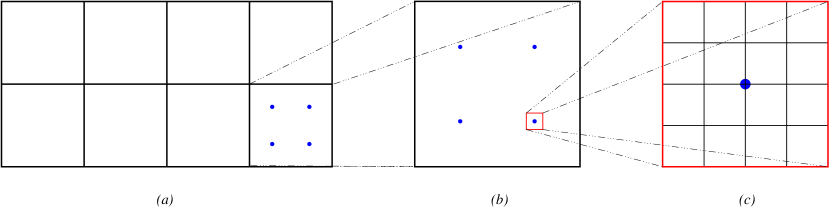
Figure 1: The hierarchy of geometric objects in FEHMM scheme. (a) Domain $\Omega$ and its triangulation ${\mathcal{T}}_{H}$ (b) Macro element $K_{H}$ (c) Sampling domain $K_{\delta,i}$ surrounding a quadrature point $\mathbf{x}_{i}$ and its triangulation ${\mathcal{T}}_{h}$ consisting of micro elements $K_{h}$

Several micro functions will be introduced, which will be used in Section 4. For $j=1,\cdots,d,$ let $\psi^{j}=\psi^{j}(\mathbf{x})\in\widetilde{H}(K_{\delta,i})$ and $\psi^{j}_{h}=\psi^{j}_{h}(\mathbf{x})\in\widetilde{H}_{h}(K_{\delta,i})$ be the solutions of the following micro problems:

(11) $$a^{K_{\delta,i}}(\psi^{j},z)&=-\int_{K_{\delta,i}}\mathbf{A}^{\varepsilon}\mathbf{e}_{j}\cdot\nabla z\kern 0.43057pt\operatorname{d\mathbf{x}}\quad\forall z\in\widetilde{H}(K_{\delta,i}),\\ a^{K_{\delta,i}}_{h}(\psi^{j}_{h},z_{h})=-\sum_{K_{h}\in{\mathcal{T}}_{h}(K_{\delta,i})}\int_{K_{h}}\mathbf{A}^{\varepsilon}\mathbf{e}_{j}\cdot\nabla z_{h}\kern 0.43057pt\operatorname{d\mathbf{x}}\quad\forall z_{h}\in\widetilde{H}_{h}(K_{\delta,i}).$$

Later, $\psi^{j}_{h},j=1,\cdots,d,$ play as basis functions for the solution space of the micro problem (9) on each sampling domain $K_{\delta,i}.$ Instead of $\psi^{j}$ and $\psi^{j}_{h}$, sometimes the following function notations are useful:

(12) $$\varphi^{j}(\mathbf{x}):=\psi^{j}(\mathbf{x})+x_{j}\quad\text{and }\varphi^{j}_{h}(\mathbf{x}):=\psi^{j}_{h}(\mathbf{x})+x_{j}.$$

Notice that the above (11) and (11) are equivalent to

(13) $$a^{K_{\delta,i}}(\varphi^{j},z)&=0\quad\forall z\in\widetilde{H}(K_{\delta,i}),\\ a^{K_{\delta,i}}_{h}(\varphi^{j}_{h},z_{h})=0\quad\forall z_{h}\in\widetilde{H}_{h}(K_{\delta,i}).$$

Remark 3.3.

Indeed, $\psi^{j}$ and $\psi^{j}_{h}$ are nothing but $\psi^{j}=(x_{j})^{m}-x_{j}$ and $\psi^{j}_{h}=(x_{j})^{m}_{h}-x_{j}$, respectively, with the meaning of the superscript ‘$m$’ as same as in (9). Moreover, $\varphi^{j}=(x_{j})^{m}$ and $\varphi^{j}_{h}=(x_{j})^{m}_{h}$.

We also introduce several weak formulations which are used for analysis. A weak formulation of the homogenized problem (2) is given as to find $u^{0}\in V$ such that

$$a^{0}(u^{0},v)=(f,v)\quad\forall v\in V,$$

where

(14) $$a^{0}(v,w)=\int_{\Omega}\mathbf{A}^{0}(\mathbf{x})\nabla v\cdot\nabla w\kern 0.43057pt\operatorname{d\mathbf{x}}\quad\quad\forall v,w\in V.$$

Also, a weak formulation of the homogenized problem (2) with quadrature rule in macro scale, corresponding to (10), can be defined as to find $u^{0}_{H}\in V_{H}$ fulfilling

(15) $$a_{H}^{0}(u^{0}_{H},v_{H})=(f,v_{H})\quad\forall v_{H}\in V_{H},$$

where

(16) $$a_{H}^{0}(v_{H},w_{H})=\sum_{K_{H}\in{\mathcal{T}}_{H}}\sum_{i=1}^{I}\omega_{i}\ \mathbf{A}^{0}(\mathbf{x}_{i})\nabla v_{H}(\mathbf{x}_{i})\cdot\nabla w_{H}(\mathbf{x}_{i})\quad\quad\forall v_{H},w_{H}\in V_{H}.$$

Finally, recalling the bilinear form $\overline{a}_{H}:V_{H}\times V_{H}\rightarrow\mathbb{R}$ defined in (8), define a semi-discrete FEHMM solution $\overline{u}_{H}\in V_{H}$ which satisfy

(17) $$\overline{a}_{H}(\overline{u}_{H},v_{H})=(f,v_{H})\quad\forall v_{H}\in V_{H}.$$

4 Fundamental properties of nonconforming HMM

For our analysis, we mainly follow the framework of [2]. We want to emphasize the changing parts only due to the use of the $P_{1}$–nonconforming quadrilateral finite element space.

4.1 Existence and uniqueness

We begin with the proof of the existence and uniqueness of solutions to (10) and (17).

Lemma 4.1.

Let $v^{m}_{h}$ be the solution of the micro problem (9) with constraint $v_{H}$ on a sampling domain $K_{\delta,i}$. Then

$$|v_{H}|_{1,K_{\delta,i}}\leq{{\left|\kern-1.07639pt\left|\kern-1.07639pt\left|v^{m}_{h}\right|\kern-1.07639pt\right|\kern-1.07639pt\right|}}_{h,K_{\delta,i}}\leq\frac{\Lambda}{\lambda}|v_{H}|_{1,K_{\delta,i}}.$$

Proof 4.2.

Utilizing the fact that $v_{H}$ is linear on $K$ for all $K\in{\mathcal{T}}_{H}$ and (7b), we have

$$0 \leq\sum_{K_{h}\in{\mathcal{T}}_{h}}\int_{K_{h}}\nabla(v^{m}_{h}-v_{H})\cdot\nabla(v^{m}_{h}-v_{H})\kern 0.43057pt\operatorname{d\mathbf{x}}$$

$$=\sum_{K_{h}\in{\mathcal{T}}_{h}}\int_{K_{h}}|\nabla v^{m}_{h}|^{2}-|\nabla v_{H}|^{2}-2\nabla(v^{m}_{h}-v_{H})\cdot\nabla v_{H}\kern 0.43057pt\operatorname{d\mathbf{x}}$$

$$=\Big{[}\sum_{K_{h}\in{\mathcal{T}}_{h}}\int_{K_{h}}|\nabla v^{m}_{h}|^{2}\kern 0.43057pt\operatorname{d\mathbf{x}}-\int_{K_{\delta,i}}|\nabla v_{H}|^{2}\kern 0.43057pt\operatorname{d\mathbf{x}}\Big{]}-2\nabla v_{H}\cdot\sum_{K_{h}\in{\mathcal{T}}_{h}}\int_{\partial K_{h}}{\bm{\nu}}_{K_{h}}(v^{m}_{h}-v_{H})\kern 0.43057pt\operatorname{d}\kern-2.15277pt\bm{\sigma}$$

where ${\bm{\nu}}_{K_{h}}$ denotes the unit outward normal to $K_{h}$. Since $v^{m}_{h}-v_{H}\in\widetilde{H}_{h}(K_{\delta,i})$, the last term in the above equation vanishes. Consequently, we get

$$\int_{K_{\delta,i}}|\nabla v_{H}|^{2}\kern 0.43057pt\operatorname{d\mathbf{x}}\leq\sum_{K_{h}\in{\mathcal{T}}_{h}}\int_{K_{h}}|\nabla v^{m}_{h}|^{2}\kern 0.43057pt\operatorname{d\mathbf{x}}.$$

On the other hand, due to the ellipticity of $\mathbf{A}^{\varepsilon}$, we have

$$0 \leq\sum_{K_{h}\in{\mathcal{T}}_{h}}\int_{K_{h}}\mathbf{A}^{\varepsilon}\nabla(v^{m}_{h}-v_{H})\cdot\nabla(v^{m}_{h}-v_{H})\kern 0.43057pt\operatorname{d\mathbf{x}}$$

$$=\sum_{K_{h}\in{\mathcal{T}}_{h}}\int_{K_{h}}\mathbf{A}^{\varepsilon}\nabla v_{H}\cdot\nabla v_{H}-\mathbf{A}^{\varepsilon}\nabla v^{m}_{h}\cdot\nabla v^{m}_{h}$$

$$\qquad+\mathbf{A}^{\varepsilon}\nabla(v^{m}_{h}-v_{H})\cdot\nabla v^{m}_{h}+\mathbf{A}^{\varepsilon}\nabla v^{m}_{h}\cdot\nabla(v^{m}_{h}-v_{H})\kern 0.43057pt\operatorname{d\mathbf{x}}.$$

Due to the definition of $v^{m}_{h}$ in (9) and symmetry of $\mathbf{A}^{\varepsilon}$, the last two terms vanish. Thus we get

$$\sum_{K_{h}\in{\mathcal{T}}_{h}}\int_{K_{h}}\mathbf{A}^{\varepsilon}\nabla v^{m}_{h}\cdot\nabla v^{m}_{h}\kern 0.43057pt\operatorname{d\mathbf{x}}\leq\int_{K_{\delta,i}}\mathbf{A}^{\varepsilon}\nabla v_{H}\cdot\nabla v_{H}\kern 0.43057pt\operatorname{d\mathbf{x}}.$$

The uniform ellipticity and boundedness of $\mathbf{A}^{\varepsilon}$ imply the desired inequality.

Thanks to the properties of the quadrature formula (6), the bilinear form $a_{H}$ is bounded and coercive in $V_{H}$. Therefore the existence and uniqueness of the solution $u_{H}$ to (10) is guaranteed by the Lax-Milgram Lemma. Thus, we have

Theorem 4.3.

There exists a unique solution $u_{H}$ to the problem (10).

Similarly, the coercivity and boundedness of the bilinear form $\overline{a}_{H}$ can be obtained immediately, and thus one also obtains the existence and uniqueness of the solution $\overline{u}_{H}$ to (17), stated as follows:

Theorem 4.4.

There exists a unique solution $\overline{u}_{H}\in V_{H}$ to Problem (17).

4.2 Recovered homogenized tensors

The recovered homogenized tensors $\overline{\mathbf{A}}^{0}_{K_{\delta,i}}$ and $\mathbf{A}^{0}_{K_{\delta,i}}$ on a sampling domain $K_{\delta,i}$ are defined by

(18a) $$\overline{\mathbf{A}}^{0}_{K_{\delta,i}} =\delta^{-d}\int_{K_{\delta,i}}\mathbf{A}^{\varepsilon}(\mathbf{x})\left(I+\mathbf{J}_{\psi}^{T}\right)\kern 0.43057pt\operatorname{d\mathbf{x}},$$

(18b) $$\mathbf{A}^{0}_{K_{\delta,i}} =\delta^{-d}\sum_{K_{h}\in{\mathcal{T}}_{h}(K_{\delta,i})}\int_{K_{h}}\mathbf{A}^{\varepsilon}(\mathbf{x})\left(I+\mathbf{J}_{\psi_{h}}^{T}\right)\kern 0.43057pt\operatorname{d\mathbf{x}},$$

where $\mathbf{J}_{\psi}$ and $\mathbf{J}_{\psi_{h}}$ are $d\times d$ matrices defined by $\left(J_{\psi}\right)_{jk}=\frac{\partial\psi^{j}}{\partial x_{k}}$ and $\left(J_{\psi_{h}}\right)_{jk}=\frac{\partial\psi^{j}_{h}}{\partial x_{k}},\ 1\leq j,k\leq d,$ respectively. The following propositions show the essential characteristic of two recovered homogenized tensors.

Proposition 4.5.

The following representations hold for $\big{(}\overline{A}^{0}_{K_{\delta,i}}\big{)}_{jk}$ and $\big{(}A^{0}_{K_{\delta,i}}\big{)}_{jk}$:

$$\big{(}\overline{A}^{0}_{K_{\delta,i}}\big{)}_{jk} =\delta^{-d}\int_{K_{\delta,i}}\sum_{\ell=1}^{d}A^{\varepsilon}_{j\ell}\frac{\partial\varphi^{k}}{\partial x_{\ell}}\kern 0.43057pt\operatorname{d\mathbf{x}}=\delta^{-d}\int_{K_{\delta,i}}\mathbf{A}^{\varepsilon}\nabla\varphi^{k}\cdot\nabla x_{j}\kern 0.43057pt\operatorname{d\mathbf{x}}$$

$$=\delta^{-d}\int_{K_{\delta,i}}\mathbf{A}^{\varepsilon}\nabla\varphi^{k}\cdot\nabla\varphi^{j}\kern 0.43057pt\operatorname{d\mathbf{x}},$$

$$\big{(}A^{0}_{K_{\delta,i}}\big{)}_{jk} =\delta^{-d}\sum_{K_{h}\in{\mathcal{T}}_{h}}\int_{K_{h}}\sum_{\ell=1}^{d}A^{\varepsilon}_{j\ell}\frac{\partial\varphi^{k}_{h}}{\partial x_{\ell}}\kern 0.43057pt\operatorname{d\mathbf{x}}=\delta^{-d}\sum_{K_{h}\in{\mathcal{T}}_{h}}\int_{K_{h}}\mathbf{A}^{\varepsilon}\nabla\varphi^{k}_{h}\cdot\nabla x_{j}\kern 0.43057pt\operatorname{d\mathbf{x}}$$

$$=\delta^{-d}\sum_{K_{h}\in{\mathcal{T}}_{h}}\int_{K_{h}}\mathbf{A}^{\varepsilon}\nabla\varphi^{k}_{h}\cdot\nabla\varphi^{j}_{h}\kern 0.43057pt\operatorname{d\mathbf{x}}.$$

Proof 4.6.

The above identities are obtained by the application of the definitions (18) of the recovered homogenized tensors, those (13) of $\varphi^{j}$ and $\varphi_{h}^{j}$, and those of $J_{\psi}$ and $J_{\psi_{h}},$ and Equations (9).

Proposition 4.7.

Let $u^{m}$ and $v^{m}$ be the solutions of the continuous micro problem (9) corresponding to the macro constraints $u_{H}$ and $v_{H}$, respectively, on $K_{\delta,i}$. Then the following holds:

(19) $$\delta^{-d}\int_{K_{\delta,i}}\mathbf{A}^{\varepsilon}\nabla u^{m}\cdot\nabla v^{m}\kern 0.43057pt\operatorname{d\mathbf{x}}=\overline{\mathbf{A}}^{0}_{K_{\delta,i}}\nabla u_{H}\cdot\nabla v_{H}.$$

Similarly, let $u^{m}_{h}$ and $v^{m}_{h}$ be the solutions of the discrete micro problem (9) corresponding to the macro constraints $u_{H}$ and $v_{H}$, respectively, on $K_{\delta,i}$. Then the following holds:

(20) $$\delta^{-d}\sum_{K_{h}\in{\mathcal{T}}_{h}(K_{\delta,i})}\int_{K_{h}}\mathbf{A}^{\varepsilon}\nabla u^{m}_{h}\cdot\nabla v^{m}_{h}\kern 0.43057pt\operatorname{d\mathbf{x}}=\mathbf{A}^{0}_{K_{\delta,i}}\nabla u_{H}\cdot\nabla v_{H}.$$

Proof 4.8.

We will show (20) only, as the proof of (19) follows essentially by the same arguments. Since $u^{m}_{h}$ is the solution of (9), and $v^{m}_{h}-v_{H}\in\widetilde{H}_{h}(K_{\delta,i})$, it holds

(21) $$\delta^{-d}\sum_{K_{h}\in{\mathcal{T}}_{h}}\int_{K_{h}}\mathbf{A}^{\varepsilon}\nabla u^{m}_{h}\cdot\nabla v^{m}_{h}\kern 0.43057pt\operatorname{d\mathbf{x}}=\delta^{-d}\sum_{K_{h}\in{\mathcal{T}}_{h}}\int_{K_{h}}\mathbf{A}^{\varepsilon}\nabla u^{m}_{h}\cdot\nabla v_{H}\kern 0.43057pt\operatorname{d\mathbf{x}}.$$

Since $\nabla u_{H}$ is constant, $u^{m}_{h}$ is represented by a linear combination of the basis functions $\psi^{j}_{h}$ as $u^{m}_{h}=u_{H}+\sum_{j=1}^{d}\psi^{j}_{h}\ \frac{\partial u_{H}}{\partial x_{j}}.$ By plugging this representation into (21), we have

$$\delta^{-d} \sum_{K_{h}\in{\mathcal{T}}_{h}}\int_{K_{h}}\mathbf{A}^{\varepsilon}\Big{(}\nabla u_{H}+\sum_{j=1}^{d}\nabla\psi^{j}_{h}\ \frac{\partial u_{H}}{\partial x_{j}}\Big{)}\cdot\nabla v_{H}\kern 0.43057pt\operatorname{d\mathbf{x}}$$

$$= \delta^{-d}\sum_{K_{h}\in{\mathcal{T}}_{h}}\int_{K_{h}}\mathbf{A}^{\varepsilon}\left(I+J_{\psi_{h}}^{T}\right)\nabla u_{H}\cdot\nabla v_{H}\kern 0.43057pt\operatorname{d\mathbf{x}}=\mathbf{A}^{0}_{K_{\delta,i}}\nabla u_{H}\cdot\nabla v_{H}.$$

This completes the proof.

Remark 4.9.

Proposition 4.7 implies that $\mathbf{A}^{0}_{K_{\delta,i}}$ indeed plays a role as the homogenized tensor on each sampling domain $K_{\delta,i}$ numerically.

4.3 The case of periodic coupling

In this section, main ingredients of error analysis are provided under periodic assumptions. Recall the definitions of $\psi^{j}$ and $\varphi^{j}$ in (11) and (12). The following two assumptions will be taken into consideration in this section.

Assumption 4.10 (Periodic coupling).

1. $\mathbf{A}^{\varepsilon}(\mathbf{x}):=\mathbf{A}(\mathbf{x},\frac{\mathbf{x}}{\varepsilon})$ where $\mathbf{A}(\mathbf{x},\cdot)$ is $Y$-periodic with $Y=[0,1]^{d}$ and $\mathbf{A}(\mathbf{x},\cdot)\in\mathbf{W}^{1,\infty}(Y)$.

2. On each sampling domain $K_{\delta,i}$, the solution of the micro problem (11) with periodic coupling (7a) has regularity $\psi^{j}\in H^{2}(K_{\delta,i})$ and $\mathbf{A}^{\varepsilon}\nabla\varphi^{j}\in[H^{1}(K_{\delta,i})]^{d}$.

First, we note the following lemmas. The proofs follow the main framework and are omitted.

Lemma 4.11.

Under Assumption 4.10, $\nabla\cdot\left(\mathbf{A}^{\varepsilon}\nabla\varphi^{j}\right)=0$ on $K_{\delta,i}$ a.e.

Lemma 4.12.

Under Assumption 4.10, it holds

(22) $$|\mathbf{A}^{\varepsilon}\nabla\varphi^{j}|_{1,K_{\delta,i}}\leq C\delta^{\frac{d}{2}}\varepsilon^{-1}.$$

The following proposition is a discretization error estimation of the micro basis function $\psi^{j}$.

Proposition 4.13.

Under Assumption 4.10, it holds

(23) $${{\left|\kern-1.07639pt\left|\kern-1.07639pt\left|\psi^{j}-\psi^{j}_{h}\right|\kern-1.07639pt\right|\kern-1.07639pt\right|}}_{h,K_{\delta,i}} \leq Ch\delta^{\frac{d}{2}}\varepsilon^{-1}.$$

Proof 4.14.

The Second Strang Lemma [48, 9] for the micro problems (11) and (11) implies that

$${{\left|\kern-1.07639pt\left|\kern-1.07639pt\left|\psi^{j}-\psi^{j}_{h}\right|\kern-1.07639pt\right|\kern-1.07639pt\right|}}_{h,K_{\delta,i}} \leq C\Big{(}\inf_{v_{h}\in\widetilde{H}_{h}(K_{\delta,i})}{{\left|\kern-1.07639pt\left|\kern-1.07639pt\left|\psi^{j}-v_{h}\right|\kern-1.07639pt\right|\kern-1.07639pt\right|}}_{h,K_{\delta,i}}$$

$$\qquad+\sup_{w_{h}\in\widetilde{H}_{h}(K_{\delta,i})}\frac{\big{|}a^{K_{\delta,i}}_{h}(\psi^{j},w_{h})-a^{K_{\delta,i}}_{h}(\psi^{j}_{h},w_{h})\big{|}}{{{\left|\kern-1.07639pt\left|\kern-1.07639pt\left|w_{h}\right|\kern-1.07639pt\right|\kern-1.07639pt\right|}}_{h,K_{\delta,i}}}\Big{)}.$$

The first term represents the best approximation error of $\psi^{j},$ which is of $\mathcal{O}(h)$ due to the standard approximation property of nonconforming element spaces. The second term, so-called the consistency error, measures nonconformity of the finite element space. Denoting by $L(w_{h})$ the numerator of the second term, from the definitions (11) and (12) of $\psi^{j}_{h}$ and $\varphi^{j}$ one sees that

$$\left|L(w_{h})\right| =\Big{|}\sum_{K_{h}\in{\mathcal{T}}_{h}}\int_{K_{h}}\mathbf{A}^{\varepsilon}\nabla\psi^{j}\cdot\nabla w_{h}\kern 0.43057pt\operatorname{d\mathbf{x}}+\sum_{K_{h}\in{\mathcal{T}}_{h}}\int_{K_{h}}\mathbf{A}^{\varepsilon}\mathbf{e}_{j}\cdot\nabla w_{h}\kern 0.43057pt\operatorname{d\mathbf{x}}\Big{|}$$

$$=\Big{|}\sum_{K_{h}\in{\mathcal{T}}_{h}}\int_{K_{h}}\mathbf{A}^{\varepsilon}\nabla\varphi^{j}\cdot\nabla w_{h}\kern 0.43057pt\operatorname{d\mathbf{x}}\Big{|}$$

$$=\Big{|}\sum_{K_{h}\in{\mathcal{T}}_{h}}\int_{\partial K_{h}}{\bm{\nu}}_{K_{h}}\cdot\left(\mathbf{A}^{\varepsilon}\nabla\varphi^{j}\right)w_{h}\kern 0.43057pt\operatorname{d}\kern-2.15277pt\bm{\sigma}-\sum_{K_{h}\in{\mathcal{T}}_{h}}\int_{K_{h}}\nabla\cdot\left(\mathbf{A}^{\varepsilon}\nabla\varphi^{j}\right)w_{h}\kern 0.43057pt\operatorname{d\mathbf{x}}\Big{|}.$$

Due to Lemma 4.11, the above equation is bounded by only the first term such that

$$\Big{|}\sum_{K_{h}\in{\mathcal{T}}_{h}}\int_{\partial K_{h}}{\bm{\nu}}_{K_{h}}\cdot\mathbf{A}^{\varepsilon}\nabla\varphi^{j}w_{h}\kern 0.43057pt\operatorname{d}\kern-2.15277pt\bm{\sigma}\Big{|} =\Big{|}\sum_{K_{h}\in{\mathcal{T}}_{h}}\sum_{\tau\in\mathcal{F}(K_{h})}\int_{\tau}{\bm{\nu}}_{K_{h}}\cdot\mathbf{A}^{\varepsilon}\nabla\varphi^{j}w_{h}\kern 0.43057pt\operatorname{d}\kern-2.15277pt\bm{\sigma}\Big{|}$$

$$\leq\sum_{\tau\in\mathcal{F}_{h}}\Big{|}\int_{\tau}{\bm{\nu}}_{\tau}\cdot\mathbf{A}^{\varepsilon}\nabla\varphi^{j}[w_{h}]_{\tau}\kern 0.43057pt\operatorname{d}\kern-2.15277pt\bm{\sigma}\Big{|}.$$

Thanks to the regularity in Assumption 4.10, the Bramble–Hilbert lemma, and the trace theorem, one sees that

$$\int_{\tau}{\bm{\nu}}_{\tau}\cdot\mathbf{A}^{\varepsilon}\nabla\varphi^{j}[w_{h}]_{\tau}\kern 0.43057pt\operatorname{d}\kern-2.15277pt\bm{\sigma} =\int_{\tau}{\bm{\nu}}_{\tau}\cdot\mathbf{A}^{\varepsilon}\nabla\varphi^{j}\big{[}w_{h}-\mathop{\ooalign{$\int$\cr$-$}}_{\tau}w_{h}\big{]}_{\tau}\kern 0.43057pt\operatorname{d}\kern-2.15277pt\bm{\sigma}$$

$$=\int_{\tau}{\bm{\nu}}_{\tau}\cdot\big{[}\mathbf{A}^{\varepsilon}\nabla\varphi^{j}-\mathop{\ooalign{$\int$\cr$-$}}_{\tau}\big{(}\mathbf{A}^{\varepsilon}\nabla\varphi^{j}\big{)}\big{]}\big{[}w_{h}-\mathop{\ooalign{$\int$\cr$-$}}_{\tau}w_{h}\big{]}_{\tau}\kern 0.43057pt\operatorname{d}\kern-2.15277pt\bm{\sigma}$$

$$\leq\big{[}\int_{\tau}\big{|}\mathbf{A}^{\varepsilon}\nabla\varphi^{j}-\mathop{\ooalign{$\int$\cr$-$}}_{\tau}\left(\mathbf{A}^{\varepsilon}\nabla\varphi^{j}\right)\big{|}^{2}\kern 0.43057pt\operatorname{d}\kern-2.15277pt\bm{\sigma}\big{]}^{\frac{1}{2}}\big{[}\int_{\tau}\big{|}w_{h}-\mathop{\ooalign{$\int$\cr$-$}}_{\tau}w_{h}\big{|}^{2}\kern 0.43057pt\operatorname{d}\kern-2.15277pt\bm{\sigma}\big{]}^{\frac{1}{2}}$$

$$\leq Ch^{\frac{1}{2}}\left|\mathbf{A}^{\varepsilon}\nabla\varphi^{j}\right|_{1/2,\tau}h^{\frac{1}{2}}\left|w_{h}\right|_{1/2,\tau}$$

$$\leq Ch\left|\mathbf{A}^{\varepsilon}\nabla\varphi^{j}\right|_{1,K_{h}}\left|w_{h}\right|_{1,K_{h}},\quad\tau\in\mathcal{F}(K_{h}).$$

Consequently, we have

$$\left|L(w_{h})\right| \leq C\sum_{K_{h}\in{\mathcal{T}}_{h}}h|\mathbf{A}^{\varepsilon}\nabla\varphi^{j}|_{1,K_{h}}|w_{h}|_{1,K_{h}}$$

$$\leq Ch\big{[}\sum_{K_{h}\in{\mathcal{T}}_{h}}|\mathbf{A}^{\varepsilon}\nabla\varphi^{j}|_{1,K_{h}}^{2}\big{]}^{1/2}\big{[}\sum_{K_{h}\in{\mathcal{T}}_{h}}|w_{h}|^{2}_{1,K_{h}}\big{]}^{1/2}$$

$$=Ch|\mathbf{A}^{\varepsilon}\nabla\varphi^{j}|_{1,K_{\delta,i}}{{\left|\kern-1.07639pt\left|\kern-1.07639pt\left|w_{h}\right|\kern-1.07639pt\right|\kern-1.07639pt\right|}}_{h,K_{\delta,i}}.$$

Finally, Lemma 4.12 and the regularity result imply the desired error estimate:

$${{\left|\kern-1.07639pt\left|\kern-1.07639pt\left|\psi^{j}-\psi^{j}_{h}\right|\kern-1.07639pt\right|\kern-1.07639pt\right|}}_{h,K_{\delta,i}} \leq Ch\left(|\psi^{j}|_{2,K_{\delta,i}}+|\mathbf{A}^{\varepsilon}\nabla\varphi^{j}|_{1,h,K_{\delta,i}}\right)\leq Ch\delta^{\frac{d}{2}}\varepsilon^{-1}.$$

The following proposition shows difference between the recovered homogenized tensors.

Proposition 4.15.

Under Assumption 4.10, the following holds:

(24) $$\sup_{K_{\delta,i}}\|\overline{\mathbf{A}}^{0}_{K_{\delta,i}}-\mathbf{A}^{0}_{K_{\delta,i}}\|_{2}\leq C\Big{(}\frac{h}{\varepsilon}\Big{)}^{2},$$

where $\|\cdot\|_{2}$ denotes the matrix 2–norm.

Proof 4.16.

Invoking Proposition 4.5, we have

$$\big{|}\big{(}\mathbf{A}^{0}_{K_{\delta,i}}\big{)}_{jk}-\big{(}\overline{\mathbf{A}}^{0}_{K_{\delta,i}}\big{)}_{jk}\big{|}$$

$$=\Big{|}\delta^{-d}\sum_{K_{h}\in{\mathcal{T}}_{h}}\int_{K_{h}}\mathbf{A}^{\varepsilon}\nabla\varphi^{k}_{h}\cdot\nabla\varphi^{j}_{h}-\mathbf{A}^{\varepsilon}\nabla\varphi^{k}\cdot\nabla\varphi^{j}\kern 0.43057pt\operatorname{d\mathbf{x}}\Big{|}$$

$$=\Big{|}\delta^{-d}\sum_{K_{h}\in{\mathcal{T}}_{h}}\int_{K_{h}}\mathbf{A}^{\varepsilon}\nabla\big{(}\varphi^{k}_{h}-\varphi^{k}\big{)}\cdot\nabla\big{(}\varphi^{j}_{h}-\varphi^{j}\big{)}$$

$$\qquad\qquad\qquad\qquad\qquad+\mathbf{A}^{\varepsilon}\nabla\varphi^{k}\cdot\nabla\big{(}\varphi^{j}_{h}-\varphi^{j}\big{)}+\mathbf{A}^{\varepsilon}\nabla\big{(}\varphi^{k}_{h}-\varphi^{k}\big{)}\cdot\nabla\varphi^{j}\kern 0.43057pt\operatorname{d\mathbf{x}}\Big{|}$$

$$\leq\delta^{-d}\Big{|}\sum_{K_{h}\in{\mathcal{T}}_{h}}\int_{K_{h}}\mathbf{A}^{\varepsilon}\nabla\big{(}\varphi^{k}_{h}-\varphi^{k}\big{)}\cdot\nabla\big{(}\varphi^{j}_{h}-\varphi^{j}\big{)}\kern 0.43057pt\operatorname{d\mathbf{x}}\Big{|}$$

$$\quad+\delta^{-d}\Big{|}\sum_{K_{h}\in{\mathcal{T}}_{h}}-\int_{K_{h}}\nabla\cdot\big{(}\mathbf{A}^{\varepsilon}\nabla\varphi^{k}\big{)}\big{(}\varphi^{j}_{h}-\varphi^{j}\big{)}\kern 0.43057pt\operatorname{d\mathbf{x}}+\int_{\partial K_{h}}{\bm{\nu}}_{K_{h}}\cdot\mathbf{A}^{\varepsilon}\nabla\varphi^{k}\big{(}\varphi^{j}_{h}-\varphi^{j}\big{)}\kern 0.43057pt\operatorname{d}\kern-2.15277pt\bm{\sigma}\Big{|}$$

$$\quad+\delta^{-d}\Big{|}\sum_{K_{h}\in{\mathcal{T}}_{h}}-\int_{K_{h}}\nabla\cdot\big{(}\mathbf{A}^{\varepsilon}\nabla\varphi^{j}\big{)}\big{(}\varphi^{k}_{h}-\varphi^{k}\big{)}\kern 0.43057pt\operatorname{d\mathbf{x}}+\int_{\partial K_{h}}{\bm{\nu}}_{K_{h}}\cdot\mathbf{A}^{\varepsilon}\nabla\varphi^{j}\big{(}\varphi^{k}_{h}-\varphi^{k}\big{)}\kern 0.43057pt\operatorname{d}\kern-2.15277pt\bm{\sigma}\Big{|}.$$

The last inequality is due to an integration by parts and the symmetry of $\mathbf{A}^{\varepsilon}$. By Lemmas 4.11 and  4.12, and Proposition 4.13 with proper modifications, the terms in the last inequality is further bounded by

$$\leq\frac{\Lambda}{\delta^{d}}{{\left|\kern-1.07639pt\left|\kern-1.07639pt\left|\varphi^{k}_{h}-\varphi^{k}\right|\kern-1.07639pt\right|\kern-1.07639pt\right|}}_{h,K_{\delta,i}}{{\left|\kern-1.07639pt\left|\kern-1.07639pt\left|\varphi^{j}_{h}-\varphi^{j}\right|\kern-1.07639pt\right|\kern-1.07639pt\right|}}_{h,K_{\delta,i}}$$

$$\qquad+\delta^{-d}\Big{|}\sum_{K_{h}\in{\mathcal{T}}_{h}}\int_{\partial K_{h}}{\bm{\nu}}_{K_{h}}\cdot\mathbf{A}^{\varepsilon}\nabla\varphi^{k}\big{(}\varphi^{j}_{h}-\varphi^{j}\big{)}\kern 0.43057pt\operatorname{d}\kern-2.15277pt\bm{\sigma}\Big{|}$$

$$\qquad+\delta^{-d}\Big{|}\sum_{K_{h}\in{\mathcal{T}}_{h}}\int_{\partial K_{h}}{\bm{\nu}}_{K_{h}}\cdot\mathbf{A}^{\varepsilon}\nabla\varphi^{j}\big{(}\varphi^{k}_{h}-\varphi^{k}\big{)}\kern 0.43057pt\operatorname{d}\kern-2.15277pt\bm{\sigma}\Big{|}$$

$$\leq\frac{\Lambda}{\delta^{d}}{{\left|\kern-1.07639pt\left|\kern-1.07639pt\left|\varphi^{k}_{h}-\varphi^{k}\right|\kern-1.07639pt\right|\kern-1.07639pt\right|}}_{h,K_{\delta,i}}{{\left|\kern-1.07639pt\left|\kern-1.07639pt\left|\varphi^{j}_{h}-\varphi^{j}\right|\kern-1.07639pt\right|\kern-1.07639pt\right|}}_{h,K_{\delta,i}}$$

$$\qquad+\delta^{-d}h|\mathbf{A}^{\varepsilon}\nabla\varphi^{k}|_{1,K_{\delta,i}}{{\left|\kern-1.07639pt\left|\kern-1.07639pt\left|\varphi^{j}_{h}-\varphi^{j}\right|\kern-1.07639pt\right|\kern-1.07639pt\right|}}_{h,K_{\delta,i}}+\delta^{-d}h|\mathbf{A}^{\varepsilon}\nabla\varphi^{j}|_{1,K_{\delta,i}}{{\left|\kern-1.07639pt\left|\kern-1.07639pt\left|\varphi^{k}_{h}-\varphi^{k}\right|\kern-1.07639pt\right|\kern-1.07639pt\right|}}_{h,K_{\delta,i}}$$

$$\leq C\Big{(}\frac{h}{\varepsilon}\Big{)}^{2}.$$

This completes the proof.

4.4 The case of Dirichlet coupling

In this subsection we consider the following assumptions and the Dirichlet coupling condition for micro problems.

Assumption 4.17 (Dirichlet coupling).

1. $\mathbf{A}^{\varepsilon}(\mathbf{x})\in\widetilde{H}^{1,\infty}(K_{H})$ with $|A^{\varepsilon}_{jk}|_{0,\infty,K_{H}}\leq C$ and $|\nabla A^{\varepsilon}_{jk}|_{0,\infty,K_{H}}\leq C/\varepsilon$ for all $K_{H}\in{\mathcal{T}}_{H}$.

2. On each sampling domain $K_{\delta,i}$, the solution of the micro problem (11) with Dirichlet coupling (7a) has regularity $\psi^{j}\in H^{2}(K_{\delta,i})$ and $\mathbf{A}^{\varepsilon}\nabla\varphi^{j}\in[H^{1}(K_{\delta,i})]^{2}$.

The same arguments as in the case of periodic coupling in Section 4.3 leads to the corresponding results to Propositions 4.13 and  4.15 hold under Assumption 4.17. Omitting the details of proof, we state the results as follows:

Proposition 4.18.

Under Assumption 4.17, it holds

(25) $${{\left|\kern-1.07639pt\left|\kern-1.07639pt\left|\psi^{j}-\psi^{j}_{h}\right|\kern-1.07639pt\right|\kern-1.07639pt\right|}}_{h,K_{\delta,i}} \leq Ch\delta^{\frac{d}{2}}\varepsilon^{-1}.$$

Proposition 4.19.

Under Assumption 4.17, the following holds:

(26) $$\sup_{K_{\delta,i}}\|\overline{\mathbf{A}}^{0}_{K_{\delta,i}}-\mathbf{A}^{0}_{K_{\delta,i}}\|_{2}\leq C\Big{(}\frac{h}{\varepsilon}\Big{)}^{2}.$$

4.5 A priori error estimate

The description below is following the analysis framework from [2], but adopting the finite element specific results above. We do not repeat the details of proof in this section.

4.5.1 The macro error

Under sufficient regularity of $u^{0}$, for instance $H^{2}(\Omega)$, the standard analysis for nonconforming finite elements [43] yields

(27) $${{\left|\kern-1.07639pt\left|\kern-1.07639pt\left|u^{0}-u^{0}_{H}\right|\kern-1.07639pt\right|\kern-1.07639pt\right|}}_{H}\leq CH\|u^{0}\|_{2}.$$

4.5.2 The modeling error

Since $\overline{u}_{H},u^{0}_{H}\in V_{H}$, using the uniform ellipticity of $\overline{a}_{H}$ (17), and (15), we have

$${{\left|\kern-1.07639pt\left|\kern-1.07639pt\left|u^{0}_{H}-\overline{u}_{H}\right|\kern-1.07639pt\right|\kern-1.07639pt\right|}}_{H}^{2} \leq\overline{a}_{H}(u^{0}_{H}-\overline{u}_{H},u^{0}_{H}-\overline{u}_{H})$$

$$=\overline{a}_{H}(u^{0}_{H},u^{0}_{H}-\overline{u}_{H})-a_{H}^{0}(u^{0}_{H},u^{0}_{H}-\overline{u}_{H}).$$

We deduce the following Strang-type inequality:

(28) $${{\left|\kern-1.07639pt\left|\kern-1.07639pt\left|u^{0}_{H}-\overline{u}_{H}\right|\kern-1.07639pt\right|\kern-1.07639pt\right|}}_{H} \leq\sup_{w_{H}\in V_{H}}\frac{\left|\overline{a}_{H}(u^{0}_{H},w_{H})-a_{H}^{0}(u^{0}_{H},w_{H})\right|}{{{\left|\kern-1.07639pt\left|\kern-1.07639pt\left|w_{H}\right|\kern-1.07639pt\right|\kern-1.07639pt\right|}}_{H}}.$$

Recalling (8) and (16), and using Proposition 4.7, we can bound the numerator as follows:

$$\left|\overline{a}_{H}(u^{0}_{H},w_{H})-a_{H}^{0}(u^{0}_{H},w_{H})\right|$$

$$=\Big{|}\sum_{K_{H}\in{\mathcal{T}}_{H}}\sum_{i=1}^{I}\omega_{i}\ \overline{\mathbf{A}}^{0}_{K_{\delta,i}}\nabla{u^{0}_{H}}\cdot\nabla{w_{H}}-\sum_{K_{H}\in{\mathcal{T}}_{H}}\sum_{i=1}^{I}\omega_{i}\ \mathbf{A}^{0}(\mathbf{x}_{i})\nabla u^{0}_{H}(\mathbf{x}_{i})\cdot\nabla w_{H}(\mathbf{x}_{i})\Big{|}$$

$$\leq\sum_{K_{H}\in{\mathcal{T}}_{H}}\sum_{i=1}^{I}\omega_{i}\Big{|}\big{(}\overline{\mathbf{A}}^{0}_{K_{\delta,i}}-\mathbf{A}^{0}(\mathbf{x}_{i})\big{)}\nabla{u^{0}_{H}}\cdot\nabla{w_{H}}\Big{|}$$

$$\leq\sup_{K_{\delta,i}}\|\overline{\mathbf{A}}^{0}_{K_{\delta,i}}-\mathbf{A}^{0}(\mathbf{x}_{i})\|_{2}\ {{\left|\kern-1.07639pt\left|\kern-1.07639pt\left|u^{0}_{H}\right|\kern-1.07639pt\right|\kern-1.07639pt\right|}}_{H}\ {{\left|\kern-1.07639pt\left|\kern-1.07639pt\left|w_{H}\right|\kern-1.07639pt\right|\kern-1.07639pt\right|}}_{H}.$$

Thus, we have

(29) $${{\left|\kern-1.07639pt\left|\kern-1.07639pt\left|u^{0}_{H}-\overline{u}_{H}\right|\kern-1.07639pt\right|\kern-1.07639pt\right|}}_{H} \leq C\sup_{K_{\delta,i}}\|\overline{\mathbf{A}}^{0}_{K_{\delta,i}}-\mathbf{A}^{0}(\mathbf{x}_{i})\|_{2}\,{{\left|\kern-1.07639pt\left|\kern-1.07639pt\left|u^{0}_{H}\right|\kern-1.07639pt\right|\kern-1.07639pt\right|}}_{H}.$$

As mentioned in [2], the following result is obtained in [20]: If we assume the local periodicity of $\mathbf{A}^{\varepsilon}$, for instance under Assumption 4.10, then

(30) $$\sup_{K_{\delta,i}}\|\mathbf{A}^{0}-\overline{\mathbf{A}}^{0}_{K_{\delta,i}}\|_{2}\leq\begin{cases}C\varepsilon&\text{if periodic coupling with }\delta/\varepsilon\in\mathbb{N}\text{ is used for }\eqref{eq:micro-problem},\\ C\left(\frac{\varepsilon}{\delta}+\delta\right)&\text{if Dirichlet coupling or }\delta/\varepsilon\not\in\mathbb{N}\text{ is used}.\end{cases}$$

4.5.3 The micro error

Due to the uniform ellipticity of $a_{H}$, we have

$${{\left|\kern-1.07639pt\left|\kern-1.07639pt\left|\overline{u}_{H}-u_{H}\right|\kern-1.07639pt\right|\kern-1.07639pt\right|}}_{H}^{2} \leq a_{H}(\overline{u}_{H}-u_{H},\overline{u}_{H}-u_{H})$$

$$=a_{H}(\overline{u}_{H},\overline{u}_{H}-u_{H})-\overline{a}_{H}(\overline{u}_{H},\overline{u}_{H}-u_{H}).$$

Therefore it holds

(31) $${{\left|\kern-1.07639pt\left|\kern-1.07639pt\left|\overline{u}_{H}-u_{H}\right|\kern-1.07639pt\right|\kern-1.07639pt\right|}}_{H} \leq\sup_{w_{H}\in V_{H}}\frac{\left|a_{H}(\overline{u}_{H},w_{H})-\overline{a}_{H}(\overline{u}_{H},w_{H})\right|}{{{\left|\kern-1.07639pt\left|\kern-1.07639pt\left|w_{H}\right|\kern-1.07639pt\right|\kern-1.07639pt\right|}}_{H}}.$$

Again, recalling (8) and (16), we see that an application of Propositions 4.7 and  4.15 to the numerator gives the following bound:

$$\left|a_{H}(\overline{u}_{H},w_{H})-\overline{a}_{H}(\overline{u}_{H},w_{H})\right|$$

$$=\Big{|}\sum_{K_{H}\in{\mathcal{T}}_{H}}\sum_{i=1}^{I}\omega_{i}\ \mathbf{A}^{0}_{K_{\delta,i}}\nabla{\overline{u}_{H}}\cdot\nabla{w_{H}}-\sum_{K_{H}\in{\mathcal{T}}_{H}}\sum_{i=1}^{I}\omega_{i}\ \overline{\mathbf{A}}^{0}_{K_{\delta,i}}\nabla{\overline{u}_{H}}\cdot\nabla{w_{H}}\Big{|}$$

$$\leq\sum_{K_{H}\in{\mathcal{T}}_{H}}\sum_{i=1}^{I}\omega_{i}\Big{|}\big{(}\mathbf{A}^{0}_{K_{\delta,i}}-\overline{\mathbf{A}}^{0}_{K_{\delta,i}}\big{)}\nabla{\overline{u}_{H}}\cdot\nabla{w_{H}}\Big{|}$$

$$\leq\sup_{K_{\delta,i}}\|\mathbf{A}^{0}_{K_{\delta,i}}-\overline{\mathbf{A}}^{0}_{K_{\delta,i}}\|_{2}\ {{\left|\kern-1.07639pt\left|\kern-1.07639pt\left|\overline{u}_{H}\right|\kern-1.07639pt\right|\kern-1.07639pt\right|}}_{H}\ {{\left|\kern-1.07639pt\left|\kern-1.07639pt\left|w_{H}\right|\kern-1.07639pt\right|\kern-1.07639pt\right|}}_{H}\leq C\Big{(}\frac{h}{\varepsilon}\Big{)}^{2}{{\left|\kern-1.07639pt\left|\kern-1.07639pt\left|\overline{u}_{H}\right|\kern-1.07639pt\right|\kern-1.07639pt\right|}}_{H}\ {{\left|\kern-1.07639pt\left|\kern-1.07639pt\left|w_{H}\right|\kern-1.07639pt\right|\kern-1.07639pt\right|}}_{H},$$

and we have

(32) $${{\left|\kern-1.07639pt\left|\kern-1.07639pt\left|\overline{u}_{H}-u_{H}\right|\kern-1.07639pt\right|\kern-1.07639pt\right|}}_{H} \leq C\Big{(}\frac{h}{\varepsilon}\Big{)}^{2}{{\left|\kern-1.07639pt\left|\kern-1.07639pt\left|\overline{u}_{H}\right|\kern-1.07639pt\right|\kern-1.07639pt\right|}}_{H}.$$

4.5.4 Main theorem for error estimates

The usual Aubin-Nitsche duality argument provides $L^{2}$-norm error estimates, see, for instance, [20]. The derivation is standard, omitted here, but we list the estimates:

Theorem 4.20.

Let $u^{0}$ and $u_{H}$ be the solutions of (2) and (10). Then, the followings hold under various assumptions:

1. Under Assumption 4.10, if periodic coupling with $\delta/\varepsilon\in\mathbb{N}$ is used, then

   (33a) $${{\left|\kern-1.07639pt\left|\kern-1.07639pt\left|u^{0}-u_{H}\right|\kern-1.07639pt\right|\kern-1.07639pt\right|}}_{H}\leq C\Big{(}H+\varepsilon+\big{(}\frac{h}{\varepsilon}\big{)}^{2}\Big{)},$$

   (33b) $$\|u^{0}-u_{H}\|_{0}\leq C\Big{(}H^{2}+\varepsilon+\big{(}\frac{h}{\varepsilon}\big{)}^{2}\Big{)};$$

2. Under Assumption 4.10, if periodic coupling with $\delta/\varepsilon\not\in\mathbb{N}$ is used, then

   (34a) $${{\left|\kern-1.07639pt\left|\kern-1.07639pt\left|u^{0}-u_{H}\right|\kern-1.07639pt\right|\kern-1.07639pt\right|}}_{H}\leq C\Big{(}H+\big{(}\frac{\varepsilon}{\delta}+\delta\big{)}+\big{(}\frac{h}{\varepsilon}\big{)}^{2}\Big{)},$$

   (34b) $$\|u^{0}-u_{H}\|_{0}\leq C\Big{(}H^{2}+\big{(}\frac{\varepsilon}{\delta}+\delta\big{)}+\big{(}\frac{h}{\varepsilon}\big{)}^{2}\Big{)};$$

3. Under Assumption 4.10 and Assumption 4.17, if Dirichlet coupling is used, then

   (35a) $${{\left|\kern-1.07639pt\left|\kern-1.07639pt\left|u^{0}-u_{H}\right|\kern-1.07639pt\right|\kern-1.07639pt\right|}}_{H}\leq C\Big{(}H+\big{(}\frac{\varepsilon}{\delta}+\delta\big{)}+\big{(}\frac{h}{\varepsilon}\big{)}^{2}\Big{)},$$

   (35b) $$\|u^{0}-u_{H}\|_{0}\leq C\Big{(}H^{2}+\big{(}\frac{\varepsilon}{\delta}+\delta\big{)}+\big{(}\frac{h}{\varepsilon}\big{)}^{2}\Big{)};$$

4. Under Assumption 4.17, if Dirichlet coupling is used, then

   (36a) $${{\left|\kern-1.07639pt\left|\kern-1.07639pt\left|u^{0}-u_{H}\right|\kern-1.07639pt\right|\kern-1.07639pt\right|}}_{H}\leq C\Big{(}H+\sup_{K_{\delta,i}}\|\overline{\mathbf{A}}^{0}_{K_{\delta,i}}-\mathbf{A}^{0}(\mathbf{x}_{i})\|_{2}+\big{(}\frac{h}{\varepsilon}\big{)}^{2}\Big{)},$$

   (36b) $$\|u^{0}-u_{H}\|_{0}\leq C\Big{(}H^{2}+\sup_{K_{\delta,i}}\|\overline{\mathbf{A}}^{0}_{K_{\delta,i}}-\mathbf{A}^{0}(\mathbf{x}_{i})\|_{2}+\big{(}\frac{h}{\varepsilon}\big{)}^{2}\Big{)}.$$

5 Numerical results

In this section, we have numerical tests for homogeneous finite element scheme. We need to pay attention to solving the micro problems since it may treats problems with periodic boundary condition. If the periodic coupling condition is adopted for the micro problems, the corresponding algebraic system of equations for each micro problem must be constructed in order to fulfill two important properties, namely, the periodicity and the zero-integral properties. Technically, these properties can be enforced either in the discrete function space or in the formulation for the problem.

In [4] these two properties are imposed at the level of the problem formulation, by using a Lagrange multiplier and a constraint matrix. This approach is quite simple to implement, but the resulting linear systems are saddle point problems. It requires an additional consideration to apply an efficient iterative method for such indefinite problems, and thus a direct method is often employed as in [4].

Alternative approaches for the $P_{1}$–nonconforming quadrilateral finite element [43] are proposed in [50]. To handle elliptic problems with periodic boundary condition, they introduce a subspace of the lowest order nonconforming quadrilateral finite element which is required to have the periodicity and iterative-based numerical schemes which deals the zero–integral. Those approaches assemble semi-definite matrix equations without additional columns for constraints. The semi-definiteness is advantageous for the numerical schemes since it derives faster convergence. Theoretical results of the numerical schemes for the semi-definite matrix equations show a priori error estimate of the numerical solutions.

In our numerical examples, we employ one of alternative approaches from [50] to solve micro problems. We take $\mathfrak{E}^{\flat}$, a linearly independent basis for $V^{P_{1}}_{h,\#}$, as the trial and test function space and assemble the corresponding linear system without the zero–integral condition. The corresponding stiffness matrix is a symmetric positive semi-definite system whose rank deficiency is 1. For details about the numerical implementation, see Section 5.2 in [50]. We will investigate efficiency of the alternative approach for micro problems in Section 5.1.1. It should be mentioned that we use the 2-point Gauss-Legendre quadrature formula for each coordinate in all numerical examples.

5.1 Periodic diagonal example

The first example is a multiscale elliptic problem (1) in $\Omega=(0,1)^{2}$ whose coefficient is anisotropically periodic in micro scale:

$$\mathbf{A}^{\varepsilon}({\mathbf{x}})=\begin{pmatrix}\sqrt{2}+\sin(2\pi{x_{1}}/{\varepsilon})&0\\ 0&\sqrt{2}+\sin(2\pi{x_{2}}/{\varepsilon})\end{pmatrix},\quad\varepsilon=10^{-3}.$$

By the homogenization theory, it can be easily shown that the associated homogenized tensor $\mathbf{A}^{0}$ is equal to $I$, the identity tensor. $f(\mathbf{x})$ is set to satisfy that the associated homogenized elliptic problem has the exact solution $u^{0}({\mathbf{x}})=\sin(\pi x_{1})\sin(\pi x_{2})$. For the sake of simplicity we use the macro and the micro mesh consisting of uniform squares. The size parameter $\delta$ of each sampling domain is set to be same as $\varepsilon$. We use periodic coupling for micro problems.

Figure 2 shows error in energy norm, and in $L^{2}$-norm, and the difference between two observable homogenized tensors $\mathbf{A}^{0}$ and $\mathbf{A}^{0}_{K_{\delta,i}}$ in the Frobenius norm. Note that the matrix $2-$norm for a finite dimensional matrix is equivalent to the Frobenius norm. The theoretical error estimates (33) depend on $H$ as well as $h$. We can observe that the error is decreasing as $H$ is decreasing, but there is a critical $H$ value where the error does not decrease anymore for fixed $h$, as particularly in $L^{2}$-norm. Furthermore, in order to observe convergence rate as in (33) we have to consider simultaneous reduction of $H$ and $h$ in different orders, since the theorem shows the dependency on $H$ and $h$ with their own convergence orders. For instance, simultaneous reduction of $H$ in the second-order and $h$ in the first-order gives convergence order of 2 in energy norm, as observed in the table. The error in $L^{2}$-norm is similar. The numerical results confirm (33) in Theorem 4.20, the main convergence result for periodic cases.

$H$	$h/\varepsilon$=1/4	1/8	1/16	1/32	1/64
	${{\left|\kern-0.8611pt\left|\kern-0.8611pt\left|u^{0}-u_{H}\right|\kern-0.8611pt\right|\kern-0.8611pt\right|}}_{H}$
1/2	1.33E-00	1.35E-00	1.36E-00	1.36E-00	1.36E-00
1/4	6.98E-01	6.99E-01	7.03E-01	7.04E-01	7.05E-01
1/8	3.75E-01	3.55E-01	3.54E-01	3.55E-01	3.55E-01
1/16	2.77E-01	1.84E-01	1.78E-01	1.78E-01	1.78E-01
1/32	1.54E-01	1.04E-01	8.98E-02	8.90E-02	8.90E-02
1/64	1.93E-01	6.79E-02	4.66E-02	4.46E-02	4.45E-02
	$\|u^{0}-u_{H}\|_{0}$
1/2	1.21E-01	1.20E-01	1.20E-01	1.21E-01	1.21E-01
1/4	4.58E-02	3.22E-02	3.04E-02	3.04E-02	3.04E-02
1/8	3.50E-02	1.41E-02	8.21E-03	7.64E-03	7.60E-03
1/16	4.96E-02	1.20E-02	3.69E-03	2.06E-03	1.91E-03
1/32	2.88E-02	1.25E-02	3.20E-03	9.31E-04	5.16E-04
1/64	4.23E-02	1.16E-02	3.17E-03	8.09E-04	2.33E-04
	$\sup_{K_{\delta,i}}\|\mathbf{A}^{0}-\mathbf{A}^{0}_{K_{\delta,i}}\|_{F}$
1/2	1.00E-01	3.47E-02	9.02E-03	2.27E-03	5.68E-04
1/4	1.07E-01	3.42E-02	9.02E-03	2.27E-03	5.68E-04
1/8	1.04E-01	3.44E-02	9.02E-03	2.27E-03	5.68E-04
1/16	1.56E-01	3.43E-02	9.02E-03	2.27E-03	5.68E-04
1/32	8.65E-02	3.62E-02	9.02E-03	2.27E-03	5.68E-04
1/64	1.44E-01	3.37E-02	9.02E-03	2.27E-03	5.68E-04

Figure 2: Result of the problem in Section 5.1. Errors in macro mesh-dependent norm (RT) and in $L^{2}$ norm (RB).

5.1.1 Comparison of elapsed time in solving the micro problem

As mentioned in the beginning of this section, we mainly use the alternative iterative approach based on the Conjugate Gradient method (CG) for micro problems with Dirichlet coupling as well as periodic coupling condition. Here we investigate the efficiency of the alternative iterative approach over the direct solver for the periodic coupling case.

We consider three approaches for implementation of the FEHMM scheme. They only differ in way for setting and solving linear systems corresponding to micro problems. We describe these approaches in brief.

The first approach uses the conforming $Q_{1}$ element to assemble a linear system for each micro problem. As mentioned in [4], the assembled system is indefinite due to blocks for constraints. The number of rows of the system matrix is equal to $n^{2}+4n+3$, where $n$ is the number of discretization in each coordinate of each sampling domain. A direct solver from LAPACK is used to solve the indefinite system numerically. We name this approach ‘Direct-$Q_{1}$’.

The second approach, denoted by ‘Direct-$P_{1}$–NC’, assembles a linear system using the $P_{1}$–nonconforming quadrilateral element in similar manner as the previous approach. The only difference between two approaches is kind of used finite elements. Thus the system matrix in this approach is also indefinite, and has the size of $n^{2}+4n+2$. This system is solved by the same direct solver as Direct-$Q_{1}$.

As shown in Table 1, the use of nonconforming element is more efficient in computing time at least by 10% than that of conforming counterpart. We will concentrate on the comparison of computation times for the nonconforming element between direct and iterative linear solvers.

The last approach, denoted by ‘Iterative-$P_{1}$–NC’ and mainly used throughout the whole numerical implementations in this paper, also uses the $P_{1}$–nonconforming quadrilateral element but in different manner unlike two previous approaches. This approach uses a basis for the discrete function space with periodic property, and assembles a corresponding symmetric positive semi-definite system with rank 1 deficiency. The zero-integral property is imposed as a post-processing procedure. The size of the system matrix is $n^{2}+1$, less than previous, due to the absence of constraint blocks. We solve this semi-definite system in iterative way, by use of the CG.

For the comparison between three approaches, we again consider the same multiscale elliptic problem in Section 5.1. Each of three approaches is used to solve micro problems numerically, and (sum of) the elapsed time for micro solver is measured.

Table 1 shows the elapsed time for each approach in various combinations of macro and micro mesh size. First we can observe that the approach ‘Direct-$P_{1}$–NC’ takes slightly less than the approaches ‘Direct-$Q_{1}$’. However the elapsed time of ‘Iterative-$P_{1}$–NC’ approach is much less than other direct approaches. We can get constant time ratio of the iterative method over other direct methods as the (macro) mesh parameter $H$ varies, but strongly depending on the micro mesh parameter $h$. As the finer micro mesh is used, advantage of the iterative method over the elapsed time increases. Since solving the micro problems is the most time consuming step in the whole numerical test procedure, it is promising to use the iterative approach which we have adopted.

	$h/\varepsilon=1/32$
$H$	Direct-$Q_{1}$	Direct-$P_{1}$–NC	Iter-$P_{1}$–NC
1/2	6.8	4.2	1.6
1/4	20.3	16.4	6.3
1/8	73.9	66.8	25.8
1/16	288.8	260.8	102.5

	$h/\varepsilon=1/64$
$H$	Direct-$Q_{1}$	Direct-$P_{1}$–NC	Iter-$P_{1}$–NC
1/2	326.0	295.5	12.8
1/4	1303.3	1164.1	52.1
1/8	5147.1	5143.5	213.9
1/16	20943.3	18845.1	845.5

Table 1: Elapsed time (in second) for micro solvers.

5.2 Periodic example with off-diagonal terms

In this example we take a tensor whose components are all nonzero with single directional periodicity. For $\varepsilon=10^{-3}$, consider the problem (1) with a multiscale tensor

$$\mathbf{A}^{\varepsilon}({\mathbf{x}})=\begin{pmatrix}\sqrt{2}+\sin(2\pi{x_{1}}/{\varepsilon})&\frac{1}{2}+\frac{1}{2\sqrt{2}}\sin(2\pi{x_{1}}/{\varepsilon})\\ \frac{1}{2}+\frac{1}{2\sqrt{2}}\sin(2\pi{x_{1}}/{\varepsilon})&2+\sin(2\pi{x_{1}}/{\varepsilon})\end{pmatrix},$$

and the associated homogenized tensor $\mathbf{A}^{0}({\mathbf{x}})=\begin{pmatrix}1&\frac{1}{2\sqrt{2}}\\ \frac{1}{2\sqrt{2}}&\frac{17-\sqrt{2}}{8}\end{pmatrix}.$ We set $f({\mathbf{x}})$ to satisfy that the exact homogenized solution $u^{0}({\mathbf{x}})=\sin(\pi x_{1})\sin(\pi x_{2})$. As the previous example, we use the macro and the micro mesh consisting of uniform squares, and $\delta=\varepsilon$ with periodic coupling for each micro problem.

Figure 3 shows that similar results can be obtained in more general periodic case.

$H$	$h/\varepsilon$=1/4	1/8	1/16	1/32	1/64
	${{\left|\kern-0.8611pt\left|\kern-0.8611pt\left|u^{0}-u_{H}\right|\kern-0.8611pt\right|\kern-0.8611pt\right|}}_{H}$
1/2	1.35E-00	1.36E-00	1.36E-00	1.36E-00	1.36E-00
1/4	6.98E-01	7.02E-01	7.04E-01	7.05E-01	7.05E-01
1/8	3.56E-01	3.54E-01	3.55E-01	3.55E-01	3.55E-01
1/16	1.96E-01	1.78E-01	1.78E-01	1.78E-01	1.78E-01
1/32	1.01E-01	9.12E-02	8.91E-02	8.90E-02	8.90E-02
1/64	8.72E-02	4.86E-02	4.48E-02	4.45E-02	4.45E-02
	$\|u^{0}-u_{H}\|_{0}$
1/2	1.20E-01	1.20E-01	1.21E-01	1.21E-01	1.21E-01
1/4	3.30E-02	3.06E-02	3.04E-02	3.04E-02	3.04E-02
1/8	1.54E-02	8.83E-03	7.68E-03	7.60E-03	7.60E-03
1/16	2.00E-02	4.91E-03	2.25E-03	1.92E-03	1.90E-03
1/32	1.13E-02	4.80E-03	1.29E-03	5.63E-04	4.81E-04
1/64	1.68E-02	4.45E-03	1.21E-03	3.25E-04	1.41E-04
	$\sup_{K_{\delta,i}}\|\mathbf{A}^{0}-\mathbf{A}^{0}_{K_{\delta,i}}\|_{F}$
1/2	7.99E-02	2.76E-02	7.17E-03	1.80E-03	4.52E-04
1/4	8.54E-02	2.72E-02	7.17E-03	1.80E-03	4.52E-04
1/8	8.26E-02	2.74E-02	7.17E-03	1.80E-03	4.52E-04
1/16	1.24E-01	2.73E-02	7.17E-03	1.80E-03	4.52E-04
1/32	6.88E-02	2.88E-02	7.17E-03	1.80E-03	4.52E-04
1/64	1.15E-01	2.68E-02	7.18E-03	1.80E-03	4.52E-04

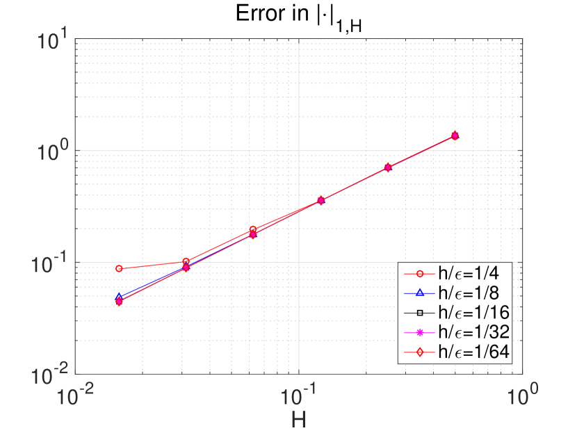
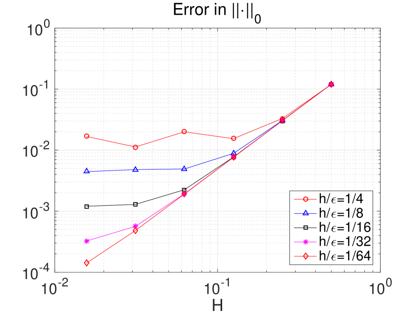
Figure 3: Result of the problem in Section 5.2. Errors in macro mesh-dependent norm (RT) and in $L^{2}$ norm (RB).

5.3 Example with noninteger-$\varepsilon$-multiple sampling domain and Dirichlet coupling

This example, which is originated from [1], is to investigate the effect of Dirichlet coupling on micro problems. Consider the multiscale elliptic problem with mixed boundary condition

$$-\nabla\cdot\Big{(}\mathbf{A}^{\varepsilon}({\mathbf{x}})\nabla u^{\varepsilon}({\mathbf{x}})\Big{)} =f({\mathbf{x}})\quad\mbox{in }\Omega=(0,1)^{2},$$

$$\left.u^{\varepsilon}\right|_{\Gamma_{D}} =0,$$

$$\left.\nu\cdot\mathbf{A}^{\varepsilon}\nabla u^{\varepsilon}\right|_{\Gamma_{N}} =0,$$

where $\Gamma_{D}=\{(x_{1},x_{2})~{}|~{}x_{1}=0\mbox{ or }1\}\cap\partial\Omega$ and $\Gamma_{N}=\partial\Omega\setminus\Gamma_{D}$. We use the multiscale coefficient tensor $\mathbf{A}^{\varepsilon}({\mathbf{x}})=\big{(}2+\cos(2\pi x_{1}/\varepsilon)\big{)}I$ where $\varepsilon=10^{-3}$, the associated homogenized tensor $\mathbf{A}^{0}({\mathbf{x}})=diag(\sqrt{3},2)$, and $f\equiv 1$ which admits the exact homogenized solution $u^{0}({\mathbf{x}})=-\frac{1}{2\sqrt{3}}x_{1}(x_{1}-1)$.

We use Dirichlet coupling on each micro problem. We have three options for sampling domain size $\delta$ which are not multiple of $\varepsilon$; $\delta=1.1\varepsilon$, $3.1\varepsilon$ and $\sqrt{\varepsilon}$. The last option is deduced from (35) for the optimal convergence. For each macro element 128 micro elements are used, a sufficiently large number, in order to guarantee that the micro error (32) can not disrupt the tendency of the total error, except the case of $\sqrt{\varepsilon}$ with 512.

We can observe that error varies depending on size of sampling domains. As shown in Figure 4, the bigger size of sampling domains gives the more accurate results.

$H$	$\delta=1.1\varepsilon$ (Diri.)	$3.1\varepsilon$ (Diri.)	$\sqrt{\varepsilon}$ (Diri.)
	${{\left|\kern-0.8611pt\left|\kern-0.8611pt\left|u^{0}-u_{H}\right|\kern-0.8611pt\right|\kern-0.8611pt\right|}}_{H}$
1/2	8.41E-02	8.34E-02	8.33E-02
1/4	4.22E-02	4.17E-02	4.17E-02
1/8	2.51E-02	2.14E-02	2.09E-02
1/16	1.50E-02	1.11E-02	1.04E-02
1/32	1.14E-02	6.33E-03	5.28E-03
	$\|u^{0}-u_{H}\|_{0}$
1/2	1.60E-02	1.41E-02	1.34E-02
1/4	5.07E-03	3.91E-03	3.33E-03
1/8	5.11E-03	2.29E-03	1.20E-03
1/16	3.56E-03	1.38E-03	3.57E-04
1/32	2.84E-03	1.03E-03	2.39E-04
	$\sup_{K_{\delta,i}}\|\mathbf{A}^{0}-\mathbf{A}^{0}_{K_{\delta,i}}\|_{F}$
1/2	1.59E-01	5.34E-02	1.16E-02
1/4	8.45E-02	2.97E-02	4.82E-03
1/8	1.78E-01	6.01E-02	1.64E-02
1/16	1.42E-01	4.79E-02	8.22E-03
1/32	1.74E-01	5.88E-02	1.55E-02

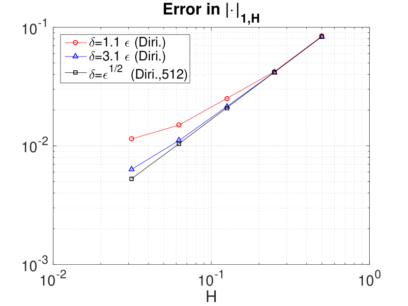
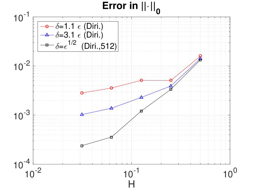
Figure 4: Result of the problem in Section 5.3, $\delta=1.1\varepsilon$, $3.1\varepsilon$, $\sqrt{\varepsilon}$. (RT) Error in macro mesh-dependent norm and (RB) in $L^{2}$ norm.

5.4 An example on a mixed domain

The last example is a problem on a domain which consists of distinct coefficients. Let $\Omega=(0,1)^{2}$ be decomposed of the two disjoint subdomains $\Omega_{1}=\big{\{}(x_{1},x_{2})\in\Omega~{}\big{|}~{}x_{1}>0.5\text{ and }x_{2}<0.5\big{\}}$ and $\Omega_{2}=\Omega\setminus\overline{\Omega_{1}}.$ We consider the second–order elliptic problem with the coefficient tensor

$$\mathbf{A}^{\varepsilon}({\mathbf{x}})=\begin{pmatrix}1.1+\delta_{k,1}\sin(2\pi{x_{1}}/{\varepsilon})&0\\ 0&1.1+\delta_{k,1}\sin(2\pi{x_{1}}/{\varepsilon})\end{pmatrix}\quad\text{if}\quad\mathbf{x}\in\Omega_{k}$$

where $\varepsilon=10^{-3}$, and the right hand side $f\equiv 0$. Here $\delta_{ij}$ denotes the standard Kronecker delta. We impose the homogeneous Neumann boundary condition on the upper and lower boundary, and the inhomogeneous Dirichlet boundary condition with values $1$ and $0$ on on the left and right boundaries, respectively. Any mesh used in this example consists of uniform squares. We applied the periodic coupling for micro problems with $\delta=\varepsilon$. By using the associated homogenized tensor

$$\mathbf{A}^{0}({\mathbf{x}})=\begin{cases}\begin{pmatrix}\sqrt{0.21}&0\\ 0&1.1\end{pmatrix}&\qquad\mbox{for }{\mathbf{x}}\in\Omega_{1},\\ \begin{pmatrix}1.1&0\\ 0&1.1\end{pmatrix}&\qquad\mbox{for }{\mathbf{x}}\in\Omega_{2},\end{cases}$$

the reference solution $u^{0}_{ref}$ on $512\times 512$ mesh is obtained.

Contour plots of the solutions are drawn in Figure 5 for comparison. The plot on top left is for the FEM solution $u^{\varepsilon}_{ref}$, and the top right plot is for the FEM solution $u^{0}_{ref}$ of the homogenized problem. Both solutions are obtained on $512\times 512$ uniform square mesh. The plot on bottom left is for the FEHMM solution $u_{H}$ from the macro mesh with $8\times 8$ uniform squares, and the micro mesh with $16\times 16$ uniform squares. The contour plots show the resemblance of the FEHMM solution to the solution of the homogenized problem as well as the solution of the original multiscale problem. The table shows error of FEHMM solutions to the reference solution in energy norm, and in $L^{2}$-norm. We can observe the reduction of error due to decreasing $H$ and $h$, but not as much as the purely periodic case.

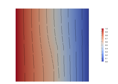
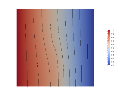
$H$	$h/\varepsilon$=1/16	1/32	1/64
	$\|u^{0}_{ref}-u_{H}\|_{0}$
1/2	9.45E-03	9.84E-03	9.97E-03
1/4	2.86E-03	2.83E-03	2.90E-03
1/8	1.53E-03	8.31E-04	8.20E-04
1/16	1.48E-03	4.11E-04	2.32E-04
1/32	1.50E-03	3.86E-04	1.06E-04
1/64	1.58E-03	3.91E-04	9.73E-05
	${{\left|\kern-0.8611pt\left|\kern-0.8611pt\left|u^{0}_{ref}-u_{H}\right|\kern-0.8611pt\right|\kern-0.8611pt\right|}}_{H}$
1/2	9.02E-02	9.07E-02	9.09E-02
1/4	5.32E-02	5.34E-02	5.35E-02
1/8	3.07E-02	3.04E-02	3.04E-02
1/16	1.78E-02	1.69E-02	1.69E-02
1/32	1.11E-02	9.32E-03	9.21E-03
1/64	8.31E-03	5.21E-03	4.97E-03

Figure 5: Result of the problem in Section 5.4. FEM solution $u^{\varepsilon}_{ref}$ (TL) and FEM solution $u^{0}_{ref}$ on $512\times 512$ uniform squares (TR). FEHMM solution $u_{H}$ using $8\times 8$ uniform squares as the macro mesh and $16\times 16$ uniform squares as the micro mesh (BL).

References

• [1] A. Abdulle. The finite element heterogeneous multiscale method: a computational strategy for multiscale pdes. GAKUTO International Series Mathematical Sciences and Applications, 31(EPFL-ARTICLE-182121):135–184, 2009.
• [2] A. Abdulle. Discontinuous Galerkin finite element heterogeneous multiscale method for elliptic problems with multiple scales. Math. Comp., 81(278):687–713, 2012.
• [3] A. Abdulle and Y. Bai. Reduced basis finite element heterogeneous multiscale method for high-order discretizations of elliptic homogenization problems. J. Comp. Phys., 231(21):7014–7036, 2012.
• [4] A. Abdulle and A. Nonnenmacher. A short and versatile finite element multiscale code for homogenization problems. Comput. Methods Appl. Mech. Engrg., 198(37):2839–2859, 2009.
• [5] A. Abdulle and A. Nonnenmacher. Adaptive finite element heterogeneous multiscale method for homogenization problems. Comput. Methods Appl. Mech. Engrg., 200(37):2710–2726, 2011.
• [6] A. Abdulle, E. Weinan, B. Engquist, and E. Vanden-Eijnden. The heterogeneous multiscale method. Acta Numerica, 21:1–87, 2012.
• [7] I. Babuška. Homogenization approach in engineering. In Computing methods in applied sciences and engineering, pages 137–153. Springer, 1976.
• [8] I. Babuška, G. Caloz, and J. E. Osborn. Special finite element methods for a class of second order elliptic problems with rough coefficients. SIAM J. Numer. Anal., 31(4):945–981, 1994.
• [9] D. Braess. Finite elements: Theory, fast solvers, and applications in solid mechanics. Cambridge University Press, 2007.
• [10] S. C. Brenner and L.-Y. Sung. Linear finite element methods for planar linear elasticity. Math. Comp., 59(200):321–338, 1992.
• [11] C. L. Bris, F. Legoll, , and A. Lozinski. MsFEM á la Crouzeix-Raviart for highly oscillatory elliptic problems. Chinese Annals of Mathematics, Series B, 34(1):113–138, 2013.
• [12] C. L. Bris, F. Legoll, , and A. Lozinski. An MsFEM type approach for perforated domains. SIAM Multiscale Modeling & Simulation, 12(3):1046–1077., 2014.
• [13] Z. Cai, J. Douglas, Jr., J. E. Santos, D. Sheen, and X. Ye. Nonconforming quadrilateral finite elements: A correction. Calcolo, 37(4):253–254, 2000.
• [14] Z. Cai, J. Douglas, Jr., and X. Ye. A stable nonconforming quadrilateral finite element method for the stationary Stokes and Navier-Stokes equations. Calcolo, 36:215–232, 1999.
• [15] D. Cioranescu and P. Donato. An introduction to homogenization, volume 17 of Oxford Lecture Series in Mathematics and its Applications, volume 4. The Clarendon Press Oxford University Press, New York, 1999.
• [16] M. Crouzeix and P. Raviart. Conforming and nonconforming finite element methods for solving the stationary Stokes equations. I. Rev. Française Automat. Informat. Recherche Opérationnelle Sér. Rouge, 7(R-3):33–75, 1973.
• [17] P. Degond, A. Lozinski, B. Muljadi, and J. Narski. Crouzeix-Raviart MsFEM with bubble functions for diffusion and advection-diffusion in perforated media. Communications in Computational Physics, 17(4):887–907, 2015.
• [18] J. Douglas, Jr., J. E. Santos, D. Sheen, and X. Ye. Nonconforming Galerkin methods based on quadrilateral elements for second order elliptic problems. ESAIM–Math. Model. Numer. Anal., 33(4):747–770, 1999.
• [19] W. E and B. Engquist. The heterogeneous multiscale methods. Communications in Mathematical Sciences, 1(1):87–132, 2003.
• [20] W. E, P. Ming, and P. Zhang. Analysis of the heterogeneous multiscale method for elliptic homogenization problems. J. Amer. Math. Soc., 18(1):121–156 (electronic), 2005.
• [21] Y. Efendiev, J. Galvis, and T. Y. Hou. Generalized multiscale finite element methods (GMsFEM). J. Comp. Phys., 251:116–135, 2013.
• [22] Y. Efendiev, J. Galvis, G. Li, and M. Presho. Generalized multiscale finite element methods: Oversampling strategies. International Journal for Multiscale Computational Engineering, 12(6), 2014.
• [23] Y. Efendiev and T. Y. Hou. Multiscale finite element methods: theory and applications, volume 4. Springer Science & Business Media, 2009.
• [24] Y. Efendiev, R. Lazarov, M. Moon, and K. Shi. A spectral multiscale hybridizable discontinuous Galerkin method for second order elliptic problems. Comput. Methods Appl. Mech. Engrg., 292:243–256, 2015.
• [25] Y. Efendiev and A. Pankov. Numerical homogenization of nonlinear random parabolic operators. Multiscale Modeling & Simulation, 2(2):237–268, 2004.
• [26] Y. R. Efendiev, T. Y. Hou, and X.-H. Wu. Convergence of a nonconforming multiscale finite element method. SIAM J. Numer. Anal., 37(3):888–910, 2000.
• [27] B. Engquist and P. E. Souganidis. Asymptotic and numerical homogenization. Acta Numerica, 17:147–190, 2008.
• [28] T. Y. Hou and X.-H. Wu. A multiscale finite element method for elliptic problems in composite materials and porous media. J. Comp. Phys., 134(1):169–189, 1997.
• [29] T. Y. Hou, X.-H. Wu, and Z. Cai. Convergence of a multiscale finite element method for elliptic problems with rapidly oscillating coefficients. Math. Comp., 68(227):913–943, 1999.
• [30] J. Hu and Z.-C. Shi. A new a posteriori error estimate for the Morley element. Numer. Math., 112:25–40, 2009.
• [31] J. Hu, Z.-C. Shi, and J. Xu. Convergence and optimality of the adaptive Morley element method. Numer. Math., 121:731–752, 2012.
• [32] T. J. R. Hughes, G. R. Feijóo, L. Mazzei, and J.-B. Quincy. The variational multiscale method—a paradigm for computational mechanics. Comput. Methods Appl. Mech. Engrg., 166(1-2):3–24, 1998.
• [33] P. Jenny, S. Lee, and H. Tchelepi. Multi-scale finite-volume method for elliptic problems in subsurface flow simulation. J. Comp. Phys., 187(1):47–67, 2003.
• [34] V. V. Jikov, S. M. Kozlov, and O. A. Oleinik. Homogenization of differential operators and integral functions. Springer-Verlag, Berlin, Heidelberg, New York, 1994.
• [35] S. Kim, J. Yim, and D. Sheen. Stable cheapest nonconforming finite elements for the Stokes equations. J. Comput. Appl. Math., 299:2–14, 2016.
• [36] C.-O. Lee, J. Lee, and D. Sheen. A locking-free nonconforming finite element method for planar elasticity. Adv. Comput. Math., 19(1–3):277–291, 2003.
• [37] C. S. Lee and D. Sheen. Nonconforming generalized multiscale finite element methods. J. Comput. Appl. Math., 311:215–229, 2017.
• [38] A. Lozinski, Z. Mghazli, , and K. Blal. Méthode des éléments finis multiéchelles pour le probléme de Stokes. Comptes Rendus Mathematique, 351(7):271–275, 2013.
• [39] S. Mao and Z.-C. Shi. High accuracy developed a superconvergence property for Morley element on a uniform rect-triangle. Adv. Comput. Math., 28(1):81–100, 2008.
• [40] L. S. D. Morley. The triangular equilibrium problem in the solution of plate bending problems. Aero. Quart., 19:149–169, 1968.
• [41] P. Muljadi, J. Narski, A. Lozinski, and P. Degond. Nonconforming multiscale finite element method for Stokes flows in heterogeneous media. Part I : Methodologies and numerical experiments. SIAM Multiscale Modeling & Simulation, 13(4):1146–1172, 2015.
• [42] C. Park. A study on locking phenomena in finite element methods. PhD thesis, Department of Mathematics, Seoul National University, Korea, Feb. 2002. Available at http://www.nasc.snu.ac.kr/cpark/papers/phdthesis.ps.gz.
• [43] C. Park and D. Sheen. $P_{1}$-nonconforming quadrilateral finite element methods for second-order elliptic problems. SIAM J. Numer. Anal., 41(2):624–640, 2003.
• [44] C. Park and D. Sheen. A quadrilateral Morley element for biharmonic equations. Numer. Math., 124(2):395–413, 2013.
• [45] R. Rannacher and S. Turek. Simple nonconforming quadrilateral stokes element. Numerical Methods for Partial Differential Equations, 8(2):97–111, 1992.
• [46] E. Sanchez-Palencia. Non-homogeneous Media and Vibration Theory, volume 127. Springer-Verlag, Berlin and New York, 1980.
• [47] D. Shi and P. Xie. Morley type non–$C^{0}$ nonconforming rectangular plate finite elements on anisotropic meshes. Numer. Methods Partial Differential Equations, 26:723–744, 2010.
• [48] G. Strang and G. J. Fix. An analysis of the finite element method, volume 212. Prentice-hall Englewood Cliffs, NJ, 1973.
• [49] S. Turek. Efficient solvers for incompressible flow problems, volume 6 of Lecture Notes in Computational Science and Engineering. Springer, Berlin, 1999.
• [50] J. Yim and D. Sheen. $P_{1}$–nonconforming quadrilateral finite element space with periodic boundary conditions:
Part I. Fundamental results on dimensions, bases, solvers, and error analysis.
this jouranl. submitted.