Estimating time constants of the RTS noise in semiconductor devices: a complete description of the observation window in the time domain

Abstract

We obtained a semi-analytical treatment obtaining estimators for the sample variance and variance of sample variance for the RTS noise. Our method suggests a way to experimentally determine the constants of capture and emission in the case of a dominant trap and universal behaviors for the superposition from many traps. We present detailed closed-form expressions corroborated by MC simulations. We are sure to have an important tool to guide developers in building and analyzing low-frequency noise in semiconductor devices.

1 Introduction

Knowing the so-called low-frequency (LF) noise [1, 2] means understanding the stochastic process of the capture/emission mechanisms by traps. Such phenomena can be due to one only single dominant trap or dominated by multiple random telegraph signals (RTS) due to many traps, in semiconductor-dielectric interfaces found in CMOS transistors [3, 4]. Both situations are important and their study is essential, and of technological interest. To model such a process, we can imagine a straightforward mechanism described by Fig. 1 (a)

In this scheme, a trap captures one charge carrier between the time $t$ and $t+\delta t$, with probability

$$p(0\rightarrow 1)\delta t\approx\frac{1}{\tau_{c}}\delta t\text{.}$$ (1)

This charge carrier returns to the inversion layer with a probability

$$p(1\rightarrow 0)\delta t\approx\frac{1}{\tau_{e}}\delta t$$ (2)

at the same time interval. Here $\tau_{c}$ and $\tau_{e}$ are capture and emission constants, respectively. Generally, we make $\delta t=1$ u.t. (unit of time), imagined as a minimal quantity in a typical Monte Carlo (MC) simulation, or simply 1 MC step. When a trap captures a charge carrier, one observes a fluctuation of magnitude $\Delta v$ in the voltage, and one subtracts this same value in the emission of this charge carrier to the inversion layer.

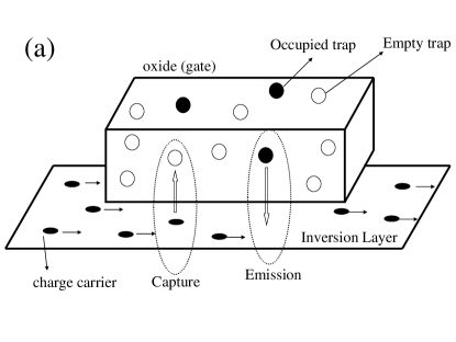
Figure 1: (a) A simplification of a CMOS transistor (b) Simulation of the threshold voltage in a CMOS dispositive considering 1, 3, and 50 traps, represented by (I), (II), and (III) respectively.

Fig. 1 (b) shows the threshold voltage considering the contribution of one, three, and fifty traps considering simple MC simulations following the prescription that we previously defined. In this case, we consider the amplitude $\Delta v$ is the same for all traps in this simple experiment. We can observe that the sum of these fluctuations compose exciting patterns, and its understanding is essential to developing reliable devices.

The phenomenology of random telegraph signals considers that the distributions:

$$P_{0(1)}(t)=\frac{1}{\tau_{e(c)}}e^{-t/\tau_{e(c)}}$$ (3)

describe the probability density functions which govern the residence time on the different states $\sigma_{i}=0(1)$, captured/emitted respectively, where the time constants:

$$\tau_{e(c)}=\int\limits_{0}^{\infty}tP_{0(1)}(t)dt\text{,}$$ (4)

are here translated as averaged capture time ($\tau_{c}$), and averaged emission time ($\tau_{e}$) respectively.

Although many works consider the analysis in the frequency domain of RTS (to cite a few ones [5, 6, 7, 8, 9, 10]), on the other hand, time-domain analysis (see for example [11, 12, 13, 14]) deserves more attention from researchers in this kind of modeling. Time-domain analysis is important for example to understand the degradation phenomena in semiconductor devices from experimental [15], and theoretical point of view [16]. However, analysis in the time domain does not explore studies about the observation window, which seems to be an important parameter [17, 18].

In this paper, we develop a very detailed approach to study, in time domain regime, ways to characterize the RTS noise using a semi-analytical treatment and Monte Carlo (MC) simulations. We first developed an approach for the case of a single dominant trap. We analyzed the noise variance per time window and the variance of the sample variance as a function of time window size. This analysis allows developers, for example, to estimate the constants $\tau_{c}$ and $\tau_{e}$ independently, since we present closed-form equations for these two quantities based on the hypothesis that MC simulations, supposedly imitating an experiment, supply as input the steady-state of the variance and the point that maximizes the variance of the variance.

In addition, we also performed an extrapolation of this result for the contribution of many traps. We show that variance per window shows a universal linear behavior, as suggested by previous contributions [17, 18]. However these works import previous results obtained in frequency domain [4] and therefore with parameters not directly extracted.

We performed an analysis entirely made in the time domain in this current contribution, which leads to a universal behavior with easily checked parameters and that presents an excellent agreement with MC simulations.

Finally, we also show a universal behavior for the variance of the variance, suggesting a regime where this amount does not depend on the time window, a result that literature never observed.

In the next section, we present our semi-analytical modeling. The penultimate section presents some results by comparing MC simulations with these semi-analytical predictions. Finally, in the last section, some summaries and conclusions are presented.

2 Semi-analytical predictions

In this section, we will deduce some formulas for the sample variance and for the variance of the sample variance, which are used to characterize RTS and mainly to allow that we can compute the constants $\tau_{c}$ and $\tau_{e}$. We first prepare an analysis for one only dominant trap. After, we deduce some expressions considering the contribution of many traps for the noise.

2.1 Single trap

For a single trap, we calculate the threshold voltage average as:

$$\left\langle v\right\rangle=p_{0}\cdot 0+p_{1}\delta v\text{.}$$ (5)

Here $p_{0}$ denotes the probability that an electron is not trapped, while $p_{1}$ is the probability that an electron is trapped. In this situation, there is a contribution of $\delta v$ to the voltage, while we consider that in the first situation, the voltage variation is 0. Thus $s=\frac{v}{\Delta v}$ is a Bernoulli random variable, but only when the observation time of the noise: $T>>\tau_{c},\tau_{e}$, since, in this scale, $p_{0}$, and $p_{1}$ are given by:

$$p_{0} = \frac{\tau_{e}}{\tau_{e}+\tau_{c}}$$ (6)

$$p_{1} = \frac{\tau_{c}}{\tau_{e}+\tau_{c}}\text{,}$$

such that $p_{0}+p_{1}=1$.

Thus, $\left\langle v\right\rangle=\frac{\tau_{c}}{\tau_{e}+\tau_{c}}\delta v$. The dispertion (variance) of the voltage change  is so calculated by first calculating the second moment:

$$\left\langle v^{2}\right\rangle=0p_{0}+\frac{\tau_{c}}{\tau_{e}+\tau_{c}}(\delta v)^{2}$$ (7)

which yields to $var(v)=$ $\left\langle v^{2}\right\rangle-\left\langle v\right\rangle^{2}=\frac{\tau_{e}\tau_{c}}{\left(\tau_{e}+\tau_{c}\right)^{2}}(\delta v)^{2}$. We denote:

$$var_{\infty}=\frac{var(v)}{(\delta v)^{2}}=\frac{\tau_{e}\tau_{c}}{\left(\tau_{e}+\tau_{c}\right)^{2}}$$ (8)

Since $\Delta v$ is the voltage amplitude of a single trap, we can make $\delta v=1$ in our calculations or think our calculations scale with this quantity for the case of one single trap for the sake of simplicity.

In order to analyze the effects of finite size time $\Delta$, to compute $var(v)$, we suggest to calculate $var(v)$ for a specific time window that can change from $\Delta<\tau$, where: $\frac{1}{\tau}=\frac{1}{\tau_{e}}+\frac{1}{\tau_{c}}$ up to $\Delta=T$. In our results always $T>>\tau\in[\min\left\{\tau_{e},\tau_{e}\right\},\max\left\{\tau_{e},\tau_{e}\right\}]$.

Heuristically, we can obtain $var(v|\Delta)$, the expected variance for an arbitrary time window of size $\Delta$. One supposes that when $\Delta<<\tau$, $var(v)\rightarrow 0$, there is no time for occurrences of captures or emissions. On the other hand, for $\Delta>>\tau$, $var(v)\rightarrow var_{\infty}$. Thus we performed a detailed study in literature, and we tested many functions to perform the transient between these two regimes. We conclude that transient must behave according to a sigmoidal function.

The simple sigmoidal behavior, that reproduces these two limits, is the known Hill-Langmuir [19, 20] equation:

$$f(\Delta)=\frac{\Delta^{n}}{\Delta^{n}+\Delta_{c}}\text{,}$$ (9)

where $n$ and $\Delta_{c}$ are constants to be fitted. A simple choice is only to perform the most straightforward form: $n=1$, in order to consider a function with only available parameter $\Delta_{c}$, that, as we will observe, has the central role in our modeling.

Thus, aggregating the last information, we obtain the conjecture

$$var(v|\Delta)=\left\langle v^{2}|\Delta\right\rangle-\left\langle v|\Delta\right\rangle^{2}=\frac{\tau_{e}\tau_{c}\left(\tau_{e}+\tau_{c}\right)^{-2}}{\left[1+\left(\frac{\Delta_{c}}{\Delta}\right)\right]}\text{,}$$ (10)

which yields the expected limits: $var(v|0)=0$ e $\lim_{\Delta\rightarrow\infty}var(v|\Delta)=\frac{\tau_{e}\tau_{c}}{\left(\tau_{e}+\tau_{c}\right)^{2}}$, where

$$\left\langle x|\Delta\right\rangle=xp_{1}(\Delta)+0(1-p_{1}(\Delta))=xp_{c}(\Delta)\text{.}$$ (11)

Thus we hypothesize is that the formulae 10 works for intermediate values of $\Delta$, as we will check. Eq. 10 also allows, for example, to obtain closed-form expressions for $p_{0}(\Delta)$ and $p_{1}(\Delta)$, which correspond to the probabilities of remaining in the states 0 and 1, respectively, as a function of $\Delta$, just making:

$$p_{1}(\Delta)\left[1-p_{1}(\Delta)\right]=\dfrac{\tau_{e}\tau_{c}\left(\tau_{e}+\tau_{c}\right)^{-2}}{\left[1+\left(\frac{\Delta_{c}}{\Delta}\right)\right]}\text{.}$$ (12)

Another hypothesis that seems very reasonable, and which we will verify in this paper, is to consider that $\Delta_{c}$ linearly scales with $\tau$, i.e., $\Delta_{c}=b\tau$, where $b$ is a constant. Thereby, under these considerations, solving the equation 12, one has

$$p_{1}(\Delta)=\frac{1}{2\left(\tau_{e}+\tau_{c}\right)}\left(\tau_{e}+\tau_{c}\pm\sqrt{\frac{1}{(1+b\frac{\tau}{\Delta})}(\tau_{e}^{2}+\tau_{c}^{2}-2\tau_{e}\tau_{c}+\frac{b\tau\tau_{e}^{2}+b\tau\tau_{c}^{2}+2b\tau\tau_{e}\tau_{c}}{\Delta})}\right)$$ (13)

The signal says a important point, if $\tau_{e}>\tau_{c}$, the negative signal leads to $\lim_{\Delta\rightarrow\infty}p_{1}(\Delta)=\frac{\tau_{c}}{\tau_{c}+\tau_{e}}$, while if $\tau_{c}>\tau_{e}$, the positive signal leads to $\lim_{\Delta\rightarrow\infty}p_{1}(\Delta)=\frac{\tau_{c}}{\tau_{c}+\tau_{e}}$, and sure if $\tau_{c}=\tau_{e}$, one has $\lim_{\Delta\rightarrow\infty}p_{1}(\Delta)=\frac{1}{2}$. It is also important to observe that $\lim_{\Delta\rightarrow 0}p_{1}(\Delta)=0$ for the negative and $\lim_{\Delta\rightarrow 0}p_{1}(\Delta)=1$ for positive, which makes sense since the state can start with 0 or 1.

Since we understand this semi-analytical treatment, we can imagine estimating $var(\Delta)$, from a computational/numerical point of view, which we performed according to sample variance for a specific ($k$-th) time window by

$$\widehat{var}_{k}(v|\Delta)=\frac{1}{\Delta-1}\sum_{i=k\Delta+1}^{(k+1)\Delta}(s_{i}-\overline{s}^{(k)})^{2}$$ (14)

where $s_{i}=0,1$ is Bernoulli random variable, and $\overline{s}^{(k)}=\frac{1}{\Delta}\sum_{i=k\Delta+1}^{(k+1)\Delta}s_{i}$. Thus, since we sliced $T$ in $\left\lfloor T/\Delta\right\rfloor$ time windows of size $\Delta$, computing the average variance:

$$\widehat{var}(v|\Delta)=\frac{1}{\left\lfloor T/\Delta\right\rfloor}\sum_{k=1}^{\left\lfloor T/\Delta\right\rfloor}var_{k}(v|\Delta)\text{,}$$ (15)

which is a more refined estimate for the theoretical value expressed by Eq. 10:

And about the dispersion of $var_{k}(v|\Delta)$? We can numerically determine it by computing

$$\widehat{var}(var_{k}(v|\Delta))=\frac{1}{\left\lfloor T/\Delta\right\rfloor-1}\sum_{k=1}^{\left\lfloor T/\Delta\right\rfloor}\left(var_{k}(v|\Delta)-\widehat{var}(v|\Delta)\right)^{2}\text{.}$$ (16)

However, the estimation theory suggests that an estimator for $\widehat{var}(var_{k}(\Delta))$ has the form: $2\frac{var^{2}(v|\Delta)}{\Delta-1}$ (see for example [21]). However considering that some adittional “ingredients” is necessary, we consider for convenience:

$$var(var(v|\Delta))\approx\frac{K(\tau)var^{2}(v|\Delta)}{\Delta}\text{,}$$ (17)

where $K(\tau)$ is a “ad-hoc” constant that depends only on $\tau$, built-in in our analysis. From semi-analytical formulae for $var(v|\Delta)$ (Eq. 10), we propose:

$$var(var(v|\Delta))=K(\tau)\frac{\tau_{e}^{2}\tau_{c}^{2}\left(\tau_{e}+\tau_{c}\right)^{-4}}{\Delta\left[1+\left(\Delta_{c}/\Delta\right)\right]^{2}}\equiv\frac{\tau_{e}^{2}\tau_{c}^{2}K(\tau)\Delta}{\left(\tau_{e}+\tau_{c}\right)^{4}\left[\Delta+\Delta_{c}\right]^{2}}\text{.}$$ (18)

We can verify that such quantity has a maximum in $\frac{d\ }{d\Delta}var(var(v|\Delta))=0$, resulting in$\frac{1}{\left(\Delta+\Delta_{c}\right)^{2}}-\frac{2\Delta}{\left(\Delta+\Delta_{c}\right)^{3}}=0$, and yielding $\Delta_{\max}=\Delta_{c}$, which behaves as $b\tau$ (a hypothesis to be checked in the section corresponding to our results).

At this point, it is important to highlight some considerations. If this approach is correct, it has important implications. From experimental results we can experimentally determine the parameter $\widehat{var}_{\infty}$ which is numerically equal $\dfrac{\tau_{e}\tau_{c}}{\left(\tau_{e}+\tau_{c}\right)^{2}}$, and the parameter $\widehat{\Delta}_{c}$, that is, according with our modeling, numerically equal to $b\frac{\tau_{e}\tau_{c}}{\left(\tau_{e}+\tau_{c}\right)}$. Solving these equations, we can obtain, directly and independently $\tau_{c}$ and $\tau_{e}$, which are the constants that characterize the noise:

$$\tau_{c}=\frac{\widehat{\Delta}_{c}}{2b\widehat{var}_{\infty}}(1\pm\sqrt{1-4\widehat{var}_{\infty}})$$ (19)

and

$$\tau_{e}=\frac{\widehat{\Delta}_{c}}{2b\widehat{var}_{\infty}}(1\mp\sqrt{1-4\widehat{var}_{\infty}})$$ (20)

as a function only on experimental parameters:$\ \widehat{\Delta}_{c}$ and $\widehat{var}_{\infty}$ respectively given by the inflection point and steady-state value of noise variance. Observe that the equations 19 and 20 also clearly show the symmetry between these two constants. In this case, the only necessary task is to numerically show our assumptions in the section corresponding to our results. In the following subsection, we performed an analysis of variance, and variance of variance, considering a situation of a large number of traps.

2.2 Analysis with many traps

In this case, we can assume that $V=\sum_{i=1}^{N_{tr}}v_{i}$ is the contribution from $N_{tr}$ traps for the voltage, thus

$$\begin{array}[]{lll}var(V|\Delta)&=&var(\sum_{i=1}^{N_{tr}}v_{i}|\Delta)\\ &&\\ &=&\left\langle\left.\left(\sum_{i=1}^{N_{tr}}v_{i}\right)^{2}\right|\Delta\right\rangle-\left\langle\left.\left(\sum_{i=1}^{N_{tr}}v_{i}\right)\right|\Delta\right\rangle^{2}\\ &&\\ &=&\sum_{i=1}^{N_{tr}}\left(\left\langle v_{i}^{2}|\Delta\right\rangle-\left\langle v_{i}|\Delta\right\rangle^{2}\right)+\sum_{i\neq j}\left(\left\langle v_{i}v_{j}|\Delta\right\rangle-\left\langle v_{i}|\Delta\right\rangle\left\langle v_{j}|\Delta\right\rangle\right)\\ &&\\ &=&\sum_{i=1}^{N_{tr}}\left(\left\langle v_{i}^{2}|\Delta\right\rangle-\left\langle v_{i}|\Delta\right\rangle^{2}\right)\\ &&\\ &=&\sum_{i=1}^{N_{tr}}var(v_{i}|\Delta)\text{,}\end{array}$$ (21)

since the traps are supposedly uncorrelated: $\left\langle v_{i}v_{j}|\Delta\right\rangle=\left\langle v_{i}|\Delta\right\rangle\left\langle v_{j}|\Delta\right\rangle$.

Now it is important to consider that $\tau_{c}$ and $\tau_{e}$ are written as [1]:

$$\tau_{c} = 10^{p}(1+e^{q})$$ (22)

$$\tau_{c} = 10^{p}(1+e^{-q}),$$

where $q$ and $p$ are uniformly distributed. Here $q\in[-Q,Q]$, while $p\in[p_{\min},p_{\max}]$, where in this paper we use $Q=2$ and $p_{\min}=1$, and $p_{\max}=7$ which are values experimentally plausible.

Defining

$$\left\langle x\right\rangle_{q,p,\Delta v}=\frac{1}{2Q(p_{\max}-p_{\min})}\int_{0}^{\infty}\int_{-Q}^{Q}\int_{p_{\min}}^{p_{\max}}w(\delta v)x(p,q)dpdqd(\delta v),$$ (23)

where $w(\delta v)$ is the probability density function of the threshold voltage of the traps.

We can calculate the average variance considering the contribution of $N_{tr}$ traps:

$$\begin{array}[]{lll}\left\langle var(V|\Delta)\right\rangle_{q,p,\delta v}&=&\sum_{i=1}^{N_{tr}}\left\langle var(v_{i}|\Delta)\right\rangle_{q,p,\delta v}\\ &&\\ &=&N_{tr}\left\langle var(v|\Delta)\right\rangle_{q,p,\delta v}\\ &&\\ &=&\frac{N_{tr}\left\langle(\delta v)^{2}\right\rangle}{4Q(p_{\max}-p_{\min})}\int_{-Q}^{Q}\frac{dq}{(1+\cosh q)}\int_{p_{\min}}^{p_{\max}}\frac{dp}{1+\frac{b}{\Delta}10^{p}}\\ &&\\ &=&\frac{N_{tr}\left\langle(\delta v)^{2}\right\rangle}{2Q(p_{\max}-p_{\min})}\tanh\left(\frac{Q}{2}\right)\left[(p_{\max}-p_{\min})-\frac{1}{\ln 10}\ln\left(\frac{\Delta+b10^{p_{\max}}}{\Delta+b10^{p_{\min}}}\right)\right]\end{array}$$ (24)

with

$$\left\langle(\delta v)^{2}\right\rangle=\int_{0}^{\infty}(\delta v)^{2}w(\delta v)d(\delta v)$$ (25)

You also can consider that the number of traps in a sample follows a poisson distribution $p_{\lambda}(N_{tr})=\lambda^{N_{tr}}\frac{e^{-\lambda}}{N_{tr}!}$with rate $\overline{N_{tr}}=\sum_{N_{tr}=0}^{\infty}N_{tr}p(N_{tr})$. And in this case the variance considering an average over many samples, is presented only by changing $N_{tr}$ by $\overline{N_{tr}}$:

$$\overline{\left\langle var(V)\right\rangle_{q,p,\delta v}}=\frac{N_{dec}\left\langle(\delta v)^{2}\right\rangle}{2Q}\tanh\left(\frac{Q}{2}\right)\left[(p_{\max}-p_{\min})-\frac{1}{\ln 10}\ln\left(\frac{\Delta+b10^{p_{\max}}}{\Delta+b10^{p_{\min}}}\right)\right]\text{,}$$ (26)

where $N_{dec}=\overline{N_{tr}}/(p_{\max}-p_{\min})$.

In this case, MC simulations for a fixed and large $N_{tr}$ substituted in this equation by $\overline{N_{tr}}$ must corroborate this semi-analytical result. Similarly from our previous calculations we calculated the variance of variance from a superposition of $N_{tr}$ traps:

$$\begin{array}[]{lll}var(var(V|\Delta))&=&\left\langle\left(var(\sum_{i=1}^{N_{tr}}v_{i}|\Delta)\right)^{2}\right\rangle_{\Delta}-\left\langle var(\sum_{i=1}^{N_{tr}}v_{i}|\Delta)\right\rangle_{\Delta}^{2}\\ &&\\ &=&\sum_{i=1}^{N_{tr}}\left\langle var(v_{i}|\Delta)^{2}\right\rangle_{\Delta}-\left\langle var(v_{i}|\Delta)\right\rangle_{\Delta}^{2}+\\ &&\\ &&\sum_{i\neq j}^{N_{tr}}\left\langle var(v_{i}|\Delta)var(v_{j}|\Delta)\right\rangle_{\Delta}-\left\langle var(v_{i}|\Delta)\right\rangle\left\langle var(v_{j}|\Delta)\right\rangle_{\Delta}\\ &&\\ &=&\sum_{i=1}^{N_{tr}}\left\langle var(v_{i}|\Delta)^{2}\right\rangle_{\Delta}-\left\langle var(v_{i}|\Delta)\right\rangle_{\Delta}^{2}\\ &&\\ &=&\sum_{i=1}^{N_{tr}}var(var(v_{i}|\Delta))\end{array}$$ (27)

since $\left\langle var(v_{i}|\Delta)var(v_{j}|\Delta)\right\rangle_{\Delta}=\left\langle var(v_{i}|\Delta)\right\rangle\left\langle var(v_{j}|\Delta)\right\rangle_{\Delta}$. The problem here stays in our ignorance about $K(\tau)$ in Eq. 18. The simple choice is simply to suppose a linear dependence: $K(\tau)=\gamma\tau=\gamma 10^{p}$, and following exactly as

$$\begin{array}[]{ccc}\overline{\left\langle var(var(V|\Delta))\right\rangle_{q,p,\Delta v}}&=&\frac{N_{dec}\gamma\Delta}{4Q}\left\langle(\delta v)^{4}\right\rangle\int_{-Q}^{Q}\frac{dq}{(1+\cosh q)^{2}}\int_{p_{\min}}^{p_{\max}}\frac{10^{p}}{\left[\Delta+b10^{p}\right]^{2}}dp\\ &&\\ &=&\frac{N_{dec}\gamma\Delta}{6Q\ln 10}\left\langle(\delta v)^{4}\right\rangle\frac{\sinh Q(\cosh Q+2)}{(\cosh Q+1)^{2}}\cdot\frac{10^{p_{\max}}-10^{p_{\min}}}{(b10^{p_{\max}}+\Delta)(b10^{p_{\min}}+\Delta)}\end{array}$$ (28)

where $\left\langle(\delta v)^{4}\right\rangle=\int_{0}^{\infty}(\delta v)^{4}w(\delta v)d(\delta v)$.

We will present our results divided into two parts: I – Single trap and II – Many traps, presented in the following.

3 Results Part I: Single trap

Let us start with simple experiments that corroborate our semi-analytical close-form expressions from Eqs. 10 and 18. Keeping $\tau_{c}=1000$ u.t. (unit of time), we performed MC simulations changing $\tau_{e}$. In these simulations we used a total of $T=10^{7}$ u.t. In our simulations as previously reported 1 u.t = 1 MC step. In Fig. 2 we show the sample variance for the particular cases $\tau_{e}=2000$ u.t and $\tau_{e}=4000$ u.t. We show the MC simulations (points) according to Eq. 15 compared with our semi-analytical result (Eq. 10) red curve.

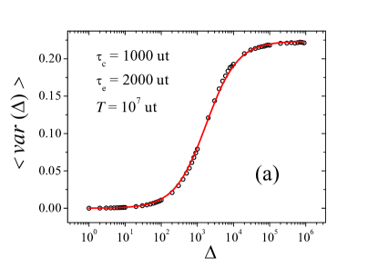
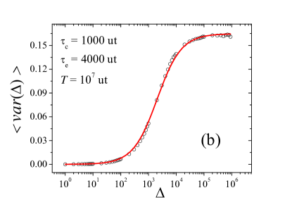
Figure 2: (a) The verage variance as a function of the time window. Here, we used $\tau_{c}=1000$ and $\tau_{e}=2000$. (b) The average variance as a function of time window when $\tau_{c}=1000$ and $\tau_{e}=4000$. Points correspond to MC simulations while the red line corresponds to our semi-analytical result according to Eq. 10

We observe a excellent agreement between MC and our semi-analytical result. It is important to observe that we numerically obtain $\tau_{e}\tau_{c}\left(\tau_{e}+\tau_{c}\right)^{-2}\approx 0.223$ for $\tau_{c}=1000$ u.t and $\tau_{c}=2000$ u.t in comparison with exact result: $1000\times 2000\times\left(3000\right)^{-2}=\allowbreak 0.2\overline{2}$ and $\tau_{e}\tau_{c}\left(\tau_{e}+\tau_{c}\right)^{-2}\approx 0.165$ for $\tau_{c}=1000$ u.t and $\tau_{c}=4000$ u.t, which corroborates the exact value: $0.16$. The same fits also lead to $\Delta_{c}=1735$ u.t and $\Delta_{c}=2050$ u.t respectively.

In order to check such estimates, we perform MC simulations by calculating $var(var_{k}(\Delta))$ numerically by Eq. 16. Thus we fit these results with function

$$f(\Delta)=k_{\max}\frac{\Delta}{\left(\Delta+\Delta_{c}\right)^{2}}$$ (29)

according to predicted by Eq. 18. Here $k_{\max}$ is a constant only to adjust the high of the peak. Thus, using the values of $\Delta_{c}$ we can observe the good agreement between MC simulations (points) and our semi-analytical prediction (red continuous curve) in Fig. 3.

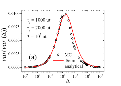
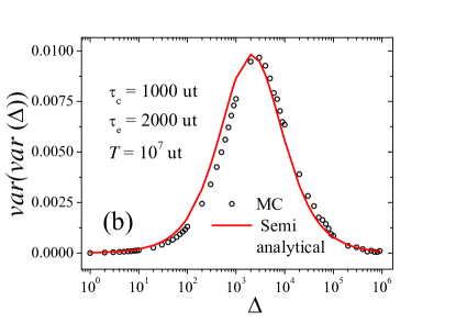
Figure 3: (a) The variance of sample variance as a function of time window: $\tau_{c}=1000$ and $\tau_{e}=2000$. (b) The variance of sample variance as a function of time window: $\tau_{c}=1000$ and $\tau_{e}=4000$. Points correspond to MC simulations while red line correspond to fit with Eq. 18

We observe the collapse of curves for different $\tau_{c}$ and $\tau_{e}$ if we divide the time window by $\tau$ and if we multiply the noise variance by $(\tau_{c}+\tau_{e})^{2}/\tau_{c}\tau_{e}$. The plots for the average variance and sample variance of variance are shown respectively in Fig. 4.

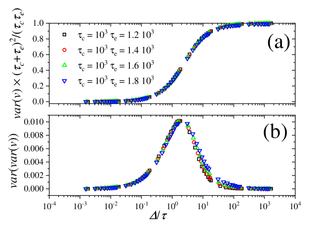
Figure 4: Collapse for different values of $\tau_{e}$ and $\tau_{c}$. (a) Average of the sample variance (b) Variance of the variance.

To complete the validation of the process, which allows for example that we can calculate $\tau_{c}$ and $\tau_{e}$ from experimental results through Eqs. 19 and 20, we need to establish how $\Delta_{c}$ depends on $\tau_{c}$ and $\tau_{e}$. More precisely, we need to show our assumption in this paper that is $\Delta_{c}=b\tau$. Thus considering $\tau_{c}=1000$ we change $\tau_{e}$, for that pair $\tau_{c}$ and $\tau_{e}$ we estimate $\Delta_{c}$. Thus we plot $\Delta_{c}$ as function of $\tau=\frac{\tau_{e}\tau_{c}}{\left(\tau_{e}+\tau_{c}\right)}$. Fig. 5 shows a robust linear behavior, corroborating the hypothesis $\Delta_{c}=b\ \tau$. The inset plot is only a highlight for the selected region.

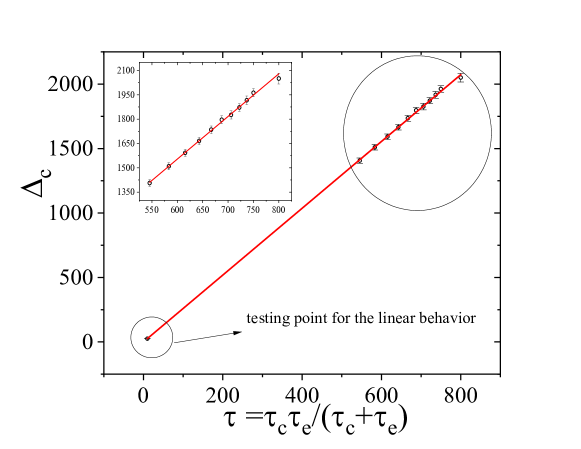
Figure 5: Linear behavior of $\Delta_{c}$ as a function of $\tau$. We use a testing point to show that linear behavior is robust for an extensive range in $\tau$. The inset plot is only a highlight for the selected region.

The first isolated point (corresponding to $\tau_{e}=10$) in order to show that the linear behavior is robust indeed. The linear fit leads to $b=2.62\pm 0.04$ and corroborates the hypothesis of our modeling for one trap.

4 Results Part II: Many traps

We performed MC simulations considering the contribution of many traps for the noise. Since that distribution $w(\delta v)$ is not known, we make $\left\langle(\delta v)^{2}\right\rangle$ and $\left\langle(\delta v)^{4}\right\rangle$ identically equal to 1, for the sake of simplicity, or we should imagine that amounts divided by these moments, which is not a technical problem here.

We considered simulations with $N_{tr}=10$, $20$, $30$, $40$, $50$, and $100$. In Figs. 6 (a) and (b). In Fig. 6 (a) we show our MC simulations for different number of traps, while in Fig. 6 (b) a comparison between MC simulations and our semi-analytical approach given by Eq. 24 is presented for the larger number of traps studied: $N_{tr}=100$.

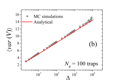
Figure 6: (a) The average variance for many traps via MC simulations. Analysis of the different number of traps (b) Selection of de case of $N_{tr}=100$ traps by extracting the first occurrences. We observe an excellent agreement between MC and our semi-analytical approach.

We observe an excellent agreement between the MC simulations and our semi-analytical approach. We can obtain a simple closed-form if we consider a seemingly crude approximation. Let us imagine a situation of a intermediate time window, where $\Delta>>10^{p_{\min}}$ but $\Delta<<10^{p_{\max}}$. In this case

$$\ln\left(\frac{\Delta+b10^{p_{\max}}}{\Delta+b10^{p_{\min}}}\right)\approx\ln b+p_{\max}\ln 10-\ln\Delta$$

And from Eq. 24 one has that

$$\left\langle var(V|\Delta)\right\rangle_{q,p,\delta v}\approx A+B\ln\Delta$$ (30)

where $A=\zeta N_{dec}$ and$\ B=\xi N_{dec}$, with

$$\zeta=-\frac{1}{2Q}\tanh\left(\frac{Q}{2}\right)\left[p_{\min}+\log b\right]$$ (31)

and

$$\xi=\frac{1}{2Q\ln 10}\tanh\left(\frac{Q}{2}\right)$$ (32)

Taking advantage of the results used for the Fig. 6 (a) we perform linear fits of $\left\langle var(V|\Delta)\right\rangle_{q,p,\delta v}$ as function of $\ln\Delta$ for the different values of $N_{tr}$.

Let us concentrate in the slope, i.e., the coefficient $B$ due to its greater importance. Thus we obtain $B$ for the different values of $N_{tr}$ as shown in Fig. 7 (a), (b), and (c) shows the linear behavior expected by Eq. 30 for respectively $N_{tr}=10$, $50$, and $100$. The red continuous curves correspond to linear fits. The same linear behavior is observed for $N_{tr}=20$, $30$, and $40$ (omitted by saving space).

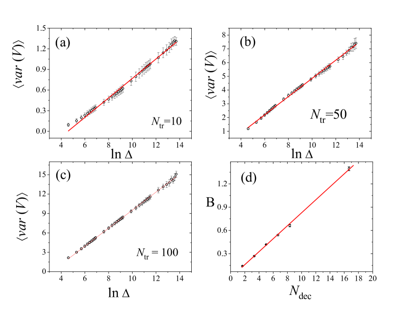
Figure 7: (a) The average as a function of $\ln\Delta$ for $N_{tr}=10$. The continuous curve corresponds to a linear fit. Plots (b) and (c) correspond to the same one performed in the plot (a) but for $N_{tr}=50$ and $100$ respectively. Finally, plot (d) corresponds to $B$ as a function of $N_{dec}$. We also observe an expected linear behavior where the slope corresponds to $\xi$.

Fig. 7 (d) shows exactly the slope $B$ obtained for these plots as function of $N_{dec}$. A linear fit also is performed and the slope must correspond to $\xi$ according to Eq. 32. The slope leads to: $\xi_{MC}=0.084\,6\pm 0.0012$. Using the values $Q=2$, $p_{\min}=1$, $p_{\max}=7$, one obtains:

$$\xi_{theor}=\frac{\tanh(1)}{4}\frac{1}{\ln 10}=0.0827,$$ (33)

 which agrees with $\xi_{MC}$ considering two uncertainty bars. In summary, the Eq. 30 is indeed correct by showing that variance of many traps behaves linearly on the logarithm of time window in RTS with slope expressed by Eq. 32.

Finally, let us consider the case of the variance of variance considering the contribution of many traps. We start with a “pedagogical” situation where we look at the situation of two and three traps in the sample $(N_{tr}=2$ and $3$).

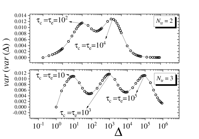
Figure 8: The variance of sample variance as a function of the time window considering (a) $N_{tr}=2$ traps, and (b) $N_{tr}=3$ traps. We averaged over $N_{run}=20$ different runs.

We can observe two peaks and three peaks, respectively, which is intuitive since for one trap, we observed a peak in $\Delta_{c}=b\tau$, and traps with different constants lead to peaks in the respective values. And about a large number of traps? Is the Eq. 28 valid? Is it compatible with MC simulations?

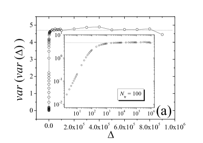
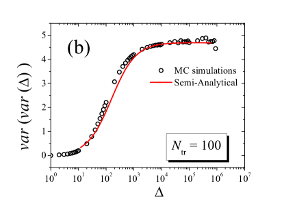
Figure 9: The variance of sample variance as a function of the time window considering many traps: $N_{tr}=100$. Plot (a) describes the situation on a linear scale. The inset plot corresponds to the same plot on a log-log scale. Plot (b) considers the same plot with a semi-log scale (log in the time window axis). We compared MC simulations (points) with the result from Eq. 28.

The variance of variance as a function of the time window considering many traps is also analyzed. We fixed $N_{tr}=100$. Fig 9 (a) describes the plot in linear scale, which shows that variance of the variance via MC simulations, considering a contribution of many traps, assumes a constant value in a region of time windows far from $T$. The inset plot corresponds to the same plot on a log-log scale. It highlights the constant behavior. Fig 9 (b) considers the same plot now in the scale used in all other cases of this paper: semi-log plot (long in the time window axis). We compared MC simulations (points) with the result from Eq. 28 showing that both corroborate the constant behavior for $\Delta<<T$. In this case, once adjusted the constant $\gamma$, we considered for the plot that four units of time of our semi-analytical result (Eq. 28) is equivalent to 1 MC step. The superposition of the many peaks seems to lead to this constant behavior. Sure, our plots considered $\Delta_{\max}=10^{5}$ while $T=10^{8}$.

5 Conclusions

Our results show universal behavior for the variance and variance of the sample variance of the RTS noise as a function of the time window for the analysis of one trap, i.e., supposing that RTS noise is due to a dominant trap. Our semi-analytical approach agrees with MC simulations and suggests a simple form to compute the time-constants of the RTS noise. Our analysis for many traps shows that variance of the RTS noise follows a linear behavior with the logarithm of the time window, which slope is theoretically estimated by $\xi_{theor}=$ $\allowbreak 0.0827$. Finally, our results suggest that variance of variance does not depend on the observation window $\Delta$. We are sure that these semi-analytical results, described by closed-form equations, and corroborated by MC simulations, can be promptly applied by circuit designers, scientists, and students to project devices or analyze them.

References

- [1] M.J. Kirton, M.J. Uren, Adv. Phys. 38, 367 (1989)
- [2] M. B. Weissman, Rev. Mod. Phys. 60, 537 (1988)
- [3] S. Machlup, J. Appl. Phys. 35, 341–343 (1954)
- [4] R. da Silva, G. I. Wirth and R. Brederlow, Physica A 362, 277 (2006)
- [5] R. Brederlow, J. Koh, R. Thewes, Solid-State Electron. 50 668 (2006)
- [6] G. I. Wirth, R. da Silva, R. Brederlow IEEE Trans. Elec, Dev. 54, 340 (2007)
- [7] v. der Wel A, E. A. M. Klumperink, E. Hoekstra, B. Nauta, Appl. Phys. Lett. 87 183507 (2005)
- [8] R. da Silva, L. Brusamarello, G. I. Wirth, J. Stat. Mech. P10015 (2008)
- [9] A. Roy, C. Enz, IEEE Trans. Elec, Dev. 54 2537 (2007)
- [10] R. da Silva, G. I. Wirth, Appl. Math. Model. 34 968–977 (2010)
- [11] R. da Silva, L. Brusamarello, G. I. Wirth, Physica A 389, 2687 (2010)
- [12] Y. Yuzhelevski, M. Yuzhelevski, G. Jung, Rev. Scient. Instr. 71 1681 (2000)
- [13] R. da Silva, G. I. Wirth, Int. J. Mod. Phys. B 24, 5885 (2010)
- [14] R. da Silva, L. C. Lamb, G. I. Wirth, Phil. Trans. R. Soc. A 369, 307–321 (2011)
- [15] T. Grasser, B. Kaczer, IEEE Trans. Elec, Dev. 56, 1056 (2009)
- [16] R. da Silva and G. I Wirth J. Stat. Mech. P04025 (2010)
- [17] G. I. Wirth, Solid-State Electron. 186 108140 (2021)
- [18] G. I. Wirth, IEEE Trans. Elec. Dev. 68, 17 (2021)
- [19] I. Langmuir, J. Am. Chem. Soc 40 1361 (1918)
- [20] A. V. Hill, J. Physiol. 40 (Suppl): iv–vii (1910)
- [21] K. Trivedi, Probability and Statistics with Reliability, Queuing, and Computer Science Applications, Wiley (2016)