Simple quadrature rules for a nonparametric nonconforming quadrilateral elements

Abstract

We introduce simple quadrature rules for the family of nonparametric nonconforming quadrilateral element with four degrees of freedom. Our quadrature rules are motivated by the work of Meng et al. [21]. First, we introduce a family of MVP (Mean Value Property)-preserving four DOFs nonconforming elements on the intermediate reference domain introduced by Meng et al.. Then we design two–points and three–points quadrature rules on the intermediate reference domain. Under the assumption on equal quadrature weights, the deviation from the quadrilateral center of the Gauss points for the two points and three points rules assumes the same quadratic polynomials with constant terms modified. Thus, the two–points rule and three–points rule are constructed at one stroke. The quadrature rules are asymptotically optimal as the mesh size is sufficiently small. Several numerical experiments are carried out, which show efficiency and convergence properties of the new quadrature rules.

1 Introduction

Sevearal effects of numerical integration have been studied in various aspects. In particular, the Gaussian quadrature rules for general domains goes back to the monograph by Stroud and Secrest [25], and Herbold et al. [17, 18] reported extensive analysis for the effects of numerical integration of variational equations. Ciarlet and Raviart [11] investigated the numerical effects in finite element methods and Ciarlet [10] describes in detail the numerical quadrature effects in approximating finite element methods. More recently, such effects were extensively investigated in the $p$–version finite elements by Banerjee and Suri [7], and in the approximation of eigenvalues by Banerjee and Osborn [6, 22]. More recently Banergee and Babuška et al.[6, 5] studied such effects in the approximation of linear functionals including eigenvalue approximations.

In the meanwhile, it has been well-known that the lowest degree conforming finite element pairs lead to unstable numerical solutions in the numerical simulation of fluid and solid mechanics. A proper choice of nonconforming finite element spaces in the approximation of vector variables heals such kind of instability [12, 15, 14, 16, 20, 24, 26, 9, 8] in the approximation of incompressible fluid flows. Contrary to the simplicial nonconforming elements, most quadrilateral nonconforming elements contain extra polynomials to $P_{k}$ [1, 2, 4, 13, 16, 20, 24, 26, 28] which require additional quadrature points, although there are some quadrilateral elements consisting of $P_{k}$ only [23, 3, 27]. In our paper, we limit our interest to 4-DOFs quadrilateral nonconforming elements of lowest order. In [24], Rannacher and Turek introduced the rotated $Q_{1}$ nonconforming elements consisting of $P_{1}(\widehat{K})\oplus\operatorname{Span}\{\widehat{x}_{1}^{2}-\widehat{x}_{2}^{2}\}$ on the reference domain $\widehat{K}=[-1,1]^{2}$ with two types of degrees of freedom: (1) the four mean edge integral DOFs and (2) the four edge-midpoint value DOFs. The two types of DOFs lead to different numerical results. The use of edge-midpoint values is cheaper and simpler than that of mean edge integral values in calculating the basis functions. Douglas et al. modified the Rannacher–Turek element by replacing quadratic polynomial to a quartic polynomial, where the two types of DOFs are identical on rectangular meshes [13]. We will call the element [13] as the DSSY element, which fulfills the property $\frac{1}{|e|}\int_{e}\phi\,ds=\phi(m),$ for every edge $e$ and its midpoint $m,$ which will be coined as MVP (Mean value Property) throughout the paper. For truly quadrilaterals, a class of nonparametric DSSY element [19] was introduced.

Recently, an interesting observation was made for quadrature rules for nonconforming quadrilateral element by Meng, Cui, and Luo (hereafter, abbreviated by MCL), and a new type of nonconforming element was introduced in [21]. The MCL element consists of $P_{1}(\bar{K})\oplus\operatorname{Span}\{\bar{x}_{1}\bar{x}_{2}\}$ on each MCL-type quadrilateral $\bar{K},$ which will be explained in the following section. Then a simple effective quadrature rules with three points in $\bar{K}$ is defined. In [21], the basis functions are at most of degree two so that the quadrature formulae of degree two is found. However the class of DSSY finite elements contains high-order degree polynomial bases to fulfill MVP, and thus the quadrature formula in [21] does not guarantee optimal convergence.

Our aim in this paper is to investigate whether it is possible to define similar two-point and three–point quadrature rules for the class of DSSY elements. We construct a class of nonparametric DSSY element on MCL-type quadrilaterals. It turns out to be possible to find a two-point rule and a three points rules of precision 1 at one stroke under the assumption on the equal weights and geometrically symmetric points with respect to barycenters. We show optimal convergence in broken energy norm under the condition that the mesh sizes are sufficiently small.

The organization of the paper is as follows. In the next section, we expose some notations and preliminaries, and then briefly review some quadrilateral nonconforming elements which have four DOFs. In Section 3, we introduce a class of nonparametric DSSY elements in quadrilaterals of the type used by Meng et al. [21]. Then in Section 4 the effects of numerical integration are analyzed. Then we construct two-point and three-point quadrature rules in Section 5. In the final section we provide some numerical results which confirm the theories developed so far.

2 Quadrilateral nonconforming elements

2.1 Notations and Preliminaries

Let $\Omega$ be a simply-connected polygonal domain in $\mathbb{R}^{2}$ and $(\mathcal{T}_{h})_{h>0}$ be a family of shape regular convex quadrilateral triangulations of $\Omega$ with $\text{max}_{K\in T_{h}}\text{diam}(K)=h.$ If $D$ is a polygonal domain or a triangulation, denote by $\mathcal{E}(D),\mathcal{E}^{i}(D),\mathcal{E}^{b}(D)$ the set of all edges, interior edges, and boundary edges, respectively, in $D;$ also by $\mathcal{V}(D),\mathcal{V}^{i}(D),\mathcal{V}^{b}(D)$ the set of all vertices, interior vertices, and boundary vertices, respectively, in $D.$ If $D=\mathcal{T}_{h},$ the notations will be simplified to $\mathcal{E}_{h},\mathcal{E}_{h}^{i},\mathcal{E}_{h}^{b},\mathcal{V}_{h},\mathcal{V}_{h}^{i},\mathcal{V}_{h}^{b},$ and so on. For edge $e,$ denote by $\mathbf{m}_{e}$ the midpoint of $e.$

For a typical element $K\in\mathcal{T}_{h},$ denote $\mathbf{v}_{j},j=1,\cdots,4,$ the four vertices of $K.$ Also denote by $e_{j}$ the edge passing through $\mathbf{v}_{j-1}$ and $\mathbf{v}_{j}$ and by $\mathbf{m}_{j}$ the midpoint of $e_{j}$ for $j=1,\cdots,4,$ (with identification of indices by $\mod(4)$ such as $\mathbf{v}_{0}:=\mathbf{v}_{4},$ etc.) Let $\widehat{K}=[-1,1]^{2}$ be the reference cube with $\widehat{\mathbf{v}}_{1}={1\choose 1},\widehat{\mathbf{v}}_{2}={-1\choose 1},\widehat{\mathbf{v}}_{3}={-1\choose-1},\widehat{\mathbf{v}}_{4}={1\choose-1},$ with the four midpoints $\widehat{\mathbf{m}}_{1}={1\choose 0},\widehat{\mathbf{m}}_{2}={0\choose 1},\widehat{\mathbf{m}}_{3}={-1\choose 0},\widehat{\mathbf{m}}_{4}={0\choose-1}.$ Define the linear functionals $\sigma_{e}^{(k)}\in(C^{0}(\overline{D}))^{\prime},k=i,m,$ for all $e\in\mathcal{E}(D)$ by

$$\sigma^{(i)}_{e}(v)=\frac{1}{|e|}\int_{e}v\,\operatorname{d}\mathbf{x};\quad\sigma^{(m)}_{e}(v)=v(\mathbf{m}_{e})\,\forall\,v\in C^{0}(\bar{D}).$$ (2.1)

We also denote by $\left[\left[f\right]\right]_{e}$ the jump of $f$ across edge $e$ such that $\left[\left[f\right]\right]_{e}=(f_{k}-f_{j})|_{e}$ where $f_{j}$ and $f_{k}$ denote the restrictions of $f$ to $K_{j}$ and $K_{k}$ where $e=K_{j}\cap K_{k}.$ If $e\in\mathcal{E}_{h}^{b},$ $\left[\left[f\right]\right]_{e}=-f|_{e}.$

Let $\mathcal{F}_{K}$ denote an invertible bilinear map which maps $\widehat{K}$ onto $K.$

For any open subset $\Omega$ of $\mathbb{R}^{n}$, denote the seminorm and norm of the Sobolev space $W^{k,p}(\Omega)$ by $|\cdot|_{k,p,\Omega}$ and $||\cdot||_{k,p,\Omega}$, respectively. Also denote by $H^{k}(\Omega)=W^{k,2}(\Omega)$ and abbreviate $|\cdot|_{k,p,\Omega}$ and $||\cdot||_{k,p,\Omega}$ as $|\cdot|_{k,\Omega}$ and $||\cdot||_{k,\Omega}$. Define the broken norms and seminorms on broken Sobolev spaces as follows.

$$|v_{h}|_{k,p,h} = \begin{cases}(\sum_{K\in\mathcal{T}_{h}}|v_{h}|_{k,p,K}^{p})^{\frac{1}{p}},&\,p\in[1,\infty),\\ \max_{K\in\mathcal{T}_{h}}|v_{h}|_{k,\infty,K}&\,p=\infty,\end{cases}\quad\|v_{h}\|_{k,p,h}=\begin{cases}\left[\sum_{j=0}^{k}|v_{h}|_{k,p,h}^{p}\right]^{\frac{1}{p}},&\,p\in[1,\infty),\\ \max_{j=0}^{k}|v_{h}|_{j,\infty,h}&\,p=\infty,\end{cases}$$

$$W^{k,p}(\mathcal{T}_{h}) = \{v_{h}\in L^{p}(\Omega)\,|\,\|v\|_{k,p,h}<\infty\}.$$

If $p=2,$ the subindices $p$ can be omitted as usual.

2.2 The Rannacher–Turek and DSSY nonconforming elements

The parametric nonconforming quadrilateral elements are defined as follows:

Definition 2.1 (Parametric nonconforming quadrilateral finite element).

For $k=i,m,$ define the reference element $(\widehat{K},\widehat{P}^{pNC}_{\widehat{K}},\widehat{\Sigma}^{pNC,(k)}_{\widehat{K}})$ by

1. $\widehat{K}=[-1,1]^{2};$

2. $\widehat{P}^{pNC}_{\widehat{K}}=\begin{cases}P_{1}(\widehat{K})\oplus\operatorname{Span}\{\widehat{x}_{1}^{2}-\widehat{x}_{2}^{2}\},&\text{ if }NC=RT,\\ P_{1}(\widehat{K})\oplus\operatorname{Span}\{\widehat{x}_{1}^{2}-\widehat{x}_{2}^{2}-\frac{5}{3}(\widehat{x}_{1}^{4}-\widehat{x}_{2}^{4})\},&\text{ if }NC=DSSY;\end{cases}$

3. $\widehat{\Sigma}^{pNC,(k)}_{\widehat{K}}=\{\sigma_{e}^{(k)}\,\forall\,e\in\mathcal{E}(\widehat{K})\},$ for NC=RT or NC=DSSY.

For $k=i,m,$ the global parametric Rannacher-Turek finite element spaces [24] and DSSY finite element spaces [13], with NC=RT and NC=DSSY, respectively, are defined by

$$\begin{split}&\mathcal{NC}^{pNC,(k)}_{h}=\{v\in L^{2}(\Omega)\,\mid\,v|_{K}=\widehat{v}\circ F_{K}^{-1}\text{ for some }\widehat{v}\in\widehat{P}^{pNC,(k)}_{\widehat{K}}\,\forall\,K\in\mathcal{T}_{h},\\ &\quad\quad\quad\quad\quad\quad\quad\quad\quad\quad\quad\sigma_{e}^{(k)}(\left[\left[v\right]\right]_{e})=0\,\forall\,e\in\mathcal{E}^{i}_{h}\},\\ &\mathcal{NC}^{pNC,(k)}_{h,0}=\{v\in\mathcal{NC}^{pNC,(k)}_{h}\,\mid\,\sigma_{e}^{(k)}(v)=0\,\forall\,~{}e\in\mathcal{E}_{h}^{b}\}.\end{split}$$

Notice that the main additional feature of the DSSY element is the MVP:

$$\sigma^{(i)}(\phi)=\sigma^{(m)}(\phi)\,\forall\,e\in\mathcal{E}_{h}\,\forall\,\phi\in\mathcal{NC}^{pDSSY}_{h}.$$ (2.2)

The nonparametric elements were introduced as follows.

Definition 2.2 (Nonparametric Rannacher-Turek nonconforming quadrilateral finite element).

The nonparametric nonconforming Rannacher-Turek element $(K,P_{K},\Sigma_{K})$ on $K$ is defined by

1. $K$ is a convex quadrilateral;

2. $P_{K}^{npRT}=P_{1}(K)\oplus\operatorname{Span}\{\xi_{1}^{2}-\xi_{2}^{2}\},\,\xi_{j},j=1,2,$ are the two coordinates connecting the two pairs of opposite edge-midpoints of $K;$

3. ${\Sigma}^{npRT}_{K}=\{\sigma_{e}^{(i)}\,\forall\,e\in\mathcal{E}(K)\}.$

The global nonparametric Rannacher-Turek finite element space is defined by

$$\begin{split}&\mathcal{NC}^{npRT}_{h}=\{v\in L^{2}(\Omega)\,\mid\,v|_{K}\in P^{npRT}_{K}\,\forall\,K\in\mathcal{T}_{h},\sigma_{e}^{(i)}(\left[\left[v\right]\right]_{e})=0\,\forall\,e\in\mathcal{E}^{i}_{h}\},\\ &\mathcal{NC}^{npRT}_{h,0}=\{v\in\mathcal{NC}^{npRT}_{h}\,\mid\,\sigma_{e}^{i}(v)=0\,\forall\,~{}e\in\mathcal{E}_{h}^{b}\}.\end{split}$$

For the definition of nonparametric DSSY element, we need to introduce an intermediate quadrilateral, denoted by $\widetilde{K},$ which is the image of $\widehat{K}$ under the following simple bilinear map

$$S\widehat{\mathbf{x}}=\widehat{\mathbf{x}}+\widehat{x}_{1}\widehat{x}_{2}\widetilde{\mathbf{s}}$$

where $\widetilde{\mathbf{s}}=A_{K}^{-1}\mathbf{d},A_{K}=\frac{1}{4}\left(\mathbf{v}_{1}-\mathbf{v}_{2}-\mathbf{v}_{3}+\mathbf{v}_{4},\mathbf{v}_{1}+\mathbf{v}_{2}-\mathbf{v}_{3}-\mathbf{v}_{4}\right),\mathbf{d}=\frac{1}{4}(\mathbf{v}_{1}-\mathbf{v}_{2}+\mathbf{v}_{3}-\mathbf{v}_{4}).$ Then, the bilinear map $\mathcal{F}_{K}$ mapping $\widehat{K}$ to $K$ is represented by $\mathcal{F}_{K}(\widehat{\mathbf{x}})=A_{K}(S_{K}(\widehat{\mathbf{x}}))+\mathbf{b},$ $\mathbf{b}=\frac{1}{4}(\mathbf{v}_{1}+\mathbf{v}_{2}+\mathbf{v}_{3}+\mathbf{v}_{4}).$ Then there exists an invertible affine map $\widetilde{A}_{K}$ which maps $\widetilde{K}$ onto $K$ such that $\mathcal{F}_{K}=\widetilde{A}_{K}\circ S_{K}.$ For these formula, see [19, (2.5)]. For the nonparametric DSSY element for arbitrary $\widetilde{c}\in\mathbb{R}$, set

$$\widetilde{\mu}(\widetilde{\mathbf{x}};\widetilde{c})=\widetilde{\ell}_{1}(\widetilde{\mathbf{x}})\widetilde{\ell}_{2}(\widetilde{\mathbf{x}})\widetilde{\mathcal{Q}}(\widetilde{\mathbf{x}};\widetilde{c}),$$ (2.3)

where ([19, (2.12)])

$$\widetilde{\ell}_{1}(\widetilde{\mathbf{x}})&=\widetilde{x}_{1}-\widetilde{x}_{2}-\widetilde{s}_{1}+\widetilde{s}_{2};\quad\widetilde{\ell}_{2}(\widetilde{\mathbf{x}})=\widetilde{x}_{1}+\widetilde{x}_{2}+\widetilde{s}_{1}+\widetilde{s}_{2},\quad{\color[rgb]{0,0,0}\widetilde{r}=\frac{\sqrt{6}}{5}\sqrt{\frac{5}{2}-\widetilde{s}_{1}^{2}-\widetilde{s}_{2}^{2}}},\\ \widetilde{\mathcal{Q}}(\widetilde{\mathbf{x}};\widetilde{c})=\left(\widetilde{x}_{1}+\frac{2}{5}\widetilde{s}_{2}\right)^{2}+\left(\widetilde{x}_{2}+\frac{2}{5}\widetilde{s}_{1}\right)^{2}-\widetilde{r}^{2}+\widetilde{c}\left[(\widetilde{x}_{1}+\frac{2}{5}\widetilde{s}_{2})(\widetilde{x}_{2}+\frac{2}{5}\widetilde{s}_{1})+\frac{6}{25}\widetilde{s}_{1}\widetilde{s}_{2}\right].$$ (2.4)

Then the nonparametric DSSY element is defined as follows.

Definition 2.3 (Nonparametric DSSY nonconforming quadrilateral finite element).

The nonparametric nonconforming DSSY element $(K,P_{K},\Sigma_{K})$ on $K$ is defined by

1. $\widetilde{K}=S_{K}(\widehat{K});$

2. $\widetilde{P}_{\widetilde{K}}^{npDSSY}=P_{1}(\widetilde{K})\oplus\operatorname{Span}\{\widetilde{\mu}\},$

3. ${\widetilde{\Sigma}}^{npDSSY}_{\widetilde{K}}=\{\sigma_{e}^{(i)}\,\forall\,e\in\mathcal{E}(\widetilde{K})\}=\{\sigma_{e}^{(m)}\,\forall\,e\in\mathcal{E}(\widetilde{K})\}.$

The global nonparametric DSSY finite element space is defined by

$$\begin{split}&\mathcal{NC}^{npDSSY}_{h}=\{v\in L^{2}(\Omega)\,\mid\,v|_{K}=(\widetilde{v}\circ\widetilde{A}_{K}^{-1})\text{ for some }\widetilde{v}\in\widetilde{P}^{npDSSY}_{\widetilde{K}}\,\forall\,K\in\mathcal{T}_{h},\\ &\hskip 227.62204pt\sigma_{e}^{(i)}(\left[\left[v\right]\right]_{e})=0\,\forall\,e\in\mathcal{E}^{i}_{h}\},\\ &\mathcal{NC}^{npDSSY}_{h,0}=\{v\in\mathcal{NC}^{npDSSY}_{h}\,\mid\,\sigma_{e}^{i}(v|_{e})=0\,\forall\,~{}e\in\mathcal{E}_{h}^{b}\}.\end{split}$$

2.3 The MCL nonconforming element

Recently Meng et al. [21] defined a nonparametric quadrilateral element slightly differently from the above nonparametric Rannacher-Turek element by using an intermediate quadrilateral $\bar{K}.$ In order to briefly explain the notion of the intermediate quadrilateral $\bar{K}$ of MCL type, the introduction of the following line equations are useful.

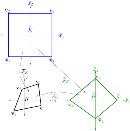
Figure 1: A bilinear map $\mathcal{F}_{K}$ from $\widehat{K}$ onto $K$, a bilinear map $\bar{\mathcal{F}}_{K}$ from $\widehat{K}$ onto $\bar{K}$, and an affine map $\bar{\mathcal{A}}_{K}$ from $\bar{K}$ onto $K$.

Define $\ell_{j},j=1,2$ by

$$\ell_{1}(\mathbf{x})=\frac{(\mathbf{x}-\mathbf{v}_{3})\times(\mathbf{v}_{1}-\mathbf{v}_{3})}{(\mathbf{v}_{2}-\mathbf{v}_{3})\times(\mathbf{v}_{1}-\mathbf{v}_{3})},\quad\ell_{2}(\mathbf{x})=\frac{(\mathbf{x}-\mathbf{v}_{4})\times(\mathbf{v}_{2}-\mathbf{v}_{4})}{(\mathbf{v}_{1}-\mathbf{v}_{4})\times(\mathbf{v}_{2}-\mathbf{v}_{4})},$$ (2.5)

where $\mathbf{a}\times\mathbf{b}$ denotes the cross product of vectors $\mathbf{a}$ and $\mathbf{b}.$ Then $\ell_{1}(\mathbf{x})=0$ and $\ell_{2}(\mathbf{x})=0$ are the equations of lines satisfying

$$\ell_{1}(\mathbf{v}_{1})=\ell_{1}(\mathbf{v}_{3})=0,\ell_{1}(\mathbf{v}_{2})=1;\,\ell_{2}(\mathbf{v}_{2})=\ell_{2}(\mathbf{v}_{4})=0,\ell_{2}(\mathbf{v}_{1})=1.$$ (2.6)

Then the intermediate quadrilateral $\bar{K}$ of MCL type is defined with the following four vertices:

$$\bar{\mathbf{v}}_{1}={1\choose 0},\bar{\mathbf{v}}_{2}={0\choose 1},\bar{\mathbf{v}}_{3}={\bar{h}_{1}\choose 0},\bar{\mathbf{v}}_{4}={0\choose\bar{h}_{2}},\text{ with }\bar{h}_{1}=\ell_{2}(\mathbf{v}_{3})<0,\bar{h}_{2}:=\ell_{1}(\mathbf{v}_{4})<0.$$ (2.7)

We will use $(x_{1},x_{2})$ and $(\bar{x}_{1},\bar{x}_{2})$ for the notations for coordinates in $K$ domain and $\bar{K}$ domain, respectively. The following proposition is useful for our analysis.

Proposition 2.4.

Let $\bar{\mathcal{A}}_{K}$ be an affine map defined by

$$\bar{\mathcal{A}}_{K}\bar{\mathbf{x}}=\begin{bmatrix}\bar{\mathcal{A}}_{K}^{(1)}&\bar{\mathcal{A}}_{K}^{(2)}\end{bmatrix}\bar{\mathbf{x}}+\boldsymbol{\xi},$$ (2.8)

where the three column vectors are defined by

$$\bar{\mathcal{A}}_{K}^{(1)}=\frac{\mathbf{v}_{1}-\mathbf{v}_{3}}{1-\bar{h}_{1}},\quad\bar{\mathcal{A}}_{K}^{(2)}=\frac{\mathbf{v}_{2}-\mathbf{v}_{4}}{1-\bar{h}_{2}},\quad\boldsymbol{\xi}=\frac{\mathbf{v}_{3}-\bar{h}_{1}\mathbf{v}_{1}}{1-\bar{h}_{1}}=\frac{\mathbf{v}_{4}-\bar{h}_{2}\mathbf{v}_{2}}{1-\bar{h}_{2}}.$$ (2.9)

Then $\bar{\mathcal{A}}_{K}:\mathbb{R}^{2}\to\mathbb{R}^{2}$ is an affine map which maps $\bar{K}$ onto $K.$ Moreover, the affine map $\bar{\mathcal{A}}_{K}^{-1}:K\to\bar{K}$ by

$${\bar{x}_{1}\choose\bar{x}_{2}}=\bar{\mathcal{A}}_{K}^{-1}\mathbf{x}={\ell_{2}(\mathbf{x})\choose\ell_{1}(\mathbf{x})}.$$ (2.10)

maps $K$ onto $\bar{K}$ with four corresponding vertices.

Proof.

Let $\boldsymbol{\xi}$ be the intersection of the line passing through $\mathbf{v}_{1}$ and $\mathbf{v}_{3}$ and the line passing through $\mathbf{v}_{2}$ and $\mathbf{v}_{4}.$ Then, we have

$$\bar{h}_{1}(\mathbf{v}_{1}-\boldsymbol{\xi})=(\mathbf{v}_{3}-\boldsymbol{\xi}),\quad\bar{h}_{2}(\mathbf{v}_{2}-\boldsymbol{\xi})=(\mathbf{v}_{4}-\boldsymbol{\xi}),$$ (2.11)

from which it follows that

$$\boldsymbol{\xi}=\frac{\mathbf{v}_{3}-\bar{h}_{1}\mathbf{v}_{1}}{1-\bar{h}_{1}}=\frac{\mathbf{v}_{4}-\bar{h}_{2}\mathbf{v}_{2}}{1-\bar{h}_{2}}.$$ (2.12)

Set $\bar{\mathcal{A}}_{K}^{(j)}=\mathbf{v}_{j}-\boldsymbol{\xi},j=1,2.$ Then, owing to (2.12), the column vectors and the shift vector $\boldsymbol{\xi}$ in (2.8) are given as in (2.9). It is immediate to verify that $\bar{\mathcal{A}}_{K}\bar{\mathbf{v}}_{j}=\mathbf{v}_{j},j=1,\cdots,4.$ ∎

Then the nonparametric MCL nonconforming quadrilateral element is defined as follows.

Definition 2.5 (Meng-Cui-Luo nonconforming quadrilateral element).

Define the intermediate reference element $(\bar{K},\bar{P}_{\bar{K}},\bar{\Sigma}_{\bar{K}})$ by (1) $\bar{K}$ is a typical quadrilateral of MCL type;    (2) $\bar{P}_{\bar{K}}^{npMCL}=P_{1}(\bar{K})\oplus\operatorname{Span}\{\bar{x}_{1}\bar{x}_{2}\};\quad$ (3) $\bar{\Sigma}^{npMCL}_{\bar{K}}=\{\sigma_{e}^{(i)},\,e\in\mathcal{E}(\bar{K})\}.$

Then the global nonparametric MCL nonconforming quadrilateral element space can be defined as follows:

$$\mathcal{NC}^{npMCL}_{h}=\{v\in L^{2}(\Omega)\,\mid\,v|_{K}=\bar{v}\circ\bar{A}_{K}^{-1}\text{ for some }\bar{v}\in\bar{P}^{npMCL}_{\bar{K}}\,\forall\,K\in\mathcal{T}_{h},$$

$$\hskip 227.62204pt\sigma_{e}^{(i)}(\left[\left[v\right]\right]_{e})=0\,\forall\,e\in\mathcal{E}^{i}_{h}\},$$

$$\mathcal{NC}^{npMCL}_{h,0}=\{v\in\mathcal{NC}^{npMCL}_{h}\,\mid\,\sigma_{e}^{i}(v)=0\,\forall\,~{}e\in\mathcal{E}_{h}^{b}\}.$$

Remark 2.6.

In [21] the polynomial space $P_{K}$ is defined as $P_{K}=\operatorname{Span}\{1,x_{1},x_{2},\ell_{1}(\mathbf{x})\ell_{2}(\mathbf{x})\}.$ But, due to the definitions of $\ell_{1},\ell_{2},$ and $\bar{\mathcal{A}}_{K},$ it is evident to see the two definitions of $P_{K}$ are identical.

Remark 2.7.

The Rannacher-Turek element is defined by using the reference element, and the basis function space $P_{K}$ in Definition 2.1 consists of $P_{1}(K)\oplus\operatorname{Span}\{\widehat{\phi}_{4}\circ\mathcal{F}_{K}^{-1}\},$ with $\widehat{\phi}_{4}(\widehat{\mathbf{x}})=\widehat{x}_{1}^{2}-\widehat{x}_{2}^{2}.$ Since the components of $\mathcal{F}_{K}^{-1}$ are not polynomials, the function $\widehat{\phi}_{4}\circ\mathcal{F}_{K}^{-1}(\mathbf{x})$ is not a polynomial. In contrast, the MCL finite element space $P_{K}$ in Definition 2.5 consists of quadratic polynomials since $\bar{\mathcal{A}}_{K}^{-1}(\mathbf{x})$ is an affine map.

Remark 2.8.

The convexity condition on $K$ is that

$$\bar{h}_{1}<0,\>\bar{h}_{2}<0.$$ (2.13)

3 Nonparametric DSSY elements in MCL-type domains

In this section, we use the intermediate domain $\bar{K}$ of MCL type to design a new nonconforming quadrilateral element with MVP.

Similarly to (2.3) as in [19], we aim to find a quartic polynomial $\bar{\mu}$ in $\bar{K}$ as follows:

$$\bar{\mu}(\bar{\mathbf{x}})=\bar{\ell}_{1}(\bar{\mathbf{x}})\bar{\ell}_{2}(\bar{\mathbf{x}})\bar{\mathscr{Q}}(\bar{\mathbf{x}}),$$ (3.1)

where ${\bar{\ell}}_{1}(\bar{\mathbf{x}})=\bar{x}_{2},\bar{\ell}_{2}(\bar{\mathbf{x}})=\bar{x}_{1},$ and $\bar{\mathscr{Q}}(\bar{\mathbf{x}})$ is a suitable quadratic polynomial. (Recall that the coordinate indices for $\bar{\ell}_{j}$ and $\bar{x}_{k}$ are switched as in (2.10).) We seek a quartic polynomial $\bar{\mu}(\bar{\mathbf{x}})$ fulfilling the MVP (2.2) in $\bar{K}$. Denote by $\bar{\mathbf{d}}_{j}:=\frac{\bar{\mathbf{v}}_{j+1}-\bar{\mathbf{v}}_{j}}{2}$ and $\bar{\mathbf{m}}_{j}$ the edge vector of $\bar{\mathbf{e}}_{j}$ and its midpoint for $j=1,\cdots,4$ (with indices modulo 4). An application of the three-point Gauss quadrature formula:

$$\int_{-1}^{1}f(t)~{}\operatorname{d}t\approx\frac{8}{9}f(0)+\frac{5}{9}(f(\xi)+f(-\xi)),\quad\xi=\sqrt{\frac{3}{5}},$$

which is exact for quartic polynomials, simplifies MVP (2.2) into the form

$$\bar{\mu}(\bar{\mathbf{g}}_{2j-1})+\bar{\mu}(\bar{\mathbf{g}}_{2j})-2\bar{\mu}(\bar{\mathbf{m}}_{j})=0,\quad j=1,\cdots,4,$$ (3.2)

where $\bar{\mathbf{g}}_{2j-1}=\bar{\mathbf{m}}_{j}-\xi\bar{\mathbf{d}}_{j},\quad\bar{\mathbf{g}}_{2j}=\bar{\mathbf{m}}_{j}+\xi\bar{\mathbf{d}}_{j},J=1,\cdots,4,$ together with $\bar{\mathbf{m}}_{j},j=1,\cdots,4,$ are the twelve Gauss points on the four edges. Notice that the equations of lines for edges $\bar{\mathbf{e}}_{j},j=1,\cdots,4,$ are given in vector notation as follows:

$$\bar{\mathbf{e}}_{j}(t)=\bar{\mathbf{m}}_{j}+t\bar{\mathbf{d}}_{j},\quad t\in[-1,1].$$

Consider the quartic polynomial (3.1) restricted to an edge $\bar{\mathbf{e}}_{j}(t),t\in[-1,1].$ Since $\bar{x}_{1}\bar{x}_{2}$ vanishes at the other two end points of each edge, one sees that

$$\bar{\ell}_{1}(\bar{\mathbf{g}}_{2j-1})\bar{\ell}_{2}(\bar{\mathbf{g}}_{2j-1})=\bar{\ell}_{1}(\bar{\mathbf{g}}_{2j})\bar{\ell}_{2}(\bar{\mathbf{g}}_{2j})=(1-\xi^{2})\bar{\ell}_{1}(\bar{\mathbf{m}}_{j})\bar{\ell}_{2}(\bar{\mathbf{m}}_{j}),\quad\left(\xi=\sqrt{\frac{3}{5}}\right).$$ (3.3)

A combination of (3.2) and (3.3) yields that (2.2) holds if and only if the quadratic polynomial $\bar{\mathscr{Q}}$ satisfies

$$\bar{\mathscr{Q}}(\bar{\mathbf{g}}_{2j-1})+\bar{\mathscr{Q}}(\bar{\mathbf{g}}_{2j})-5\bar{\mathscr{Q}}(\bar{\mathbf{m}}_{j})=0,\quad j=1,\cdots,4.$$ (3.4)

A standard use of symbolic calculation gives the general solution of (3.4) in the following one-parameter family in $\bar{c}$:

$$\bar{\mathscr{Q}}(\bar{\mathbf{x}})=\bar{q}(\bar{x}_{1};\bar{h}_{1})+\bar{c}\bar{q}(\bar{x}_{2};\bar{h}_{2}),\,\bar{c}\in\mathbb{R},\quad\text{where }\bar{q}(\bar{x};\bar{h})=\bar{x}^{2}-\frac{3}{10}(1+\bar{h})\bar{x}+\frac{3}{20}\bar{h}.$$ (3.5)

Define for each $\bar{c}\in\mathbb{R},$

$$\bar{\mu}(\bar{\mathbf{x}};\bar{c})=\bar{\ell}_{1}(\bar{\mathbf{x}})\bar{\ell}_{2}(\bar{\mathbf{x}})\bar{\mathscr{Q}}(\bar{\mathbf{x}})=\bar{x}_{1}\bar{x}_{2}\bar{\mathscr{Q}}(\bar{\mathbf{x}}).$$

where $\bar{\mathscr{Q}}$ by (3.5) depending on $\bar{c}$ as well as $\bar{\mathbf{x}}$.

We are now in a position to define a class of nonparametric nonconforming elements on the intermediate quadrilaterals $\bar{K}$ with four degrees of freedom as follows. (1) $\bar{K}=\mathcal{S}_{K}(\bar{K});\quad$ (2) $\bar{P}^{npDSSY}_{\bar{K}}=P_{1}(\bar{K})\oplus\operatorname{Span}\{\bar{\mu}(\bar{x}_{1},\bar{x}_{2};\bar{c})\}$ ; (3) $\bar{\Sigma}^{npDSSY}_{\bar{K}}=\{\sigma_{e}^{(i)},\,e\in\mathcal{E}(\bar{K})\}=\{\sigma_{e}^{(m)},\,e\in\mathcal{E}(\bar{K})\}.$

The global nonparametric DSSY quadrilateral nonconforming element spaces are defined similarly.

By the above construction it is apparent that MVP holds. Owing to this property, it is simple to show the unisolvency of the element.

Theorem 3.1.

Assume that $\bar{c}$ is chosen such that $\bar{h}_{1}^{2}+\bar{h}_{1}+1+\bar{c}(\bar{h}_{2}^{2}+\bar{h}_{2}+1)\neq 0.$ Then $(\bar{K},\bar{P}_{\bar{K}},\bar{\Sigma}_{\bar{K}})$ is unisolvent.

Proof.

Set $\bar{\psi}_{1}(\bar{\mathbf{x}})=1,\bar{\psi}_{2}(\bar{\mathbf{x}})=\bar{x}_{1},\bar{\psi}_{3}(\bar{\mathbf{x}})=\bar{x}_{2},$ and $\bar{\psi}_{4}=\bar{\mu}(\bar{x}_{1},\bar{x}_{2};\bar{c}),$ and define $A=(a_{jk})\in M_{4\times 4}(\mathbb{R})$ by $a_{jk}=\bar{\psi}_{k}(\bar{\mathbf{m}}_{j}),j,k=1,\cdots,4.$ Then, Using $\bar{q}(\frac{1}{2};\bar{h})=\frac{1}{10}$ and $\bar{q}(\frac{\bar{h}}{2};\bar{h})=\frac{\bar{h}^{2}}{10},$ we get

$$A=\begin{bmatrix}1&\frac{1}{2}&\frac{1}{2}&\frac{1}{40}(1+\bar{c})\\ 1&\frac{\bar{h}_{1}}{2}&\frac{1}{2}&\frac{1}{40}\bar{h}_{1}(\bar{h}_{1}^{2}+\bar{c})\\ 1&\frac{\bar{h}_{1}}{2}&\frac{\bar{h}_{2}}{2}&\frac{1}{40}\bar{h}_{1}\bar{h}_{2}(\bar{h}_{1}^{2}+\bar{c}\bar{h}_{2}^{2})\\ 1&\frac{1}{2}&\frac{\bar{h}_{2}}{2}&\frac{1}{40}\bar{h}_{2}(1+\bar{c}\bar{h}_{2}^{2})\end{bmatrix}$$ (3.6)

with $\det(A)=-\frac{1}{160}(1-\bar{h}_{1})^{2}(1-\bar{h}_{2})^{2}\big{(}\bar{h}_{1}^{2}+\bar{h}_{1}+1+\bar{c}(\bar{h}_{2}^{2}+\bar{h}_{2}+1)\big{)}.$ Thus $A$ is nonsingular if and only if $\bar{h}_{1}^{2}+\bar{h}_{1}+1+\bar{c}(\bar{h}_{2}^{2}+\bar{h}_{2}+1)\neq 0.$ ∎

From now on, we choose $\bar{c}=1$ to have symmetry in (3.5). The basis functions can be easily constructed by using MVP. For this, as in the proof of Theorem 3.1, set $\bar{\psi}_{1}(\bar{x})=1,\bar{\psi}_{2}(\bar{x})=\bar{x}_{1},\bar{\psi}_{3}(\bar{x})=\bar{x}_{2},\bar{\psi}_{4}(\bar{x})=\bar{\mu}(\bar{x},\bar{h})$ and seek the basis functions

$$\bar{\phi}_{j}(\bar{x})=\sum_{k=1}^{4}c_{jk}\bar{\psi}_{k}(\bar{x}),\,j=1,\cdots,4,\text{ such that }\bar{\phi}_{j}(\mathbf{m}_{k})=\delta_{jk}.$$ (3.7)

By computing the inverse of the matrix $A^{T}$ in (3.6), we can represent the basis functions (3.7) with the coefficients given by

$$(c_{jk})=\frac{2}{(1-\bar{h}_{1})(1-\bar{h}_{2})}\begin{bmatrix}\frac{\bar{h}_{1}\bar{h}_{2}}{2}&-\operatorname{N}(1,2)&-\operatorname{N}(2,1)&\frac{20}{\operatorname{D}}\\ -\frac{\bar{h}_{2}}{2}&\operatorname{N}(1,2)&\operatorname{Nh}(2)&-\frac{20}{\operatorname{D}}\\ \frac{1}{2}&-\operatorname{Nh}(1)&-\operatorname{Nh}(2)&\frac{20}{\operatorname{D}}\\ -\frac{\bar{h}_{1}}{2}&\operatorname{Nh}(1)&\operatorname{N}(2,1)&-\frac{40}{\operatorname{D}}\end{bmatrix},$$ (3.8)

where $\operatorname{D}=2+\bar{h}_{1}+\bar{h}_{2}+\bar{h}_{1}^{2}+\bar{h}_{2}^{2},\,\operatorname{N}(j,k)=\frac{(\bar{h}_{j}^{2}+\bar{h}_{j}+\bar{h}_{k}^{2}+1)\bar{h}_{k}}{\operatorname{D}},\,\operatorname{Nh}(j)=\frac{\bar{h}_{j}^{2}+\bar{h}_{j}+2}{\operatorname{D}},\,j,k=1,2.$

4 Effects of numerical integration

Consider the following elliptic boundary problem

$$-\nabla\cdot\left(\boldsymbol{\kappa}(x)\nabla\,u\right)&=f\text{ in }\Omega,\\ u=0\text{ on }\partial\Omega,$$ (4.1)

where $\Omega\subset\mathbb{R}^{n}$ is a polygonal domain and $\boldsymbol{\kappa}=\big{(}\boldsymbol{\kappa}_{ij}(x)\big{)}$ is a symmetric matrix with smooth functions $\boldsymbol{\kappa}_{ij}\in W^{1,\infty,h}(\Omega)$ such that there are constants $\alpha_{K}>0$ such that

$$\sum_{i,j=1}^{n}\kappa_{ij}(\mathbf{x})\xi_{i}\xi_{j}\geq\alpha_{K}|\xi|^{2},\,\mathbf{x}\in K\,\forall\,K\in\mathcal{T}_{h}.$$

The variational form of (4.1) is given by finding $u\in H_{0}^{1}(\Omega)$ such that

$$a(u,v)=F(v),\quad v\in H_{0}^{1}(\Omega),$$ (4.2)

where $a(u,v)=\int_{\Omega}\boldsymbol{\kappa}\nabla\,u\cdot\nabla\,vdx$ and $F(v)=\int_{\Omega}fvdx.$ Consider the nonparametric DSSY space $\mathcal{NC}^{npDSSY}_{h}$ defined by $(K,P_{K},\Sigma_{K})$ in the previous section. Then the finite element approximation $u_{h}\in\mathcal{NC}^{npDSSY}_{h}$ of (4.2) is defined as the solution of discrete problem

$$a_{h}(u_{h},v_{h})=F_{h}(v_{h}),\quad v\in\mathcal{NC}^{npDSSY}_{h}$$ (4.3)

where $a_{h}(u,v)=\sum_{K\in\mathcal{T}_{h}}\int_{K}\boldsymbol{\kappa}\nabla\,u\cdot\nabla\,vdx$ and $F_{h}(v)=\sum_{K\in\mathcal{T}_{h}}\int_{K}fvdx.$

The energy error estimate for nonconforming methods are as provided in [13].

Theorem 4.1.

[13] Assume that $u$ and $u_{h}$ are the solutions of (4.2) and (4.3), respectively. Then we have following error estimate

$$|u-u_{h}|_{1,h}\leq Ch|u|_{2,\Omega}.$$ (4.4)

Our aim in this section is to find sufficient conditions on numerical quadrature rules in approximating the stiffness matrix and load vector based on $\mathcal{NC}^{npDSSY}_{h}$. Notice that our nonconforming elements on $K$ are constructed via the affine map $\bar{\mathcal{A}}_{K}$ form the reference element $\bar{K}$ onto $K$. Thus it is natural to construct a quadrature formulae on $\bar{K}$, which is defined with positive weights $\bar{\omega}_{\bar{K},l}$ and nodes $\bar{\mathbf{b}}_{\bar{K},l}$, $l=1,\cdots,L,$ by

$$\int_{\bar{K}}\bar{\phi}(\bar{\mathbf{x}})d\bar{\mathbf{x}}\approx\sum_{l=1}^{L}\bar{\omega}_{\bar{K},l}\bar{\phi}({\bar{\mathbf{b}}}_{\bar{K},l}).$$ (4.5)

Denote by $J_{\bar{\mathcal{A}}_{K}}$ the Jacobian matrix of $\bar{\mathcal{A}}_{K}$, and observe that

$$\int_{K}\phi(\mathbf{x})d\mathbf{x}=|\det(J_{\bar{\mathcal{A}}_{K}})|\int_{\bar{K}}\bar{\phi}(\bar{\mathbf{x}})d\bar{\mathbf{x}}.$$

It induces the quadrature formulae on $K$ from (4.5), which is given by

$$\int_{K}\phi(\mathbf{x})d\mathbf{x}\approx\sum_{l=1}^{L}\omega_{K,l}\phi(\mathbf{b}_{K,l}),$$ (4.6)

where $\omega_{K,l}=|\det(J_{\bar{\mathcal{A}}_{K}})|\,\bar{\omega}_{\bar{K},l}$ and $\mathbf{b}_{K,l}=\bar{\mathcal{A}}_{K}\mathbf{\bar{b}}_{\bar{K},l}$. Suppose that the discrete problem (4.3) is approximated by above quadrature formulae. Then $\bar{u}_{h}$, the Galerkin approximation with quadrature, is defined as the solution of approximate problem: to find $\bar{u}_{h}\in\mathcal{NC}^{npDSSY}_{h}$ such that

$$\bar{a}_{h}(\bar{u}_{h},\bar{v}_{h})=\bar{F}_{h}({v}_{h}),\quad{v}_{h}\in\mathcal{NC}^{npDSSY}_{h},$$ (4.7)

where

$$\bar{a}_{h}(u,v)=\sum_{K\in\mathcal{T}_{h}}\omega_{K,l}(\boldsymbol{\kappa}\nabla\,u\cdot\nabla\,v)(\mathbf{b}_{K,l});\quad\bar{F}_{h}(v)=\sum_{K\in\mathcal{T}_{h}}\omega_{K,l}(fv)(\mathbf{b}_{K,l}).$$ (4.8)

Define the quadrature error functionals to estimate the effect of numerical integration by

$$\bar{E}_{\bar{K}}(\bar{\phi})&=\int_{\bar{K}}\bar{\phi}(\bar{\mathbf{x}})d\bar{\mathbf{x}}-\sum_{l=1}^{L}\bar{\omega}_{\bar{K},l}\phi(\mathbf{\bar{b}}_{\bar{K},l}),\\ E_{K}(\phi)=\int_{K}\phi(\mathbf{x})d\mathbf{x}-\sum_{l=1}^{L}\omega_{K,l}\phi(\mathbf{b}_{K,l}),$$ (4.9)

where above two error functionals are related as follows:

$$E_{K}(\phi)=|\det(J_{\bar{\mathcal{A}}_{K}})|\bar{E}_{\bar{K}}(\bar{\phi}).$$

The following Bramble-Hilbert Lemma is essential for our argument.

Lemma 4.2.

[10, Theorem 28.1, p.198] Let $D\subset\mathbb{R}^{n}$ be a domain with a Lipschitz continuous boundary. Suppose that $L$ is a continuous linear mapping on $W^{k+1,q}(D)$ for some integer $k\geq 0$ and $1\leq q\leq\infty$. If

$$L(\phi)=0\quad\forall\phi\in P_{k}(D),$$ (4.10)

then there exists a constant $C(D)$ such that

$$|L(v)|\leq C(D)\|L\|_{k+1,q,D}^{\prime}|v|_{k+1,q,D}\,\forall\,v\in W^{k+1,q}(D),$$ (4.11)

where $\|\cdot\|_{k+1,q,D}^{\prime}$ denotes the norm in the dual space of $W^{k+1,q}(D).$

The following theorem estimates the effect of quadrature formulae on the approximate bilinear form $\bar{a}_{h},$ whose proof is essentially identical to that of [10, Theorem 28.2, p.199].

Theorem 4.3.

Assume that $\bar{E}_{\bar{K}}(\bar{\phi})=0$ for any $\bar{\phi}\in\nabla\,\bar{P}_{\bar{K}}$, where

$$\nabla\,\bar{P}_{\bar{K}}:=\operatorname{Span}\{\nabla\,\bar{v}\;\big{|}\;\bar{v}\in\bar{P}_{\bar{K}}\}.$$

If $\boldsymbol{\kappa}\in W^{1,\infty}(K),$ then there exists a constant $C>0$ such that

$$\big{|}E_{K}(\boldsymbol{\kappa}\nabla\,u\cdot\nabla\,v)\big{|}\leq Ch_{K}||\boldsymbol{\kappa}||_{1,\infty,K}|u|_{1,K}|v|_{1,K}\quad\forall u,v\in P_{K},$$ (4.12)

where $h_{K}$ denotes the diameter of $K$.

We now establish the following conditional ellipticity estimate.

Theorem 4.4.

Assume that $\bar{E}_{\bar{K}}(\bar{\phi})=0$ for any $\bar{\phi}\in\nabla\,\bar{P}_{\bar{K}}$, where

$$\nabla\,\bar{P}_{\bar{K}}:=\operatorname{Span}\{\nabla\,\bar{v}\;\big{|}\;\bar{v}\in\bar{P}_{\bar{K}}\}.$$

Assume that $\boldsymbol{\kappa}\in W^{1,\infty}(\mathcal{T}_{h}).$ Then for sufficiently small $h>0$, the following ellipticity holds:

$$\bar{a}_{h}(v,v)\geq(\alpha-Ch|\kappa|_{1,\infty,h}){\color[rgb]{0,0,0}|v|_{1,h}^{2}}\,\forall\,v\in\mathcal{NC}^{npDSSY}_{h}.$$ (4.13)

Moreover, the conditional ellipticity coefficient in (4.13) can be given as $\min_{K\in\mathcal{T}_{h}}(\alpha_{K}-C_{K}h_{K}|\kappa|_{1,\infty,h}).$

Proof.

Let $v\in\mathcal{NC}^{npDSSY}_{h}$ be arbitrary. Then by the triangle inequality, the ellipticity, and Theorem 4.4, we have

$$\bar{a}_{h}(v,v)&\geq\sum_{K\in\mathcal{T}_{h}}\left[a_{K}(v,v)-|E_{K}(\kappa\nabla\,u,\nabla\,u)|\right]\\ \geq\min_{K\in\mathcal{T}_{h}}(\alpha_{K}-C_{K}h_{K}|\kappa|_{1,\infty,h}){\color[rgb]{0,0,0}|v|_{1,h}^{2}}\\ \geq(\alpha-Ch|\kappa|_{1,\infty,h}){\color[rgb]{0,0,0}|v|_{1,h}^{2}}.$$ (4.14)

This completes the proof. ∎

Next, we estimate the effect of numerical integration on the right hand side linear functional $\bar{F}_{h},$ which is essentially identical to the case of $k=1$ of [10, Theorem 28.3, p.201].

Theorem 4.5.

Suppose that $\bar{E}_{\bar{K}}(\bar{\phi})=0$ for any $\phi\in P_{0}(\bar{K})$. Then for arbitrary $f\in W^{1,\infty}(\Omega)$ and $\phi\in P_{K}$, there exists a constant $C>0$ such that

$$\big{|}E_{K}(f\phi)\big{|}\leq Ch_{K}|K|^{1/2}||f||_{1,\infty,K}||\phi||_{1,K}\,\forall\,\phi\in P_{K},$$

where $h_{K}$ denotes the diameter of $K$.

Finally, the effect of numerical integration is obtained by combining the above results.

Theorem 4.6.

Let $u$ and $\bar{u}_{h}$ be the solutions of (4.2) and (4.7), respectively. Assume that $\bar{E}_{\bar{K}}(\bar{\phi})=0$ for any $\bar{\phi}\in\nabla\,\bar{P}_{\bar{K}}.$ Assume that $\boldsymbol{\kappa}\in W^{1,\infty}(\mathcal{T}_{h}).$ Then, for sufficiently small $h>0,$ we have the following error estimate

$$|u-\bar{u}_{h}|_{1,h}\leq C\frac{h}{1-h\|\boldsymbol{\kappa}\|_{1,\infty,h}}\big{(}||\boldsymbol{\kappa}||_{1,\infty,h}|u|_{2,\Omega}+||f||_{1,\infty,h}\big{)}.$$

Proof.

We exploit the conditional uniform ellipticity of $\bar{a}_{h}$. Let $u_{h}$ be the solutions of (4.3). Then we have, for sufficiently small $h>0,$ for any $v_{h}\in\mathcal{NC}^{npDSSY}_{h}$,

$$(\alpha-Ch\|\boldsymbol{\kappa}\|_{1,\infty,h})|\bar{u}_{h}-v_{h}|_{1,h}^{2} \leq\bar{a}_{h}(\bar{u}_{h}-v_{h},\bar{u}_{h}-v_{h})$$

$$=\bar{a}_{h}(u_{h}-v_{h},\bar{u}_{h}-v_{h})+\bar{a}_{h}(\bar{u}_{h}-u_{h},\bar{u}_{h}-v_{h})$$

$$=\bar{a}_{h}(u_{h}-v_{h},\bar{u}_{h}-v_{h})+\big{(}\bar{F}_{h}(\bar{u}_{h}-v_{h})-\bar{a}_{h}(u_{h},\bar{u}_{h}-v_{h})\big{)}$$

$$=\bar{a}_{h}(u_{h}-v_{h},\bar{u}_{h}-v_{h})+\big{(}a_{h}(u_{h},\bar{u}_{h}-v_{h})-\bar{a}_{h}(u_{h},\bar{u}_{h}-v_{h})\big{)}$$

$$\qquad\qquad\qquad\qquad\qquad\,+\big{(}\bar{F}_{h}(\bar{u}_{h}-v_{h})-F_{h}(\bar{u}_{h}-v_{h})\big{)}.$$

Denote by $w_{h}:=\bar{u}_{h}-v_{h}$. It follows that

$$(\alpha-Ch\|\boldsymbol{\kappa}\|_{1,\infty,h})|\bar{u}_{h}-v_{h}|_{1,h} \leq C|u_{h}-v_{h}|_{1,h}+\frac{|a_{h}(u_{h},\bar{u}_{h}-v_{h})-\bar{a}_{h}(u_{h},\bar{u}_{h}-v_{h})|}{|\bar{u}_{h}-v_{h}|_{1,h}}$$

$$\quad\qquad\qquad\qquad+\frac{|F_{h}(\bar{u}_{h}-v_{h})-\bar{F}_{h}(\bar{u}_{h}-v_{h})|}{|\bar{u}_{h}-v_{h}|_{1,h}}$$

$$\leq C\inf_{v_{h}\in\mathcal{NC}^{npDSSY}_{h}}|u_{h}-v_{h}|_{1,h}$$

$$+\sup_{w_{h}\in\mathcal{NC}^{npDSSY}_{h}}\Big{(}\frac{|a_{h}(u_{h},w_{h})-\bar{a}_{h}(u_{h},w_{h})|}{|w_{h}|_{1,h}}+\frac{|\bar{F}_{h}(w_{h})-F_{h}(w_{h})|}{|w_{h}|_{1,h}}\Big{)}.$$

If we take $v_{h}=u_{h}$, the above inequality is simplified to

$$|\bar{u}_{h}-u_{h}|_{1,h} \leq\frac{1}{\alpha-Ch\|\boldsymbol{\kappa}\|_{1,\infty,h}}\sup_{w_{h}\in\mathcal{NC}^{npDSSY}_{h}}\Big{(}\frac{|a_{h}(u_{h},w_{h})-\bar{a}_{h}(u_{h},w_{h})|}{|w_{h}|_{1,h}}+\frac{|\bar{F}_{h}(w_{h})-F_{h}(w_{h})|}{|w_{h}|_{1,h}}\Big{)}.$$ (4.15)

It remains to estimate the above two consistency error terms. For the first term, using Theorem 4.3, we have

$$|a_{h}(u_{h},w_{h})-\bar{a}_{h}(u_{h},w_{h})| \leq\sum_{K\in\mathcal{T}_{h}}\big{|}E_{K}(\boldsymbol{\kappa}\nabla\,v_{h}\cdot\nabla\,w_{h})\big{|}$$

$$\leq\sum_{K\in\mathcal{T}_{h}}h_{K}||\boldsymbol{\kappa}||_{1,\infty,K}|v_{h}|_{1,K}|w_{h}|_{1,K}$$

$$\leq Ch||\boldsymbol{\kappa}||_{1,\infty,h}|u_{h}|_{1,h}|w_{h}|_{1,h}$$

$$\leq Ch||\boldsymbol{\kappa}||_{1,\infty,h}|u|_{2,\Omega}|w_{h}|_{1,h},$$ (4.16)

where the last inequality is obtained by the following estimate:

$$|u_{h}|_{1,h} \leq|u|_{1,\Omega}+|u-u_{h}|_{1,h}$$

$$\leq|u|_{1,\Omega}+Ch|u|_{2,\Omega}\leq C|u|_{2,\Omega}.$$

For the second consistency error term in (4.15), Theorem 4.5 applies:

$$|\bar{F}_{h}(w_{h})-F_{h}(w_{h})| \leq\sum_{K\in\mathcal{T}_{h}}\big{|}E_{K}(fw_{h})\big{|}$$

$$\leq C\sum_{K\in\mathcal{T}_{h}}h_{K}|K|^{1/2}||f||_{1,\infty,K}|w_{h}|_{1,K}$$

$$\leq Ch|\Omega|^{1/2}||f||_{1,\infty,h}|w_{h}|_{1,h}.$$ (4.17)

The theorem follows by combining (4.15)–(4) with the triangle inequality. That is, for sufficiently small $h>0,$

$$|u-\bar{u}_{h}|_{1,h} \leq|u-u_{h}|_{1,h}+|u_{h}-\bar{u}_{h}|_{1,h}$$

$$\leq Ch|u|_{2,\Omega}+C\frac{h}{1-h\|\boldsymbol{\kappa}\|_{1,\infty,h}}\big{(}||\boldsymbol{\kappa}||_{1,\infty,h}|u|_{2,\Omega}+|\Omega|^{1/2}||f||_{1,\infty,h}\big{)}$$

$$\leq C\frac{h}{1-h\|\boldsymbol{\kappa}\|_{1,\infty,h}}\big{(}||\boldsymbol{\kappa}||_{1,\infty,h}|u|_{2,\Omega}+||f||_{1,\infty,h}\big{)}.$$

∎

5 Construction of quadrature formulae

In this section we construct quadrature formulae for the nonparametric DSSY element defined in Section 3.

5.1 Quadrature formula on $\bar{K}$

In [21], the basis functions are at most of degree two so that the quadrature formulae of degree two is found. However our element has high-order degree polynomial basis to fulfill MVP, and thus we require some other quadrature formulae. Following the analysis of previous section, we may find quadrature formulae exact for functions in $\bar{\mathcal{Q}}$, which is defined as

$$\bar{\mathcal{Q}}:=\operatorname{Span}\{\nabla\,\bar{u}\;\big{|}\;\bar{u},\bar{v}\in\bar{P}_{\bar{K}}\}=\operatorname{Span}\{1,\frac{\partial\bar{\mu}}{\partial\bar{x}_{1}},\frac{\partial\bar{\mu}}{\partial\bar{x}_{2}}\}$$

to preserve the order of convergence. From now on, we choose $\bar{c}=1,$ the generalization being trivial to include the other cases.

We quote the formula from [21, (1) p.330]:

$$\int_{\bar{K}}\bar{x}_{1}^{j}\bar{x}_{2}^{k}d\bar{\mathbf{x}}=\sum_{k=1}^{4}\int_{\bar{T}_{k}}\bar{x}_{1}^{j}\bar{x}_{2}^{k}d\bar{\mathbf{x}}=\frac{j!k!}{(2+j+k)!}(1-{\bar{h}_{1}}^{j+1})(1-{\bar{h}_{2}}^{k+1}).$$ (5.1)

We have the area

$$|\bar{K}|=\frac{(1-\bar{h}_{1})(1-\bar{h}_{2})}{2}.$$

For the sake of notational simplicity, we write

$$\bar{\bar{h}}_{1}:=1+\bar{h}_{1},\quad\bar{\bar{h}}_{2}:=1+\bar{h}_{2},\quad\bar{\bar{h}}_{1}<1,\,\bar{\bar{h}}_{2}<1.$$

Clearly, $\bar{\bar{\mathbf{h}}}_{c}=\frac{1}{3}{\bar{\bar{h}}_{1}\choose\bar{\bar{h}}_{2}}$ is the barycenter of $\bar{K}.$

5.2 One-point quadrature rule of precision 1

The obvious one-point quadrature weight and point are given by

$$\bar{\omega}_{1}=|\bar{K}|,\quad\bar{\boldsymbol{\xi}}^{(1)}=\bar{\bar{\mathbf{h}}}_{c}.$$ (5.2)

5.3 Two-point and three-point quadrature rules of precision 1

We seek two-point and three-point quadrature rules (4.5) with equal weights at one stroke. The weights are then given by $\omega_{\bar{K},l}=\frac{|K|}{L},l=1,\cdots,L,$ for $L=2,3.$ The Gauss points $\mathbf{\bar{b}}_{\bar{K},l},l=1,\cdots,L,$ are assumed to be geometrically symmetric with respect to the barycenter $\bar{\bar{\mathbf{h}}}_{c}.$ Hence we seek $\boldsymbol{\xi}^{(L)}={\xi_{1}^{(L)}\choose\xi_{2}^{(L)}}$ such that

$$\int_{\bar{K}}\bar{\phi}(\bar{\mathbf{x}})d\bar{\mathbf{x}}\approx\begin{cases}\frac{|K|}{2}\left(\bar{\phi}(\bar{\bar{\mathbf{h}}}_{c}+\boldsymbol{\xi}^{(2)})+\bar{\phi}(\bar{\bar{\mathbf{h}}}_{c}-\boldsymbol{\xi}^{(2)})\right)&\text{for }L=2,\\ \frac{|K|}{3}\left(\bar{\phi}(\bar{\bar{\mathbf{h}}}_{c})+\bar{\phi}(\bar{\bar{\mathbf{h}}}_{c}+\boldsymbol{\xi}^{(3)})+\bar{\phi}(\bar{\bar{\mathbf{h}}}_{c}-\boldsymbol{\xi}^{(3)})\right)&\text{for }L=3,\end{cases}$$ (5.3)

which are exact for

$$\frac{\partial\bar{\mu}}{\partial\bar{x}_{1}}&=3\bar{x}_{1}^{2}\bar{x}_{2}+\bar{x}_{2}^{3}-\frac{3}{10}(2\bar{\bar{h}}_{1}\bar{x}_{1}\bar{x}_{2}+\bar{\bar{h}}_{2}\bar{x}_{2}^{2})+\frac{3}{20}(\bar{\bar{h}}_{1}+\bar{\bar{h}}_{2}-2)\bar{x}_{2},\\ \frac{\partial\bar{\mu}}{\partial\bar{x}_{2}}=\bar{x}_{1}^{3}+3\bar{x}_{1}\bar{x}_{2}^{2}-\frac{3}{10}(\bar{\bar{h}}_{1}\bar{x}_{1}^{2}+2\bar{\bar{h}}_{2}\bar{x}_{1}\bar{x}_{2})+\frac{3}{20}(\bar{\bar{h}}_{1}+\bar{\bar{h}}_{2}-2)\bar{x}_{1}.$$ (5.4)

Then, by utilizing (5.1), the exactness of (5.3) for (5.4) implies that $(\xi^{(L)}_{1},\xi^{(L}_{2}),L=2,3,$ turn out to be the solutions $(X,Y)$ of the quadratic equations:

$$10\bar{\bar{h}}_{2}X^{2}+14\bar{\bar{h}}_{1}XY+7\bar{\bar{h}}_{2}Y^{2}&=Lr(\bar{\bar{h}}_{1},\bar{\bar{h}}_{2}),\\ 7\bar{\bar{h}}_{1}X^{2}+14\bar{\bar{h}}_{2}XY+10\bar{\bar{h}}_{1}Y^{2}=Lr(\bar{\bar{h}}_{2},\bar{\bar{h}}_{1}),$$ (5.5)

where $r(u,v)=\frac{5}{4}v\left(\frac{2}{90}u^{2}-\frac{4}{10}u+\frac{185}{999}v^{2}-\frac{6}{10}v+1\right).$ Since (5.5) is a symmetric system of homogeneous quadratic equations, it is easy to see the following lemma.

Lemma 5.1.

The four solutions of (5.5) are given by $\pm(g_{1}(\bar{\bar{h}}_{1},\bar{\bar{h}}_{2}),g_{1}(\bar{\bar{h}}_{2},\bar{\bar{h}}_{1})),$ and
$\pm(g_{2}(\bar{\bar{h}}_{1},\bar{\bar{h}}_{2}),g_{2}(\bar{\bar{h}}_{2},\bar{\bar{h}}_{1}))$ for some functions $g_{1}(u,v)$ and $g_{2}(u,v).$

Denote by $r_{1}$ and $r_{2}$ the right hand sides of (5.5). Then a judicial use of symbolic software (for example, Julia or Matlab) with some cook-ups gives the following two pairs of solutions $(X,Y)$:

$$X^{(1)}(\bar{\bar{h}}_{1},\bar{\bar{h}}_{2})&=-\frac{T_{4}+\sqrt{T_{3}}}{T_{1}}Y^{(1)}(\bar{\bar{h}}_{1},\bar{\bar{h}}_{2}),\quad Y^{(1)}(\bar{\bar{h}}_{1},\bar{\bar{h}}_{2})=\sqrt{\frac{T_{5}+T_{6}\sqrt{T_{3}}}{T_{2}}};\\ X^{(2)}(\bar{\bar{h}}_{1},\bar{\bar{h}}_{2})=-\frac{T_{4}-\sqrt{T_{3}}}{T_{1}}Y^{(2)}(\bar{\bar{h}}_{1},\bar{\bar{h}}_{2}),\quad Y^{(2)}(\bar{\bar{h}}_{1},\bar{\bar{h}}_{2})=\sqrt{\frac{T_{5}-T_{6}\sqrt{T_{3}}}{T_{2}}},$$ (5.6)

where $T_{1}=7r_{1}\bar{\bar{h}}_{1}-10r_{2}\bar{\bar{h}}_{2},\,T_{2}=13720\bar{\bar{h}}_{1}^{4}-26603\bar{\bar{h}}_{1}^{2}\bar{\bar{h}}_{2}^{2}+13720\bar{\bar{h}}_{2}^{4},\,T_{3}=-70(r_{1}^{2}\bar{\bar{h}}_{1}^{2}+r_{2}^{2}\bar{\bar{h}}_{2}^{2})+49(r_{1}^{2}\bar{\bar{h}}_{2}^{2}+r_{2}^{2}\bar{\bar{h}}_{1}^{2})+51r_{1}r_{2}\bar{\bar{h}}_{1}\bar{\bar{h}}_{2},\,T_{4}=7(r_{1}\bar{\bar{h}}_{2}-r_{2}\bar{\bar{h}}_{1}),\,T_{5}=-1043r_{1}\bar{\bar{h}}_{1}^{2}\bar{\bar{h}}_{2}+980r_{1}\bar{\bar{h}}_{2}^{3}+686r_{2}\bar{\bar{h}}_{1}^{3}-470r_{2}\bar{\bar{h}}_{1}\bar{\bar{h}}_{2}^{2},\,T_{6}=14(7\bar{\bar{h}}_{1}^{2}-10\bar{\bar{h}}_{2}^{2}).$ Owing to the symmetries of $T_{2}$ and $T_{3}$ with respect to $\bar{\bar{h}}_{1}$ and $\bar{\bar{h}}_{2}$, one can check by using symbolic software, again, that $X^{(j)}(\bar{\bar{h}}_{1},\bar{\bar{h}}_{2})=Y^{(j)}(\bar{\bar{h}}_{2},\bar{\bar{h}}_{1}),j=1,2,$ which confirms Lemma 5.1. Obviously, $T_{2}>0$ unless $\bar{\bar{h}}_{1}=0$ and $\bar{\bar{h}}_{2}=0.$ Among the two pairs of solutions $(X^{(j)},Y^{(j)}),j=1,2,$ in (5.6), we choose one that is closer to the origin $(0,0)$ if $\bar{\bar{\mathbf{h}}}_{c}+{X^{(j)}\choose Y^{(j)}}$ is in $\bar{K}$ to increase numerical stability.

In the case where $\bar{\bar{h}}_{1}=0$ or $\bar{\bar{h}}_{2}=0,$ $T_{1}$ vanishes, and therefore, the above formula is unstable. To deal with this, first, assume the case of $\bar{\bar{h}}_{2}=0.$ Then, the polynomial equations corresponding to (5.5) are simplified as follows:

$$1008\bar{\bar{h}}_{1}(2-\bar{\bar{h}}_{1})XY&=0,\\ 252X^{2}+360Y^{2}=25\bar{\bar{h}}_{1}^{2}-81\bar{\bar{h}}_{1}+135.$$ (5.7)

From (5.7) and (5.7), we have either (i) $X^{(1)}=0,Y^{(1)}=\sqrt{\frac{25\bar{\bar{h}}_{1}^{2}-81\bar{\bar{h}}_{1}^{2}+135}{360}}$ or (ii) $Y^{(2)}=0,X^{(2)}=\sqrt{\frac{25\bar{\bar{h}}_{1}^{2}-81\bar{\bar{h}}_{1}^{2}+135}{252}}.$ Among these two pair $(X^{(j)},Y^{(j)}),j=1,2,$ the suitable choice is made as above.

The case of $\bar{\bar{h}}_{1}=0$ is treated similarly by rotation of the case of $\bar{\bar{h}}_{2}=0.$

6 Numerical examples

In this section some numerical results are reported to confirm the theoretical parts about the quadrature developed in the previous sections.

Example 6.1.

For the numerical example, consider the elliptic boundary value problem (4.1) on $\Omega=(0,1)^{2}$ and $\kappa(\textbf{x})=1+(1+x_{1})(1+x_{2})+\epsilon\sin(10\pi x_{1})\sin(5\pi x_{2}).$ The source term $f$ is generated by the exact solution

$$u(x_{1},x_{2})=\sin(3\pi x_{1})x_{2}(1-x_{2})+\epsilon\sin\left(\frac{\pi x_{1}}{\epsilon}\right)\sin\left(\frac{\pi x_{2}}{\epsilon}\right),\quad\epsilon=0.2.$$

The above problem is solved by using the nonparametric DSSY element constructed in Section 3. Let $\bar{u}_{h}$ denote the nonparametric DSSY Galerkin approximation to $u$ by using any specific Gauss quadrature rule (4.7). The meshes used in the numerical example are perturbed from $(N\times N)$ uniform rectangles as follows. The random meshes $x_{jk},j,k=1,\cdots,N-1,$ are obtained by perturbing the uniform mesh points $(j,k)h,h=\frac{1}{N}$ with randomly by $r_{1}$ and $r_{2}$ such that $x_{jk}=(j+r_{jk,1},k+r_{jk,2})h$ with $|r_{jk,l}|\leq r,l=1,2.$ Here, $r=0.2$ was chosen. The linear systems are solved by the Conjugate Gradient method with tolerance $10^{-7}$ for residuals. The errors and reduction ratios with random perturbation are averaged with 20 ensembles, but the number of ensembles can be arbitrarily increased. Our 2–point and 3–point Gauss quadrature rules are compared with the standard $2\times 2$–point and $3\times 3$–point tensor product Gauss quadrature rules in computing the stiffness matrix and the right hand side vectors. In order to make the comparison fair to the above four different quadrature rules, all errors are calculated by using $3\times 3$–point tensor product Gauss quadrature.

$N$	$2\times 2$ Gauss quadrature				$3\times 3$ Gauss quadrature
	$|\bar{u}_{h}-u|_{1,h}$	order	$\|\bar{u}_{h}-u\|_{0}$	order	$|\bar{u}_{h}-u|_{1,h}$	order	$\|\bar{u}_{h}-u\|_{0}$	order
4	4.37		0.213		2.45		0.131
8	4.17	0.688E-01	0.857E-01	1.31	1.72	0.508	0.426E-01	1.62
16	2.39	0.803	0.240E-01	1.84	0.926	0.896	0.112E-01	1.92
32	1.29	0.888	0.661E-02	1.86	0.471	0.975	0.286E-02	1.97
64	0.731	0.821	0.204E-02	1.69	0.237	0.994	0.718E-03	1.99
128	0.476	0.619	0.825E-03	1.31	0.118	0.998	0.180E-03	2.00
256	0.384	0.311	0.497E-03	0.732	0.592E-01	0.999	0.450E-04	2.00

Table 1: Numerical results of Example 6.1 on random meshes with tensor product Gauss quadratures: the broken $H^{1}(\Omega)$–seminorm and $L^{2}(\Omega)$–norm errors and their reduction orders are reported.

$N$	$2$–pt Gauss quadrature				$3$–pt Gauss quadrature
	$|\bar{u}_{h}-u|_{1,h}$	order	$\|\bar{u}_{h}-u\|_{0}$	order	$|u-\bar{u}_{h}|_{1,h}$	order	$\|\bar{u}_{h}-u\|_{0}$	order
4	13.2		0.960		4.61		0.539
8	9.04	0.548	0.228	2.08	2.42	0.927	0.113	2.26
16	4.15	1.12	0.457E-01	2.32	1.15	1.08	0.208E-01	2.44
32	2.10	0.984	0.107E-01	2.09	0.559	1.04	0.388E-02	2.42
64	1.06	0.979	0.263E-02	2.03	0.279	1.00	0.835E-03	2.21
128	0.533	0.999	0.655E-03	2.01	0.139	1.00	0.200E-03	2.06
256	0.267	0.999	0.163E-03	2.00	0.698E-01	0.997	0.494E-04	2.02

Table 2: Numerical results of Example 6.1 on random meshes with 2-pt and 3-pt Gauss quadratures: the broken $H^{1}(\Omega)$–seminorm and $L^{2}(\Omega)$–norm errors and their reduction orders are reported.

As seen from the tables, the $2\times 2$ tensor product Gauss quadrature is not sufficient to integrate the matrices in the nonparametric DSSY element methods, while the $3\times 3$ tensor product rule is sufficient. In the meanwhile, our new 2–pt Gauss quadrature rule is almost optimal, which gives better numerical results than the $2\times 2$ product rule. Observe that numerical errors obtained by our $3$–pt Gauss quadrature rule are as good as those obtained by using the $3\times 3$ tensor product rule. In most calculations, the 2–pt Gauss quadrature rule is acceptable.

References

• [1] B. Achchab, A. Agouzal, and K. Bouihat. A simple nonconforming quadrilateral finite element. C. R. Acad. Sci. Paris, Ser. I., 352(6):529–533, 2014.
• [2] B. Achchab, A. Agouzal, and K. Bouihat. A new class of nonconforming finite elements for arbitrary order. Rendiconti Sem. Mat. Univ. Pol. Torino, 76(2):11–17, 2018.
• [3] R. Altmann and C. Carstensen. $P_{1}$-nonconforming finite elements on triangulations into triangles and quadrilaterals. SIAM J. Numer. Anal., 50(2):418–438, 2012.
• [4] T. Arbogast and Z. Chen. On the implementation of mixed methods as nonconforming methods for second-order elliptic problems. Math. Comp., 64(211):943–972, 1995.
• [5] I. Babuška, U. Banerjee, and H. Li. The effect of numerical integration on the finite element approximation of linear functionals. Numer. Math., 117(1):65–88, 2011.
• [6] U. Banerjee and J. E. Osborn. Estimation of the effect of numerical integration in finite element eigenvalue approximation. Numer. Math., 56(8):735–762, 1989.
• [7] U. Banerjee and M. Suri. The effect of numerical quadrature in the $p$-version of the finite element method. Math. Comp., 59(199):1–20, 1992.
• [8] Z. Cai, J. Douglas, Jr., J. E. Santos, D. Sheen, and X. Ye. Nonconforming quadrilateral finite elements: A correction. Calcolo, 37(4):253–254, 2000.
• [9] Z. Cai, J. Douglas, Jr., and X. Ye. A stable nonconforming quadrilateral finite element method for the stationary Stokes and Navier-Stokes equations. Calcolo, 36:215–232, 1999.
• [10] P. Ciarlet. Basic error estimates for elliptic problems. In Finite Element Methods (Part 1), volume II of Handbook of Numerical Analysis, pages 17–351. North Holland, Amsterdam, 1991.
• [11] P. G. Ciarlet and P.-A. Raviart. The combined effect of curved boundaries and numerical integration in isoparametric finite element methods. In The mathematical foundations of the finite element method with applications to partial differential equations, pages 409–474. Elsevier, 1972.
• [12] M. Crouzeix and P. Raviart. Conforming and nonconforming finite element methods for solving the stationary Stokes equations. I. R.A.I.R.O.– Math. Model. Anal. Numer., 7(R-3):33–75, 1973.
• [13] J. Douglas, Jr., J. E. Santos, D. Sheen, and X. Ye. Nonconforming Galerkin methods based on quadrilateral elements for second order elliptic problems. ESAIM–Math. Model. Numer. Anal., 33(4):747–770, 1999.
• [14] M. Fortin. A three-dimensional quadratic nonconforming element. Numer. Math., 46:269–279, 1985.
• [15] M. Fortin and M. Soulie. A non-conforming piecewise quadratic finite element on the triangle. Int. J. Numer. Meth. Engrg., 19(4):505–520, 1983.
• [16] H. Han. Nonconforming elements in the mixed finite element method. J. Comp. Math., 2:223–233, 1984.
• [17] R. Herbold, M. Schultz, and R. Varga. The effect of quadrature errors in the numerical solution of boundary value problems by variational techniques. aequationes mathematicae, 3(3):247–270, 1969.
• [18] R. Herbold and R. Varga. The effect of quadrature errors in the numerical solution of two-dimensional boundary value problems by variational techniques. aequationes mathematicae, 7(1):36–58, 1971.
• [19] Y. Jeon, H. Nam, D. Sheen, and K. Shim. A class of nonparametric DSSY nonconforming quadrilateral elements. ESAIM: Mathematical Modelling and Numerical Analysis, 47(6):1783–1796, 2013.
• [20] A. Linke, G. Matthies, and L. Tobiska. Robust arbitrary order mixed finite element methods for the incompressible Stokes equations with pressure independent velocity errors. ESAIM: Mathematical Modelling and Numerical Analysis, 50(1):289–309, 2016.
• [21] Z. Meng, J. Cui, and Z. Luo. A new rotated nonconforming quadrilateral element. Journal of Scientific Computing, 74(1):324–335, 2018.
• [22] H. E. Osborn and U. Banerjee. Estimation of the effect of numerical integration in finite element eigenvalue approximation. Numer. Math., 56:735–762, 1990.
• [23] C. Park and D. Sheen. $P_{1}$-nonconforming quadrilateral finite element methods for second-order elliptic problems. SIAM J. Numer. Anal., 41(2):624–640, 2003.
• [24] R. Rannacher and S. Turek. Simple nonconforming quadrilateral Stokes element. Numer. Methods Partial Differential Equations, 8:97–111, 1992.
• [25] A. H. Stroud and D. Secrest. Gaussian Quadrature Formulas. Prentice–Hall, Englewood Cliffs, NJ, 1966.
• [26] S. Turek. Efficient solvers for incompressible flow problems, volume 6 of Lecture Notes in Computational Science and Engineering. Springer, Berlin, 1999.
• [27] H. Zeng, C.-S. Zhang, and S. Zhang. Optimal quadratic element on rectangular grids for $H^{1}$ problems. BIT Numerical Mathematics, pages 1–25, 2020.
• [28] X. Zhou, Z. Meng, and Z. Luo. New nonconforming finite elements on arbitrary convex quadrilateral meshes. Journal of Computational and Applied Mathematics, 296:798–814, 2016.