Approximate Solutions of a Kinetic Theory for Graphene

Abstract

The effective mass approximation is analysed in a nonperturbative kinetic theory approach to strong field excitations in graphene  [1, 2]. This problem is highly actual for the investigation of quantum radiation from graphene [3], where the collision integrals in the photon kinetic equation are rather complicated functionals of the distribution functions of the charge carriers. These functions are needed in the explicit analytical definition as solutions of the kinetic equations for the electron-hole excitations. In the present work it is shown that the suggested approach is rather effective in a certain range of parameters for the pulse of an external electromagnetic field. For example, the applicability condition of the approximation in the case of a harmonic field is $\hbar\omega^{2}/(\sqrt{2}eE_{0}v_{F})<1,$ were $v_{F}$ is the Fermi velocity. In the standard massive quantum electrodynamics the usability of the analogical approximation is very narrow.

1 Introduction

It is well known that the interaction of carriers in graphene with with an external electromagnetic field is nonanalytic in the coupling constant [4, 5]. This renders applications of perturbation theory unjustified and stimulates the search for nonperturbative approaches. Paradigms are here exactly solvable quantum field theory models [6, 7]. However, these solutions are limited to narrow classes of external field models (constant electric field, Eckart’s potential). Alternative cases are founded either on direct application of the basic equations of motion [8, 9] or on the nonperturbative kinetic theory [1, 2, 3, 10] constructed in analogy to the standard strong field QED [11, 12, 13, 14].

A higher level of description of the graphene excitations is connected with the investigation of different mechanisms of radiation. In the simplest case the question is about the emission of a quasiclassical electromagnetic field by the plasma currents in graphene [15, 16]. There is also the radiation of a quantized field that is the result of the direct interaction of the charge carriers with the photon field. A consistent realization of this approach is based on a truncation procedure of the Bogoliubov-Born-Green-Kirkwood-Yvon (BBGKY) chain of equations for the correlation functions of the $eh\gamma$ – system [3]. This leads to a closed system of kinetic equations (KEs) with collision integrals (CIs) of non-Markovian type in the electron-hole and photon sectors and with the Maxwell equation for the acting inner (plasma) field. As far as the evolution of the $eh$-plasma is accompanied by high-frequency quantum (vacuum, as in the case of the electron - positron plasma) oscillations, any solution of this KE system turns out very susceptible to the selection not only of the model and the parameters of the external field but also to the necessary roughening in the process of calculating the physical quantities.

Below we will consider this problem on the examples of two approximative methods for the solution of the basic KEs describing the production of $eh$-pairs under the action of an external field: the low density approximation [17] and the method of the asymptotic decompositions [18] (Sect. 2). The ideas for these approaches are borrowed from the standard QED. In the considered case of the massless theory, an essential role plays the effective mass approximation [19]. The results of analytical calculations of the basic functions of the kinetic theory are compared among themselves and with the exactly solvable model (Sect. 3). The considered examples show that the introduction of the effective electromagnetic mass allows to obtain rather simple expansions for the distribution functions of the $eh$-plasma in graphene for time dependent electric fields with different pulse shape.

2 The basic KE and its approximate solutions

The basic KE for description of excitation and evolution of the $eh$-plasma in graphene under the action of an external quasiclassical spatially uniform time-dependent electric field with the vector potential $A^{\mu}=(0,A^{(1)}(t),A^{(2)}(t),0)$ in the Hamiltonian gauge $A^{(0)}=0$ can be written in the integro-differential form [1, 2, 3, 10]

$$\dot{f}(\mathbf{p},t)=\frac{1}{2}\lambda(\mathbf{p},t)\int_{t_{0}}^{t}\lambda(\mathbf{p},t^{\prime})[1-2f(\mathbf{p},t^{\prime})]\cos\theta(\mathbf{p};t,t^{\prime})dt^{\prime}$$ (1)

or as the equivalent system of ordinary differential equations

$$\dot{f}(\mathbf{p},t)=\frac{1}{2}\lambda(\mathbf{p},t)u(\mathbf{p},t),$$ (2)

$$\dot{u}(\mathbf{p},t)=\lambda(\mathbf{p},t)\left[1-2f(\mathbf{p},t)\right]-\frac{2\varepsilon(\mathbf{p},t)}{\hbar}\nu(\mathbf{p},t),\ \dot{\nu}(\mathbf{p},t)=\frac{2\varepsilon(\mathbf{p},t)}{\hbar}u(\mathbf{p},t).$$

Here $f(\mathbf{p},t)$ is the distribution function of charge carriers introduced by taking into account the electroneutrality $f(\mathbf{p},t)=f_{e}(\mathbf{p},t)=f_{h}(-\mathbf{p},t)$. The excitation function $\lambda(\mathbf{p},t)$ in the low energy model is determined as

$$\lambda(\mathbf{p},t)=\frac{ev_{F}^{2}[E^{(1)}(t)P^{2}-E^{(2)}(t)P^{1}]}{\varepsilon^{2}(\mathbf{p},t)},$$ (3)

where $v_{F}=10^{6}\$ m/s is the Fermi velocity, $E^{(k)}=-\frac{1}{c}\dot{A}^{(k)}(t)$ is the field strength $(k=1,2)$, $P^{k}=p^{k}+\frac{e}{c}A^{k}(t)$ is the quasi-momentum and $\varepsilon(\mathbf{p},t)=v_{F}\sqrt{P^{2}}$ is the quasi-energy. The electron charge is $-e$. Finally, the quantity $\theta(\mathbf{p};t,t^{\prime})$ in the KE (1) is the phase,

$$\theta(\mathbf{p};t,t^{\prime})=\frac{2}{\hbar}\int_{t^{\prime}}^{t}dt^{\prime\prime}\varepsilon(\mathbf{p},t^{\prime\prime}).$$ (4)

The KE (1) is an integro-differential equation of the non-Markovian type with a fastly oscillating kernel. There is an integral of motion

$$(1-2f)^{2}+u^{2}+v^{2}={\rm const},$$ (5)

where the constant is fixed with the corresponding initial condition.

The KEs (1), (2) for the case of graphene were obtained in the works [1, 2, 3, 10] by the Bogoliubov method of canonical transformations that can by realized in the massless $D=2+1$ theory in an explicit form. On the other hand the system (2) can be reduced from the general system of twelve KEs in the standard QED [20].

The massless low energy model of graphene with the lightlike dispersion law $\varepsilon(\mathbf{p},t)$ leads to the absence of the critical field that is characteristic for massive QED and results in a specific feature of the momentum dependence of the excitation function $\lambda(\mathbf{p},t)$ (3): this function decreases in the ultraviolet area, $\lambda(\mathbf{p},t)\sim 1/P\rightarrow 0$ at $P\rightarrow\infty$ and is singular in the infra-red area $\lambda(\mathbf{p},t)\rightarrow\infty$ at $P\rightarrow 0$. The last distinction also leads to a nonanalytic structure of the theory in its dependence on the coupling constant and to the absence of the standard perturbation theory.

Let us write also the differential equation of the third order that is equivalent to the system of equations (2),

$$\stackrel{{\scriptstyle...}}{{g}}+\ddot{g}\left[\varepsilon\lambda\left(\frac{1}{\varepsilon\lambda}\right)^{\prime}-\frac{\dot{\lambda}}{\lambda}\right]+\dot{g}\left[4\varepsilon^{2}+\lambda^{2}-\varepsilon\lambda\left(\frac{\dot{\lambda}}{\varepsilon\lambda^{2}}\right)^{\prime}\right]+g\varepsilon\lambda\left(\frac{\lambda}{\varepsilon}\right)^{\prime}=0,$$ (6)

where $g=1-2f$. In Eq. (6) the ^′ denotes also the time derivative.

At the present time, an exact solution of the KEs (1), (2) is not known. However, below we will assume that the well-known exact solutions of the Dirac equation for a constant electric field and the Eckart potential are at the same time solutions of the KEs (1), (2). This assumption gives a basis for comparing these exact solutions with the known approximate solutions of the KEs (1), (2) and to construct then some new classes of approximate solutions.

In order to estimate the effectivity of the approximate solutions, we will compare them to the exact solutions (analytical and numerical). Such a comparison will be made on the level of an integral macroscopic quantity. The number density of pairs $n(t)$ will be considered as the simplest quantity of such type,

$$n(t)=\frac{N_{f}}{(2\pi\hbar)^{2}}\int f(\mathbf{p},t)d\mathbf{p},$$ (7)

where $N_{f}=4$ is the number of flavours. The integration allows here to smoothen out some insignificant details in the momentum dependence of the distribution functions in different approximations.

As the next step, we will consider two approximate methods of solving the KEs (1), (2). To this end, we will consider the case of a linearly polarized electric field $A^{(1)}=0,\ A^{(2)}(t)=A(t)$.

2.1 Low density approximation

This approximation corresponds to the limit $f\ll 1$ in the r.h.s. KE (1). It was introduced in the strong field vacuum production of charged particles [17] and was used many times in strong field QED and in the kinetic theory of excitations in graphene. It leads to the quadrature formula [1, 2]

$$f(t)=\frac{1}{4}\left[\int_{-\infty}^{t}dt^{\prime}\lambda_{s}(t^{\prime})\right]^{2}+\frac{1}{4}\left[\int_{-\infty}^{t}dt^{\prime}\lambda_{c}(t^{\prime})\right]^{2},$$ (8)

where

$$\lambda_{c}(t)=\lambda(t)\cos\theta(t,-\infty),\ \ \lambda_{s}(t)=\lambda(t)\sin\theta(t,-\infty).$$ (9)

In particular, it follows from Eq. (8), that $f(\mathbf{p},t)\geq 0$.

In the low-density approximation, the two last KEs of the system (2) separate from it,

$$\dot{u}=\lambda-\frac{2\varepsilon}{\hbar}v,\ \dot{v}=\frac{2\varepsilon}{\hbar}u.$$ (10)

Then the distribution function $f$ can be found from the first equation of the system (2) alone.

The system of equations (10) corresponds to the ordinary differential equation,

$$\frac{\hbar}{2\varepsilon}\frac{d}{dt}\left(\frac{\hbar}{2\varepsilon}\frac{du}{dt}\right)+u-\frac{\hbar}{2\varepsilon}\frac{d}{dt}\left(\frac{\hbar\lambda}{2\varepsilon}\right)=0$$ (11)

or

$${\cal D}^{2}u+u-{\cal D}\left(\frac{\hbar\lambda}{2\varepsilon}\right)=0,\ {\cal D}=\frac{\hbar}{2\varepsilon}\frac{d}{dt}.$$ (12)

2.2 Effective electromagnetic mass approximation

This approximation was used already in the case of the harmonic model of an external field in the analysis of the radiation effects in the $e^{-}e^{+}$ plasma [21] and in the $eh$ plasma in graphene [3]. Below we will consider a generalization of this approach to other models of the external field.

The idea of the method is that the time dependent value of the square of the kinetic momentum $P^{2}(t)$ in the definition of the quasienergy $\varepsilon(\mathbf{p},t)$ gets substituted by corresponding time average $\prec P^{2}(t)\succ$, where the symbol $\prec...\succ$ means the averaging procedure over a characteristic time of the external field. In the case of the linearly polarized electric field we obtain

$$\prec P^{2}_{2}(t)\succ=p^{2}_{2}+(e/c)^{2}\prec A^{2}(t)\succ,$$ (13)

if $\prec A(t)\succ=0$. Implying the substitution

$$P^{2}_{2}(t)\rightarrow\prec P^{2}_{2}(t)\succ,$$ (14)

in the square of quasienergy $\varepsilon^{2}(\mathbf{p},t)=v^{2}_{F}[p^{2}_{1}+P^{2}_{2}(t)]$, one can introduce the longitudinal (with respect to external field) effective electromagnetic mass

$$(e/c)^{2}\prec A^{2}(t)\succ=m^{2}_{\ast}v^{2}_{F},$$ (15)

or

$$m_{\ast}^{2}=\frac{e^{2}}{c^{2}v_{F}^{2}}\frac{1}{2T}\int_{-T}^{T}dtA^{2}(t).$$ (16)

Thus, this approximation corresponds to change

$$\varepsilon(\mathbf{p},t)\rightarrow\varepsilon_{\ast}(\mathbf{p})=v_{F}\sqrt{p_{1}^{2}+(p_{2}^{2}+m^{2}_{\ast}v^{2}_{F})}.$$ (17)

The appearance of the longitudinal mass is a reflection of the anisotropy of the system stipulated by the presence of the external field and leads to a reduction of the mobility of charge carriers along the direction of the action of the external field. In the limiting case $p_{2}\ll m_{\ast}v_{F}$, we obtain a strong anisotropic momentum dependence of the quasienergy,

$$\varepsilon_{\ast}(\mathbf{p})=v_{F}\sqrt{m^{2}_{\ast}v^{2}_{F}+p_{1}^{2}}.$$ (18)

The approximation of the effective mass (14), (15) is valid in field models with square integrable functions $A(t)$ only.

The transition amplitude (3) in the effective mass approximation in the linearly polarized external field will be

$$\lambda_{\ast}(\mathbf{p},t)=-\frac{ev^{2}_{F}p_{1}}{\varepsilon^{2}_{\ast}(\mathbf{p})}E(t)\equiv\Lambda(\mathbf{p})E(t),$$ (19)

where $p_{1}=\cos\varphi$ and $\varphi$ is the polar angle.

The problem of evaluating the distribution function is now brought to the calculation of the integral

$$J(\mathbf{p},t)=\int_{-\infty}^{t}dt^{\prime}E(t^{\prime})\cos\theta_{\ast}(\mathbf{p};t^{\prime},-\infty),$$ (20)

where $\theta_{\ast}(\mathbf{p};t^{\prime},-\infty)$ is defined by the relation (4) with the replacement $\varepsilon(\mathbf{p},t)\rightarrow\varepsilon_{\ast}(\mathbf{p})$. The analogous integral with the replacement $\cos\theta_{\ast}\rightarrow\sin\theta_{\ast}$ is equal to zero, if $E(t)=E(-t)$. The distribution function (8) will then be

$$f(\mathbf{p},t)=\frac{1}{4}\Lambda^{2}(\mathbf{p})J^{2}(\mathbf{p},t).$$ (21)

According to the relations (19) and (21), the anisotropy of the distribution function $\sim\cos^{2}\varphi$ is universal and does not depend on the selection of the external field model. Another distinctive feature of the amplitude (19) is the singular slit of the surfaces $\lambda(\mathbf{p},t)$ on the plane $(p_{1},p_{2})$ along the axis $p_{1}=0$ (or $\varphi=\pi/2$) for $p_{2}\neq 0$, i.e. $\lambda(\mathbf{p},t)|_{p_{1}=0}=0,$ and $\lambda(\mathbf{p},t)|_{p_{1}\neq 0}\neq 0$. As it follows from the KEs (1) and (2), this peculiarity is reproduced also in the distribution function, $f(\mathbf{p},t)|_{p_{1}=0}=0$. This means that quasiparticles are not created in the directions of the external field action in the strict sense. Fig. 1 demonstrates this on the example of the Sauter impulse. This slit is evident in the figures shown below in the case of the massless version of the theory. The introduction of a mass results in a widening of this slit and in the appearance of the energy gap. Let us remark, that the exact solution of the problem [7] in the case of the Sauter pulse field has the singular line $p_{1}=0$ in the case of the linearly polarized external field. The presence of this infinitely thin slit is not reflected in calculations of the integral ”observable” macroscopical averages of the type of the pair number density (7).

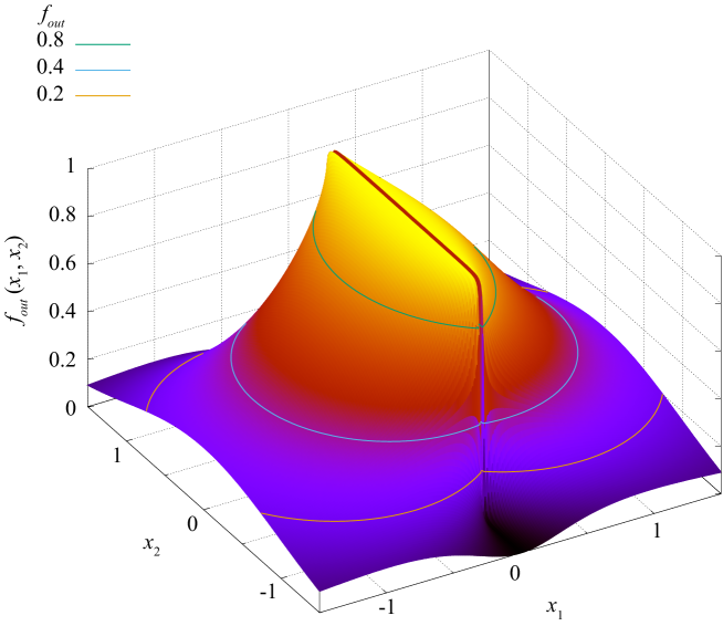
Figure 1: The residual distribution function $f_{out}(x_{1},x_{2})$ for the Sauter field model with $E=1000\ {\rm V/cm},\kappa=10^{12}\ {\rm Hz}$, where $x_{1,2}=p_{1,2}/m_{\ast}v_{F}$ are dimensionless momenta.

2.3 Method of asymptotic decompositions

This method is adopted from the standard strong field QED [18]. We consider now the dimensionless excitation amplitude in the exact case (3)

$$\Lambda(\mathbf{p},t)=e\hbar v^{2}_{F}E(t)p^{1}/2\varepsilon^{3}(\mathbf{p},t)$$ (22)

and in the effective mass approximation

$$\Lambda_{\ast}(\mathbf{p},t)=e\hbar v^{2}_{F}E(t)p^{1}/2\varepsilon^{3}_{\ast}(\mathbf{p},t).$$ (23)

In contrast to $\Lambda(\mathbf{p},t)$, the amplitude $\Lambda_{\ast}(\mathbf{p},t)$ (23) is limited everywhere,

$$\Lambda_{\ast}(\mathbf{p},t)\leq\Lambda_{\ast}^{max}=\frac{e\hbar E_{0}}{3\sqrt{3}m^{2}_{\ast}v^{3}_{F}},$$ (24)

where $\Lambda_{\ast}^{max}$ is the maximal value of the amplitude (23) in the point of time where $E(t)=E_{0}$ (see Fig.1).

In order to clarify the physical meaning of the parameter $\Lambda_{\ast}^{max}$ given in (24), let us consider the case of a harmonic field, where the momentum of the electromagnetic field is equal to $p_{A}=(e/c)A(t)\sim eE_{0}/\omega$. It corresponds to the contribution of the electromagnetic field in the quasienergy $\varepsilon_{A}=v_{F}p_{A}=eE_{0}v_{F}/\omega$. Then the relation (24) can be rewritten as

$$\Lambda_{\ast}^{max}=\frac{2\hbar\omega^{2}}{3\sqrt{3}eE_{0}v_{F}}\sim\frac{\hbar\omega}{\varepsilon_{A}},$$ (25)

which corresponds to the ratio of the energy of the absorbed quant of external field to the part of energy of quasiparticle acquired as a result of acceleration in this field.

In the case of a sufficiently large low-frequency external field, $\hbar\omega\ll eE_{0}v_{F}$, one can search a solution of the KE system (2) by means of an asymptotic decomposition of the functions $f,\ u,\ v$ for the small parameter $\Lambda_{\ast}(\mathbf{p},t)\ll\Lambda_{\ast}^{max}\ll 1$,

$$f=\sum_{n=0}f_{n},\quad u=\sum_{n=0}u_{n},\quad v=\sum_{n=0}v_{n}.$$ (26)

Substituting these decompositions in the KE system (2) and equating the contributions of the same orders, one can obtain the leading terms of the asymptotic decompositions (26) as

$$f_{4} = \frac{1}{4}\Lambda^{2}_{\ast}(\mathbf{p},t)=\frac{e^{2}v^{4}_{F}E^{2}(t)p_{1}^{2}}{16\varepsilon^{6}_{\ast}},$$ (27)

$$u_{3} = \frac{1}{2\varepsilon_{\ast}}\dot{\Lambda}_{\ast}(\mathbf{p},t)=\frac{ev^{2}_{F}\dot{E}(t)p_{1}}{4\varepsilon^{4}_{\ast}},\quad v_{2}=\Lambda_{\ast}(\mathbf{p},t).$$

Formally, these expressions have the same form as the analogous results in standard QED which were obtained in the framework of the asymptotic decompositions of the functional series in $E_{0}/E_{c}\ll 1$, where $E_{c}=m^{2}c^{3}/e\hbar$ is the critical field. In a similar way one can obtain the post-leading terms.

The obtained asymptotic solutions of the KE (2) can be used for estimating the convergences of the integral macroscopical physical values (e.g., the densities of the conduction and polarization currents an so on) and also in analytical calculations in theory of radiation and other transport phenomena.

Let us consider now the realization of the effective mass approximation for different external field models.

3 Approximate solutions of KEs for different external field models in graphene

3.1 The Sauter pulse

The field of this pulse is given by

$$A(t)=-(cE_{0}/\kappa)\tanh\kappa t,\ E(t)=E_{0}/\cosh^{2}\kappa t~{}.$$ (28)

It is a classical example of the external field model leading to an exact solution of the basic equations of motion of QED [11]. The analogous solution for the massless graphene model was obtained in the work [7].

The effective electromagnetic mass (16) in this model is

$$m_{\ast}=eE_{0}/v_{F}\kappa.$$ (29)

The corresponding integral (20) is

$$J(\mathbf{p},t)=\frac{E_{0}}{\kappa}\int_{-\infty}^{\kappa t}dx\frac{\cos[\Omega(\mathbf{p})/\kappa]x}{\cosh^{2}x},$$ (30)

where $\Omega(\mathbf{p})=2\varepsilon_{\ast}(\mathbf{p})/\hbar$. The corresponding distribution function $f(\mathbf{p},t)$ is defined then according to the Eq. (21). The vacuum polarization functions $u(\mathbf{p},t)$ and $v(\mathbf{p},t)$ can be restored then with help of the Eqs. (2). In the asymptotic limit $t\rightarrow\infty$ it follows that

$$J_{out}(\mathbf{p})=\frac{2E_{0}}{\kappa}\frac{\pi\Omega(\mathbf{p})/2\kappa}{\sinh[\pi\Omega(\mathbf{p})/2\kappa]}.$$ (31)

Then the distribution function (21) in the out-state will be

$$f_{out}(\mathbf{p})=\left[\frac{eE_{0}v^{2}_{F}p_{1}}{\kappa\varepsilon^{2}_{\ast}(\mathbf{p})}\frac{\pi\Omega(\mathbf{p})/2\kappa}{\sinh[\pi\Omega(\mathbf{p})/2\kappa]}\right]^{2}.$$ (32)

The corresponding expression for the pair number density (7) written in terms of the dimensionless momentum $x_{k}=p_{k}/m_{\ast}v_{F}$ is

$$n_{out}=\frac{N_{f}}{\pi}\left(\frac{\eta^{2}\kappa}{8\pi v_{F}}\right)^{2}\int_{0}^{\infty}\frac{dx\ x^{3}}{1+x^{2}}\frac{1}{\left[\sinh\left(\frac{\eta}{2}\sqrt{1+x^{2}}\right)\right]^{2}},$$ (33)

where

$$\eta=\frac{2\pi m_{\ast}v^{2}_{F}}{\hbar\kappa}=\frac{2\pi eE_{0}v_{F}}{\hbar\kappa^{2}}.$$ (34)

The point $\eta=1$ separates two domains: the domain $\eta<1$, where the energy of quasiparticles acquired in the external field per unit of time $eE_{0}v_{F}/\kappa$ is less than the energy of an absorbed quant of the field $\hbar\kappa$, and the domain $\eta>1$, where the field acceleration mechanism dominates.

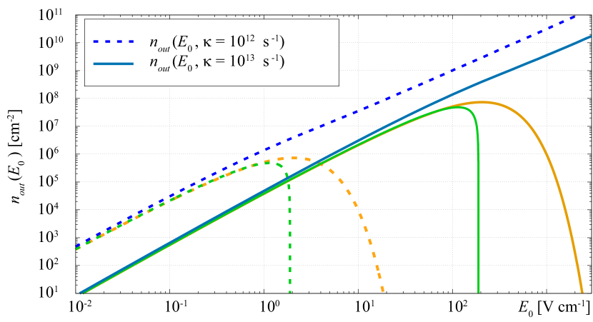
Figure 2: Sauter field model for two values $\kappa=10^{12}\ {\rm s}^{-1}$ and $\kappa=10^{13}\ {\rm s}^{-1}$. Blue lines are numerical solutions of KE (1), orange lines are approximate solutions (33), green lines are approximate solutions (35).

Some results of the numerical comparison of the exact and approximate (34) dependencies $n_{out}(\eta)$ are given in Fig. 2. From here it follows that the effective electromagnetic mass approximation is valid in the domain $\eta\leq 1$ and can be dubbed ”slow switching” with $\kappa\gg(2\pi eE_{0}v_{F}/\hbar)^{1/2}$. Assuming that $\eta\ll 1$ on the r.h.s. of Eq. (33), one can obtain

$$n_{out}=-\frac{N_{f}}{\pi}\left(\frac{eE_{0}}{2\hbar\kappa}\right)^{2}\left[1+\frac{1}{2}\ln\frac{1}{24}+\ln\eta\right],\quad\eta\ll 1.$$ (35)

This corresponds to the result obtained in [7].

3.2 The Gaussian pulse

This field model

$$A(t)=-\sqrt{\frac{\pi}{2}}cE_{0}\tau{\rm erf}\left(\frac{t}{\sqrt{2}\tau}\right),\ E(t)=E_{0}\exp(-t^{2}/2\tau^{2})$$ (36)

results in the effective mass

$$m_{\ast} = \frac{eE_{0}\tau\pi^{1/4}}{v_{F}}\left(\sqrt{2}\ {\rm erf}(1/\sqrt{2})e^{-1/2}+\sqrt{\pi}\ {\rm erf}^{2}(1/\sqrt{2})/2-{\rm erf}(1)\right)^{1/2}$$ (37)

$$\sim 0.5257\ \frac{eE_{0}\tau}{v_{F}}.$$

The distribution function will be

$$f(\mathbf{p},t)=\frac{1}{2}\left[\frac{eE_{0}v^{2}_{F}\tau p_{1}}{\varepsilon^{2}_{\ast}(\mathbf{p})}\ I\left(\frac{t}{\sqrt{2}\tau},\sigma\right)\right]^{2},$$ (38)

where $\sigma=\Omega(\mathbf{p})\tau$ and

$$I\left(\frac{t}{\sqrt{2}\tau},\sigma\right)=\int_{0}^{t/\sqrt{2}\tau}dx\cos(\sqrt{2}\sigma x)e^{-x^{2}}.$$ (39)

A simple result follows from Eq. (38) and (39) in the asymptotic case $t\rightarrow\infty$,

$$f_{out}(\mathbf{p})=\frac{\pi}{2}\left\{\frac{eE_{0}\tau v_{F}^{2}p_{1}}{\varepsilon^{2}_{\ast}(\mathbf{p})}\exp\left[-\frac{2\varepsilon^{2}_{\ast}\tau^{2}}{\hbar^{2}}\right]\right\}^{2}.$$ (40)

From here one can find after simple calculations the pair number density in the out-state,

$$n_{out}=-N_{f}\left(\frac{e\tau E_{0}}{4\hbar}\right)^{2}\left[e^{-\xi^{2}}+(1+\xi^{2}){\rm Ei}(-\xi^{2})\right],$$ (41)

where $\xi=2m_{\ast}v^{2}_{F}\tau/\hbar$ and ${\rm Ei}(-\xi^{2})$ is the exponential integral function. This result in the region $\xi\ll 1$ corresponds to Eq. (35) for the case of the Sauter pulse.

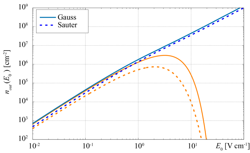
Figure 3: The pair number densities $n_{out}$ for the numerical (blue lines) and approximate (orange lines) solutions for the Sauter ($\kappa=10^{12}\ \rm{s}^{-1}$) and Gauss ($\tau=10^{-12}\ \rm{s}$) pulses.

In Fig. 3 we compare the behaviour of the pair number densities $n_{out}$ for the exact and approximate solutions for the Sauter ($\kappa=10^{12}\ \rm{s}^{-1}$) and Gauss ($\tau=10^{-12}\ \rm{s}$) pulses.

3.3 The harmonic field model

The harmonic field model

$$A(t)=-(cE_{0}/\omega)\sin\omega t,\ E(t)=E_{0}\cos\omega t;$$ (42)

corresponds to the effective mass

$$m_{\ast}=eE_{0}/\sqrt{2}v_{F}\omega.$$ (43)

The distribution function in this field model was obtained in the work [3],

$$f(\mathbf{p},t)=f^{(0)}(\mathbf{p})+f^{(2)}(\mathbf{p},t),$$ (44)

where the function

$$f^{(0)}(\mathbf{p})=\frac{(e\hbar E_{0}v_{F}^{2}p_{1})^{2}(4\varepsilon_{\ast}^{2}+\hbar^{2}\omega^{2})}{8\varepsilon_{\ast}^{4}(4\varepsilon_{\ast}^{2}-\hbar^{2}\omega^{2})^{2}}$$ (45)

corresponds to a stationary background distribution while the function

$$f^{(2)}(\mathbf{p},t)=\frac{(e\hbar E_{0}v_{F}^{2}p_{1})^{2}}{8\varepsilon_{\ast}^{4}(4\varepsilon_{\ast}^{2}-\hbar^{2}\omega^{2})}\cos 2\omega t$$ (46)

corresponds to the breathing mode on the doubled frequency of the external field. The residual functions $u,\ v$ can be reconstructed using Eqs. (44)-(46) and the KE system (2)

$$u(\mathbf{p},t)=\frac{e\hbar^{2}v_{F}^{2}p_{1}}{\varepsilon_{\ast}^{2}(4\varepsilon_{\ast}^{2}-\hbar^{2}\omega^{2})}\dot{E}(t),$$ (47)

$$v(\mathbf{p},t)=\frac{2e\hbar^{2}v_{F}^{4}p_{1}}{\varepsilon_{\ast}(4\varepsilon_{\ast}^{2}-\hbar^{2}\omega^{2})}E(t).$$ (48)

The distribution function (44)-(45) corresponds to the first and third harmonics of the current density and radiation spectrum of the plasma oscillations [3]. These results are valid in the case

$$\hbar\omega^{2}/(\sqrt{2}eE_{0}v_{F})<1.$$ (49)

This limitation holds also for other field models, if the quantity $\omega$ is interpreted as the corresponding characteristic frequency of the field alteration.

A general feature of the two outlined approximate approaches is the $E^{2}$ - proportionality of all the resulting distribution functions, $f(\mathbf{p},t)\sim(eE_{0})^{2}$. This feature was obtained in the work [22] on the basis of an analysis of the numerical solutions of the corresponding KEs in standard QED, see also [23].

The effectiveness of the low density approximation in the standard strong field QED for rather weak fields $E_{0}\ll E_{c}$ has been investigated in the work [24]. The additional introduction of the effective mass approximation results herein a strong restriction of the domain of applicability of the method.

4 Conclusion

In the present work we have obtained some simple and rather universal results of approximate solutions for the distribution functions of charge carriers in graphene based on nonperturbative KEs. This was achieved by a combination of the low density approximation and the concept of an effective electromagnetic mass. Such an approach is effective for a rather wide classes of external field models with the parameters limited by the relation for the top (49) of the characteristic frequency $\omega$ of the external field.

The considered approximation is of particular interest for the investigation of such complicated nonlinear single-photon effects in graphene as the emission (absorption) and annihilation (photoproduction) [3] and the more complex two-photon processes. Such kind of nonlinear phenomena in graphene became accessible for experimental verification recently, see [15, 16].

Acknowledgements

The work of D.B. was supported by the Russian Federal Program ”Priority-2030”. N.G. received support from Volkswagen Foundation (Hannover, Germany) under collaborative research grant No. 97029. B.M. acknowledges a stipend from the International Max Planck Research School for ”Many-Particle Systems in Structured Environments” at the Max-Planck Institute for Physics of Complex Systems (Dresden, Germany).

References

- [1] Smolyansky, S.A., Panferov, A., Blaschke, D., Gevorgayn, N.: Nonperturbative Kinetic Description of Electron-Hole Excitations in Graphene in a Time Dependent Electric Field of Arbitrary Polarization. Particles 2, 208–230 (2019). \doi10.3390/particles2020015
- [2] Smolyansky, S.A., Panferov, A.D., Blaschke, D.B., Gevorgyan, N.T.: Kinetic Equation Approach to Graphene in Strong External Fields. Particles 3(2), 456–476 (2020). \doi10.3390/particles3020032
- [3] Gavrilov, S.P., Gitman, D.M., Dmitriev, V.V., Panferov, A.D., Smolyansky, S.A.: Radiation Problems Accompanying Carrier Production by an Electric Field in the Graphene. Universe 6, 205 (2020). \doi10.3390/universe6110205
- [4] Vozmediano, M.A.H., Katsnelson, M.I., Guinea, F.: Gauge fields in graphene. Phys. Rep. 496, 109–148 (2010). \doi10.1016/j.physrep.2010.07.003
- [5] Lewkowicz, M., Kao, H.C., Rosenstein, B.: Signature of the Schwinger pair creation rate via radiation generated in graphene by a strong electric current. Phys. Rev. B 84, 035414 (2011). \doi10.1103/PhysRevB.84.035414
- [6] Gavrilov, S.P., Gitman, D.M., Yokomizo, N.: Dirac fermions in strong electric field and quantum transport in graphene. Phys. Rev. D 86, 125022 (2012). \doi10.1103/PhysRevD.86.125022
- [7] Klimchitskaya, G.L., Mostepanenko, V.M.: Creation of quasiparticles in graphene by a time-dependent electric field. Phys. Rev. D 87, 125011 (2013). \doidoi:10.1103/PhysRevD.87.125011
- [8] Ishikava, K.L.: Nonlinear optical response of graphene in time domain. Phys. Rev. B 82, 201402 (2010). \doi10.1103/PhysRevB.82.201402
- [9] Ishikava, K.L.: Electronic response of graphene to an ultrashort intense terahertz radiation pulse. New J.of Phys. 15, 055021 (2013). \doi10.1088/1367-2630/15/5/055021
- [10] Panferov, A.D., Churochkin, D.V., Fedotov, A.M., Smolyansky, S.A., Blaschke, D.B., Gevorgyan, N.T.: Nonperturbative kinetic description of e-h excitations in graphene due to a strong, time-dependent electric field. In Proceedings of the Ginzburg Centennial Conference on Physics, May 29 - June 3, 2017, Moscow. http://gc2.lpi.ru/proceedings/panferov.pdf Last accessed 16 March 2020
- [11] Grib A.A., Mamaev, S.G., Mostepanenko, V.M.: Vacuum Quantum Effects in Strong Fields. Friedmann Laboratory Publishing, St.Petersburg, Russia, (1994)
- [12] Bialynicky-Birula, I., Gornicki, P., Rafelski, J.: Phase space structure of the Dirac vacuum. Phys. Rev. D 44, 1825 (1991). \doi10.1103/PhysRevD.44.1825
- [13] Schmidt, S.M., Blaschke, D., Röpke, G., Smolyansky, S.A., Prozorkevich, A.V., Toneev, V.D.: A Quantum kinetic equation for particle production in the Schwinger mechanism. Int. J. Mod. Phys. E 7, 709–718 (1998). \doi10.1142/S0218301398000403
- [14] Kluger, Y., Mottola, E., Eisenberg, J.: Quantum Vlasov equation and its Markov limit. Phys. Rev. D 58, 125015 (1998). \doi10.1103/PhysRevD.58.125015
- [15] Bowlan, P., Martinez-Moreno, E., Reimann, K., Elsaesser, T., Woerner, M.: Ultrafast terahertz response of multilayer graphene in the nonperturbative regime. Phys. Rev. B. 89, 041408 (2014). \doi10.1103/PhysRevB.89.041408
- [16] Baudisch, M., Marini, A., Cox, J.D. et al.: Ultrafast nonlinear optical response of Dirac fermions in graphene. Nat Commun 9, 1018 (2018). \doi10.1038/s41467-018-03413-7
- [17] Schmidt, S. M., Blaschke, D., Röpke, G., Prozorkevich, A. V., Smolyansky, S. A., Toneev, V. D.: Non-Markovian effects in strong-field pair creation. Phys. Rev. D 59, 094005 (1999). \doi10.1103/PhysRevD.59.094005
- [18] Mamaev, S. G., Trunov, N. N.: Vacuum polarization and particle production in a non-stationary homogeneous electromagnetic field. Sov. J. Nucl. Phys. 30, 677 (1979)
- [19] Berestetskii, V. B., Lifshitz, E. M., Pitaevskii, L. P.: Quantum Electrodynamics. Pergamon, Oxford (1982)
- [20] Aleksandrov, I. A., Dmitriev, V. V., Sevostyanov, D. G., Smolyansky, S. A.: Kinetic description of vacuum e+e- production in strong electric fields of arbitrary polarization. Eur. Phys. J. Spec. Top. 229, 3469-3485 (2020). \doi10.1140/epjst/e2020-000056-1
- [21] Smolyansky, S. A., Fedotov, A. M.; Dmitriev, V. V.: Kinetics of the vacuum e-e+ plasma in a strong electric field and problem of radiation. Mod. Phys. Lett. A 35, 2040028 (2020). \doi10.1142/S0217732320400283
- [22] Kravtcov, K. Y., Dmitriev, V. V., Levenets, S. A., Panfyorov, A. D., Smolyansky, S. A., Juchnowski, L., Blaschke, D. B.: The choice of the optimal approximation in the kinetic description of the vacuum creation of electron-positron plasma in strong laser fields. In: Derbov, V. L., Postnov, D.E. (eds.) SARATOV FALL MEETING 2017, Laser Physics and Photonics XVIII; and Computational Biophysics and Analysis of Biomedical Data IV, vol. 10717, p. 1071702 (2018). \doi10.1117/12.2306171
- [23] Blaschke, D. B., Juchnowski L., Otto, A.: Kinetic Approach to Pair Production in Strong Fields—Two Lessons for Applications to Heavy-Ion Collisions. Particles 2, no.2, 166-179 (2019). \doi10.3390/particles2020012
- [24] Fedotov, A. M., Gelfer, E. G., Korolev, K. Yu., Smolyansky, S. A.: On the kinetic equation approach to pair production by time-dependent electric field. Phys. Rev D 83, 025011 (2011). \doi10.1103/PhysRevD.83.025011