Constraining IGM enrichment and metallicity with the C IV forest correlation function

Abstract

The production and distribution of metals in the diffuse intergalactic medium (IGM) have implications for galaxy formation models, cosmic star formation history, and the baryon (re)cycling process. Furthermore, the relative abundance of metals in high versus low-ionization states has been argued to be sensitive to the Universe’s reionization history. However, measurements of the background metallicity of the IGM at $z\sim 4$ are sparse and in poor agreement with one another, and reduced sensitivity in the near-IR implies that probing IGM metals at $z>4$ is currently out of reach if one adheres to the traditional method of detecting individual absorbers. We present a new technique based on clustering analysis that enables the detection of these weak IGM absorbers by statistically averaging over all spectral pixels, here applied to the C iv forest. We simulate the $z=4.5$ IGM with different models of inhomogeneous metal distributions whereby halos above a minimum mass enrich their environments with a constant metallicity out to a maximum radius. We generate mock skewers of the C iv forest and investigate its two-point correlation function (2PCF) as a probe of IGM metallicity and enrichment topology. The 2PCF of the C iv forest demonstrates a clear peak at a characteristic separation corresponding to the doublet separation of the C iv line. The peak amplitude scales quadratically with metallicity, while enrichment morphology affects both the shape and amplitude of the 2PCF. The effect of enrichment topology can also be framed in terms of the metal mass- and volume-filling factors, and we show their trends as a function of the enrichment topology. For models consistent with the distribution of metals at $z\sim 3$, we find that we can constrain [C/H] to within 0.2 dex, log$\,M_{\rm{min}}$ to within 0.4 dex, and $R$ to within 15%. While the correlation function can be overwhelmed by the strongest absorbers arising from the circumgalactic medium of galaxies, we show how that these strong absorbers can be easily identified and masked, allowing one to recover the underlying IGM signal. The auto-correlation of the metal-line forest presents a new and compelling avenue to simultaneously constrain IGM metallicity and enrichment topology with high precision at $z>4$, thereby pushing such measurements into the Epoch of Reionization.

1 Introduction

The existence of heavy elements, or metals, in the intergalactic medium (IGM) has been known for decades via absorption line studies of background quasars. Beginning with observations of C iv and S iv at $z\sim 3$ (e.g. Cowie et al., 1995; Songaila & Cowie, 1996; Songaila, 2001; Ellison et al., 2000; Schaye et al., 2007), other metals such as O vi and Mg II have also been observed (e.g. Schaye et al., 2000; Carswell et al., 2002; Simcoe et al., 2002; Bergeron et al., 2002; Pieri et al., 2010; Chen et al., 2017). At $z<1$, Cooksey et al. (2010) have detected C iv in the spectra of quasars in the UV, while myriad observations in the near-infrared have detected C iv up to $z\sim 6$ (e.g. Songaila, 2005; Becker et al., 2009; Ryan-Weber et al., 2006, 2009; Simcoe, 2006; Simcoe et al., 2011; Codoreanu et al., 2018). In parallel, numerical simulations indicate that the $z\sim 2-3$ IGM has a typical metallicity of [C/H] $\sim$ $-3$ to $-2$ (Haehnelt et al., 1996; Rauch et al., 1997; Davé et al., 1998; Carswell et al., 2002; Bergeron et al., 2002).

The production, transport, and distribution of metals in the IGM are inextricably tied to galaxy formation; while fuel from the IGM seeds the birth and growth of galaxies, feedback processes in galaxies are believed to recycle materials back into the IGM. Models can be constructed where the dominant enrichment mechanism is galactic winds and/or Population III stars, with different implications for the metal distribution (e.g. Cen & Ostriker, 1999; Aguirre et al., 2001a, b; Madau et al., 2001; Theuns et al., 2002; Scannapieco et al., 2003; Aguirre et al., 2005; Oppenheimer & Davé, 2006; Pieri et al., 2006; Kobayashi et al., 2007; Cen & Chisari, 2011). Observations of metals in the IGM therefore constrain the nature of this enrichment process and models of galaxy formation.

Metal absorption lines at high redshifts are probes of reionization. By virtue of their low oscillator strengths and similar ionization energy to H i, low-ionization metals lines such as O i and Si ii are good tracers of neutral hydrogen in the pre-reionized IGM (Oh, 2002), allowing one to constrain the reionization topology and history. As reionization progresses, overdense regions that are predominantly neutral should produce forests of these low-ionization lines, which should gradually disappear and make way for forests of high-ionization lines like C iv and O vi at the end of reionization, due to the increasingly hard UV background. The transition from forests of high-ionization to low-ionization metal absorption lines as redshift increases would be the hallmark of reionization, analogous to the emergence of the Gunn-Peterson trough in the Ly$\alpha$ forest of hydrogen. By simulating the Mg ii forest at $z$=7.5, Hennawi et al. (2020) shows that the Mg ii metallicity constrains the hydrogen neutral fraction.

Despite quasar observations spanning wide redshift ranges, measurements of the IGM metallicity are mostly concentrated at $z\sim 3$, where high resolution (FWHM $<$ 20 km/s) and high SNR ($>20$) measurements are most easily attainable with current ground-based telescopes, such as with Keck’s High Resolution Echelle Spectrometer (HIRES; Vogt et al., 1994), VLT’s ESO UV-visual echelle spectrograph (UVES; Dekker et al., 2000), and Magellan’s Folded port InfraRed Echellette (FIRE; Simcoe et al., 2013). High sensitivity measurements are needed to detect and resolve the weak metal lines in the low-density IGM, otherwise observations will instead be dominated by high column density ($N_{\mathrm{\text{H\,{i}}}}>10^{14.5}$ cm^-2) absorbers in the circumgalactic medium (CGM). Using standard Voigt profile fitting, the carbon abundance in the IGM has been measured to be [C/H] $\sim-2.5$ at $z=3-3.5$ for absorbers with $N_{\mathrm{\text{H\,{i}}}}\gtrsim 10^{12}$ cm^-2 (Songaila, 1997; Ellison et al., 2000) to [C/H] = $-3.55$ at $z=4.25$ for absorbers with $N_{\mathrm{\text{H\,{i}}}}\geq 10^{14.5}$ cm^-2 (Simcoe, 2011), which is the highest redshift measurement of the IGM metallicity. When compared with lower-redshift O vi and C iv measurements (Simcoe et al., 2004), Simcoe (2011) further concluded that the carbon abundance decreased moderately towards higher redshift, suggesting that almost half of the metals were deposited between $z=4$ and $z=2$. Using a more statistical appproach known as the pixel optical method that measures the distribution of C iv optical depth as a function of the H I optical depth in the same gas (Cowie & Songaila, 1998; Aguirre et al., 2002; Aguirre et al., 2004, 2008), Schaye et al. (2003) measured a similar median [C/H] = $-3.47$ at $z=3$ but found very little to no evolutionary trend between $z=4.1$ to $z=1.8$ (see also Aracil et al., 2004). This instead suggests that majority of the metals were deposited predominantly at high redshifts, in contrast to the evolution of the cosmic star formation history.

Existing measurement methods outlined above become impractical at higher redshifts, as they all rely on detecting Ly$\alpha$ lines. At $z>4$, the combination of large scattering cross-section and residual neutral fractions in the IGM cause Ly$\alpha$ absorption lines to become saturated and line-blanketed, making it impossible to decompose them into individual lines and to obtain accurate column density measurements. It is also challenging to detect metal lines at higher redshifts as they shift closer into the NIR (e.g. C iv redshifts to 8520 Å at $z=4.5$), where the sky background is higher, and at $>$ 1 $\mu$m, the detector sensitivity and resolution are worse. Given the strict observational requirements to detect IGM absorbers ($N_{\mathrm{\text{H\,{i}}}}\lesssim 10^{13}$ cm^-2) at high redshifts and the limitations of current methods, most detections of metal absorbers likely originate from overdense gas in the CGM. To push measurements to higher redshifts, a new statistical method that does not require anchoring on Ly$\alpha$ lines is much needed.

We present a new technique that analyses the clustering of the metal line forest to probe the IGM metallicity and enrichment morphology. This is an extension of the Hennawi et al. (2020) (hereafter H2020) method that focuses on the Mg ii forest at $z=7.5$, but we applied it here to the C iv forest at $z=4.5$. We present results for patchy metal distributions as opposed to a uniform metal distribution in the original work. Previous work studying the clustering of metal absorbers, especially C iv absorbers, focus on the clustering of discrete absorption systems. These studies establish that C iv absorbers cluster strongly at velocity separations $\Delta v\lesssim$ 500 km/s, while being uncorrelated on larger scales (Sargent et al., 1980; Steidel, 1990; Petitjean & Bergeron, 1994; Rauch et al., 1996; Pichon et al., 2003). A more comprehensive study by Boksenberg & Sargent (2015) (which is an updated work of Boksenberg et al., 2003), comprising 1099 C iv absorber components in 201 systems spanning 1.6 $\lesssim z\lesssim$ 4.4, shows that C iv components exhibit strong clustering on scales $\Delta v<$ 300 km/s, with most clustering occuring at $\Delta v<$ 150 km/s. They conclude that the detected clustering is a result of the peculiar velocities of gas clouds and the clustering of components within each system (i.e. cloud-cloud clustering in the CGM of galaxies), as opposed to a result of galaxy clustering, where clustering on larger scales is expected. The work that is closest in motivation and method to ours is Scannapieco et al. (2006), who measured the clustering of C iv, Si iv, Mg ii, and Fe ii absorbing components over $z=1.5-3$ in 19 quasar spectra to constrain the IGM metallicty and enrichment topology (see also Martin et al., 2010 for a similar method applied to binary quasar spectra). They found that the C iv correlation function is inconsistent with a model where the IGM metallicity is constant or a power-law function of overdensity and more in line with a model where metals are trapped within bubbles of radius $\approx\,$2 cMpc around $\approx\,$10${}^{12}M_{\odot}$ halos at $z=3$. However, their conclusion disagrees with that of Booth et al. (2012), who found that the $z=3$ IGM is predominantly enriched by low-mass ($<10^{10}M_{\odot}$) galaxies out to $r\geq 100$ proper kpc, by comparing simulations with the pixel optical depth measurements of Schaye et al. (2003).

In contrast to previous work, we focus on the clustering of transmitted flux in the C iv forest, treating the flux field as a continuous random field as opposed to a collection of discrete absorbers. This measurement paradigm, which does not require identifying individual lines/absorbers, is common in studies of the baryon acoustic oscillations (BAO) using the Ly$\alpha$ forest (e.g., Bautista et al., 2017; du Mas des Bourboux et al., 2017, 2020). The Ly$\alpha$ forest is a tracer of choice at $z>2$ but it leaves the optical window at lower redshifts. At $z<2$, the metal-line forests are viable probes of large-scale structures; both the C iv and Mg ii forests have been cross-correlated with low-redshift quasars and galaxies using BOSS/eBOSS data to constrain BAO parameters (Pieri, 2014; Zhu et al., 2014; Pèrez-Ràfols & Miralda-Escudé, 2015; Blomqvist et al., 2018; Gontcho A Gontcho et al., 2018; du Mas des Bourboux et al., 2019).

There are several reasons why triply-ionzed carbon (C iv) is used as the tracer of choice for our work. First and foremost, carbon is one of the most abundant metal elements in the Universe, after oxygen ($N_{\rm C}/N_{\rm H}$ = 2.95 $\times$ 10^-4 and $N_{\rm O}/N_{\rm H}$ = 5.37 $\times$ 10^-4) (Asplund et al., 2009). Most carbon in the IGM is expected to be in the triply-ionized state due to ionization by the UV background. The C iv line is also the dominant absorption line on the red side of the Ly$\alpha$ forest. Besides potential contamination from lower-redshift Fe ii $\lambda 1608$Å, Al iii $\lambda 1854$Å and $\lambda 1862$Å, and Mg ii $\lambda 2796$Å and $\lambda 2804$Å lines, it does not suffer from foreground contamination from other common metal lines, as opposed to bluer lines like Si iv $\lambda 1394$Å. C iv has a strong doublet feature at rest-frame wavelengths $\lambda 1548.20$Å and $\lambda 1550.78$Å, which will result in a strong correlation peak at the velocity separation of the doublet at 498 km/s, thus lending itself naturally to a correlation function analysis. These wavelengths redshift to $\sim$ 8520 Å at $z=4.5$, conveniently between the onset of atmospheric telluric absorption bands.

In §2 we describe the simulation used in this work and how we generate metal distributions and create C iv skewers. We compute the correlation function of the C iv forest in §3 and describe how it varies with model parameters. We will show that the correlation function has a sensitive dependence on the IGM metallicity and enrichment topology. We also investigate the effects of contamination by CGM absorbers and present methods that can remove them effectively and so recover the underlying IGM signal. In §3.3 we estimate the expected precision of the inferred model parameters using mock observations and show that they can be constrained to relatively high precision. Finally, we discuss our results and conclude in §4.

Throughout this paper, our mock observations are made up of 20 quasar spectra assuming a C iv forest pathlength of $dz=1.0$ per quasar, resulting in a total pathlength of $\Delta z$ = 20. The spectra are convolved with a Gaussian line spread function with FWHM = 10 km/s ($R$=30,000; achievable with Keck/HIRES or VLT/UVES), where our spectral sampling is 3 pixels per resolution element. Gaussian random noise with $\sigma=$ (SNR)^-1 and SNR = 50 are added to each pixel. Throughout this work, we adopt a $\Lambda$CDM cosmology with the following parameters: $\Omega_{m}$ = 0.3192, $\Omega_{\Lambda}$ = 0.6808, $\Omega_{b}$ = 0.04964, and $h$ = 0.67038, which agree with the cosmological constrains from the CMB (Planck Collaboration et al., 2020) within one sigma. All distances in this work are comoving, denoted as cMpc or ckpc, unless explicitly indicated otherwise. We define metallicity as $[\mathrm{C/H}]$ $\equiv\mathrm{log}_{10}(Z/Z_{\odot})$, where $Z$ is the ratio of the number of carbon atoms to the number of hydrogen atoms and $Z_{\odot}$ is the corresponding Solar ratio, where we used $\mathrm{log}_{10}(Z_{\odot})=-3.57$ (Asplund et al., 2009).

2 Methods

2.1 Simulation

We use the Nyx code (Almgren et al., 2013; Lukić et al., 2015) to simulate the C iv forest and analyse the output at $z=4.5$. The Nyx code is an adaptive mesh-refinement (AMR) $N$-body + hydrodynamics code that is specifically designed to simulate the IGM, capturing gravitational interactions while allowing the direct modeling of heating and cooling processes in the IGM. It models radiative processes assuming an optically-thin medium and uses the UV background (UVB) prescription from Haardt & Madau (2012). Our simulation assumed $\Lambda$CDM cosmology with $\Omega_{m}$ = 0.3192, $\Omega_{\Lambda}$ = 0.6808, $\Omega_{b}$ = 0.04964, $h$ = 0.6704, $\sigma_{8}$ = 0.826 and $n_{s}$ = 0.9655, which agree with the cosmological constrains from the CMB (Planck Collaboration et al., 2020) within one sigma. Initial conditions were generated using the MUSIC code (Hahn & Abel, 2011) with a transfer function generated by CAMB (Lewis et al., 2000; Howlett et al., 2012). The simulation is started at $z=159$ and instantaneously reionized at $z=6$ when a spatially uniform and time-varying UVB is abruptly turned on. Radiative feedback is computed via an input list of photoionization and photoheating rates that vary with redshift. Our simulation box has a total grid size of 4096³ and a length of 100 $h^{-1}\mbox{ cMpc}$ (12934.987 km/s) on each side, which gives a grid scale of $24$ $h^{-1}$ ckpc (3.16 km/s). The baryon density, temperature, and peculiar velocity are output at each grid cell.

2.2 Spatial distributions of metals

Besides galaxy formation simulations that model the creation and transport of metals self-consistently, common ways to generate the spatial distributions of metals in post-processing include creating bubbles of metals around halos (e.g. Scannapieco et al., 2006; Booth et al., 2012) or assuming a metallicity-density relation (e.g. Keating et al., 2014). The Nyx code does not account for star formation or feedback processes from stars and AGN. As chemical enrichment and transport are not modeled, we adopt the halo-based approach in post-processing to paint metals onto the baryonic distribution. We use the halo catalog from Nyx at the same redshift snapshot, where the halo catalog is generated by topologically connecting cells whose densities are 138 times the mean density (Friesen et al., 2016; Sorini et al., 2018), which gives a similar result as a friends-of-friends halo finder with a linking length of 0.168 times the mean particle separation.

We generate a non-uniform patchy distribution of metals by assuming that halos with masses greater than a minimum mass are able to enrich their surroundings out to a maximum distance. The gas is assumed to be uniformly enriched to a constant metallicity within the enriched regions, while no enrichment occurs outside of these regions. For simplicity, we do not sum the metallicity of the overlapping enriched regions, but rather assume they retain the constant input metallicity (this should not be a huge effect, given uncertainties on the mixing rate of the overlapping bubbles and that 45% of our models have a metal volume-filling fraction $\geq$ 0.30).

We create grids of minimum halo mass log${}_{10}\,(M_{\mathrm{min}}/M_{\odot})$ from 8.5 to 11.0 in increments of 0.10 and grids of maximum enrichment radius $R$ from 0.1 to 3.0 cMpc in increments of 0.1 cMpc, for a total of 780 enrichment topologies. We vary the $[\mathrm{C/H}]$ metallicity of the enriched gas from $-4.5$ to $-2.0$ in increments of 0.1. For the rest of this paper, we will sometimes use the shorthand log$\,Z$ to mean [C/H]. Figure 1 shows our imposed metal distributions for a representative subset of models that span our parameter grid. Going horizontally across each row, the same set of halos that are above some minimum mass give rise to the IGM enrichment (red shaded regions), but out to increasing distances from left to right. Going vertically down each column, the enrichment distance is fixed but different sets of halos contribute to the enrichment. Uniform enrichment occurs in the limiting case where all halos contribute to the enrichment out to infinitely large $R$.

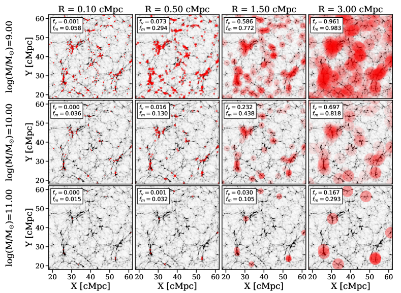
Figure 1: 2D slices of the Nyx density field at $z=4.5$ for different spatial distributions of metals. Each slice is 1.0 cMpc thick and shows only a portion (40 cMpc $\times$ 40 cMpc) of the entire 2D projection, and is the same for every panel. Each row corresponds to a different minimum halo mass that contributes to enrichment (log$\,M$) and each column corresponds to a different maximum radius out to which enrichment occurs ($R$). For each model, the enriched regions are shown as red shaded regions. For a fixed row, the same set of halos contribute to the underlying enrichment, but out to increasing distances from left to right. For a fixed column, the enrichment radius is fixed but different halos masses give rise to the enrichment. The corresponding volume-filling fraction ($f_{V}$) and mass-filling fraction ($f_{m}$) of metals are indicated. The filling fractions increase with decreasing log$\,M$ and increasing $R$.

We compute the corresponding mass- and volume-filling fractions of metals from our enrichment topologies. The mass-filling fraction ($f_{m}$) is calculated as the total densities of the enriched pixels (denoted with superscript $Z$) over the total density of all pixels. The volume-filling fraction ($f_{V}$) is calculated as the total number of enriched pixels over all pixels.

$$f_{m}=\frac{\Sigma_{i}\rho_{i}^{Z}}{\Sigma_{i}\rho_{i}}=\frac{\Sigma_{i}\Delta_{i}^{Z}}{\Sigma_{i}\Delta_{i}}$$ (1)

$$f_{V}=\frac{N^{Z}}{N_{\rm{pix}}},$$ (2)

where $\Delta_{i}\equiv\rho_{i}/\langle\rho\rangle_{\mathrm{V}}$. As expected, Figure 1 shows both filling fractions increasing with increasing $R$ but decreasing as log${}_{10}\,M_{\mathrm{min}}$ increases, as fewer halos contribute to the enrichment. As $f_{m}$ is weighted towards overdense regions, it is always larger than $f_{V}$ for the same topology. Additionally, for topologies with similar $f_{V}$, the metals appear more concentrated as opposed to more uniformly-distributed in those with larger $f_{m}$, as overdense regions are also more clustered. Figure 3 shows the trends of the filling fractions with log${}_{10}\,M_{\mathrm{min}}$ and $R$.

Given an inhomogeneous enrichment with input metallicity [C/H], one can also compute the effective metallicity of the IGM

$$Z_{\mathrm{eff}} \equiv\frac{N_{\mathrm{C}}}{N_{\mathrm{H}}}$$

$$=\frac{Z_{\odot}10^{\rm{[C/H]}}\langle n_{\mathrm{H}}\rangle\Sigma_{i}(\Delta_{i}^{Z}\cdot V_{\mathrm{cell},i})}{\langle n_{\mathrm{H}}\rangle\Sigma_{i}(\Delta_{i}\cdot V_{\mathrm{cell},i})}$$

$$=Z_{\odot}\cdot 10^{\rm{[C/H]}}\cdot\frac{\Sigma_{i}\Delta_{i}^{Z}}{\Sigma_{i}\Delta_{i}}$$

$$=Z_{\odot}\cdot 10^{\rm{[C/H]}}\cdot f_{m}$$

$$\mathrm{[C/H]}_{\rm{eff}}\equiv\mathrm{log}_{10}\left(\frac{Z_{\rm{eff}}}{Z_{\odot}}\right)=\mathrm{log}_{10}\left(10^{\mathrm{[C/H]}}\cdot f_{m}\right),$$ (3)

where $N_{\mathrm{C}}$ is the total number of carbon atoms, $\Delta_{i}^{Z}$ is the overdensity of enriched pixel $i$, and $V_{\mathrm{cell},i}$ is the volume of a cell in the simulation. Figure 3 shows [C/H]_eff for an input [C/H] = $-3.50$ while varying the morphological parameters.

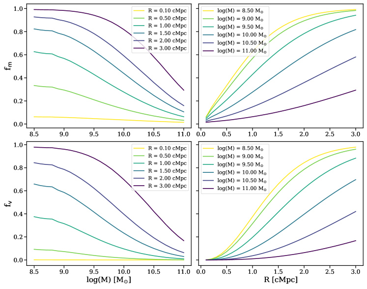
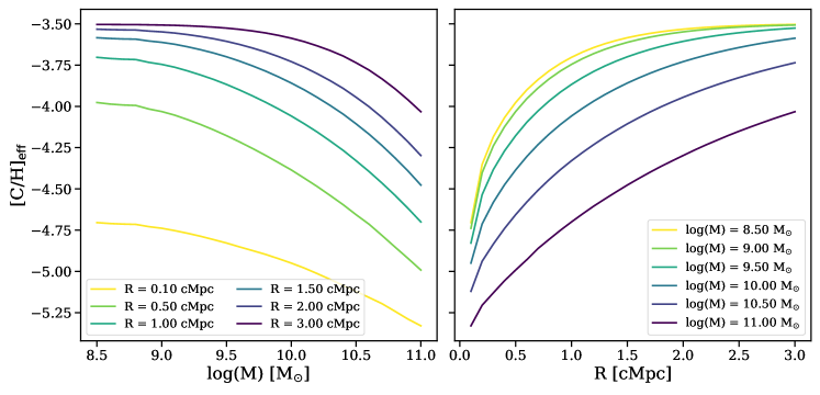
Figure 2: Trends of the mass-filling fraction ($f_{m}$; top panel) and volume-filling fraction ($f_{V}$; bottom panel) as a function of the enrichment topology model parameters. The left panel shows the relation as a function of log$\,M$ at fixed $R$ (different colored lines). For very small $R$, the filling fractions remain almost constant with log$\,M$, otherwise they decrease with increasing log$\,M$ (less contributing halos). The right panel shows the relation as a function of $R$ at fixed log$\,M$ (different colored lines). The filling fractions decrease with decreasing $R$ (smaller enrichment region). For the same enrichment topology, $f_{m}>f_{V}$ because $f_{m}$ is weighted towards overdense region whereas $f_{V}$ is a simple number count.

Figure 3: The effective metallicity as a function of the enrichment topology model parameters, log$\,M$ (left) and $R$ (right). The maximum value on the y-axis indicates the input metallicity of [C/H] = $-3.50$. The effective metallicity reflects the underlying trend of the mass-filling fraction $f_{m}$, with the input metallicity affecting the overall normalization (see Eqn 3).

2.3 Creating C IV skewers

The methodology to simulate the C iv forest is similar to the methods detailed in §2.4 of H2020 to simulate the Mg ii forest. We first randomly draw Nyx skewers along one face of our simulation box, for a total of 10,000 skewers. These provide us with the baryon density, temperature, and line-of-sight peculiar velocity. We additionally need the fraction of carbon in the triply-ionized state for each cell of the skewer. We compute the ionization fractions of carbon at $z=4.5$ using CLOUDY (C17 version; Ferland et al., 2017) on a grid of hydrogen densities (log $n_{\mathrm{H}}$ = $-7$ cm^-3 to log $n_{\mathrm{H}}$ = 0 cm^-3 in increments of 0.1 dex), gas temperatures ($10^{2}$ K to $10^{7}$ K in increments of 0.1 dex), and metal abundance ([C/H] from $-3.5$ to $-1.5$). The gas is irradiated by a uniform UV background from galaxies and quasars using the prescription of Haardt & Madau (2012). As the C iv fraction does not vary significantly with metal abundance (for an optically thin IGM in photoionization equilibrium), we use the results obtained with [C/H] = $-3.5$ for the rest of this paper.

Figure 4 shows the dominant carbon ions in the density and temperature phase space of our CLOUDY grid, overplotted against the distribution of our randomly-selected skewers. The dominant ion is defined as the ion that has the largest fraction among all available ions at each grid point (the value of this maximum fraction varies). The C iv ion is the most dominant ion in the very low-density (log $n_{\mathrm{H}}\sim-6$ to $-5$ cm^-3) and cool (10${}^{2}-10^{4.5}$ K) gas, with an ionic fraction of $x_{\mathrm{\text{C\,{iv}}}}\sim 0.45$ at mean density. The C ii and C iii ions dominate in the condensed (log $n_{\mathrm{H}}>-2.50$ cm^-3) and moderately low-density (log $n_{\mathrm{H}}\sim-4$ to $-2.50$ cm^-3) gas phases, respectively, whereas high-ionization ions typically reside in hot $T\gtrsim 10^{5}$ K gas in both the diffuse and condensed phases. The horizontal bands of C v and C vi ions at $T\sim 10^{5}$ K that span log $n_{\mathrm{H}}>10^{-5}$ cm^-3 are due to collisional ionization. We linearly interpolate the CLOUDY output of $x_{\mathrm{\text{C\,{iv}}}}$ as a function of density and temperature onto the Nyx skewers. Given these ingredients, the optical depth for each component of the C iv doublet can be computed as

$$\tau_{v}=\tau_{\rm C,0}\int E_{0,1}\frac{x_{\mathrm{\text{C\,{iv}}}}\Delta}{\sqrt{\pi}}\mathrm{exp}\left[-\left(\frac{v^{\prime}-v}{b}\right)^{2}\right]\frac{dv^{\prime}}{b},$$ (4)

where $E_{0,1}$ is the enrichment topology (in practice, a True/False bit that determines if a location is enriched or not), $b$ is the Doppler parameter and $\tau_{\rm C,0}$ is the C iv analog of the Gunn-Peterson optical depth

$$\tau_{\rm C,0} =\frac{\pi e^{2}f_{lu}\lambda_{lu}n_{\rm C}}{m_{e}cH(z)}.$$ (5)

The $f_{lu}$ term is the oscillator strength, $\lambda_{lu}$ is the wavelength of the transition, and $n_{\rm C}$ is the number density of carbon, which is related to the metallicity as $n_{\rm C}=(Z/Z_{\odot})(n_{\rm C}/n_{\rm H})_{\odot}\langle n_{\rm H}\rangle$. At $z=4.5$ and assuming an input [C/H] = $-3.5$ in enriched regions,

$$\tau_{\rm C,0} =0.013\left(\frac{Z/Z_{\odot}}{10^{-3.5}}\right)\left(\frac{(n_{\rm C}/n_{\rm H})_{\odot}}{2.7\times 10^{-4}}\right)\left(\frac{f_{lu}}{0.1899}\right)$$

$$\qquad\qquad\;\left(\frac{\lambda_{lu}}{\mathrm{1548\r{A}}}\right)\left(\frac{1+z}{1+4.5}\right)^{3/2}.$$ (6)

Note that metallicity is a multiplicative factor in front of the optical depth, so we can use the same set of skewers to generate the C iv forest at different metallicities by simply rescaling the optical depth. In practice, rather than computing the optical depth for both transitions in the C iv doublet, we only compute the optical depth of the stronger (bluer) line, $\tau_{1548}$, and rescale it by the oscillator strength ratio of the two lines $f_{1550}/f_{1548}$ = 0.499 to obtain $\tau_{1550}$, which is then shifted redward equivalent to the doublet separation $dv=498$ km/s. The total optical depth of the C iv forest is $\tau_{\mathrm{\text{C\,{iv}}}}=\tau_{1548}+\tau_{1550}$. We adopt the same approach as H2020 in discretizing the integral in Equation 4 to handle the possibility that our simulation native velocity grid ($dv_{\rm pix}$ = 3.16 km/s) barely resolves the small Doppler parameter of the C iv ion ($b$ = 3.71 km/s at 10,000 K). The optical depth of the discretized grid cell is computed as (cf. Appendix B of Lukić et al., 2015)

$$\tau_{v}=\tau_{X,0}\sum_{i}\frac{x_{\mathrm{\text{C\,{iv}}},i}\Delta_{i}}{2}\left[\mathrm{erf}(y_{i-1/2})-\mathrm{erf}(y_{i+1/2})\right].$$ (7)

Figure 5 shows skewers of the relevant quantities for a random sightline through our box, assuming an enrichment model with log${}_{10}\,M$ = 9.50 $M_{\odot}$, $R$ = 0.80 Mpc, and [C/H] = $-3.50$. The enrichment topology skewer is essentially a Boolean skewer that determines which pixels are enriched, which subsequently determines the structures in the other skewers. We compute the C iv column density for the $i$-th pixel as $N_{\mathrm{\text{C\,{iv}}},i}=(n_{\mathrm{\text{C\,{iv}}},i}\,E_{(0,1),i})\times$pixel scale, where $n_{\mathrm{\text{C\,{iv}}},i}=\Delta_{i}\langle n_{\rm H}\,\rangle(Z_{\odot}\,10^{[\mathrm{C/H}]})\,x_{\mathrm{\text{C\,{iv}}},i}$ and our pixel scale = 6.48 kpc (such that a typical absorber will span multiple pixels). We show a perfect noiseless spectrum at the native grid resolution and a noisy spectrum with SNR/pix = 50 that has been degraded to the spectral resolution of Keck/HIRES or VLT/UVES, which is FWHM = 10 km/s ($R$ = 30,000). We assume the same observational setups for our mock data in §3.3.

For the IGM model shown in Figure 5, one can see remarkable fluctuations of order a few percent from the perfect spectrum. However, these get challenging to detect in real data, even with moderately high SNR/pix of 50 and exquisite spectral resolution. In this regime, a statistical method like the correlation function is better suited for the task. Additionally, that the column density of the diffuse IGM is $\sim 10^{10}-10^{11}$ cm^-2 makes it extremely challenging to detect with the standard line-fitting method, even with state-of-the-art instrumentation on the largest ground-based telescopes. The two deepest spectra of quasars ever taken are that of B1422+231 ($z$ = 3.62; Ellison et al., 2000) and HE0940-1050 ($z$ = 3.09; D’Odorico et al., 2016). The former has a SNR of $200-300$ redward of Ly$\alpha$ with a detection limit at log($N_{\mathrm{\text{C\,{iv}}}}$/cm^-2) $\approx$ 11.6. The spectrum of HE0940-1050 has a SNR of $320-500$ in the C iv forest region, where they are sensitive down to log($N_{\mathrm{\text{C\,{iv}}}}$/cm^-2) $\approx$ 11.4. Although these high SNR observations likely probe the entire spectrum of absorbers, from the strongest CGM absorbers to the diffuse IGM absorbers at the low column density end, they are at a much lower redshift than $z=4.5$ that we simulate here. As such, nearly all detections of absorbers with $N_{\rm\text{C\,{iv}}}\gtrsim 13-14$ cm^-2 at $z\gtrsim 3$ are most likely from the CGM.

Figure 4: The dominant carbon ions (indicated by colorbar) as a function of temperature and hydrogen density, overplotted against the distribution of our 10,000 random Nyx skewers, with the gray scale showing the density of points. The dominant ion is determined based on the ionization fraction output by CLOUDY at $z=4.5$. The temperature and density phase space is demarcated into “diffuse” IGM, “condensed” gas, and “WHIM” (warm hot intergalactic medium) gas by dashed lines. The C iv ion (purple region) dominates in the very low-density and cold IGM, and the yellow lines show the contours for C iv fraction of 0.30 and 0.50. At high temperatures $>10^{5}$ K, collisional ionization takes over and is denoted by the horizontal band.

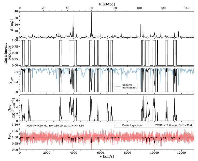
Figure 5: Skewers of various quantities for a random sightline. The overdensity skewer is obtained directly from the Nyx box. The enrichment topology skewer is a Boolean skewer that determines which pixels are enriched (1 for enriched and 0 for not enriched), and here we show the topology for an IGM model with log$\,M$ = 9.50 $M_{\odot}$, $R$ = 0.80 Mpc, and [C/H] = $-3.50$. The corresponding C iv fraction $X_{\mathrm{\text{C\,{iv}}}}$ for this IGM model is shown in the middle panel, overplotted against the uniform enrichment case. We also show the column density skewer, computed as $N_{\mathrm{\text{C\,{iv}}},i}=(n_{\mathrm{\text{C\,{iv}}},i}\,E_{(0,1),i})\,\times$ pixel scale, where $E_{0,1}$ is the enrichment topology. The C iv forest is shown in the last panel, with black being the noiseless spectrum at the native grid resolution and red being the noisy spectrum convolved with a FWHM of 10 km/s, i.e. that of Keck/HIRES or VLT/UVES. Even with a moderately high SNR of 50 and exquisite spectral resolution, it is challenging to detect the C iv forest signal.

3 Results

3.1 Correlation function of the C IV forest

To compute the correlation function of the C iv forest, we first define the flux fluctuation,

$$\delta_{f}\equiv\frac{F-\langle F\rangle}{\langle F\rangle},$$ (8)

where $\langle F\rangle$ is the volume-averaged mean flux. The correlation function is then

$$\xi(dv)=\big{\langle}\delta_{f}(v)\delta_{f}(v+dv)\big{\rangle},$$ (9)

where the average is over all available pixel pairs separated by $dv$.

Figure 6 shows the correlation functions of the C iv forest for varying model parameters, assuming noiseless skewers from our mock dataset (see §3.3) that are convolved with a Gaussian line spread function of FHWM=10 km/s. We see the correlation functions peaking at $dv=498$ km/s, corresponding to the doublet separation that sets the characteristic scale of the C iv forest.

Metallicity is a normalizing factor in front of the optical depth (Equation 6) such that optical depth increases with metallicity and gives rise to a stronger signal. In the limit of small optical depths as is for the C iv forest, $F\approx 1-\tau\propto Z$, so metallicity affects the correlation function by rescaling the peak amplitude approximately as the square of the metallicity, e.g. the peak amplitude for [C/H] = $-3.20$ is $\sim(10^{-3.20}/10^{-3.50})^{2}\sim 4$ times larger than for [C/H] = $-3.50$. Varying log${}_{10}M_{\mathrm{min}}$ alone also affects the peak amplitude, with a weaker peak as log${}_{10}M_{\mathrm{min}}$ increases. On the other hand, $R$ affects both the shape and amplitude; increasing $R$ results in an increase in power on both sides of the peak in the correlation function at the doublet separation. In general, the correlation function increases with increasing filling factors. This is essentially a metallicity effect, as increasing the filling factors results in more enrichment and higher metallicities, with $R$ additionally affecting the small- and large-scale powers. It is apparent that the effects of metallicity and enrichment topology are degenerate with each other, but we show that they can still be individually constrained to good precision in §3.3.

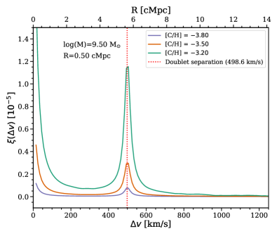
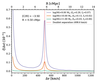
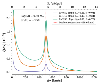
Figure 6: Correlation function of the C iv forest at varying metallicity (top) and enrichment topology (middle for varying log${}_{10}M_{\mathrm{min}}$ and bottom for varying $R$), computed assuming noiseless spectra convolved with FWHM = 10 km/s. The peak in the correlation corresponds to the C iv doublet separation, as indicated by the vertical dotted lines. The peak becomes more prominent as metallicity increases, scaling roughly as the metallicity squared. Increasing log${}_{10}M_{\mathrm{min}}$ leads to a decrease in the peak amplitude, while increasing $R$ increases the power on both sides of the peak in the correlation function at the doublet separation.

Figure 7 shows the effect of spectral resolution on the correlation function of the C iv forest, using three resolutions that resemble Keck/HIRES and VLT/UVES (FWHM = 10 km/s), VLT/X-SHOOTER (Vernet et al., 2011) (FWHM = 30 km/s), and Keck/DEIMOS (DEep Imaging Multi-Object Spectrograph; Faber et al., 2003) (FWHM = 60 km/s). As spectral resolution decreases, the peak of the correlation function becomes broadened and the small-scale power reduced. The peak is still visible even with FWHM = 60 km/s, although one would require high SNR data to reliably detect it.

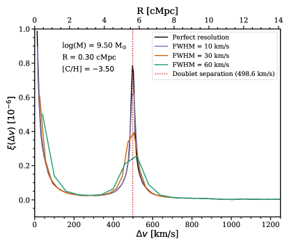
Figure 7: Correlation function of the C iv forest at varying spectral resolutions compared to that of a perfect spectrum (i.e. at the native resolution of our simulation), assuming noiseless spectrum. Resolutions of 10 km/s, 30 km/s, and 60 km/s are representative of Keck/HIRES (or VLT/UVES), VLT/X-SHOOTER, and Keck/DEIMOS, respectively. The particular IGM model used to compute the correlation functions is indicated.

3.2 Contamination from CGM C IV absorbers

So far our results in the previous section do not include the effect of C iv absorbers from the circumgalactic medium (CGM) of galaxies, as our skewers consist only of pure IGM absorbers. As we are interested in the background metallicity of the IGM, absorbers near galaxies can bias our results as they tend to be more enriched and give rise to higher column densities (e.g. Lehner et al., 2016; Wotta et al., 2016; Prochaska et al., 2017). We investigate their effects here by injecting them into our skewers.

3.2.1 Equivalent width frequency distribution

We first model their abundance, given by their equivalent width frequency distribution, as a Schechter function with the following form (Kacprzak & Churchill, 2011; Hasan et al., 2020):

$$\frac{d^{2}n}{dW_{\lambda}dz}=\frac{n^{*}}{W*}\left(\frac{W_{\lambda}}{W^{*}}\right)^{\alpha}\mathrm{exp}\left(-\frac{W_{\lambda}}{W^{*}}\right),$$ (10)

where $n$ is the number of absorbers and $W_{\lambda}$ is the rest-frame equivalent width.

To guide selection of the suitable model parameters, we look to existing observations. Various studies have measured the frequency distribution of C iv absorbers at $z\sim 4.5$, which requires echelle spectra covering the z-band. We are mostly interested in weak absorbers, as they are expected to be the dominant contaminating signal and because strong absorbers can be easily identified and masked. To detect weak absorbers, the observations typically need to be taken with high-resolution and/or high SNR. The two deepest quasar spectra to date are that of B1422+231 ($z$ = 3.62; Ellison et al., 2000), with a detection limit of log($N_{\mathrm{\text{C\,{iv}}}}$/cm^-2) $\approx$ 11.6, and HE0940-1050 ($z$ = 3.09; D’Odorico et al., 2016), where they are sensitive down to log($N_{\mathrm{\text{C\,{iv}}}}$/cm^-2) $\approx$ 11.4. Despite being very high SNR observations with the possibility of probing actual diffuse IGM absorbers, they are at a lower redshift than $z=4.5$ that we simulate here.

Higher redshift observations exist, but at lower SNR. D’Odorico et al. (2013) observed six quasars at $4.35<z<6.2$ with VLT/X-shooter and computed the column density distribution function (CDDF; $d^{2}n/dN/dX$) in two redshift bins over the range $12.6<\mathrm{log}(N_{\mathrm{\text{C\,{iv}}}}/\rm{cm}^{-2})<15$. At $z<5.3$, they are 85% complete down to log($N_{\mathrm{\text{C\,{iv}}}}$/cm^-2) = 13.3. Simcoe (2011) measured the CDDF at $z=4.25$ with three quasar spectra obtained with the Magellan MIKE spectrograph. Their detection limit is roughly log($N_{\mathrm{\text{C\,{iv}}}}$/cm^-2) = 12, while being substantially complete between log($N_{\mathrm{\text{C\,{iv}}}}$/cm^-2) = 13 and 14. At the high column density end, Cooksey et al. (2013) measured the equivalent width distribution of log($N_{\mathrm{\text{C\,{iv}}}}$/cm^-2) $>$ 14 (corresponding to $W_{\lambda}>$ 0.6 $\mathrm{\AA}$) absorbers at $2.97\leq z\leq 4.54$ with SDSS DR7. Their 50% completeness limit is log($N_{\mathrm{\text{C\,{iv}}}}$/cm^-2) = 14. One of the most comprehensive abundance measurements of C iv absorbers is from Hasan et al. (2020), who measured the equivalent width distribution of C iv absorbers from 1.1 $\leq z\leq$ 4.75 using 369 QSO spectra from Keck/HIRES and VLT/UVES. Their measurements in the highest redshift bin, 2.5 $\leq z\leq$ 4.75, are 50% complete for weak absorbers with $W_{\lambda}$ = 0.06 $\mathrm{\AA}$ (or $N_{\mathrm{\text{C\,{iv}}}}=1.5\times 10^{13}$ cm^-2, see Eqn 13).

We convert literature measurements, usually expressed in units of $d^{2}n/dN/dX$, to be consistent with the units of our model function (Eqn 10), via the following conversion

$$\frac{d^{2}n}{dW_{\lambda}dz}=\frac{d^{2}n}{dNdX}\left(\frac{dW}{dN}\right)^{-1}\frac{dX}{dz}.$$ (11)

The redshift absorption pathlength $dX$ is defined as $X(z^{\prime})=\int^{z}_{0}(1+z)^{2}[H_{0}/H(z)]dz$ (Bahcall & Peebles, 1969). Assuming $\Lambda$CDM, $dX/dz=(1+z)^{2}[\Omega_{\mathrm{m}}(1+z)^{3}+\Omega_{\Lambda}]^{-1/2}$. We obtain $dW/dN$ numerically. While $W$ scales linearly with $N$ on the linear part of the curve-of-growth, this dependence changes once absorbers are saturated (i.e. reach a high enough column density) and so one needs to assume the $b$-values in order to determine $W(N)$ and $dW/dN$. Following H2020, we model the $b$-value as a sigmoid function,

$$b=b_{\mathrm{weak}}+(b_{\mathrm{strong}}-b_{\mathrm{weak}})\times\\ \left[1+\mathrm{exp}\left(-\frac{\mathrm{log\,}N_{\mathrm{\text{C\,{iv}}}}-\mathrm{log\,}N_{\mathrm{strong}}}{\Delta\mathrm{log\,}N}\right)\right]^{-1}.$$ (12)

The $\Delta\mathrm{log\,}N$ variable is the interval over which log($N_{\mathrm{\text{C\,{iv}}}}$) transitions from log$\,N_{\mathrm{weak}}$ to log$\,N_{\mathrm{strong}}$. For our model, we use $b_{\mathrm{weak}}=10$ km/s, $b_{\mathrm{strong}}=150$ km/s, log$N_{\mathrm{strong}}$ = 14.5, and $\Delta\mathrm{log\,}N$ = 0.35. Our values are motivated by the fact that the C iv line becomes saturated at $W_{1548}$ = 0.6 $\mathrm{\AA}$ (Cooksey et al., 2013), which translates to $N_{\mathrm{\text{C\,{iv}}}}$ = 1.5 $\times$ 10¹⁴ cm^-2 assuming one is on the linear part of the curve-of-growth where

$$W_{\lambda}=0.04\,\mathrm{\AA}\left(\frac{N_{\mathrm{\text{C\,{iv}}}}}{10^{13}\,\rm{cm}^{-2}}\right).$$ (13)

The maximum optical depth at the line center of a Voigt profile is

$$\tau_{0}=1.47\left(\frac{N_{\mathrm{\text{C\,{iv}}}}}{10^{14}\,\rm{cm}^{-2}}\right)\left(\frac{30\,\mathrm{km/s}}{b}\right).$$ (14)

Absorption lines thus saturate around $N_{\mathrm{\text{C\,{iv}}}}$ = 1.5 $\times$ 10¹⁴ cm^-2 ($W_{\lambda}=0.6$ $\mathrm{\AA}$) for $b$ = 30 km/s.

Our final CGM model is shown in Figure 8. We fine-tune the weak-end of the model to match with data from Simcoe (2011) and D’Odorico et al. (2013) and the strong-end of the model to match with the best-fit from Cooksey et al. (2013), resulting in ($\alpha$, $W^{*}$, $n^{*}$) = ($-1.10$, 0.45, 5). Our Schechter-function fit is slightly steeper than that of Hasan et al. (2020), otherwise the parameters are generally similar. We randomly draw absorbers from our CGM model ranging from $W_{\lambda,\mathrm{min}}=0.001$ $\mathrm{\AA}$ to $W_{\lambda,\mathrm{max}}=5.0$ $\mathrm{\AA}$ and artificially inject them into our mock skewers. We ignore absorber clustering and place absorbers at random velocity locations along our skewers.

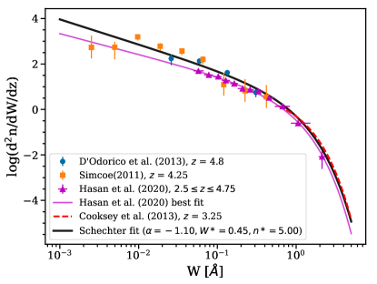
Figure 8: Number of C iv absorbers per unit equivalent width per unit redshift (equivalent width frequency distribution) as a function of rest-frame equivalent width. Plotted as various points are existing (high SNR and high resolution) observations at comparable redshifts as ours. We show our best-fit CGM model as the solid black line, which is consistent with existing observations and best-fits to observations (purple and red lines).

Following the procedures in Appendix A of H2020, the CGM absorbers of our model give [C iv/H] = $-5.71$ (with solar values from Asplund et al., 2009), which corresponds to a cosmological mass fraction of $\Omega_{\text{C\,{iv}}}=3.97\times 10^{-8}$. Assuming a C iv to C fraction of 0.5 (which is reasonable given Figure 4), we obtain [C/H] = $-5.41$ and $\Omega_{\rm C}=7.94\times 10^{-8}$. As a comparison, Simcoe (2011) obtained $\Omega_{\mathrm{C}}=2.7\times 10^{-8}$ at $z=4.3$ while Schaye et al. (2003) obtained $\Omega_{\mathrm{C}}=2.21\times 10^{-7}$ for gas with log($\Delta$) = $0.5-2.0$ (see Figure 4) at $z=3$. Potential reasons that could lead to our $\Omega_{\rm C}$ being $\sim 3\times$ higher than that obtained by Simcoe (2011) are our CGM model including very strong absorbers up to $W_{\lambda}=5\,\mathrm{\AA}$ as well as having a steeper slope at the lowest column density end.

3.2.2 Flux probability distribution function

We define the flux (decrement) probability distribution function (PDF) in log₁₀-unit, where $\mathrm{frac}(a,b)=\int_{a}^{b}\frac{dP}{d\,\mathrm{log}_{10}(1-F)}d\,\mathrm{log}_{10}(1-F)$ and frac($a,b$) is the fraction of pixels between $a$ and $b$. Figure 9 shows the flux PDF of the IGM, the CGM, and Gaussian random noise with $\sigma=$ (SNR)^-1 and SNR = 50 per pixel. The top axis of the PDF plot is $W_{\lambda,\mathrm{pix}}\equiv(1-F)\,d\lambda$, where $d\lambda$ is the width of a spectral pixel; for our mock dataset with FWHM=10 km/s, $d\lambda=0.017\mathrm{\AA}$ at C iv 1548 $\mathrm{\AA}$. The PDFs for a uniformly-enriched IGM and for an inhomogeneously-enriched IGM with the same model as Figure 5 are shown, where the effective metallicity of the non-uniform IGM matches the metallicity of the uniform IGM. The PDF for the CGM component is further broken down into different $W_{\lambda}$ ranges to show the impact of absorbers with different strengths. Since the flux PDF is plotted on a log scale, negative fluctuations of the noise PDF are not shown, but they are simply symmetrical to the positive fluctuations about zero.

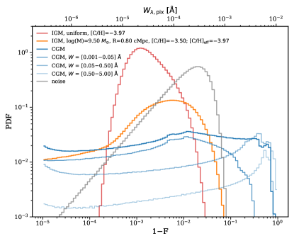
Figure 9: Probability distribution function of the flux decrement for a uniformly-enriched IGM (red), a non-uniformly enriched IGM for one particular model (orange), the CGM (blue), and random noise with SNR/pix = 50 (gray). The uniform IGM model has the same metallicity as the effective metallicity of the non-uniform IGM. The CGM PDF is broken down into different equivalent width ranges, shown by the different shades of blue lines. The IGM PDFs have a distinct shape compared to the CGM PDF. They peak about small $1-F$ values, dominating over the CGM by at least a few times, and then cut off at large $1-F$ values, while the CGM PDF remains mostly flat across the entire range.

Compared to the IGM flux PDFs that peak at small $1-F$ values and drop off at large $1-F$, the PDF for the CGM absorbers remains mostly flat up to large $1-F$ values. Weak absorbers dominate the PDF in the region of overlap with the IGM absorbers, followed by moderate and strong absorbers. As such, they are the main contaminant of our correlation function analysis. Since weak absorbers cannot produce large flux decrements, their PDF drops off at large $1-F$ values, in contrast to strong absorbers whose PDF rises and peaks at very large $1-F$ values of $\sim 1$.

In contrast to the uniformy-enriched IGM, the PDF of the inhomogeneously-enriched IGM has a more rounded peak and a tail towards very small $1-F$ values. The rounded peak is possibly an effect of pixels being enriched pre-dominantly around halos, while the very small flux decrements arise from mixing of metal-enriched with metal-free regions. As absorption occurs in redshift space, the optical depth of a given pixel can arise from multiple gas elements due to redshift-space distortion coming from the gas peculiar velocities. The mixing between metal-free pixels and metal-enriched pixels therefore results in this tail of very transmissive values. The flux PDF for the uniformly-enriched IGM cuts off at a value that corresponds to the most transmissive pixel (at small $F$, the flux decrement $1-F\approx\tau$) and does not have a tail because there is no completely metal-free region. Its PDF dominates over that of the CGM by more than an order of magnitude and that of noise by a factor of a few.

Figure 10 shows the changes in the flux decrement PDF of the inhomogeneously-enriched IGM with model parameters. From left to right, we vary log$\,M$, $R$, and [C/H] while holding the other two parameters fixed. Increasing log$\,M$ amounts to renormalizing the entire PDF downward — because massive halos are rare, fewer pixels are enriched when restricting to higher mass halos. If only the most massive halos (log$\,M\geq$ 10.5 $M_{\odot}$; yellow line) contribute to enrichment, the CGM absorbers will start to be more abundant than their IGM counterparts. Increasing the enrichment radius $R$ has a similar effect as decreasing log$\,M$, resulting in a larger number of enriched pixels (the metal filling fractions approach unity as $R$ increases, see Figure 3). This can be seen as the entire PDF being shifted upward. It also asymptotes to the flux PDF of a uniformly-enriched IGM for very large $R$ where the metal filling fractions approaching unity, see Figure 3), with the peak of the PDF becoming more pronounced (less biased enrichment) and the tail of the distribution dropping rapidly for very small $1-F$ values (smaller number of very transmissive pixels). Changing [C/H] simply shifts the PDF left or right, which can be understood because optical depth, hence flux in the low optical depth limit, scales linearly with metallicity. A higher metallicity produces a higher optical depth that then shifts the entire PDF to the right, and vice versa. The importance of noise depends on the IGM model. Generally, the flux fluctuations of models with smaller log$\,M$ and larger $R$ (i.e. larger [C/H_eff) dominate over noise fluctuations at the peak of the IGM PDF. Nevertheless, the IGM peak may be shifted closer to or farther from that of noise depending on the input metallicity.

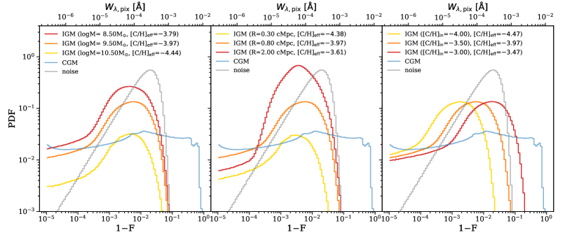
Figure 10: Effects on the IGM flux decrement PDF at varying values of log$\,M$ (left), $R$ (middle), and input metallicty [C/H]_in (right). When log$\,M$ ($R$) is varied, we fix $R$ = 0.80 cMpc (log$\,M$ = 9.50 $M_{\odot}$) and [C/H]${}_{\mathrm{in}}=-3.50$. When [C/H]_in is varied, we fix log$\,M$ = 9.50 $M_{\odot}$ and $R$ = 0.80 cMpc. The CGM and noise PDFs are the same in all panels. Increasing log$\,M$ shifts the PDF downward, while increasing $R$ has the opposite effect. Increasing [C/H]_in results in more absorbent pixels and shifts the PDF rightward.

3.2.3 Masking CGM absorbers

The flux PDF provides a way to separate the CGM from the IGM absorbers because the flux PDF of the two populations have different shapes. The simplest cut involves a flux cut that filters out large $1-F$ values arising from the CGM, as shown by the left panel in Figure 11. Here we have added noise with SNR/pix = 50 to our skewers.

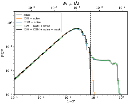
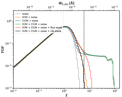
Figure 11: Filtering schemes to remove CGM absorbers based on the flux decrement (left) and significance (right) PDFs. A random noise of SNR/pix = 50 has been added to all PDFs in both panels. The black PDFs show the resultant PDFs for the combined IGM + CGM + noise PDF after applying the cuts indicated by the vertical dashed lines, i.e. we remove all pixels with $1-F>0.07$ in the left panel and all pixels with $\chi>6$ in the right panel. These cuts remove large fluctuations caused by CGM absorbers, which are manifested in the tail of the IGM + CGM + noise PDF (green), in contrast to the IGM + noise PDF (orange) that drops off. Although the flux cut (red; right panel) removes a vast majority of the large fluctuations in the $\chi$ field, significant contamination remains when compared with the IGM + noise PDF (orange). The gray shaded regions on the IGM + CGM + noise PDF (green) are 1$\sigma$ errors of our mock dataset described in §3.3. The IGM model here is the same as the inhomogenous IGM model in Figure 9.

Although the noisy IGM PDF is indistinguishable from the noisy CGM PDF at small $1-F$ values, values with $1-F>0.07$ in the combined noisy PDF mostly lie outside the IGM PDF and are due to CGM absorbers. As such, we can simply mask out pixels with $1-F>0.07$, which only minimally reduces the number of IGM pixels in our mock spectra by 3%. Figure 12 shows the correlation function after masking out pixels with the flux cut. Note that the correlation function of the unmasked IGM+CGM (gray solid line) has been rescaled. The correlation function of the flux-masked pixels (pink dashed line) is biased slightly high compared to that of the pure IGM (orange solid line). Rather than arising from weak absorbers, which overlap with the IGM absorbers but are less abundant, this bias is instead due to unmasked pixels from the wings of the strong CGM absorbers. The flux cut manages to filter out the absorption cores of these absorbers but misses their shallow wings. To reduce this bias we can supplement the flux cut with another filtering method.

The second filtering scheme involves explicitly identifying CGM absorbers. In standard practice, this is done by convolving mock spectra with a matched filter $W(v)$ that corresponds to the transmission profile of a doublet (Zhu & Ménard, 2013), such that extrema in the significance field (H2020),

$$\chi(v)=\frac{\int[1-F(v^{\prime})]W(|v-v^{\prime}|)dv^{\prime}}{\sqrt{\sigma_{F}^{2}(v^{\prime})W^{2}(|v-v^{\prime}|)dv^{\prime}}},$$ (15)

are assumed to be from an absorber. In the above definition, $\sigma_{F}^{2}$ is the flux variance due to noise. The matched filter $W(v)$ is $1-e^{-\tau(v)}$, where $\tau(v)$ is the optical depth of a C iv doublet with a Gaussian velocity distribution, assuming $N_{\mathrm{\text{C\,{iv}}}}=10^{13.5}$ cm^-2 and Doppler parameter $b=\sqrt{2}\sigma=6.02$ km/s assuming $\sigma=\mathrm{FWHM}/2.35$ and FWHM = 10 km/s for the resolution of our mock spectra in §3.3. The right panel of Figure 11 shows the $\chi$-PDF of our mock spectra. Similar to the flux PDF, CGM absorbers give rise to large $\chi$ values. We can therefore remove them by (i) implementing a $\chi$ cut with $\chi>6$ and (ii) removing pixels $\pm 200$ km/s around each extrema — this is what we refer to as a “chi cut”. Our final mask is a “flux + chi” mask, where “flux + chi” $\equiv$ flux cut OR chi cut. As shown in Figure 12, the correlation functions using the various masks (blue solid line) very closely match that of the pure IGM (orange solid line) within the measurement errors of our mock dataset in §3.3. A flux, chi, and flux + chi mask removes 3%, 35%, and 35% of the pixels in our spectra, respectively.

Although masking reduces the overall pathlength and increases the statistical error, it does not bias correlation function measurements. Indeed, compared to the power spectrum, which in the simplest implementation would be sensitive to masking, the correlation function does not care about gaps in the spectra created from masking.

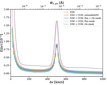
Figure 12: Comparison of the C iv forest correlation function before and after masking. Note that the unmasked IGM + CGM (gray) has been rescaled down by a factor of 50 to aid visualization. The effectiveness of the masking procedures is judged against the true signal from the pure IGM (orange), where we use the model with (log$\,M_{\rm{min}}$, $R$, [C/H]) = (9.50 $M_{\odot}$, 0.80 Mpc, $-3.50$). The cuts used in the masking are the same as in Figure 11. Despite removing majority of the CGM signal, flux masking alone (pink dashed) results in residual bias in the masked spectra. Using either a chi cut only (green dashed) or combining the flux cut with a chi cut (blue) suppresses this bias and recovers the underlying IGM correlation function within the 1$\sigma$ errors of our mock dataset.

For the particular IGM model we have chosen, the flux cutoff at $1-F>0.07$ and the $\chi$ cutoff at $\chi>6$ work well in removing the CGM absorbers and reproducing the pure-IGM correlation function. In real data, the choice of where to place the cutoffs can be made by computing the corresponding flux and $\chi$-PDFs and inspecting the region where the PDF starts to drop and then flatten. The choices of the cutoff values can also be forward-modeled in mock spectra and accounted for. As we have shown that CGM absorbers can be filtered out for our mock dataset with SNR/pix of 50, we did not include them in the next section where we perform statistical inference and evaluate the precision of our model constraints from mock observations. In Appendix A, we investigate how lower SNR data can potentially affect the masking procedures.

Lastly, as Figure 10 shows, changes in the IGM model parameters noticeably changes the flux PDF, which suggests that one can potentially constrain the model parameters using the flux PDF. In practice however, this also requires knowing the noise properties of the underlying data, since the final PDF is affected by the shape of the noise PDF, as Figure 11 shows.

3.3 Inference and constraints

In this section, we estimate the precision of constraints that can be achieved for a realistic mock dataset. We ignore the effects of CGM absorbers, as they can be filtered out relatively easily, as we have shown in §3.2.3.

For our mock dataset, we consider $n_{\mathrm{QSO}}$ = 20 quasar spectra that are convolved with a spectral resolution of a Gaussian line spread function with FWHM = 10 km/s ($R$=30,000; achievable with Keck/HIRES or VLT/UVES). Gaussian random noise with $\sigma=$ (SNR)^-1 and SNR = 50 are added to each pixel. Our spectral sampling is 3 pixels per resolution element of width the FWHM specified above. The redshift extent from the C iv to the Ly$\alpha$ emission lines is $dz=1.18$. As our goal is to evaluate how well correlation function analysis can constrain IGM metallicity and enrichment topology, we choose a large C iv forest pathlength of $dz=1.0$, which corresponds to 93 skewers from our simulation for a desired total pathlength of $\Delta z$ = 20. A smaller $dz$ is more appropriate for studies of redshift evolution, which is not the focus of this paper.

We create $10^{6}$ realizations of our dataset for each model in our (log$\,M_{\mathrm{min}}\times R\times$ [C/H]) = (26 $\times$ 30 $\times$ 26) 3D grid, by randomly drawing 93 skewers each time without replacement, and compute their correlation functions and covariance matrices. We perform Markov Chain Monte Carlo (MCMC) assuming a multivariate Gaussian likelihood

$$L(\hat{\xi}(dv)|\mathrm{log}M_{\mathrm{min}}\mathrm{,R,[C/H]})=\\ \frac{1}{\sqrt{(2\pi)^{k}\mathrm{det}(\mathrm{\mathbf{C}})}}\mathrm{exp}(-\frac{1}{2}\mathbf{d}^{T}\mathbf{C^{-1}}\mathbf{d}),$$ (16)

where d = $\hat{\xi}(dv)-\xi(dv|\mathrm{log}M_{\mathrm{min}}\mathrm{,R,[C/H]})$ is the difference between the measured correlation function $\hat{\xi}(dv)$ and the model correlation function $\xi(dv|\mathrm{log}M_{\mathrm{min}}\mathrm{,R,[C/H]})$. The measured correlation function is averaged over our mock dataset of 93 skewers and the model correlation function is averaged over the total 10,000 skewers. The velocity bin $dv$ is set to be equal to the FWHM, $dv=10$ km/s, and the correlation function is measured over $v_{\mathrm{min}}=10$ km/s to $v_{\mathrm{max}}=2000$ km/s. We compute the covariance matrix element as

$$C_{ij} =\langle[\hat{\xi}(dv)-\xi(dv)]_{i}[\hat{\xi}(dv)-\xi(dv)]_{j}\rangle,$$ (17)

where $i$ and $j$ indicate different bins of $dv$ and the angle brackets mean averaging over $10^{6}$ realizations of each mock dataset.

We use EMCEE (Foreman-Mackey et al., 2013) to perform our MCMC analyses. We assume flat log priors for log$\,M_{\rm{min}}$ and [C/H] and a flat linear prior for $R$ extending over the entire range of the grid, i.e. from 0.8 $M_{\odot}$ to 11.0 $M_{\odot}$ for log$\,M_{\rm{min}}$, from $-4.5$ to $-2.0$ for [C/H], and from 0.1 to 3.0 Mpc for $R$. As our model grid is coarse, to speed up the MCMC sampling process, we interpolate the likelihood computed at our initial grid onto a finer grid, for which we use the ARBInterp tricubic spline interpolation routine (Walker, 2019).

In principle one can also infer the effective metallicity given the inferred input metallicity and morphological parameters. For this, we first evaluate the effective metallicity at each model grid point and create a lookup table, i.e. [C/H]_eff(log$M_{i}$, $R_{j}$, [C/H]_k). We then interpolate from this lookup table onto the MCMC chain output to derive the posterior PDF of the effective metallicity and the resultant uncertainty. In the results below, note that the corner plots for the effective metallicity are not direct outputs from the MCMC, but instead derived from them.

Figure 13 shows the correlation function measured from the mock dataset and the resulting parameter constraints for a model with (log$\,M_{\rm{min}}$, $R$, [C/H]) = (9.10 $M_{\odot}$, 0.50 cMpc, $-3.50$), where the corresponding ($f_{V}$, $f_{m}$, [C/H]_eff) = (0.066, 0.28, $-$4.05). Given a real dataset resembling our mock version, the values of log$\,M_{\rm{min}}$ and metallicity can be measured to a precision of $\sim 0.44$ and $\sim 0.2$ dex, respectively, while $R$ is expected to be constrained to within $\sim 15\%$. Figure 14 shows the results for a different model, (log$\,M_{\rm{min}}$, $R$, [C/H]) = (9.90 $M_{\odot}$, 1.00 cMpc, $-3.60$) with the corresponding ($f_{V}$, $f_{m}$, [C/H]_eff) = (0.11, 0.31, $-$4.12). Here, log$\,M_{\rm{min}}$ is measured to within $\sim 0.45$ dex, [C/H] to within 0.125 dex, and $R$ to within 13.5%. That the metallicity can be constrained more precisely is likely due to it being less degenerate with the other parameters at these parameter locations. The morphological parameters have larger errors due to their more complex effects on the amplitude and shape of the correlation function, compared to the quadratic amplitude scaling with metallicity (see Figure 6). In both models, the effective metallicities are (indirectly but precisely) constrained to within less than 0.1 dex.

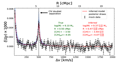
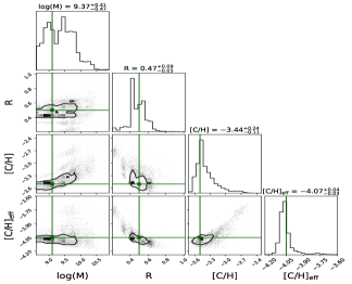
Figure 13: Correlation function measured from our mock dataset (left) and the inference results (right). The mock dataset is characterized by 20 QSO spectra, each with a C iv pathlength of $dz=1.0$, FHWM = 10 km/s, and SNR/pix = 50. Also plotted in the correlation function plot are fifty random draws (thin blue lines) and the mean inferred model (red line and red text) from the MCMC posterior distribution. The effective metallicity [C/H]_eff for the true model is calculated according to Eqn (3). The right panel shows the corner plot from MCMC sampling, where the true models are indicated by the green markers and lines. Note that the corner plot for [C/H]_eff is indirectly derived from the MCMC outputs of the other parameters (see text). The inferred parameters shown on the top of the corner plots represent the median and the 68% credible intervals. For this IGM model, we expect to simultaneously measure the values of log$\,M_{\rm{min}}$ to a precision of $\sim 0.44$ dex, [C/H] to a precision of $\sim 0.2$ dex, and $R$ to within $\sim 15\%$. The effective metallicity can be constrained indirectly within less than 0.05 dex.

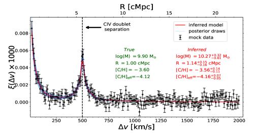
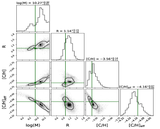
Figure 14: Same as Figure 13 but for a different IGM model with larger log$\,M$ and $R$ and smaller [C/H]. We find comparable precisions as Figure 13, where assuming our mock dataset, log$\,M_{\rm{min}}$ is measured to within $\sim 0.45$ dex, [C/H] to within 0.125 dex, and $R$ to within 13.5% at 1$\sigma$. The effective metallicity is indirectly constrained to less than 0.1 dex.

Finally, it is worth asking what upper limit we can set on the IGM metallicity in case of a null detection of the correlation function. We estimate the upper limit by restricting to models with a uniformly-enriched IGM. In this case, the inference problem now becomes one-dimensional with [C/H] being the only parameter. Assuming a flat prior and randomly choosing a mock dataset among our 10⁶ realizations, we compute the posterior numerically for a model with [C/H] = $-5.0$ and obtain an upper limit of [C/H] $<-4.35$ at 95% confidence.

4 Discussions and conclusions

We investigate the correlation function of the C iv forest as a probe of IGM metallicity and enrichment topology. We generate models of inhomogeneous enrichment using the halo catalogs from the $z=4.5$ snapshot of the Nyx hydrodynamic simulation, whereby halos above a minimum mass log$\,M_{\rm{min}}$ enrich their environments to a constant metallicity [C/H] out to a maximum radius $R$. We simulate the $z=4.5$ C iv forest with the Nyx simulation and compute the ionization fraction of C iv using CLOUDY. Skewers of the C iv forest are computed for each inhomogeneous enrichment model by interpolating CLOUDY ionization fraction outputs based on Nyx density and temperature fields.

The two-point correlation function (2PCF) of the C iv forest skewers has a clear peak at $dv=498$ km/s due to the doublet separation of the C iv absorption line. The amplitude of this peak increases quadratically with metallicity. The enrichment morphology parameters affect both the shape and amplitude of the 2PCF, where increasing log$\,M_{\rm{min}}$ and $R$ individually leads to an increase in power at both large and small scales. Since different combinations of log$\,M_{\rm{min}}$ and $R$ give rise to different values of mass- and volume-filling factors, the effect of enrichment morphology can also framed in terms of the filling factors.

Measurements of the IGM enrichment topology remain sparse and poorly-constrained. Booth et al. (2012) concluded that $f_{V}>0.1$ and $f_{m}>0.5$ are required to match the observed median C iv optical depth as a function of $\tau_{\mathrm{HI}}$ at $z=3$, which are satisfied when the IGM is predominantly enriched by low-mass ($<10^{10}M_{\odot}$) galaxies out to $r\geq 100$ proper kpc. The importance of low-mass galaxies for enriching the IGM is also found by other theoretical studies (e.g. Samui et al., 2008; Oppenheimer et al., 2009; Wiersma et al., 2010). On the other hand, by computing the clustering of discrete absorbers at the same redshift ($z=3$), Scannapieco et al. (2006) instead found that high-mass ($\approx 10^{12}M_{\odot}$) galaxies are mainly responsible for IGM enrichment out to $r\geq 500$ proper kpc. We estimate the precision to which the IGM metallicity and enrichment topology can be inferred using mock observations of 20 quasar spectra, where each spectrum is convolved to a resolution of FHWM = 10 km/s (equivalent to $R$=30,000 of Keck/HIRES or VLT/UVES) and has a SNR/pix = 50, for a total pathlength of $\Delta z$ = 20. The two IGM models shown in Figure 13 and Figure 14 are consistent with the best-fit model of Booth et al. (2012), although note that their work is at a much lower redshift than ours. We find that we can constrain the metallicity to a precision of $\sim 0.2$ dex at 1$\sigma$, while log$\,M_{\rm{min}}$ and $R$ can be constrained to within $\sim 0.4$ dex and $\sim 15\%$, respectively. Not only is our method different than those employed in existing studies, it is currently the state-of-the-art in simultaneously constraining the IGM metallicity and enrichment topology to high precision. We plan to apply our correlation function method to a real dataset in future work in the hope of potentially alleviating this disagreement.

We discuss how CGM absorbers near galaxies can bias clustering measurements of IGM absorbers, and investigate their effects by modeling their abundance based on observational constraints and injecting them into our mock spectra. We propose methods based on the flux PDF that can effectively remove CGM absorbers. While the flux distribution of IGM absorbers peaks at small $1-F$ values of $0.003-0.004$ and exponentially drops off at large values, the flux distribution of CGM absorbers remains mostly flat within the overlapping region. Depending on the IGM model, the IGM absorbers dominate over CGM absorbers by $\sim 20\%$ to a factor of a few tens at the peak. For a plausible IGM model with (log$\,M_{\rm{min}}$, $R$, [C/H]) = (9.50 $M_{\odot}$, 0.80 cMpc, $-3.50$) corresponding to ($f_{V}$, $f_{m}$, [C/H]_eff) = (0.12, 0.34, $-3.97$), IGM absorbers are $\sim 7-8$ times more abundant. While IGM absorbers dominate even more in models with higher filling fractions, up to $\sim 80$ times for a uniformly-enriched IGM with [C/H] = $-3.50$, CGM absorbers start to become comparable with IGM absorbers for models with ($f_{V}$, $f_{m}$) = (0.001, 0.05) and lower. Due to the distinct shapes of the IGM vs. CGM flux PDFs, we can remove CGM absorbers using a simple flux threshold. We also investigate an additional filtering scheme that automatically identifies CGM absorbers using their significance or $\chi$ field, whereby large $\chi$ values are attributed to CGM absorbers. By combining the flux threshold cutoff with a $\chi$ cutoff (including masking pixels around each extrema of the doublet), we can effectively mask out CGM absorbers and easily recover the underlying IGM correlation function from the masked spectra, since the correlation function is not affected by gaps in the spectra due to masking (as opposed to the power spectrum).

Another method to differentiate CGM from IGM absorbers is to perform a cut based on gas density. The gas density is related analytically to absorption in the Ly$\alpha$ forest, so Ly$\alpha$ forest absorption can be used as a proxy for density in real observations. In practice, since column density is an observable while density is not, it is easier to mask based on H i column density, where high H i column densities ($N_{\text{H\,{i}}}>10^{14}$ cm^-2) would likely correspond to CGM absorbers. One can also consider cross-correlating the Ly$\alpha$ forest with the C iv forest. In this work, we focus on the autocorrelation of the C iv forest as a probe of the background IGM metallicity and ignore how metallicity varies as a function of gas density. Cross-correlating the Ly$\alpha$ forest with the C iv forest connects the gas metallicity with the gas density and provides a more detailed picture of the IGM enrichment. This is motivationally similar to the pixel optical depth (POD) method that maps out the optical depth of metals as a function of the H i optical depth. The difference is that while the POD method measures this relation at zero velocity lag, i.e. in the same gas that gives rise to both the H i and metals, cross-correlation allows one to map out the relation over all velocity lags, thereby giving one more handle on the enrichment topology.

We did not consider foreground metal-line contamination in this work. Being one of the reddest metal lines and compared to bluer lines, C iv does not suffer from significant foreground contamination. However, lower redshift redder lines such as Fe ii $\lambda 1608$Å and Mg ii $\lambda 2796$Å and $\lambda 2804$Å lines can enter the C iv forest window and contaminate the resulting signal. Drawing inspiration from how Ly$\alpha$ forest cosmology handles metal line contamination (e.g., McDonald et al., 2006; Palanque-Delabrouille et al., 2013), one can first define wavelength windows that are redder than the C iv line, measure the correlation function within these windows using lower-redshift quasars, and finally subtract the measured correlation function from the higher-redshift C iv forest correlation function. Conventional methods of identifying individual lines, e.g. exploiting the separation of a foreground metal doublet and searching for additional transitions at the same redshift of the first metal line (Lidz et al., 2010), can also be applied to individual spectra to remove foreground contamination.

The auto-correlation of the metal-line forest presents a new avenue to constrain the enrichment history of the IGM, providing precise and simultaneous constraints on the IGM metallicity and enrichment topology. In a future work, we plan to apply this method to a sample of archival echelle quasar spectra. Viewed along current constraints obtained with existing methods such as the pixel optical depth method and standard Voigt profile fitting, this future measurement will shed light on the background IGM metallicity and cosmic enrichment history. There is also the possibility to extend the measurement to higher redshifts and investigate the evolution in the IGM metallicity. Higher-redshift measurements will be more challenging due to the decreasing metallicity and decreasing telescope sensitivity in the NIR (e.g., at $z=6$, the C iv forest redshifts into the $Y$ band), so having a larger quasar sample and more sensitive space-based observations (e.g. with JWST) is ideal. Application of the method to other metal species provides complementary constraints on other aspects of IGM physics. For instance, clustering of the Mg ii forest allows one to constrain the neutral hydrogen fraction during reionization H2020. Through measurements at different redshifts that probe the appearance of low-ions and the concurrent disappearance of high-ions with increasing redshift, it might be possible to observe the phase transition in the IGM due to reionization (Oh, 2002) as well as to constrain the relative abundance of these ions (e.g. Cooper et al., 2019; Becker et al., 2009).

Appendix A

In §3.2.3, we assess the efficiency of masking CGM absorbers on skewers with a random noise of SNR/pix = 50. Here we repeat the masking procedures on lower SNR data, one with SNR/pix = 20. Figure 15 shows the resultant $1-F$ and $\chi$ PDFs, where the cutoff thresholds represented by dashed black lines are placed at where each PDF starts plateauing, $1-F>0.15$ and $\chi>4$. The correlation function of the masked skewers is compared against the true IGM correlation function in Figure 16, where it is apparent that the correlation function of the masked skewers is significantly biased. Figure 17 shows that by using more aggressive masking thresholds that are placed at the magenta vertical lines in Figure 15 (where $1-F>0.06$ and $\chi>3$), one is able to recover the true IGM correlation function. The more aggressive flux + chi cut removes 38% of all pixels, compared to 29% from using the less aggressive cut. Although masking out CGM absorbers is more challenging with lower SNR data by requiring more aggressive masking (otherwise the results will be biased), we can include the values of the cuts in forward modeling and account for them in the inferencing.

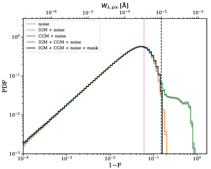
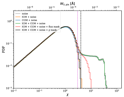
Figure 15: Same as Figure 11 and using the same IGM model, but with added Gaussian random noise resulting in SNR/pix = 20 instead. The cutoff thresholds indicated by the vertical black lines, located at $1-F=0.15$ and $\chi=4$, result in the masked correlation functions shown in Figure 16, while the more aggressive cutoffs indicated by the the vertical magenta lines, located at $1-F=0.06$ and $\chi=3$, give rise to the correlation functions shown in Figure 17.

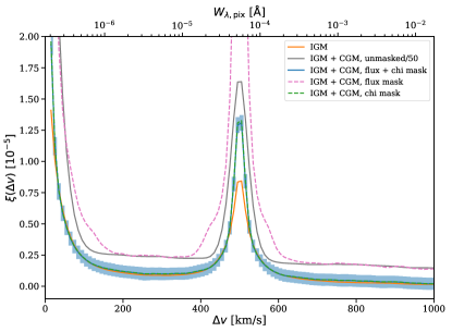
Figure 16: Comparison of the C iv forest correlation function before and after masking at the vertical black lines shown in Figure 15. Note that the unmasked IGM + CGM (gray) has been rescaled down by a factor of 50 to aid visualization. Flux masking alone results in a signicantly biased correlation function (dotted line), and residual bias remains even after combining the flux cut with a significance cut.

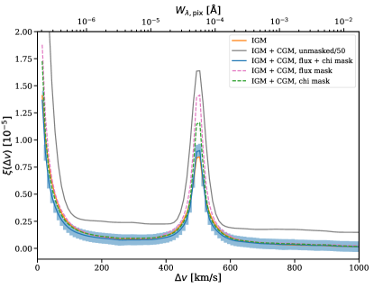
Figure 17: Same as Figure 16, but with cutoff thresholds indicated by the vertical magenta lines in Figure 15. The more aggressive masking is better able to recover the true IGM signal.

References

- Aguirre et al. (2001a) Aguirre A., Hernquist L., Schaye J., Weinberg D. H., Katz N., Gardner J., 2001a, ApJ, 560, 599
- Aguirre et al. (2001b) Aguirre A., Hernquist L., Schaye J., Katz N., Weinberg D. H., Gardner J., 2001b, ApJ, 561, 521
- Aguirre et al. (2002) Aguirre A., Schaye J., Theuns T., 2002, ApJ, 576, 1
- Aguirre et al. (2004) Aguirre A., Schaye J., Kim T.-S., Theuns T., Rauch M., Sargent W. L. W., 2004, ApJ, 602, 38
- Aguirre et al. (2005) Aguirre A., Schaye J., Hernquist L., Kay S., Springel V., Theuns T., 2005, ApJL, 620, L13
- Aguirre et al. (2008) Aguirre A., Dow-Hygelund C., Schaye J., Theuns T., 2008, ApJ, 689, 851
- Almgren et al. (2013) Almgren A. S., Bell J. B., Lijewski M. J., Lukić Z., Van Andel E., 2013, ApJ, 765, 39
- Aracil et al. (2004) Aracil B., Petitjean P., Pichon C., Bergeron J., 2004, AAP, 419, 811
- Asplund et al. (2009) Asplund M., Grevesse N., Sauval A. J., Scott P., 2009, ARA&A, 47, 481
- Astropy Collaboration et al. (2013) Astropy Collaboration et al., 2013, AAP, 558, A33
- Astropy Collaboration et al. (2018) Astropy Collaboration et al., 2018, AJ, 156, 123
- Bahcall & Peebles (1969) Bahcall J. N., Peebles P. J. E., 1969, ApJL, 156, L7
- Bautista et al. (2017) Bautista J. E., et al., 2017, AAP, 603, A12
- Becker et al. (2009) Becker G. D., Rauch M., Sargent W. L. W., 2009, ApJ, 698, 1010
- Bergeron et al. (2002) Bergeron J., Aracil B., Petitjean P., Pichon C., 2002, AAP, 396, L11
- Blomqvist et al. (2018) Blomqvist M., et al., 2018, JCAP, 2018, 029
- Boksenberg & Sargent (2015) Boksenberg A., Sargent W. L. W., 2015, ApJS, 218, 7
- Boksenberg et al. (2003) Boksenberg A., Sargent W. L. W., Rauch M., 2003, arXiv e-prints, pp astro–ph/0307557
- Booth et al. (2012) Booth C. M., Schaye J., Delgado J. D., Dalla Vecchia C., 2012, MNRAS, 420, 1053
- Bosman et al. (2017) Bosman S. E. I., Becker G. D., Haehnelt M. G., Hewett P. C., McMahon R. G., Mortlock D. J., Simpson C., Venemans B. P., 2017, MNRAS, 470, 1919
- Carswell et al. (2002) Carswell B., Schaye J., Kim T.-S., 2002, ApJ, 578, 43
- Cen & Chisari (2011) Cen R., Chisari N. E., 2011, ApJ, 731, 11
- Cen & Ostriker (1999) Cen R., Ostriker J. P., 1999, ApJL, 519, L109
- Chen et al. (2017) Chen S.-F. S., et al., 2017, ApJ, 850, 188
- Codoreanu et al. (2018) Codoreanu A., Ryan-Weber E. V., García L. Á., Crighton N. H. M., Becker G., Pettini M., Madau P., Venemans B., 2018, MNRAS, 481, 4940
- Cooksey et al. (2010) Cooksey K. L., Thom C., Prochaska J. X., Chen H.-W., 2010, ApJ, 708, 868
- Cooksey et al. (2013) Cooksey K. L., Kao M. M., Simcoe R. A., O’Meara J. M., Prochaska J. X., 2013, ApJ, 763, 37
- Cooper et al. (2019) Cooper T. J., Simcoe R. A., Cooksey K. L., Bordoloi R., Miller D. R., Furesz G., Turner M. L., Bañados E., 2019, ApJ, 882, 77
- Cowie & Songaila (1998) Cowie L. L., Songaila A., 1998, Nature, 394, 44
- Cowie et al. (1995) Cowie L. L., Songaila A., Kim T.-S., Hu E. M., 1995, AJ, 109, 1522
- D’Odorico et al. (2013) D’Odorico V., et al., 2013, MNRAS, 435, 1198
- D’Odorico et al. (2016) D’Odorico V., et al., 2016, MNRAS, 463, 2690
- Davé et al. (1998) Davé R., Hellsten U., Hernquist L., Katz N., Weinberg D. H., 1998, ApJ, 509, 661
- Dekker et al. (2000) Dekker H., D’Odorico S., Kaufer A., Delabre B., Kotzlowski H., 2000, in Iye M., Moorwood A. F., eds, Society of Photo-Optical Instrumentation Engineers (SPIE) Conference Series Vol. 4008, Optical and IR Telescope Instrumentation and Detectors. pp 534–545
- Ellison et al. (2000) Ellison S. L., Songaila A., Schaye J., Pettini M., 2000, AJ, 120, 1175
- Faber et al. (2003) Faber S. M., et al., 2003, in Iye M., Moorwood A. F. M., eds, Society of Photo-Optical Instrumentation Engineers (SPIE) Conference Series Vol. 4841, Instrument Design and Performance for Optical/Infrared Ground-based Telescopes. pp 1657–1669
- Ferland et al. (2017) Ferland G. J., et al., 2017, RMXAA, 53, 385
- Foreman-Mackey et al. (2013) Foreman-Mackey D., Hogg D. W., Lang D., Goodman J., 2013, PASP, 125, 306
- Friesen et al. (2016) Friesen B., Almgren A., Lukić Z., Weber G., Morozov D., Beckner V., Day M., 2016, Computational Astrophysics and Cosmology, 3, 4
- Gontcho A Gontcho et al. (2018) Gontcho A Gontcho S., Miralda-Escudé J., Font-Ribera A., Blomqvist M., Busca N. G., Rich J., 2018, MNRAS, 480, 610
- Haardt & Madau (2012) Haardt F., Madau P., 2012, ApJ, 746, 125
- Haehnelt et al. (1996) Haehnelt M. G., Steinmetz M., Rauch M., 1996, ApJL, 465, L95
- Hahn & Abel (2011) Hahn O., Abel T., 2011, MNRAS, 415, 2101
- Hasan et al. (2020) Hasan F., et al., 2020, ApJ, 904, 44
- Hennawi et al. (2020) Hennawi J. F., Davies F. B., Wang F., Oñorbe J., 2020, arXiv e-prints, p. arXiv:2007.15747
- Howlett et al. (2012) Howlett C., Lewis A., Hall A., Challinor A., 2012, JCAP, 2012, 027
- Kacprzak & Churchill (2011) Kacprzak G. G., Churchill C. W., 2011, ApJL, 743, L34
- Keating et al. (2014) Keating L. C., Haehnelt M. G., Becker G. D., Bolton J. S., 2014, MNRAS, 438, 1820
- Kobayashi et al. (2007) Kobayashi C., Springel V., White S. D. M., 2007, MNRAS, 376, 1465
- Lehner et al. (2016) Lehner N., O’Meara J. M., Howk J. C., Prochaska J. X., Fumagalli M., 2016, ApJ, 833, 283
- Lekien & Marsden (2005) Lekien F., Marsden J., 2005, International Journal for Numerical Methods in Engineering, 63, 455
- Lewis et al. (2000) Lewis A., Challinor A., Lasenby A., 2000, ApJ, 538, 473
- Lidz et al. (2010) Lidz A., Faucher-Giguère C.-A., Dall’Aglio A., McQuinn M., Fechner C., Zaldarriaga M., Hernquist L., Dutta S., 2010, ApJ, 718, 199
- Lukić et al. (2015) Lukić Z., Stark C. W., Nugent P., White M., Meiksin A. A., Almgren A., 2015, MNRAS, 446, 3697
- Madau et al. (2001) Madau P., Ferrara A., Rees M. J., 2001, ApJ, 555, 92
- Martin et al. (2010) Martin C. L., Scannapieco E., Ellison S. L., Hennawi J. F., Djorgovski S. G., Fournier A. P., 2010, ApJ, 721, 174
- McDonald et al. (2006) McDonald P., et al., 2006, ApJS, 163, 80
- Oh (2002) Oh S. P., 2002, MNRAS, 336, 1021
- Oppenheimer & Davé (2006) Oppenheimer B. D., Davé R., 2006, MNRAS, 373, 1265
- Oppenheimer et al. (2009) Oppenheimer B. D., Davé R., Finlator K., 2009, MNRAS, 396, 729
- Palanque-Delabrouille et al. (2013) Palanque-Delabrouille N., et al., 2013, AAP, 559, A85
- Pèrez-Ràfols & Miralda-Escudé (2015) Pèrez-Ràfols I., Miralda-Escudé J., 2015, in Highlights of Spanish Astrophysics VIII. pp 292–297
- Petitjean & Bergeron (1994) Petitjean P., Bergeron J., 1994, AAP, 283, 759
- Pichon et al. (2003) Pichon C., Scannapieco E., Aracil B., Petitjean P., Aubert D., Bergeron J., Colombi S., 2003, ApJL, 597, L97
- Pieri (2014) Pieri M. M., 2014, MNRAS, 445, L104
- Pieri et al. (2006) Pieri M. M., Schaye J., Aguirre A., 2006, ApJ, 638, 45
- Pieri et al. (2010) Pieri M. M., Frank S., Mathur S., Weinberg D. H., York D. G., Oppenheimer B. D., 2010, ApJ, 716, 1084
- Planck Collaboration et al. (2020) Planck Collaboration et al., 2020, AAP, 641, A6
- Prochaska et al. (2017) Prochaska J. X., et al., 2017, ApJ, 837, 169
- Rauch et al. (1996) Rauch M., Sargent W. L. W., Womble D. S., Barlow T. A., 1996, ApJL, 467, L5
- Rauch et al. (1997) Rauch M., Haehnelt M. G., Steinmetz M., 1997, ApJ, 481, 601
- Ryan-Weber et al. (2006) Ryan-Weber E. V., Pettini M., Madau P., 2006, MNRAS, 371, L78
- Ryan-Weber et al. (2009) Ryan-Weber E. V., Pettini M., Madau P., Zych B. J., 2009, MNRAS, 395, 1476
- Samui et al. (2008) Samui S., Subramanian K., Srianand R., 2008, MNRAS, 385, 783
- Sargent et al. (1980) Sargent W. L. W., Young P. J., Boksenberg A., Tytler D., 1980, ApJS, 42, 41
- Scannapieco et al. (2003) Scannapieco E., Schneider R., Ferrara A., 2003, ApJ, 589, 35
- Scannapieco et al. (2006) Scannapieco E., Pichon C., Aracil B., Petitjean P., Thacker R. J., Pogosyan D., Bergeron J., Couchman H. M. P., 2006, MNRAS, 365, 615
- Schaye et al. (2000) Schaye J., Rauch M., Sargent W. L. W., Kim T.-S., 2000, ApJL, 541, L1
- Schaye et al. (2003) Schaye J., Aguirre A., Kim T.-S., Theuns T., Rauch M., Sargent W. L. W., 2003, ApJ, 596, 768
- Schaye et al. (2007) Schaye J., Carswell R. F., Kim T.-S., 2007, MNRAS, 379, 1169
- Simcoe (2006) Simcoe R. A., 2006, ApJ, 653, 977
- Simcoe (2011) Simcoe R. A., 2011, ApJ, 738, 159
- Simcoe et al. (2002) Simcoe R. A., Sargent W. L. W., Rauch M., 2002, ApJ, 578, 737
- Simcoe et al. (2004) Simcoe R. A., Sargent W. L. W., Rauch M., 2004, ApJ, 606, 92
- Simcoe et al. (2011) Simcoe R. A., et al., 2011, ApJ, 743, 21
- Simcoe et al. (2013) Simcoe R. A., et al., 2013, PASP, 125, 270
- Songaila (1997) Songaila A., 1997, ApJL, 490, L1
- Songaila (2001) Songaila A., 2001, ApJL, 561, L153
- Songaila (2005) Songaila A., 2005, AJ, 130, 1996
- Songaila & Cowie (1996) Songaila A., Cowie L. L., 1996, AJ, 112, 335
- Sorini et al. (2018) Sorini D., Oñorbe J., Hennawi J. F., Lukić Z., 2018, ApJ, 859, 125
- Steidel (1990) Steidel C. C., 1990, ApJS, 72, 1
- Theuns et al. (2002) Theuns T., Viel M., Kay S., Schaye J., Carswell R. F., Tzanavaris P., 2002, ApJL, 578, L5
- Vernet et al. (2011) Vernet J., et al., 2011, AAP, 536, A105
- Virtanen et al. (2020) Virtanen P., et al., 2020, Nature Methods, 17, 261
- Vogt et al. (1994) Vogt S. S., et al., 1994, in Crawford D. L., Craine E. R., eds, Vol. 2198, Instrumentation in Astronomy VIII. SPIE, pp 362 – 375
- Walker (2019) Walker P. A., 2019, arXiv e-prints, p. arXiv:1904.09869
- Wiersma et al. (2010) Wiersma R. P. C., Schaye J., Dalla Vecchia C., Booth C. M., Theuns T., Aguirre A., 2010, MNRAS, 409, 132
- Wotta et al. (2016) Wotta C. B., Lehner N., Howk J. C., O’Meara J. M., Prochaska J. X., 2016, ApJ, 831, 95
- Zhu & Ménard (2013) Zhu G., Ménard B., 2013, ApJ, 770, 130
- Zhu et al. (2014) Zhu G., et al., 2014, MNRAS, 439, 3139
- du Mas des Bourboux et al. (2017) du Mas des Bourboux H., et al., 2017, AAP, 608, A130
- du Mas des Bourboux et al. (2019) du Mas des Bourboux H., et al., 2019, ApJ, 878, 47
- du Mas des Bourboux et al. (2020) du Mas des Bourboux H., et al., 2020, ApJ, 901, 153