A Latent Class Modeling Approach for Generating Synthetic Data and Making Posterior Inferences from Differentially Private Counts

Abstract

Several algorithms exist for creating differentially private counts from contingency tables, such as two-way or three-way marginal counts. The resulting noisy counts generally do not correspond to a coherent contingency table, so that some post-processing step is needed if one wants the released counts to correspond to a coherent contingency table. We present a latent class modeling approach for post-processing differentially private marginal counts that can be used (i) to create differentially private synthetic data from the set of marginal counts, and (ii) to enable posterior inferences about the confidential counts. We illustrate the approach using a subset of the 2016 American Community Survey Public Use Microdata Sets and the 2004 National Long Term Care Survey.

1 Introduction

National statistical organizations and other data curators, henceforth all called agencies, often seek to share collected information with outside researchers. Doing so requires methods that provide privacy protection to data subjects while maintaining statistical relationships in the data. Many agencies use statistical disclosure control (SDC) methods that blur the private data in a prescribed way, with the aim to provide some level of privacy protection. Traditional SDC methods include data swapping, cell suppression, top- or bottom- coding, and the addition of random noise (Hundepool et al., 2012). Generally, traditional SDC techniques have been applied with low intensity, so as not to degrade the quality of the information in the data. However, with the growth in available data and powerful computing, many agencies have become concerned that such SDC methods are not adequately protective.

To address this issue, several agencies have turned to using synthetic data methods (Rubin, 1993; Little, 1993; Reiter, 2005a). The agency releases data that are generated from some statistical model, estimated with the private data. With a full synthesis, agencies can ensure that no sensitive values are released on the file, which can reduce disclosure risks. Further, the agency can offer researchers access to record-level data instead of only summary statistics or other high-level information. Many different methods have been proposed to generate synthetic data (e.g., Reiter, 2005b; Woodcock and Benedetto, 2009; Mateo-Sanz et al., 2004; Slavković and Lee, 2010) and assess the utility and disclosure risk associated with the data release (Drechsler, 2011; Hundepool et al., 2012; Karr et al., 2006; Reiter et al., 2014; Snoke et al., 2018). The U.S. Census Bureau has released synthetic data for the Longitudinal Business Database (Kinney et al., 2011), Survey of Income and Program Participation (Benedetto et al., 2013), and the LEHD Origin-Destination Employment Statistics (with the data product being known as OnTheMap) (Machanavajjhala et al., 2008). Affiliated researchers have proposed methodologies for other national surveys (e.g., federal administrative data from the Office of Personnel Management (Barrientos et al., 2018)), and other statistical agencies have developed synthetic data products such as the Scottish Longitudinal Survey (SLS-DSU, 2018) and the German IAB Establishment Data (Drechsler, 2009).

Most SDC methods, including many synthetic data techniques, do not provide formally quantifiable privacy guarantees. Instead, agencies evaluate disclosure risks based on assumptions of intruder knowledge and behavior (Hundepool et al., 2012). An alternative approach is to design and use SDC methods that satisfy differential privacy (Dwork et al., 2006b). Differentially private algorithms exist for releasing counts (e.g., Dwork et al., 2006b; Ghosh et al., 2012), $k$-way marginals (Barak et al., 2007; Yang et al., 2012; Li et al., 2018), regression coefficients (Zhang et al., 2012; Snoke and Slavković, 2018; Awan and Slavkovic, 2021), and many other quantities that can be viewed as answers to user-specified queries. Several statistical agencies are interested in combining the privacy guarantees from differential privacy with the flexibility afforded by synthetic data. For example, the U.S. Census Bureau uses differentially-private synthetic data as the backbone of its 2020 population census data releases (Abowd, 2018). However, it can be challenging to generate differentially private synthetic data with low error (Garfinkel et al., 2018).

In this article, we propose methodology to generate differentially private synthetic data sets for multivariate count data, i.e., data from contingency tables. Our approach can be viewed as a post-processing method for generating synthetic data, a strategy also suggested in McKenna et al. (2021a). Specifically, we first assume that an agency has selected a set of marginal counts and has used some existing differentially private algorithm to add noise to those counts. For example, the agency could select the margins for which accurate values are especially important. Alternatively, the agency could select a set of margins that covers many types of analyses done by users of the data, e.g., all $k$-way margins. Second, we specify a Bayesian latent class model for the underlying confidential data (Dunson and Xing, 2009). We write the agency-selected margins as functions of the model parameters. Third, we estimate the parameters in the functions using only the differentially private counts and a composite likelihood-based approach (Lindsay, 1988). Finally, we sample from the estimated model to generate record-level, synthetic data. Agencies can generate multiple copies of the synthetic datasets, without any extra privacy loss, in order to enable secondary data analysts to estimate uncertainty and make inferences (Reiter, 2003). Generating differentially-private synthetic data from a user-specified list of summaries can be particularly advantageous for contingency tables with complex structures, e.g., data with structural zeros (Manrique-Vallier and Reiter, 2014; Li et al., 2018) or nested data such as individuals in households (Hu et al., 2018). We illustrate the latter in the online supplementary material.

The latent class modeling approach also can be viewed as an engine for approximate posterior inferences for the underlying confidential counts given a collection of differentially private counts, under the assumptions implied by the latent class model. Specifically, analysts can use parameters draws from the Markov chain Monte Carlo (MCMC) sampler to obtain posterior inferences for any functional of the parameters, i.e., any count in the table.

The remainder of the paper is organized as follows. In Section 1.1 we review related literature. In Section 2 we present preliminary information on data privacy and latent class models. In Section 3 we discuss the proposed approach and implementation details. In Section 4, we illustrate the approach by making posterior inferences from differentially private counts with a small set of variables from the 2016 American Community Survey (ACS) Public Use Microdata Sets (PUMS), and compare it to several other approaches from the literature. In Section 5, we illustrate the approach for both posterior inference and synthetic data generation using the 2004 National Long Term Care Survey, which has larger dimensions than the ACS example. For both illustrations, we use the Geometric Mechanism (Ghosh et al., 2012) to ensure differential privacy in the first stage counts. Finally, in Section 6 we end with a discussion.

1.1 Related Literature

Protection of counts and contingency tables has been the subject of many papers in the privacy literature. Some of the first examples of differentially-private (DP) data were counts and histograms perturbed by the Laplace mechanism (Dwork et al., 2006b). Barak et al. (2007) proposed methodology to produce DP marginal counts by using Fourier bases. Yang et al. (2012) extended this work to multi-dimensional contingency tables and noted some theoretical and practical shortcomings to both approaches. Machanavajjhala et al. (2008) proposed constructing DP contingency tables via a Dirichlet-Multinomial synthesizer, and the Hardt-Ligett-McSherry algorithm (Hardt et al., 2012) used a multiplicative weights approach.

Park and Ghosh (2014) proposed methodology for synthesis of DP contingency tables by disintegrating the data into suitable building blocks, injecting noise to these blocks, and using a Gibbs sampler to draw synthetic samples. Li et al. (2018) proposed to generate synthetic data by constructing an empirical hashed conditional distribution from the whole histogram and applying a Stability Based Algorithm to these empirical distributions. McKenna et al. (2019) proposed constructing DP synthetic data where “suitable building blocks” are a set of selected marginal counts; they add Laplace noise to the selected counts, fit a graphical model to the perturbed counts, and sample synthetic data from this model. Similarly, PrivBayes (Zhang et al., 2017) constructs DP synthetic data sets via Bayesian networks. These authors use networks to approximate the underlying data distribution through lower order marginals, add noise to these marginals, and approximate a full data distribution through the noisy counts and constructed Bayesian network. We note that these two methods placed first (McKenna et al., 2021b) and third (Bao et al., 2021), respectively, in the 2018-2019 National Institute of Standards and Technology Public Safety Communications Research division’s Differential Privacy Synthetic Data Challenge (National Institute of Standards and Technology, 2021); see Bowen and Snoke (2019) for a discussion of the performance of these methods in the context of the challenge. Similarly, the CIPHER method (Eugenio and Liu, 2018) estimates the joint distribution of a table based on a lower-order set of DP marginals. Their approach can be viewed as a post-processing technique for generating synthetic data.

Hay et al. (2010) showed that accuracy can be greatly improved by accounting for the constraints that a contingency table must satisfy in post-processing steps, although some very recent papers argue for post-processing to be part of posterior modeling (e.g., see Seeman et al. (2020), and references therin). Lee et al. (2015) extended this result by also accounting for the noise distribution and developed a fast generic approach for solving the resulting optimization problem.

Bowen and Liu (2016) compared many parametric and nonparametric methods for differentially private data synthesis, beyond those discussed above, and Charest (2012) showed that requiring greater privacy can degrade inferential results. Rinott et al. (2018) discussed several issues related to contingency table release under differential privacy, including the potential effects of rounding and other post-processing steps. They compared several simple mechanisms and offered comments on utility in private data releases. Similarly, Raab (2019) discussed some practical limitations to contingency table protection under formal privacy guarantees and presented a new method to create differentially private contingency tables from a subset of marginals via the Laplace mechanism and iterative proportional fitting.

All of these methods (ours included) are subject to the results of Ullman and Vadhan (2020). They showed that, even in simple cases, it is impossible to construct a polynomial time differentially private algorithm that preserves all two-way marginals.

Accounting for the additional privacy-preserving noise in inference also has been discussed in the literature. Charest (2012) used a simple Bayesian model to account for noise added under the Beta-Binomial synthesizer. Karwa et al. (2015) accounted for noise by treating the original data as missing. As the resulting likelihoods are often intractable, they developed a technique relying on a variational approximation for estimation. Seeman et al. (2020) showed that naive post-processing (such as direct modification of counts to meet constraints) can result in loss of information and proposed a Bayesian sampling scheme to post-process counts based on the noisy counts and outside constraining information. Gong (2019) showed that approximate Bayesian computing can be used to account for DP noise to obtain draws from the correct posterior distribution. Karwa et al. (2017) investigated methods to release DP synthetic networks while also accounting for the additional noise by treating the original private data as missing and using a likelihood-based approach. While not dealing with DP tables, Woo and Slavković (2012) proposed several EM algorithms to obtain correct logistic regression estimates for tables that are protected using the Post Randomization Method (PRAM) which could be extended to DP settings.

Turning to latent class models, Si and Reiter (2013) used latent class specifications for missing data imputation in contingency tables of Dunson and Xing (2009). This latent specification belongs to the family of Bayesian nonparametric techniques, which are well-known for being a flexible modeling choice to capture complex data patterns. Manrique-Vallier and Reiter (2014) refined these latent class models to incorporate cases with structural zeros, e.g., a person age five cannot have a college degree. The full table latent class approach was further extended to handle nested variables (e.g., individuals nested in households) (Hu et al., 2018), structural zeros (Akande et al., 2019a), and missing data (Akande et al., 2019b); see the Supplementary Material for a discussion of the model presented in Hu et al. (2018) and how our proposed approach can be augmented for nested data structures.

2 Preliminaries

2.1 Data Privacy Methods

2.1.1 Synthetic Data

Let $\mathbf{X}=\{(x_{i1},\dots,x_{ip})\}_{i=1}^{n}$ be an observed data set comprising $n$ individuals measured on $p$ confidential categorical variables. For $i=1,\dots,n$ and $j=1,\dots,p$, each $x_{ij}\in\{1,\dots,d_{j}\}$. We refer to the variables in $\mathbf{X}$ using $X_{j}$ where $j=1,\dots,p$. Synthetic data approaches aim to preserve the joint distribution $f(\mathbf{X})$ of these variables by modeling them simultaneously, e.g., as in Hu et al. (2018) and Akande et al. (2019b), or by using sequential modeling of the form,

$$f(\mathbf{X})=f(X_{1})f(X_{2}|X_{1})\cdots f(X_{p}|X_{1},\dots,X_{p-1}).$$ (1)

Different types of statistical models can be used for the conditional distributions in (1), including classification and regression trees (CART) (Reiter, 2005b), random forests (Caiola and Reiter, 2010), kernel density estimators (Woodcock and Benedetto, 2009), and combinations thereof (Barrientos et al., 2018). Choice of model depends on both the data structure and desired privacy levels.

2.1.2 Differential Privacy

Differential privacy (DP, (Dwork et al., 2006b, 2014)) is a formal privacy framework that gaurantees privacy protection by bounding the ratio of output densities for all neighboring data sets. Intuitively, it protects against attackers seeking to learn whether or not any specific individual’s data were included (or excluded) in the data set over which the output was calculated. That is, the inclusion (or exclusion) of a single person’s information does not change the output of the algorithm greatly. In this paper we focus on its strongest form, $\epsilon$-DP, where $\epsilon$ is a privacy-loss parameter, with smaller values indicating stronger protection, but our model could be modified for other forms of DP.

Definition 2.1.

$\epsilon$-Differential Privacy (Dwork et al., 2006b): A randomized algorithm $\mathcal{A}$ satisfies $\epsilon$-differential privacy if for all data sets $\mathbf{X}=\{(x_{i1},\dots,x_{ip})\}_{i=1}^{n}$ and $\mathbf{X^{\prime}}$ differing on at most one row, and $\mathcal{S}\subseteq\mathrm{Range}(\mathcal{A})$,

$$\frac{\mathrm{Pr}[\mathcal{A}(\mathbf{X})\in S]}{\mathrm{Pr}[{\mathcal{A}(\mathbf{X^{\prime}})}\in S]}\leq\exp(\epsilon)\,.$$ (2)

Differential privacy is a property of the algorithm itself. It is achieved by randomness. Many different algorithms have been proposed to release differentially private statistics or data sets (e.g., the Laplace (Dwork et al., 2006b) or Geometric (Ghosh et al., 2012) mechanisms, which are the most relevant to our seeting). Several relaxations and extensions of differential privacy have been proposed such as $(\epsilon,\delta)$-differential privacy (Dwork et al., 2006a) and Rényi differential privacy (Mironov, 2017); for more, see Dwork et al. (2014).

Many DP mechanisms (ours included) rely on the useful properties of post-processing and sequential composition. These properties outline how DP privacy guarantee can be preserved and how the privacy-loss parameter is propagated through multiple data releases. Theorem 2.2 shows that DP is preserved through post-processing, and is key to our proposed approach: the augmented Bayesian latent class model and measurement error model is a post-processing technique for a noisy, privacy-preserving count. Theorem 2.3 shows how the privacy-loss parameter $\epsilon$ propagates through multiple data releases on the same individual.

Theorem 2.2.

Post-processing (Dwork et al., 2006b): Let $\mathcal{A}$ be any randomized algorithm such that $\mathcal{A}(\mathbf{X})$ is $\epsilon$-differentially private, and let $g$ be any function. Then, $g(\mathcal{A}(\mathbf{X}))$ also satisfies $\epsilon$-differential privacy.

Theorem 2.3.

Sequential composition (McSherry, 2009): Let $\mathcal{A}_{i}$ each provide $\epsilon_{i}$-differential privacy. The sequence of $\mathcal{A}_{i}(\mathbf{X})$ provides $(\sum_{i}\epsilon_{i})$-differential privacy.

2.1.3 Geometric Mechanism

The Geometric Mechanism (Ghosh et al., 2012) adds noise from a two-sided geometric distribution to achieve differential privacy. Properties of this distribution, including simulation techniques, are discussed in Inusah and Kozubowski (2006) and its references.

Definition 2.4.

A random variable $Y$ distributed as a two-sided geometric distribution has probability mass function

$$P(Y=k)=\frac{1-\alpha}{1+\alpha}\alpha^{|k|}$$ (3)

where $0\leq\alpha\leq 1$.

Theorem 2.5.

Geometric Mechanism (Ghosh et al., 2012): For $f:\mathcal{D}\rightarrow\mathbf{R}^{d}$, the mechanism $\mathcal{A}$ that adds independently drawn noise from a $\mathrm{two}$-$\mathrm{sided}$-$\mathrm{Geom}(\exp\{\frac{-\epsilon}{\Delta f}\})$ distribution to each of the $d$ terms of satisfies $\epsilon$-differential privacy.

This mechanism has several appealing properties for protecting count data. First, the added noise values are integers, which eliminates the need for a post-processing step to deal with decimals. Second, Ghosh et al. (2012) show that this mechanism is optimal for every potential user regardless of the side information that they posses when releasing DP count queries using a Bayesian framework.

2.2 Bayesian Latent Class Models

Dunson and Xing (2009) developed a flexible methodology for modeling unordered categorical data using a Bayesian nonparametric mixture model. Their methods are directly applicable to modeling complete contingency tables.

Suppose each observation $i=1,\dots,n$ belongs to a latent class denoted by $z_{i}\in\{1,2,\dots\}$. The probability for each unique combination of variable levels is specified according to these latent classes. For ease of notation, we allow $x_{ij}$ to stand for random variables as well as the observed data. The latent class model is of the form,

$$\begin{split}x_{ij}|z_{i},\{\Psi_{h}^{(j)}\}_{h=1}^{\infty}&\stackrel{{\scriptstyle ind}}{{\sim}}Multinomial\{1,\Psi_{z_{i}1}^{(j)},\dots,\Psi_{z_{i}d_{j}}^{(j)}\},i=1,\dots,n,\,j=1,\dots,p,\\ z_{i}|\{\pi_{h}\}_{h=1}^{\infty}&\stackrel{{\scriptstyle ind}}{{\sim}}Discrete\{(1,\dots,\infty),(\pi_{1},\dots,\pi_{\infty})\},\\ \pi_{h}&=V_{h}\prod_{l<h}(1-V_{l}),\quad V_{h}\sim\beta(1,\alpha),\\ \Psi_{h}^{(j)}&\sim Dirichlet(a_{j1},\dots,a_{{jd}_{j}}),\\ \end{split}$$ (4)

where $\Psi_{h}^{(j)}=(\Psi_{h1}^{(j)},\dots,\Psi_{hd_{j}}^{(j)})$, $\alpha>0$, and $(a_{j1},\dots,a_{jdj})$ is a vector with positive components. Under model (4), for any feasible set of values $(c_{1},\dots,c_{p})$ of the categorical variables, one has

$$Pr(x_{i1}=c_{1},\dots,x_{ip}=c_{p}|\{\Psi_{h}^{(j)}\}_{h=1}^{\infty},\{\pi_{h}\}_{h=1}^{\infty})=\sum_{h=1}^{\infty}\pi_{h}\prod_{j=1}^{p}\Psi_{hc_{j}}^{(j)},\,$$ (5)

which corresponds to a mixture of product multinomials with a Dirichlet process (Ferguson, 1973) as a mixing distribution.

To facilitate posterior computation, we use a finite dimensional approximation of model (4), which can be estimated using Gibbs sampling. The approximation relies on the assumption that $z_{i}\in\{1,\dots,k\}$, where $k<\infty$, which is equivalent to truncating the mixture model (5) to $k$ components; see Ishwaran and James (2001) for a discussion of the truncated Dirichlet processes. Similar approximations along with Gibbs sampling have been successfully used for private data synthesis, including in Hu et al. (2018), Manrique-Vallier and Reiter (2014) and Akande et al. (2019b), among others.

2.3 Composite Likelihood Methods

Composite likelihood methods allow analysts to circumvent the specification of the full joint likelihood function (Lindsay, 1988; Varin et al., 2011). Instead, analysts can use an approximation to the likelihood function, often with the assumption of some form of independence, to simplify computation.

We use composite likelihood methods to approximate the joint likelihood of the latent class model given an agency-specified set of marginal counts. Let $(M_{1},\ldots,M_{T})$ represent the list of marginal counts of $\mathbf{X}$ with $\theta=\left(\{\Psi_{h}^{(j)}\}_{h=1,j=1}^{k,p},\,\{\pi_{h}\}_{h=1}^{k}\right)$. Let $\mathcal{L}_{t}(\theta;M_{t})$ be the likelihood function corresponding to $M_{t}$ induced by Model (4). We approximate the joint likelihood of $\theta$ given $(M_{1},\ldots,M_{T})$ using

$$\mathcal{L}_{C}(\theta;M_{1},\ldots,M_{T})\approx\prod_{t=1}^{T}\mathcal{L}_{t}(\theta;M_{t}).$$ (6)

The composite likelihood $\mathcal{L}_{C}$ allows for inference about $\theta$ only from the marginal counts (Varin et al., 2011). We note that, while computationally expedient, inference based on only a subset of counts of $\mathbf{X}$ could result in inaccurate estimates of $\theta$ (Walker, 2013), particularly for regions of its distribution that describe the counts excluded from the set of selected marginals. Furthermore, not all combinations of marginals, and possibly conditional distributions fully and uniquely specify the joint distribution (e.g., see Fienberg and Slavkovic (2005); Slavković et al. (2015) within the context of confidentiality protection, and more general related references therein).

3 Proposed Methods

3.1 Overview

We assume the agency adds noise to the true counts for a set of agency-specified marginals, $(M_{1},\ldots,M_{T})$, computed from $\mathbf{X}$ using the Geometric mechanism. In our simulation examples, we use the definition of sensitivity based on changing one row; hence, the sensitivity for each $M_{t}$, where $t=1,\ldots,T$, equals two. We assume the agency has determined appropriate values of $\epsilon$ to control the overall privacy budget. See Section 4 for a discussion in the context of our simulations.

When estimating the parameters of the Bayesian latent class model, we account for the additional noise due to DP using a measurement error model (Fuller, 2009). Specifically, we treat the true underlying counts as unknown and incorporate the privacy preserving mechanism into the model. Let $\mathbf{\tilde{M}}$ denote the observed noisy marginal counts. We have

$$\begin{split}\mathbf{\tilde{M}}&=(M_{1}+\varepsilon_{1},\ldots,M_{T}+\varepsilon_{T}),\\ \varepsilon_{t}&\overset{ind}{\sim}\mathrm{two}\mbox{-}\mathrm{sided}\mbox{-}\mathrm{Geom}_{r_{t}}\left(\exp\left\{\frac{-\epsilon}{\Delta M_{t}T}\right\}\right),t=1,\ldots,T,\\ M_{t}|\boldsymbol{\pi}_{k},\boldsymbol{\Psi}_{k}&\overset{ind}{\sim}{\rm Multinomial}_{r_{t}}(n,P_{t}(\boldsymbol{\pi}_{k},\boldsymbol{\Psi}_{k})),\;t=1,\ldots,T,\\ \boldsymbol{\pi}_{k}&=\{\pi_{h}\}_{h=1}^{k},\;\boldsymbol{\Psi}_{k}=\{\Psi_{h}^{(j)}\}_{h=1,j=1}^{k,p},\end{split}$$ (7)

where each $M_{t}$ comprises $r_{t}$ counts, $\varepsilon_{t}$ is a random vector with $r_{t}$ independent components distributed as $\mathrm{two}\mbox{-}\mathrm{sided}\mbox{-}\mathrm{Geom}\left(\exp\left\{\frac{-\epsilon}{\Delta M_{t}}\right\}\right)$, and ${\Delta M_{t}}=2$ is the sensitivity of $M_{t}$. We complete the model specification by assuming the prior distributions for $\boldsymbol{\pi}_{k}$ and $\boldsymbol{\Psi}_{k}$ used in (4). Since the summaries $M_{t}$ are assumed to be marginal counts, the distribution induced by $\mathbf{X}\mapsto M_{t}$ is multinomial with parameters $n$ and $P_{t}(\boldsymbol{\pi}_{k},\boldsymbol{\Psi}_{k})$, where $P_{t}(\boldsymbol{\pi}_{k},\boldsymbol{\Psi}_{k})$ represents the probabilities of the counts in $M_{t}$ and is computed using expression (5).

The third line of (7) represents our “augmented” step (Lindsay, 1988; Varin et al., 2011): each marginal count is assumed to be independently drawn from multinomial distributions. We rely on this assumption as it is not obvious how to characterize the joint distribution for $(M_{1},\ldots,M_{T})|\boldsymbol{\pi}_{k},\boldsymbol{\Psi}_{k}$. Although the premise of independence leads to a product of multinomial distributions that places positive probability outside the range of $(M_{1},\ldots,M_{T})$, we expect such probability to be small since $(P_{1}(\boldsymbol{\pi}_{k},\boldsymbol{\Psi}_{k}),\ldots,P_{T}(\boldsymbol{\pi}_{k},\boldsymbol{\Psi}_{k}))$ is a coherent system of probabilities that accounts for the underlying constraints among $M_{1},\ldots,M_{T}$. Hence, in order to generate synthetic tables that consider such constraints, our strategy is to sample from the distribution of $\boldsymbol{\pi}_{k},\boldsymbol{\Psi}_{k}|\boldsymbol{\tilde{M}}$, and approximate the underlying table cell probabilities by

$$Pr(x_{{(n+1)}1}=c_{1},\dots,x_{{(n+1)}p}=c_{p}|\boldsymbol{\tilde{M}})=$$

$$\int\int Pr(x_{{(n+1)}1}=c_{1},\dots,x_{{(n+1)}p}=c_{p}|\boldsymbol{\pi}_{k},\boldsymbol{\Psi}_{k})Pr(\boldsymbol{\pi}_{k},\boldsymbol{\Psi}_{k}|\boldsymbol{\tilde{M}})d\boldsymbol{\pi}_{k}d\boldsymbol{\Psi}_{k}.$$

Here, $Pr(x_{{(n+1)}1}=c_{1},\dots,x_{{(n+1)}p}=c_{p}|\boldsymbol{\pi}_{k},\boldsymbol{\Psi}_{k})$ is defined as in (5).

Regardless of which marginal counts are used in estimation, probabilities corresponding to any cell of the contingency table or marginal count can be estimated through ($\boldsymbol{\pi}_{k},\boldsymbol{\Psi}_{k}$). At each iterate, the desired probabilities can be tabulated using the sampled values of ($\boldsymbol{\pi}_{k},\boldsymbol{\Psi}_{k}$) at that iterate. This results in a posterior distribution for each desired probability. Synthetic data can be created from the full cell counts either by straightforward post-processing (e.g., multiply full table probabilities by the desired table size and expand) or by multinomial sampling of the cells weighted by the full table probabilities.

Any arbitrary set of summary statistics can be fed into the model. However, to increase the statistical usefulness of the estimated table, we suggest using sets of summary statistics that include at least one instance of every variable and its corresponding levels, which we do here. In addition, when privacy budgets are constrained, we recommend using few rather than many marginal counts. Using a smaller set of marginals allocates more of the privacy budget to each marginal table, which can improve accuracy for those counts. We note that the dimension of parameters ($\boldsymbol{\pi},\boldsymbol{\psi}$) to be estimated does not depend on the number of tables passed to the model.

In general, we expect these results to improve as the accuracy of the formally private counts improves. However, difficulties can arise with the measurement error step of our model if it is hard to specify the DP noise generating process.

This approach to differentially private synthesis does not suffer from privacy loss from running the estimation algorithm. Noise is injected to the marginal counts prior to the MCMC sampling (Chaudhuri et al., 2013). The algorithm uses these noisy marginals and knowledge of the noise distribution (which does not violate differential privacy) to estimate the underlying contingency table through ($\boldsymbol{\pi}_{k},\boldsymbol{\Psi}_{k})$.

3.2 Illustrative Implementation

To illustrate implementations, suppose the agency has generated all 40 two-way marginal counts from a $2^{5}$ table. We can write each two-way marginal probability as a sum over all combinations of the remaining three variables, for example,

$$\begin{split}Pr(x_{i1}=0,x_{i2}=0|\boldsymbol{\pi}_{k},\boldsymbol{\Psi}_{k})&=\sum_{j=0}^{1}\sum_{l=0}^{1}\sum_{m=0}^{1}Pr(x_{i1}=0,x_{i2}=0,x_{i3}=j,x_{i4}=l,x_{i5}=m|\boldsymbol{\pi}_{k},\boldsymbol{\Psi}_{k})\\ &=\sum_{h=1}^{k}\pi_{h}\Psi_{h0}^{(1)}\Psi_{h0}^{(2)}\sum_{j=0}^{1}\sum_{l=0}^{1}\sum_{m=0}^{1}\Psi_{hj}^{(3)}\Psi_{hl}^{(4)}\Psi_{hm}^{(5)}\,.\end{split}$$ (8)

Similarly, we have

$$\begin{split}Pr(x_{i1}=0,x_{i2}=1|\boldsymbol{\pi}_{k},\boldsymbol{\Psi}_{k})&=\sum_{h=1}^{k}\pi_{h}\Psi_{h0}^{(1)}\Psi_{h1}^{(2)}\sum_{j=0}^{1}\sum_{l=0}^{1}\sum_{m=0}^{1}\Psi_{hj}^{(3)}\Psi_{hl}^{(4)}\Psi_{hm}^{(5)}\\ Pr(x_{i1}=1,x_{i2}=0|\boldsymbol{\pi}_{k},\boldsymbol{\Psi}_{k})&=\sum_{h=1}^{k}\pi_{h}\Psi_{h1}^{(1)}\Psi_{h0}^{(2)}\sum_{j=0}^{1}\sum_{l=0}^{1}\sum_{m=0}^{1}\Psi_{hj}^{(3)}\Psi_{hl}^{(4)}\Psi_{hm}^{(5)}\\ Pr(x_{i1}=1,x_{i2}=1|\boldsymbol{\pi}_{k},\boldsymbol{\Psi}_{k})&=\sum_{h=1}^{k}\pi_{h}\Psi_{h1}^{(1)}\Psi_{h1}^{(2)}\sum_{j=0}^{1}\sum_{l=0}^{1}\sum_{m=0}^{1}\Psi_{hj}^{(3)}\Psi_{hl}^{(4)}\Psi_{hm}^{(5)}.\\ \end{split}$$ (9)

We denote the probabilities in (8) and (9) by $P_{t}(\boldsymbol{\pi}_{k},\boldsymbol{\Psi}_{k})$ for each corresponding count in Model 7.

After writing all the two-way marginal counts as functions of the latent class parameters, we can estimate the posterior distribution of all parameters using a MCMC sampler; see Supplementary Section 2 for details. We developed an R package to fit the proposed model given an arbitrary set of two-way marginals from a $2^{p}$ contingency table of any size

4 Application to American Community Survey Data

In this section, we illustrate the proposed approach using data from the ACS PUMS and a small number of variables; see Table 1. In this illustration, we use the latent class model as a post-processing algorithm to obtain posterior inferences from a set of released noisy counts.

4.1 Data Description

For each simulation run, we randomly select a subset of 10,000 individuals from the 2016 one-year ACS PUMS. We use five variables on each individual, namely sex, age, race, citizenship, and income. We recode the latter four variables to binary variables using the rules in Table 1. Table 2 displays all the 2-way marginal tables from one such sample, to give a sense of the typical counts.

Table 1: Data description for the ACS recoded variables. Original data was collected from the 2016 1-year ACS PUMS and recoded according to the guidelines below.

Variable	Label	Levels
Sex	SEX	0: males, 1: females
Age	AGE	0: under age 18, 1: over age 18
Race	RACE	0: non-white, 1: white
Citizenship	CIT	0: non-U.S. citizen, 1: U.S. citizen
Income	INC	0: income under federal poverty line
		1: income above federal poverty line

Table 2: All two-way marginal tables for one randomly sampled subset of 10,000 observations from the 2016 ACS PUMS.

	Age
Citizenship	0	1
0	11	596
1	443	8,950

	Race
Citizenship	0	1
0	299	308
1	1,731	7,662

	Sex
Citizenship	0	1
0	273	354
1	4,505	4,888

	Income
Citizenship	0	1
0	294	313
1	2,916	6,477

	Race
Age	0	1
0	110	344
1	1,920	7,626

	Sex
Age	0	1
0	239	215
1	4,539	5,007

	Income
Age	0	1
0	445	9
1	2,765	6,781

	Sex
Race	0	1
0	945	1,085
1	3,833	4,137

	Income
Race	0	1
0	827	1,203
1	2,382	5,587

	Income
Sex	0	1
0	1,281	3,497
1	1,929	3,293

4.2 Simulation Details

We base our example on the assumptions that the agency has decided that all two-way marginal tables are useful to the end data user and will create differentially private versions of them. To make the differentially private counts, we add independent noise drawn from the Geometric mechanism with $\epsilon\in\{0.25,0.5,1.0\}$. We invoke sequential composition theorems to adhere to the specified values of $\epsilon$. In particular, each of the 40 two-way marginal counts belongs to one of $5\choose 2$ $=10$ two-way tables. Thus, each individual contributes to only one cell per table but contributes across all ten tables. Accordingly, each marginal table should be perturbed with one-tenth of the privacy budget.

After generating the noisy counts in each simulation run, we use a MCMC sampler to iteratively sample the unknown parameters, $(M_{1},\ldots,M_{T},\boldsymbol{\pi}_{k},\boldsymbol{\Psi}_{k})$. Unless otherwise noted, we set the number of latent classes equal to $k=10$. In fitting, generally at least four classes have non-trivial mass (as determined by $\boldsymbol{\pi_{k}}$); see Supplementary Section 2 for model implementation details.

We run the algorithm for 5,000 iterations, discarding the first 2,000 iterations as burn-in. We monitor convergence of model probabilities using trace plots, a standard practice in Bayesian data analysis (Gelman et al., 2013; Roy, 2020). In each iteration, we compute the probabilities for all two-way margins and cells in the full table according to the latent class specification using the sampled parameters $(\boldsymbol{\pi}_{k},\boldsymbol{\Psi}_{k})$ at that iterate.

We compare outputs from the latent class model to output generated using PrivBayes (Zhang et al., 2017), following the architecture for adapting PrivBayes to private data releases described in Ping et al. (2017). To do so, we adapt their publicly-available Python code, accessible at https://github.com/DataResponsibly/DataSynthesizer. We also compare to a graphical model-based approach (McKenna et al., 2019) by adapting their publicly-available Python code, accessible at https://github.com/ryan112358/private-pgm. We chose these methods due to their prevalence, performance capabilities, and similarities to our proposed approach in terms of inputs in the sense that all comparison methods are created from marginal counts instead of the full, underlying table.

The codes for these two methods return different outputs. PrivBayes returns a synthetic data set, which we convert into probabilities for the full table. The graphical model-based approach returns a vector of numbers (not necessarily counts) summing to the sample size that corresponds to “counts” for each of the full table cells. We normalize these numbers to create probabilities for the full table. We note that, unlike our proposed latent class approach, neither of these methods generate uncertainty estimates.

4.3 Results

Before turning to the results using differentially private marginals, we first study the usefulness of the composite likelihood approach and the corresponding assumption of independent counts absent privacy concerns, i.e., with $\epsilon=\infty$.

4.3.1 Performance Absent Privacy Concerns

We estimate the augmented latent class model for the underlying table without adding privacy-preserving noise to the marginal counts. To do, we fit model (7) using the true $(M_{1},\dots,M_{T})$ and without the measurement error components in the first two lines of that model.

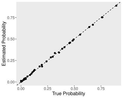
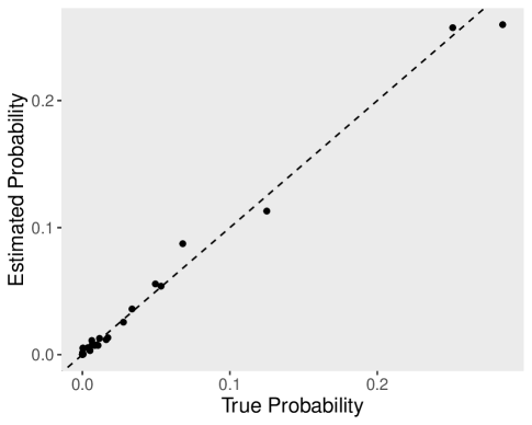
Figure 1: True versus estimated two-way marginal (top) and full table (bottom) probabilities for the ACS simulation with no noise added for privacy. True counts without added noise used as input. The number of latent classes set to 10. As two-way margins were used as inputs, we see more accurate estimation of the marginal probabilities. Accurate estimation of the full cell probabilities is not guaranteed, but can occur.

Figure 1 displays posterior modes from one run of the simulation for the marginal and full table probabilities. Results from additional runs are very similar. Both marginal and full cell probabilities are estimated accurately. The independence assumption appears to have minimal negative effects on estimation of the marginal probabilities, while also returning reasonable estimates for the full table cell probabilities. We note that this latter fact stems from the absence of strong three-way (and higher) interaction effects among the variables. In general, one should not expect accurate estimates for the full table; rather, one should expect accurate estimates of the marginal counts used in the estimation routines.

4.3.2 Performance with Noisy Counts

We next generate differentially-private counts and corresponding posterior inferences for the data described in Section 4.1, using the algorithm described in Section 3.

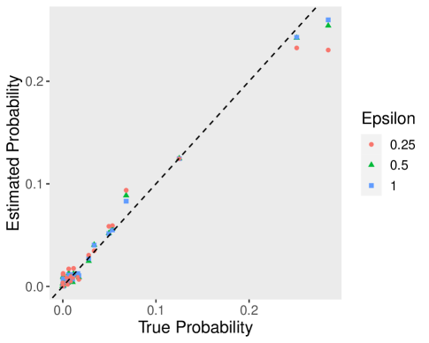
Figure 2: Plots of true marginal probabilities versus estimated marginal probabilities (top) and true full table probabilities versus estimated probabilities (bottom) for $\epsilon\in\{0.25,0.5,1.0$}. Estimated marginal probabilities denote the mean of the posterior distribution for the corresponding marginal probability. As expected, estimation accuracy visually increase as the $\epsilon$ grows.

Figure 2 displays posterior means for the estimated marginal and full cell probabilities modes from one run of the simulation. Results from additional runs are very similar. The results exhibit some expected trends. As the privacy loss budget $\epsilon$ increases, the amount of added noise decreases, resulting in better estimates of marginal and full cell probabilities. In the case of marginal probabilities, results for all values of the privacy loss budget return estimates that coincide well with the underlying probabilities, as shown in Figure 2. The results demonstrate this behavior for all values of $\epsilon$. For the full table probabilities, the proposed approach reasonably reconstructs the underlying probabilities even though full table counts are not used in estimation. In general, there is more variation from the truth when compared to the estimates of the marginal probabilities. This also corresponds with the privacy budget: lower values of $\epsilon$ display more disagreement from the true values compared to higher values. This is reasonable to expect as only the marginal counts were used directly in estimation.

We also conducted repeated simulations to assess how well the procedure captures the underlying marginal counts for each value of $\epsilon$. To do so, we repeat the entire procedure 100 times. Each time we sample 10,000 observations from the full original data, compute all two-way marginals, apply the Geometric Mechanism, and implement our method. For each marginal count, we examine the posterior distribution of the corresponding marginal probability and construct 95% credible intervals using the 2.5^th and 97.5^th quantiles of the posterior distribution. We record the coverage of the true probability, that is, whether or not the population count is inside the posterior interval.

Table 3: Coverage probabilities (“Cov.”)and average credible interval length (“Length”) for the forty two-way marginal counts.

		$\epsilon$ = 0.25		$\epsilon$ = 0.50		$\epsilon$ = 1.00		$\epsilon$ = $\infty$
Cell	Pop. Value	Cov.	Length	Cov.	Length	Cov.	Length	Cov.	Length
00…	$0.002$	$0.10$	$0.01$	$0.44$	$0.01$	$0.70$	$0.01$	$0.97$	$0.01$
01…	$0.061$	$0.97$	$0.04$	$1.00$	$0.03$	$1.00$	$0.02$	$1.00$	$0.02$
10…	$0.044$	$0.71$	$0.03$	$0.90$	$0.03$	$1.00$	$0.02$	$1.00$	$0.03$
11…	$0.894$	$0.49$	$0.05$	$0.89$	$0.04$	$0.99$	$0.03$	$1.00$	$0.04$
0.0..	$0.031$	$0.83$	$0.03$	$0.89$	$0.03$	$0.98$	$0.03$	$1.00$	$0.03$
0.1..	$0.031$	$0.16$	$0.04$	$0.37$	$0.03$	$0.74$	$0.02$	$0.92$	$0.02$
1.0..	$0.174$	$0.88$	$0.05$	$0.89$	$0.04$	$0.96$	$0.04$	$0.99$	$0.04$
1.1..	$0.763$	$0.57$	$0.06$	$0.79$	$0.05$	$0.95$	$0.04$	$0.97$	$0.04$
0..0.	$0.031$	$1.00$	$0.03$	$1.00$	$0.03$	$1.00$	$0.02$	$1.00$	$0.02$
0..1.	$0.031$	$0.98$	$0.03$	$1.00$	$0.03$	$1.00$	$0.02$	$1.00$	$0.02$
1..0.	$0.453$	$1.00$	$0.05$	$1.00$	$0.05$	$1.00$	$0.04$	$1.00$	$0.04$
1..1.	$0.485$	$0.99$	$0.05$	$1.00$	$0.05$	$1.00$	$0.04$	$1.00$	$0.04$
0…0	$0.027$	$1.00$	$0.03$	$1.00$	$0.03$	$1.00$	$0.03$	$1.00$	$0.03$
0…1	$0.035$	$0.88$	$0.03$	$0.98$	$0.03$	$1.00$	$0.02$	$1.00$	$0.02$
1…0	$0.298$	$1.00$	$0.06$	$1.00$	$0.05$	$1.00$	$0.05$	$1.00$	$0.06$
1…1	$0.640$	$0.98$	$0.06$	$1.00$	$0.06$	$1.00$	$0.05$	$1.00$	$0.06$
.00..	$0.011$	$0.94$	$0.02$	$0.96$	$0.02$	$1.00$	$0.02$	$1.00$	$0.02$
.01..	$0.035$	$0.77$	$0.03$	$0.95$	$0.03$	$1.00$	$0.02$	$1.00$	$0.03$
.10..	$0.195$	$0.99$	$0.05$	$1.00$	$0.04$	$1.00$	$0.04$	$1.00$	$0.04$
.11..	$0.759$	$0.89$	$0.06$	$0.97$	$0.05$	$0.99$	$0.04$	$1.00$	$0.05$
.0.0.	$0.024$	$0.95$	$0.03$	$1.00$	$0.02$	$1.00$	$0.02$	$1.00$	$0.02$
.0.1.	$0.022$	$0.78$	$0.03$	$0.84$	$0.03$	$0.93$	$0.02$	$1.00$	$0.02$
.1.0.	$0.461$	$1.00$	$0.05$	$1.00$	$0.05$	$1.00$	$0.04$	$1.00$	$0.05$
.1.1.	$0.493$	$0.98$	$0.05$	$0.99$	$0.05$	$1.00$	$0.04$	$1.00$	$0.05$
.0..0	$0.045$	$0.60$	$0.03$	$0.67$	$0.03$	$0.93$	$0.03$	$1.00$	$0.04$
.0..1	$0.001$	$0.00$	$0.03$	$0.00$	$0.02$	$0.00$	$0.02$	$0.00$	$0.02$
.1..0	$0.280$	$0.93$	$0.06$	$0.90$	$0.05$	$0.93$	$0.05$	$1.00$	$0.06$
.1..1	$0.674$	$0.21$	$0.06$	$0.43$	$0.06$	$0.70$	$0.05$	$0.93$	$0.06$
..00.	$0.098$	$1.00$	$0.06$	$1.00$	$0.05$	$1.00$	$0.04$	$1.00$	$0.04$
..01.	$0.108$	$1.00$	$0.06$	$1.00$	$0.05$	$1.00$	$0.04$	$1.00$	$0.04$
..10.	$0.386$	$1.00$	$0.06$	$1.00$	$0.05$	$1.00$	$0.05$	$1.00$	$0.05$
..11.	$0.408$	$1.00$	$0.06$	$1.00$	$0.05$	$1.00$	$0.05$	$1.00$	$0.05$
..0.0	$0.086$	$1.00$	$0.06$	$1.00$	$0.05$	$1.00$	$0.05$	$1.00$	$0.05$
..0.1	$0.120$	$0.99$	$0.05$	$1.00$	$0.05$	$1.00$	$0.05$	$1.00$	$0.04$
..1.0	$0.239$	$1.00$	$0.06$	$1.00$	$0.06$	$1.00$	$0.05$	$1.00$	$0.06$
..1.1	$0.555$	$1.00$	$0.07$	$1.00$	$0.06$	$1.00$	$0.06$	$1.00$	$0.06$
…00	$0.127$	$1.00$	$0.06$	$1.00$	$0.06$	$1.00$	$0.05$	$1.00$	$0.05$
…01	$0.357$	$1.00$	$0.07$	$1.00$	$0.06$	$1.00$	$0.05$	$1.00$	$0.06$
…10	$0.198$	$1.00$	$0.07$	$1.00$	$0.06$	$1.00$	$0.06$	$1.00$	$0.06$
…11	$0.318$	$1.00$	$0.06$	$0.99$	$0.05$	$1.00$	$0.05$	$1.00$	$0.05$
	Average:	0.839	0.049	0.896	0.041	0.945	0.038	0.969	0.038
The positions of the variables are, in order, Citizenship, Age, Race, Sex, Income.
Thus, cell …11 represents females (SEX = 1) with income above the federal poverty line (INC=1).

Table 3 displays the coverage probabilities and average interval length for each marginal probability. In general, the credible intervals are close to or exceed the nominal coverage rate when $\epsilon=\infty$, confirming the usefulness of the latent class approach absent privacy concerns. The coverage rates stay high for $\epsilon=1$, with a few coverage rates for small probabilities dipping to around 70%. The coverage rates degrade noticeably when $\epsilon=0.25$, especially for the small probabilities. Overall, we notice that coverage probabilities for cells corresponding to statistically insignificant terms in the log-linear model typically perform worse than other counts (e.g., cells 0..0. and 1..1.). This is because the noise has greater impact on small counts, and in a sample of size 10,000 many of these low probability cells have very few sampled cases. We conjecture that the undercoverage also relates, in part, to the sample size in our simulation design. In fact, we repeated the simulation using samples of 100,000 records and found coverage rates at or exceeding the nominal rates for all cell probabilities and all four values of $\epsilon$.

4.3.3 Comparisons to Other Methods

We next compare the performance of our approach to PrivBayes and the graphical models approach. We ensure that all methods satisfy $\epsilon$-DP with the same $\epsilon$ and use consistent definitions of sensitivity. For the graphical models approach, we use all two way marginals as inputs. For PrivBayes, we set the maximum degree of the Bayesian network to two. Results are shown in Figure 3 for one run of each method. Results for other runs are similar. In general, all approaches return reasonable estimates for the marginal probabilities. Again, quality is dependent of the level of privacy. For smaller values of $\epsilon$, variability is most pronounced. While all methods perform extremely accurately for $\epsilon=1.00$, one benefit of the latent class modeling approach is that it generates posterior inferences that account for the measurement error introduced by the privacy protection.

PrivBayes and the graphical models approach, rather than competitors, can complement our approach. For example, one can use PrivBayes to determine which marginal tables should be released and how to approximate the full table. Then, one could take the noisy and incoherent marginal tables obtained through PrivBayes and apply the graphical models approach to obtain a coherent version of these tables. Thus, PrivBayes and graphical models techniques may be used to select which marginal tables to consider in our proposed latent class approach and to provide a starting point for $(M_{1},\ldots,M_{T})$ in the MCMC algorithm. We discuss some of these complementary uses in the next section.

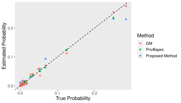
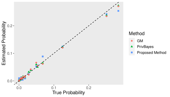
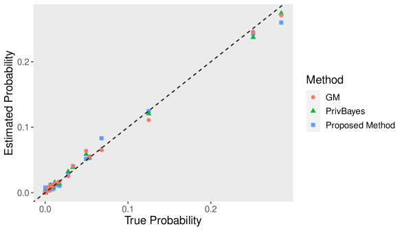
Figure 3: Plots of true full table probabilities versus estimated full table probabilities for $\epsilon\in\{0.25,0.5,1.0$}. Comparison of latent class modeling approach with a graphical models-based approach and PrivBayes for $\epsilon=0.25$ (top), $0.50$ (middle), and $1.00$ (bottom). For the proposed approach, estimated full cell probabilities denote the mean of the corresponding posterior distribution.

5 Application to the National Long-Term Care Survey

In this section we illustrate the latent class approach on a large-scale dataset from the National Long Term Care Survey (NLTCS).

5.1 Data Description

The NLTCS is a longitudinal survey sponsored by the U.S. National Institute on Aging. First developed in 1982, the survey selects participants from Medicare enrollment files. All participants are over the age of 65, and new participants are added to the survey every five years (National Institute on Aging, 2021). Access to the data is restricted but can be obtained through an approved protocol (Manton, 2010). For this analysis, we restricted ourselves to the 2004 wave of the NLTCS. In addition, we focused on sixteen variables representing markers of daily living as defined in Table 4. Participants with missing or unknown values for any of these variables were dropped, resulting in a $2^{16}$ contingency table comprised of $n=15,636$ observations.

Table 4: Data description for the NLTCS variables. Data was collected from the 2004 wave of the NLTCS. All variables had two levels: “yes” and “no”.

Variable	Description	Counts by Level
SCN_15_A_Y04	Problem eating by self	“yes”: 416; “no”: 15,220
SCN_15_B_Y04	Problem getting in/out of bed by self	“yes”: 862; “no”: 14,774
SCN_15_C_Y04	Problem getting in/out of chairs by self	“yes”: 1,054; “no”: 14,582
SCN_15_D_Y04	Problem walking inside without help	“yes”: 1,763; “no”: 13,873
SCN_15_E_Y04	Problem going outside without help	“yes”: 2,435; “no”: 13,201
SCN_15_F_Y04	Problem dressing without help	“yes”: 929; “no”: 14,707
SCN_15_G_Y04	Problem bathing without help	“yes”: 1,358; “no”: 14,278
SCN_15_H_Y04	Problem going to the bathroom without help	“yes”: 842; “no”: 14,794
SCN_15_I_Y04	Incontinence	“yes”: 1,355; “no”: 14,281
SCN_17_A_Y04	Prepare meals without help	“yes”: 13,670; “no”: 1,966
SCN_17_B_Y04	Do laundry without help	“yes”: 13,465; “no”: 2,171
SCN_17_C_Y04	Light housework without help	“yes”: 13,853; “no”: 1,783
SCN_17_D_Y04	Shop for groceries without help	“yes”: 12,678; “no”: 2,958
SCN_17_E_Y04	Manage money without help	“yes”: 13,737; “no”: 1,899
SCN_17_F_Y04	Take medicine without help	“yes”: 14,031; “no”: 1,605
SCN_17_G_Y04	Make phone calls without help	“yes”: 14,251; “no”: 1,385

5.2 Implementation Details

The 16 binary variables make ${16\choose 2}=120$ two-way marginal tables and $120\times(2\times 2)=480$ marginal counts. We selected important margins using the first half of the PrivBayes routine using a quarter of our privacy budget. While this allocates some of our privacy budget, it greatly reduces the number of marginals used in estimating model parameters. This resulted in 29 two-way margins. All counts were used for each pair, corresponding to $29\times(2\times 2)=116$ marginal counts.

As before, we used a Metropolis-within-Gibbs algorithm to sample from the posterior distribution of $\boldsymbol{\pi_{k}}$, $\boldsymbol{\psi_{k}}$ and $(M_{1},\ldots,M_{k})$. To avoid overparametrization of the model, we set the number of latent classes to seven, ensuring that the number of estimated parameters (118) is roughly equal to the number of input marginals (116). We follow a similar implementation strategy as our ACS example; see Supplementary Section 2 for details. We run the chain for 12,000 iterations with the first 2,000 discarded as burn-in. We use four values of $\epsilon$: $0.5$, $1.0$, $2.0$, and $5.0$. We estimate the two-way marginal probabilities at each iteration using $\boldsymbol{\pi_{k}}$ and $\boldsymbol{\psi_{k}}$.

5.3 Results

For each of the 116 marginal counts, we compare the estimated and original (non-noisy) two-way probabilities. Figure 4 displays the log ratio (or difference e.g., $\log(P_{est}/P_{true})$) by $\epsilon$. The plotted marginal counts are ranked in order according to the true count with the smallest counts being on the left. The average log difference across all counts ranged from 0.173 for $\epsilon=0.5$ to 0.050 for $\epsilon=5$. The estimates with $\epsilon=0.5$ are improved over using the noisy marginal counts directly: the noisy marginal counts had an average log difference of -0.297 for $\epsilon=0.5$. However, when $\epsilon=5$, the results from the noisy count are better, having an average log difference of 0.002.

Two observations are readily apparent from Figure 4. First, log differences appear to decrease as a function of $\epsilon$ with higher values corresponding to greater similarity between the estimated and true marginal probabilities. Second, log differences appear to be greater for smaller marginal probabilities regardless of $\epsilon$. This result is somewhat unsurprising when considering the structure of our model: the variance of the binomial distribution directly corresponds to the probability. In fact, at the sample size of our data, the variance at the minimum marginal probability is 46 times smaller than the corresponding variance at 25%. This effect is not as extreme at larger probabilities as the maximum marginal probability is approximately 92.5%.

Furthermore, the vast majority of the log differences at these lower counts are positive, indicating that the estimated marginal probability is greater than the true marginal probability. We believe that this result is amplified by the inherent non-negativity of the counts and sampling from the simplex.

The main benefit of the latent class modeling approach is the capability to facilitate posterior inferences and to generate synthetic data. For the former, we computed 95% credible intervals for each marginal probability by selecting the 2.5^th and 97.5^th quantiles of the posterior draws. For the latter, we randomly selected 20 iterates of the MCMC chain, and used each set of parameter draws to sample 15,636 synthetic records. This creates 15,636 synthetic records that can summed to estimate probabilities in the full table. We computed the marginal probabilities in each synthetic data set and combined the estimates using the approach in Reiter (2003), resulting in 95% confidence intervals. Tables 5 and 6 present results for three randomly selected marginal tables for the credible intervals and synthetic data inferences, respectively. The posterior intervals and synthetic data intervals, which are quite similar, typically capture the true non-noisy estimate of the marginal probabilities, especially for larger values of $\epsilon$.

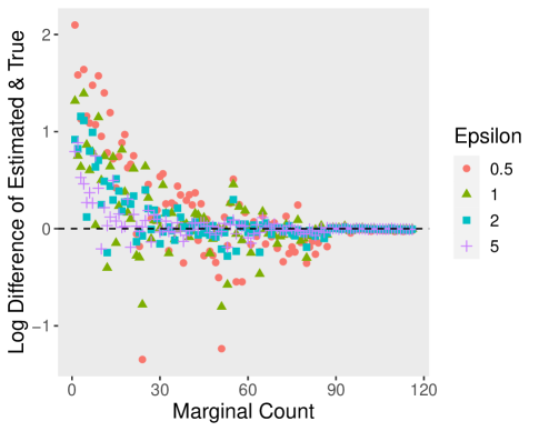
Figure 4: Plot of average log distance by marginal count for $\epsilon\in\{0.5,1.0,2.0,5.0$}. A log distance of zero indicates that the true and estimated probabilities are identical. Values greater than zero imply that the estimated probability is larger than the truth. Marginal counts are arranged in ascending order with the smallest counts on the left.

Table 5: Posterior intervals for selected marginal counts in the NLTCS example. Results also include the noisy counts input to the latent class model.

			$\epsilon$ = 0.5		$\epsilon$ = 1.0		$\epsilon$ = 2.0
		Pop.	Noisy		Noisy		Noisy
Variable	Cell	Est.	Est.	95% CI	Est.	95% CI	Est.	95% CI
	00	0.041	0.033	(0.053, 0.065)	0.041	(0.044, 0.052)	0.041	(0.040, 0.048)
SCN_15_E	01	0.114	0.112	(0.093, 0.107)	0.117	(0.106, 0.113)	0.114	(0.107, 0.116)
SCN_17_D	10	0.769	0.776	(0.762, 0.783)	0.770	(0.764, 0.774)	0.768	(0.768, 0.780)
	11	0.075	0.076	(0.062, 0.080)	0.075	(0.070, 0.077)	0.076	(0.065, 0.076)
	00	0.853	0.846	(0.839, 0.851)	0.849	(0.842, 0.849)	0.854	(0.853, 0.858)
SCN_17_B	01	0.008	0.007	(0.016, 0.033)	0.010	(0.013, 0.028)	0.008	(0.007, 0.011)
SCN_17_C	10	0.033	0.039	(0.032, 0.059)	0.033	(0.035, 0.043)	0.033	(0.030, 0.034)
	11	0.106	0.102	(0.067, 0.102)	0.107	(0.089, 0.102)	0.107	(0.102, 0.106)
	00	0.021	0.018	(0.013, 0.025)	0.021	(0.011, 0.019)	0.021	(0.015, 0.021)
SCN_15_C	01	0.046	0.046	(0.024, 0.044)	0.036	(0.034, 0.045)	0.046	(0.045, 0.050)
SCN_17_A	10	0.853	0.864	(0.846, 0.861)	0.854	(0.855,0.866)	0.852	(0.853, 0.859)
	11	0.080	0.084	(0.079, 0.105)	0.085	(0.079, 0.093)	0.080	(0.076, 0.081)

Table 6: Interval estimates based on 20 synthetic data sets for selected marginal counts in the NLTCS example. Point estimates, standard errors, and multipliers were computed using the combining rules of Reiter (2003).

			$\epsilon$ = 0.5	$\epsilon$ = 1.0	$\epsilon$ = 2.0
		Pop.	Point		Point		Point
Variable	Cell	Est.	Est.	95% CI	Est.	95% CI	Est.	95% CI
	00	0.041	0.057	(0.053, 0.061)	0.044	(0.041, 0.048)	0.044	(0.04, 0.047)
SCN_15_E	01	0.114	0.08	(0.076, 0.085)	0.091	(0.086, 0.096)	0.107	(0.102, 0.112)
SCN_17_D	10	0.769	0.806	(0.798, 0.815)	0.793	(0.786, 0.8)	0.779	(0.772, 0.786)
	11	0.075	0.056	(0.05, 0.061)	0.072	(0.067, 0.076)	0.07	(0.066, 0.074)
	00	0.853	0.879	(0.873, 0.886)	0.869	(0.864, 0.875)	0.86	(0.854, 0.865)
SCN_17_B	01	0.008	0.017	(0.014, 0.019)	0.012	(0.01, 0.015)	0.008	(0.007, 0.01)
SCN_17_C	10	0.033	0.034	(0.03, 0.039)	0.03	(0.027, 0.033)	0.03	(0.028, 0.033)
	11	0.106	0.07	(0.061, 0.078)	0.088	(0.083, 0.093)	0.102	(0.097, 0.106)
	00	0.021	0.016	(0.013, 0.018)	0.011	(0.008, 0.013)	0.017	(0.015, 0.019)
SCN_15_C	01	0.046	0.023	(0.018, 0.028)	0.032	(0.029, 0.036)	0.046	(0.042, 0.049)
SCN_17_A	10	0.853	0.886	(0.88, 0.892)	0.882	(0.876, 0.887)	0.86	(0.855, 0.866)
	11	0.080	0.076	(0.07, 0.081)	0.075	(0.071, 0.08)	0.077	(0.073, 0.081)

6 Concluding Remarks

We present a novel method for posterior inferences and creating differentially private synthetic data for contingency tables based on marginal counts. The simulation results indicate that the latent class modeling approach can offer reasonably accurate estimates of the counts used as inputs to construct the underlying tables (in our example, 2-way marginals). While it also did reasonably well in preserving counts from the full table in our illustrative data, analysts generally should not expect this to be the case. Rather than as a mechanism for generating data coherent with the full table probabilities, we view the approach as a means to make posterior inferences and generate synthetic data that are coherent with the marginal counts used as inputs. Thus, we advise agencies to tell data users what counts are used as inputs, so that data users do not expect the synthetic data to be accurate for other counts.

More generally, our approach is to define summary statistics as functions of model parameters, and use composite likelihood approximations to estimate those parameters. This general strategy can be extended to more complex data structures. For example, and as illustrated in the online supplement, the strategy could be used to generate synthetic data for people nested within households, using the latent class model of Hu et al. (2018) as the underlying model. Developing methods for practical implementation in such complex models is an area for future research.

We have shown in the NLTCS example that not all marginals are required to estimate our model. We leave it to future research to study methods for selecting the marginals, and, similarly, methods for allocating the privacy budget across these marginals. For both of our examples, we equally allocated the privacy budget. However, equal allocation may not be optimal in all problems.

References

- Abowd (2018) J. M. Abowd. The US Census Bureau adopts differential privacy. In Proceedings of the 24th ACM SIGKDD International Conference on Knowledge Discovery & Data Mining, pages 2867–2867. ACM, 2018. doi: 10.1145/3219819.3226070.
- Akande et al. (2019a) O. Akande, A. Barrientos, and J. P. Reiter. Simultaneous edit and imputation for household data with structural zeros. Journal of Survey Statistics and Methodology, 7(4):498–519, 2019a. doi: 10.1093/jssam/smy022.
- Akande et al. (2019b) O. Akande, J. Reiter, and A. F. Barrientos. Multiple imputation of missing values in household data with structural zeros. Survey Methodology, 2:498–519, 2019b. URL https://hdl.handle.net/10161/17537.
- Awan and Slavkovic (2021) J. Awan and A. Slavkovic. Structure and sensitivity in differential privacy: Comparing k-norm mechanisms. Journal of the American Statistical Association, 116(534):935–954, 2021. doi: 10.1080/01621459.2020.1773831. URL https://doi.org/10.1080/01621459.2020.1773831.
- Bao et al. (2021) E. Bao, X. Xiao, J. Zhao, D. Zhang, and B. Ding. Synthetic data generation with differential privacy via bayesian networks. Journal of Privacy and Confidentiality, 11(3), 2021.
- Barak et al. (2007) B. Barak, K. Chaudhuri, C. Dwork, S. Kale, F. McSherry, and K. Talwar. Privacy, accuracy, and consistency too: a holistic solution to contingency table release. In Proceedings of the twenty-sixth ACM SIGMOD-SIGACT-SIGART symposium on Principles of database systems, pages 273–282. ACM, 2007. doi: 10.1145/1265530.1265569.
- Barrientos et al. (2018) A. F. Barrientos, A. Bolton, T. Balmat, J. P. Reiter, J. M. de Figueiredo, A. Machanavajjhala, Y. Chen, C. Kneifel, M. DeLong, et al. Providing access to confidential research data through synthesis and verification: An application to data on employees of the US Federal Government. The Annals of Applied Statistics, 12(2):1124–1156, 2018. doi: 10.1214/18-AOAS1194.
- Benedetto et al. (2013) G. Benedetto, M. Stinson, and J. M. Abowd. The creation and use of the SIPP Synthetic Beta. Mimeo, U.S. Census Bureau, Apr. 2013. URL http://hdl.handle.net/1813/43924.
- Bowen and Liu (2016) C. M. Bowen and F. Liu. Comparative study of differentially private data synthesis methods. arXiv preprint arXiv:1602.01063, 2016.
- Bowen and Snoke (2019) C. M. Bowen and J. Snoke. Comparative study of differentially private synthetic data algorithms from the nist pscr differential privacy synthetic data challenge. arXiv preprint arXiv:1911.12704, 2019.
- Caiola and Reiter (2010) G. Caiola and J. P. Reiter. Random forests for generating partially synthetic, categorical data. Transaction on Data Privacy, 3:27–42, 2010. doi: 10.5555/1747335.1747337.
- Charest (2012) A.-S. Charest. Empirical evaluation of statistical inference from differentially-private contingency tables. In International Conference on Privacy in Statistical Databases, pages 257–272. Springer, 2012. doi: 10.1007/978-3-642-33627-0˙20.
- Chaudhuri et al. (2013) K. Chaudhuri, A. D. Sarwate, and K. Sinha. A near-optimal algorithm for differentially-private principal components. Journal of Machine Learning Research, 14, 2013.
- Drechsler (2009) J. Drechsler. Synthetic datasets for the German IAB Establishment Panel. Invited Paper WP.10, Joint UNECE/Eurostat work session on statistical data confidentiality, 2009. URL http://www.unece.org/fileadmin/DAM/stats/documents/ece/ces/ge.46/2009/wp.10.e.pdf.
- Drechsler (2011) J. Drechsler. Synthetic datasets for statistical disclosure control: Theory and implementation, volume 201 of Lecture Notes in Statistics. Springer Science & Business Media, 2011. ISBN 9781461403258. doi: 10.1007/978-1-4614-0326-5.
- Dunson and Xing (2009) D. B. Dunson and C. Xing. Nonparametric Bayes modeling of multivariate categorical data. Journal of the American Statistical Association, 104(487):1042–1051, 2009. doi: 10.1198/jasa.2009.tm08439.
- Dwork et al. (2006a) C. Dwork, K. Kenthapadi, F. McSherry, I. Mironov, and M. Naor. Our data, ourselves: Privacy via distributed noise generation. In Annual International Conference on the Theory and Applications of Cryptographic Techniques, pages 486–503. Springer, 2006a. doi: 10.1007/11761679˙29.
- Dwork et al. (2006b) C. Dwork, F. McSherry, K. Nissim, and A. Smith. Calibrating noise to sensitivity in private data analysis. In Theory of cryptography conference, pages 265–284. Springer, 2006b. doi: 10.1007/978-3-540-32732-5˙32.
- Dwork et al. (2014) C. Dwork, A. Roth, et al. The algorithmic foundations of differential privacy. Foundations and Trends in Theoretical Computer Science, 9(3–4):211–407, 2014. doi: 10.1561/0400000042.
- Eugenio and Liu (2018) E. C. Eugenio and F. Liu. Construction of microdata from a set of differentially private low-dimensional contingency tables through solving linear equations with tikhonov regularization. arXiv preprint arXiv:1812.05671, 2018.
- Ferguson (1973) T. S. Ferguson. A bayesian analysis of some nonparametric problems. The annals of statistics, pages 209–230, 1973. URL https://www.jstor.org/stable/2958008.
- Fienberg and Slavkovic (2005) S. E. Fienberg and A. B. Slavkovic. Preserving the confidentiality of categorical statistical data bases when releasing information for association rules. Data Mining and Knowledge Discovery, 11(2):155–180, 2005.
- Fuller (2009) W. A. Fuller. Measurement Error Models, volume 305. John Wiley & Sons, 2009. doi: 10.1002/9780470316665.
- Garfinkel et al. (2018) S. L. Garfinkel, J. M. Abowd, and S. Powazek. Issues encountered deploying differential privacy. In Proceedings of the 2018 Workshop on Privacy in the Electronic Society, pages 133–137. ACM, 2018. doi: 10.1145/3267323.3268949.
- Gelman et al. (2013) A. Gelman, J. B. Carlin, H. S. Stern, D. B. Dunson, A. Vehtari, and D. B. Rubin. Bayesian data analysis. CRC press, 2013.
- Ghosh et al. (2012) A. Ghosh, T. Roughgarden, and M. Sundararajan. Universally utility-maximizing privacy mechanisms. SIAM Journal on Computing, 41(6):1673–1693, 2012. doi: 10.1145/1536414.1536464.
- Gong (2019) R. Gong. Exact inference with approximate computation for differentially private data via perturbations. arXiv preprint arXiv:1909.12237, 2019.
- Hardt et al. (2012) M. Hardt, K. Ligett, and F. McSherry. A simple and practical algorithm for differentially private data release. In Advances in Neural Information Processing Systems, pages 2339–2347, 2012. doi: 10.5555/2999325.2999396.
- Hay et al. (2010) M. Hay, V. Rastogi, G. Miklau, and D. Suciu. Boosting the accuracy of differentially private histograms through consistency. Proceedings of the VLDB Endowment, 3(1-2):1021–1032, 2010. doi: 10.14778/1920841.1920970.
- Hu et al. (2018) J. Hu, J. P. Reiter, Q. Wang, et al. Dirichlet process mixture models for modeling and generating synthetic versions of nested categorical data. Bayesian Analysis, 13(1):183–200, 2018. doi: 10.1214/16-BA1047.
- Hundepool et al. (2012) A. Hundepool, J. Domingo-Ferrer, L. Franconi, S. Giessing, E. S. Nordholt, K. Spicer, and P.-P. De Wolf. Statistical disclosure control. John Wiley & Sons, 2012. doi: 10.1002/9781118348239.
- Inusah and Kozubowski (2006) S. Inusah and T. J. Kozubowski. A discrete analogue of the Laplace distribution. Journal of statistical planning and inference, 136(3):1090–1102, 2006. doi: 10.1016/j.jspi.2004.08.014.
- Ishwaran and James (2001) H. Ishwaran and L. F. James. Gibbs sampling methods for stick-breaking priors. Journal of the American Statistical Association, 96(453):161–173, 2001. doi: 10.1198/016214501750332758.
- Karr et al. (2006) A. F. Karr, C. N. Kohnen, A. Oganian, J. P. Reiter, and A. P. Sanil. A framework for evaluating the utility of data altered to protect confidentiality. The American Statistician, 60(3):224–232, 2006. doi: 10.1198/000313006X124640.
- Karwa et al. (2015) V. Karwa, D. Kifer, and A. B. Slavković. Private posterior distributions from variational approximations. arXiv preprint arXiv:1511.07896, 2015.
- Karwa et al. (2017) V. Karwa, P. N. Krivitsky, and A. B. Slavković. Sharing social network data: differentially private estimation of exponential family random-graph models. Journal of the Royal Statistical Society Series C, 66(3):481–500, 2017. doi: 10.1111/rssc.12185.
- Kinney et al. (2011) S. K. Kinney, J. P. Reiter, A. P. Reznek, J. Miranda, R. S. Jarmin, and J. M. Abowd. Towards unrestricted public use business microdata: The synthetic Longitudinal Business Database. International Statistical Review, 79(3):362–384, 2011. doi: 10.1111.j.1751-5823.2011.00153.x.
- Lee et al. (2015) J. Lee, Y. Wang, and D. Kifer. Maximum likelihood postprocessing for differential privacy under consistency constraints. In Proceedings of the 21th ACM SIGKDD International Conference on Knowledge Discovery and Data Mining, pages 635–644, 2015. doi: 10.1145/2783258.2783366.
- Li et al. (2018) B. Li, V. Karwa, A. Slavković, and R. C. Steorts. A privacy preserving algorithm to release sparse high-dimensional histograms. Journal of Privacy and Confidentiality, 8(1), 2018. doi: 10.29012/jpc.657.
- Lindsay (1988) B. G. Lindsay. Composite likelihood methods. Contemporary mathematics, 80(1):221–239, 1988. doi: 10.1090/conm/080/999014.
- Little (1993) R. J. Little. Statistical analysis of masked data. Journal of Official Statistics, 9(2):407–426, 1993.
- Machanavajjhala et al. (2008) A. Machanavajjhala, D. Kifer, J. M. Abowd, J. Gehrke, and L. Vilhuber. Privacy: Theory meets practice on the map. International Conference on Data Engineering (ICDE), pages 277–286, 2008. doi: 10.1109/ICDE.2008.4497436.
- Manrique-Vallier and Reiter (2014) D. Manrique-Vallier and J. P. Reiter. Bayesian estimation of discrete multivariate latent structure models with structural zeros. Journal of Computational and Graphical Statistics, 23(4):1061–1079, 2014. doi: 10.1080/10618600.2013.844700.
- Manton (2010) K. G. Manton. National long-term care survey: 1982, 1984, 1989, 1994, 1999, and 2004, 2010. URL https://doi.org/10.3886/ICPSR09681.v5.
- Mateo-Sanz et al. (2004) J. M. Mateo-Sanz, A. Martínez-Ballesté, and J. Domingo-Ferrer. Fast generation of accurate synthetic microdata. In International Workshop on Privacy in Statistical Databases, pages 298–306. Springer, 2004. doi: 10.1007/978-3-540-25955-8˙24.
- McKenna et al. (2019) R. McKenna, D. Sheldon, and G. Miklau. Graphical-model based estimation and inference for differential privacy. arXiv preprint arXiv:1901.09136, 2019.
- McKenna et al. (2021a) R. McKenna, G. Miklau, and D. Sheldon. Winning the NIST contest: A scalable and general approach to differentially private synthetic data. 11, 2021a. URL https://journalprivacyconfidentiality.org/index.php/jpc/article/view/778.
- McKenna et al. (2021b) R. McKenna, G. Miklau, and D. Sheldon. Winning the nist contest: A scalable and general approach to differentially private synthetic data. Journal of Privacy and Confidentiality, 11(3), 2021b.
- McSherry (2009) F. D. McSherry. Privacy integrated queries: an extensible platform for privacy-preserving data analysis. In Proceedings of the 2009 ACM SIGMOD International Conference on Management of data, pages 19–30. ACM, 2009. doi: 10.1145/1559845.1559850.
- Mironov (2017) I. Mironov. Rényi differential privacy. In 2017 IEEE 30th Computer Security Foundations Symposium (CSF), pages 263–275. IEEE, 2017. doi: 10.1109/CSF.2017.11.
- National Institute of Standards and Technology (2021) National Institute of Standards and Technology. 2018 differential privacy synthetic data challenge, 2021. URL https://www.nist.gov/ctl/pscr/open-innovation-prize-challenges/past-prize-challenges/2018-differential-privacy-synthetic.
- National Institute on Aging (2021) National Institute on Aging. National long term care survey (nltcs), 2021. URL https://www.nia.nih.gov/research/resource/national-long-term-care-survey-nltcs.
- Park and Ghosh (2014) Y. Park and J. Ghosh. Pegs: Perturbed gibbs samplers that generate privacy-compliant synthetic data. Transactions on Data Privacy, 7(3):253–282, 2014. doi: 10.5555/2870614.2870617.
- Ping et al. (2017) H. Ping, J. Stoyanovich, and B. Howe. Datasynthesizer: Privacy-preserving synthetic datasets. In Proceedings of the 29th International Conference on Scientific and Statistical Database Management, pages 1–5, 2017. doi: 10.1145/3085504.3091117.
- Raab (2019) G. Raab. Practical experience with making synthetic data differentially private, 2019. URL https://simons.berkeley.edu/talks/tba-47.
- Reiter (2003) J. P. Reiter. Inference for partially synthetic, public use microdata sets. Survey Methodology, 29:181–188, 2003.
- Reiter (2005a) J. P. Reiter. Estimating risks of identification disclosure in microdata. Journal of the American Statistical Association, 100(472):1103–1112, 2005a. doi: 10.1198/016214505000000619.
- Reiter (2005b) J. P. Reiter. Using CART to generate partially synthetic public use microdata. Journal of Official Statistics, 21(3):441–462, 2005b.
- Reiter et al. (2014) J. P. Reiter, Q. Wang, and B. Zhang. Bayesian estimation of disclosure risks for multiply imputed, synthetic data. Journal of Privacy and Confidentiality, 6(1), 2014. doi: 10.29012/jpc.v6i1.635.
- Rinott et al. (2018) Y. Rinott, C. M. O’Keefe, N. Shlomo, C. Skinner, et al. Confidentiality and differential privacy in the dissemination of frequency tables. Statistical Science, 33(3):358–385, 2018. URL https://projecteuclid.org/euclid.ss/1534147228.
- Roy (2020) V. Roy. Convergence diagnostics for markov chain monte carlo. Annual Review of Statistics and Its Application, 7:387–412, 2020.
- Rubin (1993) D. B. Rubin. Discussion: Statistical disclosure limitation. Journal of Official Statistics, 9(2):461–468, 1993.
- Seeman et al. (2020) J. Seeman, A. Slavkovic, and M. Reimherr. Private posterior inference consistent with public information: a case study in small area estimation from synthetic census data. In International Workshop on Privacy in Statistical Databases. Springer, 2020. doi: 10.1007/978-3-030-57521-2˙23.
- Si and Reiter (2013) Y. Si and J. P. Reiter. Nonparametric bayesian multiple imputation for incomplete categorical variables in large-scale assessment surveys. Journal of Educational and Behavioral Statistics, 38(5):499–521, 2013. doi: 10.3102/1076998613480394.
- Slavković et al. (2015) A. Slavković, X. Zhu, and S. Petrović. Fibers of multi-way contingency tables given conditionals: relation to marginals, cell bounds and markov bases. Annals of the Institute of Statistical Mathematics, 67(4):621–648, 2015. doi: 10.1007/s10463-014-0471-z. URL https://doi.org/10.1007/s10463-014-0471-z.
- Slavković and Lee (2010) A. B. Slavković and J. Lee. Synthetic two-way contingency tables that preserve conditional frequencies. Statistical Methodology, 7(3):225–239, 2010. doi: 10.1016/j.stamet.2009.11.002.
- SLS-DSU (2018) SLS-DSU. Scottish Longitudinal Study Development & Support Unit, 2018. URL https://sls.lscs.ac.uk/.
- Snoke and Slavković (2018) J. Snoke and A. Slavković. pMSE mechanism: Differentially private synthetic data with maximal distributional similarity. arXiv preprint arXiv:1805.09392, 2018.
- Snoke et al. (2018) J. Snoke, G. M. Raab, B. Nowok, C. Dibben, and A. Slavkovic. General and specific utility measures for synthetic data. Journal of the Royal Statistical Society: Series A (Statistics in Society), 181(3):663–688, 2018. doi: 10.1111/rssa.12358.
- Ullman and Vadhan (2020) J. Ullman and S. Vadhan. Pcps and the hardness of generating synthetic data. Journal of Cryptology, 33(4):2078–2112, 2020.
- Varin et al. (2011) C. Varin, N. Reid, and D. Firth. An overview of composite likelihood methods. Statistica Sinica, pages 5–42, 2011. URL https://www.jstor.org/stable/24309261.
- Walker (2013) S. G. Walker. Bayesian inference with misspecified models. Journal of Statistical Planning and Inference, 143(10):1621–1633, 2013. doi: 10.1016/j.jspi.2013.05.013.
- Woo and Slavković (2012) Y. M. J. Woo and A. B. Slavković. Logistic regression with variables subject to post randomization method. In International Conference on Privacy in Statistical Databases, pages 116–130. Springer, 2012. doi: 10.1007/978-3-642-33627-0˙10.
- Woodcock and Benedetto (2009) S. D. Woodcock and G. Benedetto. Distribution-preserving statistical disclosure limitation. Computational Statistics & Data Analysis, 53(12):4228–4242, 2009. doi: 10.1016/j.csda.2009.05.020.
- Yang et al. (2012) X. Yang, S. E. Fienberg, and A. Rinaldo. Differential privacy for protecting multi-dimensional contingency table data: Extensions and applications. Journal of Privacy and Confidentiality, 4(1), 2012. doi: 10.29012/jpc.v4i1.613.
- Zhang et al. (2012) J. Zhang, Z. Zhang, X. Xiao, Y. Yang, and M. Winslett. Functional mechanism: regression analysis under differential privacy. Proceedings of the VLDB Endowment, 5(11):1364–1375, 2012. doi: 10.14778/2350229.2350253.
- Zhang et al. (2017) J. Zhang, G. Cormode, C. M. Procopiuc, D. Srivastava, and X. Xiao. PrivBayes: Private data release via Bayesian networks. ACM Transactions on Database Systems, 42(4):1–41, 2017. doi: 10.1145/3134428.