: Multi-Scale Representation Learning over a Spherical Surface for Geospatial Predictions

Abstract

Generating learning-friendly representations for points in a 2D space is a fundamental and long-standing problem in machine learning. Recently, multi-scale encoding schemes (such as Space2Vec) were proposed to directly encode any point in 2D space as a high-dimensional vector, and has been successfully applied to various (geo)spatial prediction tasks. However, a map projection distortion problem rises when applying location encoding models to large-scale real-world GPS coordinate datasets (e.g., species images taken all over the world) - all current location encoding models are designed for encoding points in a 2D (Euclidean) space but not on a spherical surface, e.g., earth surface. To solve this problem, we propose a multi-scale location encoding model called $\modelname$ which directly encodes point coordinates on a spherical surface while avoiding the map projection distortion problem. We provide theoretical proof that the $\modelname$ encoding preserves the spherical surface distance between any two points. We also developed a unified view of distance-reserving encoding on spheres based on the Double Fourier Sphere (DFS). We apply $\modelname$  to the geo-aware image classification task. Our analysis shows that $\modelname$  outperforms other 2D space location encoder models especially on the polar regions and data-sparse areas for image classification tasks because of its nature for spherical surface distance preservation.

1 Introduction

Location encoders [9, 21, 25, 41] refer to neural network architectures which encode a point in a 2D space (or 3D Euclidean space [41]) into a high dimensional embedding such that this kind of distributed representations are more learning-friendly for downstream machine learning models. Location encoders can be incorporated into the state-of-art models for many tasks to make them spatially explicit [40, 19]. In fact, location encoders have already shown promising performances on multiple tasks across different domains including geo-aware image classification [9, 21, 25], POI classification [25], trajectory prediction [39], geographic question answering [23], and 3D protein structure reconstruction [41]. Compared with well-established kernal-based approaches [31, 39] such as Radius Based Function (RBF) which requires to memorize the training examples as the kernel centers for a robust prediction, inductive-learning-based location encoders [9, 21, 25, 41] have many advantages: 1) they are more memory efficient since they do not need to memorize training samples; 2) unlike RBF, the performance on unseen locations does not depend on the number and distribution of kernels. Moreover, Gao et al. [14] have shown that grid like periodic representation can preserve absolute position information, relative distance and direction information in 2D Euclidean space. [25] further show that it benefit the generalizability of down-steam models.

(a) $\modelname$ Illustration

(b) Vulpes lagopus

(c) $wrap*$

(d) $grid$

(e) $sphereC+$

Figure 1: (a)Applying $\modelname$ model for geo-aware image classification; (b): iNat2018 training image locations for Vulpes lagopus (Arctic fox). (c)-(e): The predicted distributions of Vulpes lagopus from different models - $wrap*$ [21], $grid$[25], and $sphereC+$ (our model). $sphereC+$ produces a more compact and fine-grain distribution on the polar region while $wrap*$ [21] turns to produce a over-generalized species distribution while $grid$[25] is between two of them. For more examples, please see Figure 4.

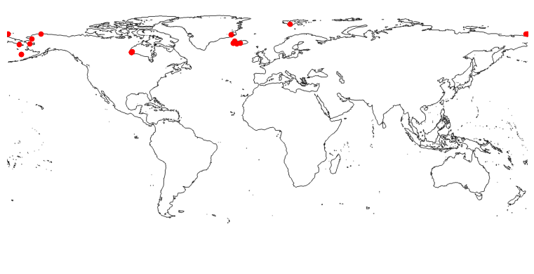
Demand on representation and prediction learning at a global scale grows dramatically due to emerging global scale issues, such as the transition path of the latest pandemic [7], long lasting issue for malaria [5], under threaten global biodiversity[13, 6], and numerous ecosystem and social system responses for climate change [16]. However, when applying the state-of-the-art 2D space location encoders [14, 9, 21, 25, 41] to large-scale real-world GPS coordinate datasets such as species images taken all over the world, a map projection distortion problem [37] emerges. These 2D location encoders are designed for preserving distance in 2D (or 3D) Euclidean space, while GPS coordinates are in fact spherical coordinates, e.g., point $\boldsymbol{\mathbf{x}}=(\lambda,\phi)$ on a sphere with longitude $\lambda\in[-\pi,\pi)$ and latitude $\phi\in[-{\pi}/{2},-{\pi}/{2}]$ (See Figure 1(a)). Directly applying these 2D location encoders on spherical coordinates will yield a large distortion in the polar regions. It is important to point out that map projection distortion is unavoidable when projecting spherical coordinates into 2D space. (See Appendix 9.1) This emphasizes the importance of calculating on a round planet [8].

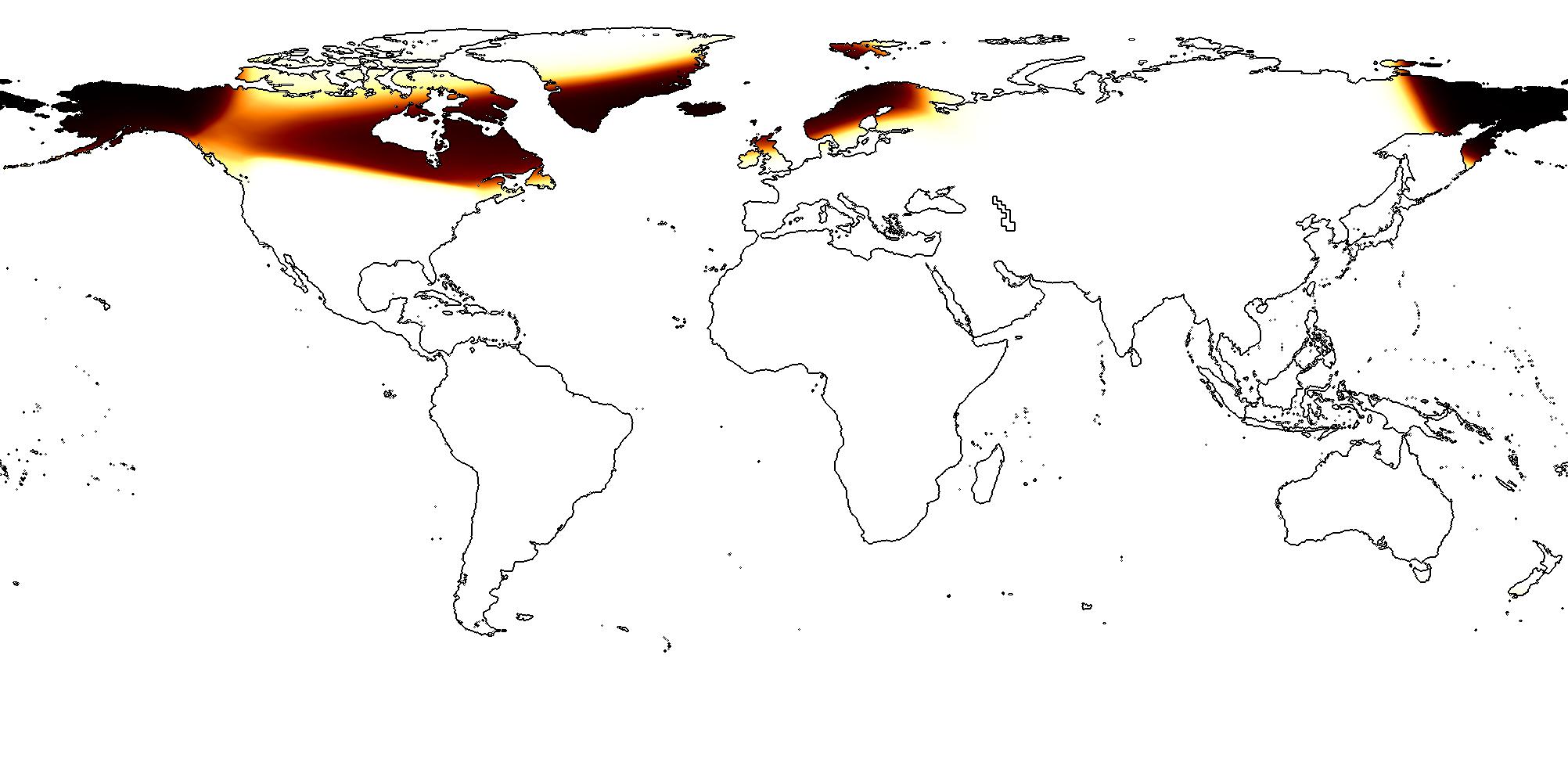
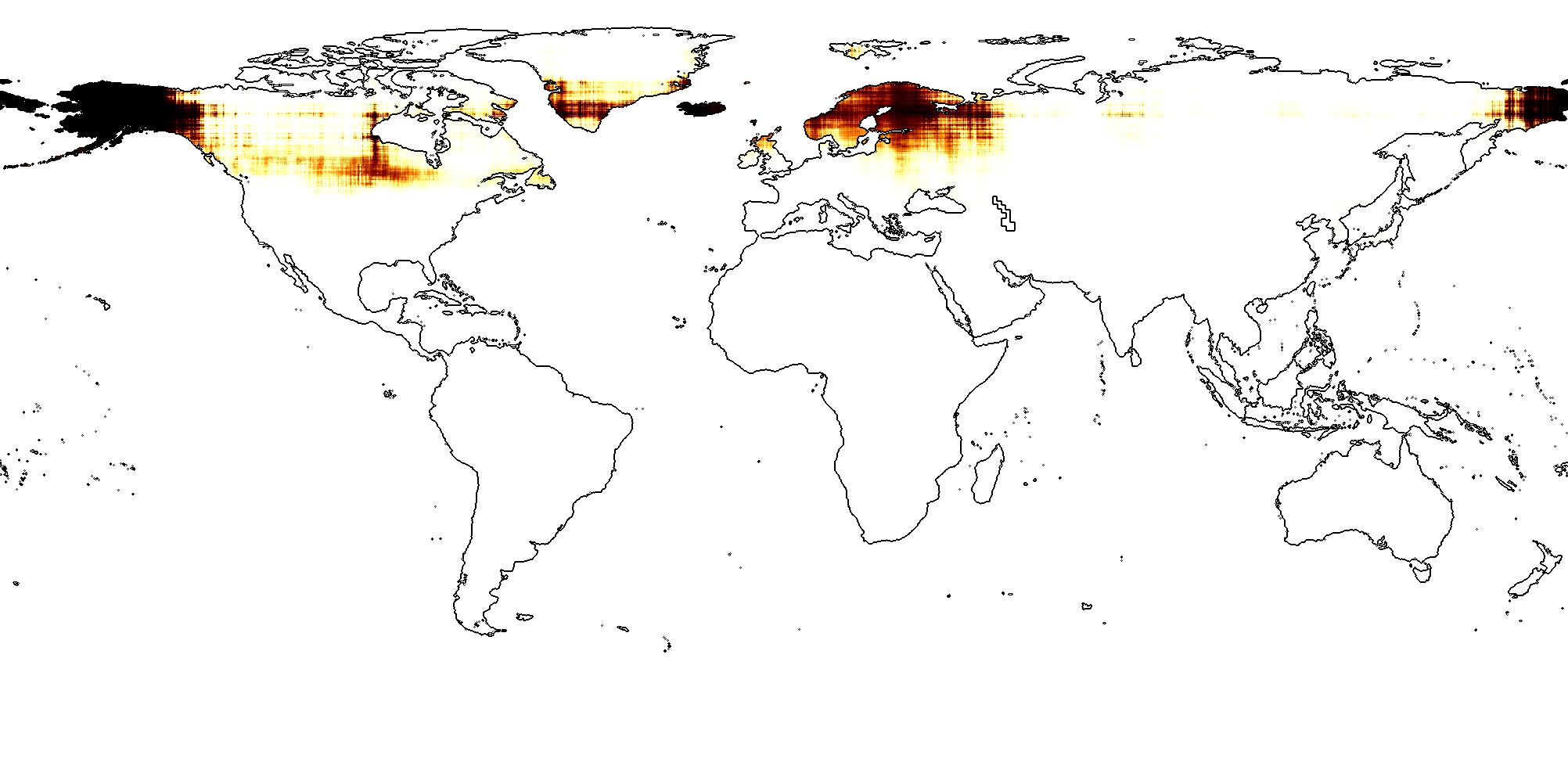
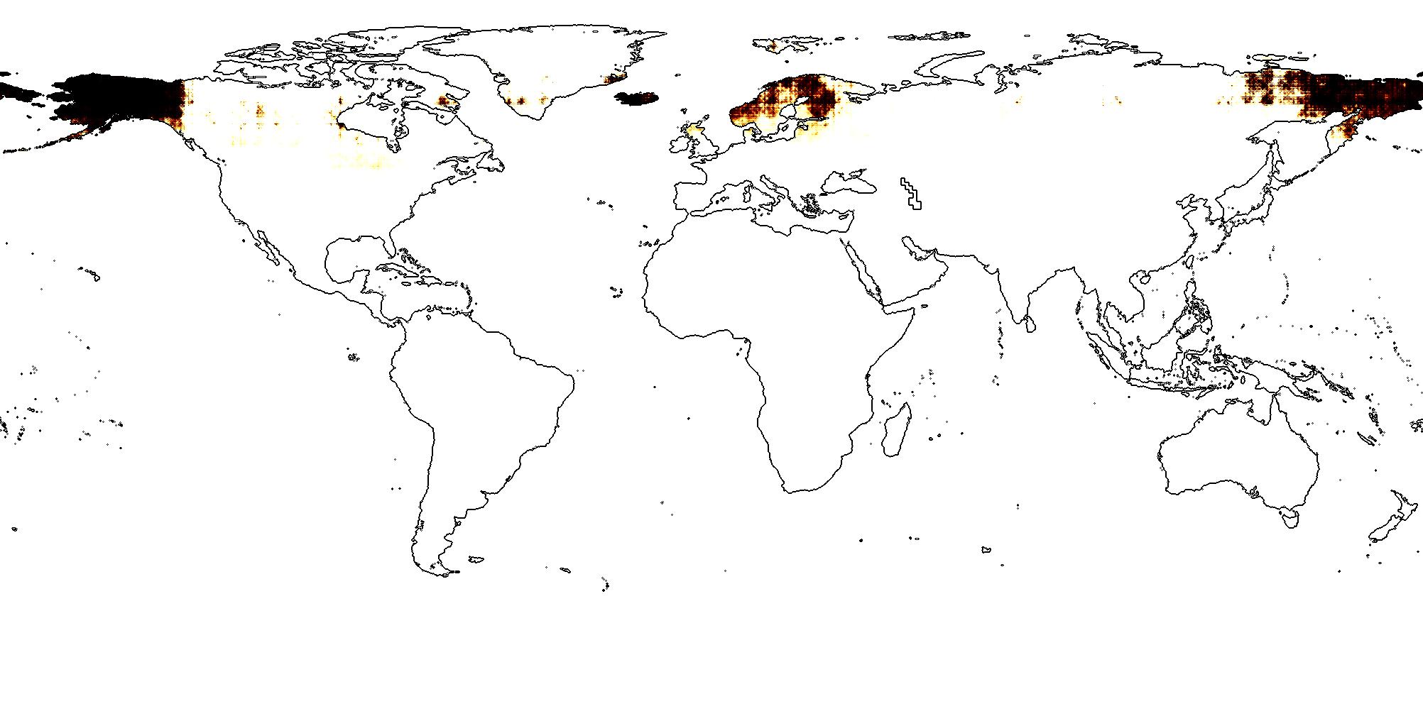
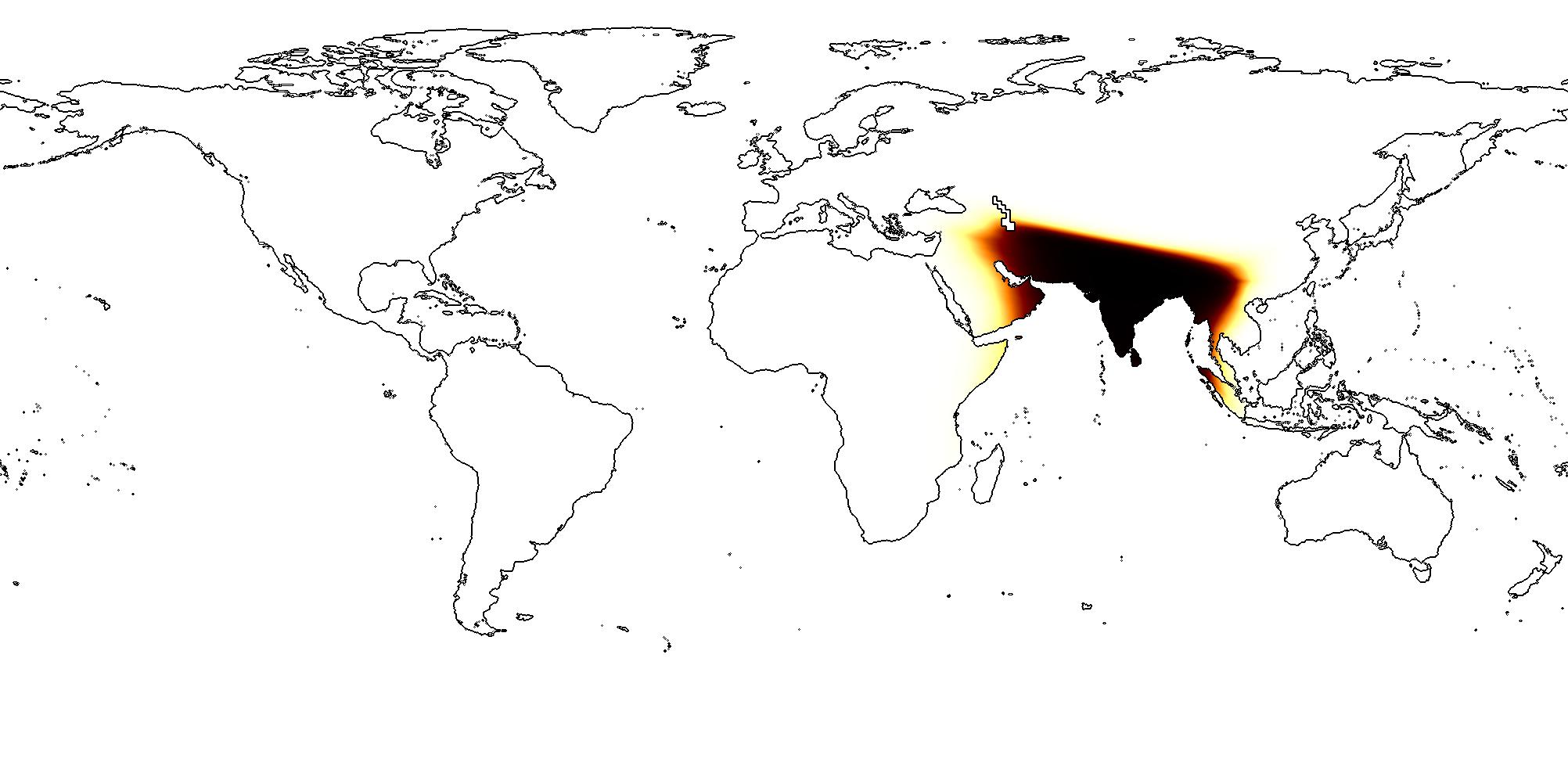
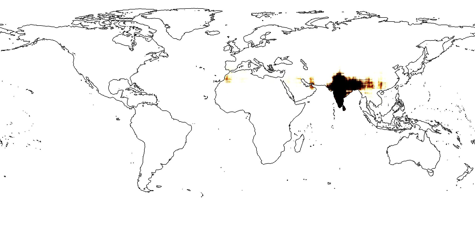
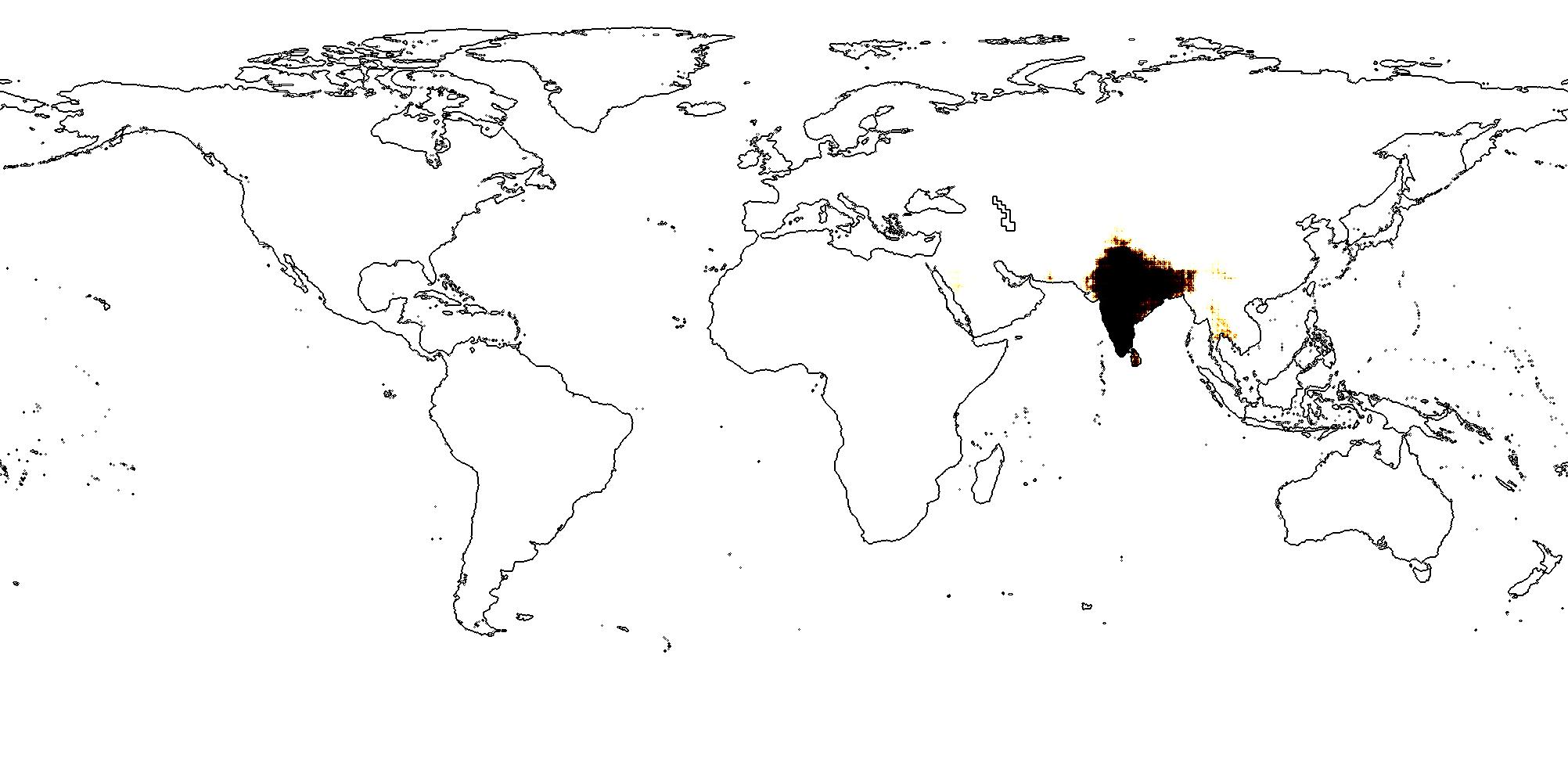
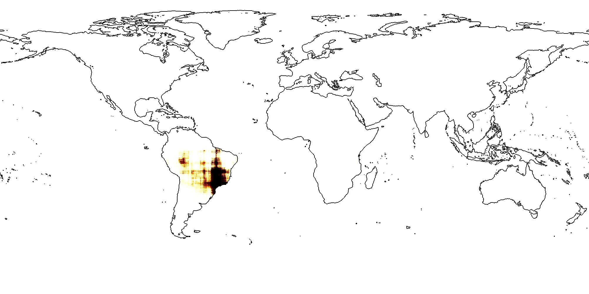
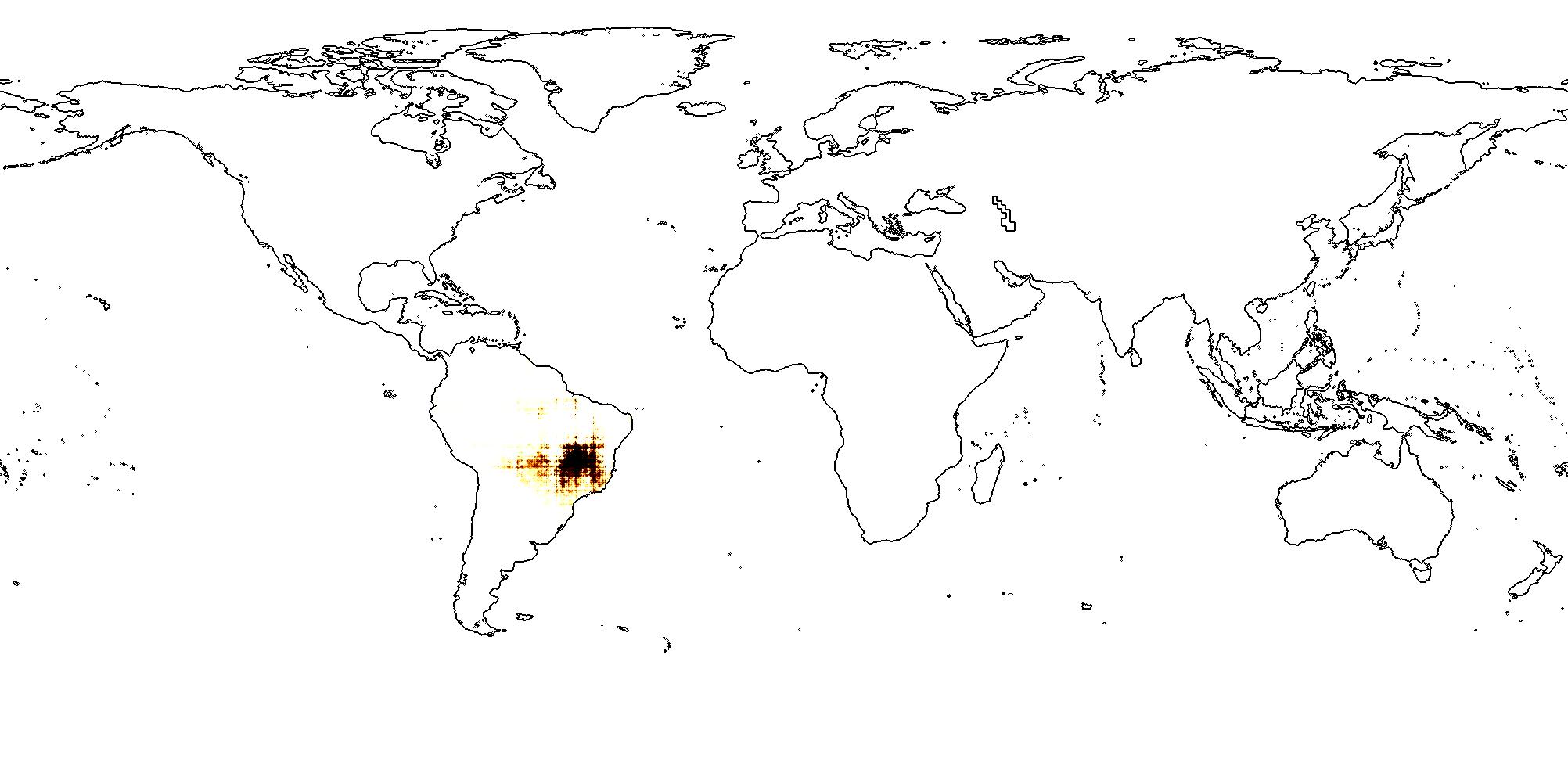
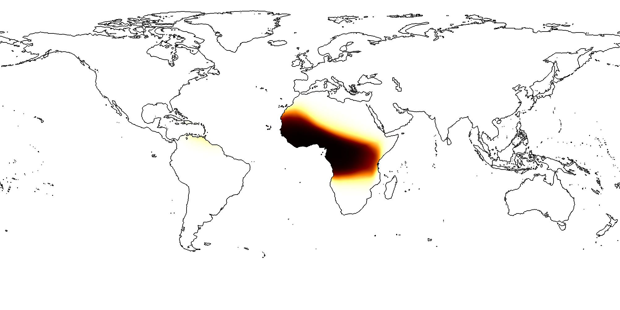
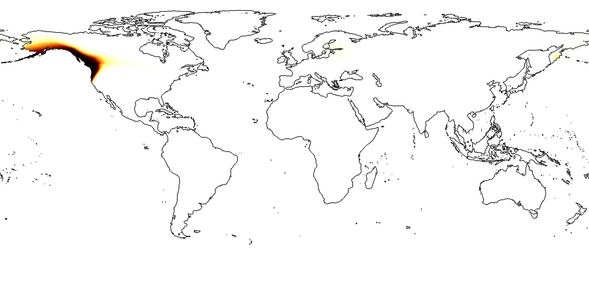
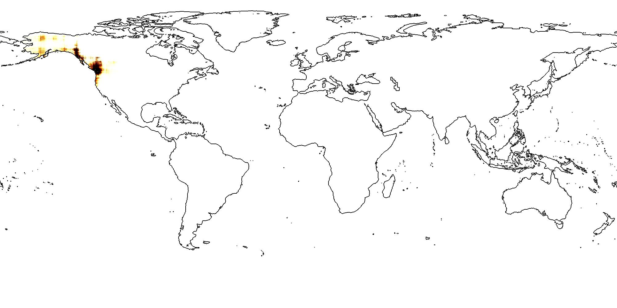
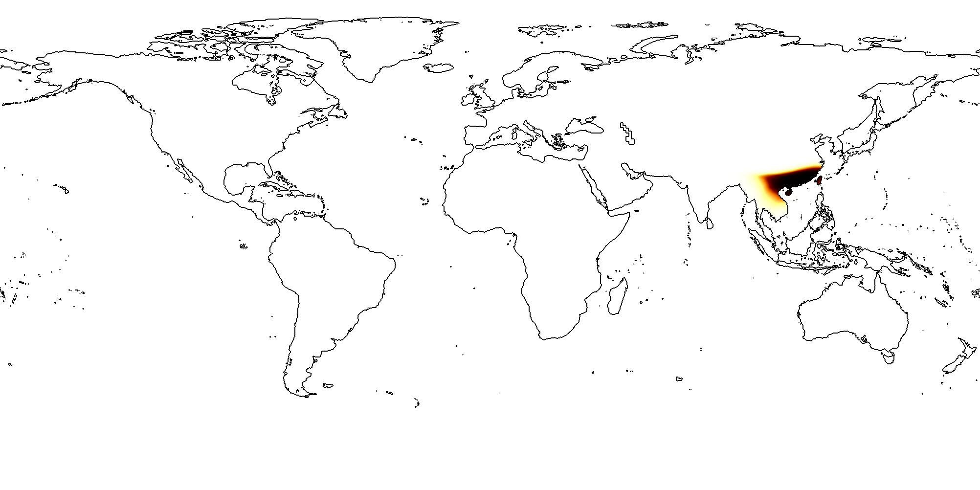
Due to the limitations of these 2D location encoders, there is an urgent need for a location encoding method which preserves the spherical distance (e.g., great circle distance) between two points. In this work, we propose $\modelname$, which can directly encode point coordinates on a spherical surface while avoiding the map projection distortion. The mutli-scale encoding method utilizes 2D Discrete Fourier Transform basis ($O(S^{2})$ terms) or a subset ($O(S)$ terms) of it while still being able to correctly measure the spherical distance. We demonstrate the effectiveness of $\modelname$ on the geo-aware image classification (or so-call species fine-grain recognition) [9, 21, 25]. Following previous work we use location encoding to learn the geographic prior distribution of different species so that given an image and its associated location, we can combine the prediction of the location encoder and that from the state-of-the-art image classification models, e.g., inception V3 [33], to improve the image classification accuracy. Figure 1(a) illsutrates the whole architecture. Given an image $\mathbf{I}$ in Figure 1(a), its very difficult to decide whether it is an arctic fox or gray fox just based on the appearance information. However, if we know this image is taken from the Arctic area, then we have more confidence to say this is a baby arctic fox (Vulpes lagopus). Figure 1 (c)-(e) shows the predicted distributions of Vulpes Lagopus from three different models. We can see that $\modelname$  has a clear advantage to capture fine-grained species distribution, especially on polar regions. In summary, the contributions of our work are:

1. We propose a multi-scale location encoder, $\modelname$, which, as far as we know, is the first inductive embedding encoding scheme which aims at preserving spherical distance.

2. We provide a theoretical proof that $\modelname$ encodings can preserve spherical surface distance between points. We also developed a unified view of distant reserving encoding methods on spheres based on Double Fourier Sphere (DFS) [26, 30].

3. We conduct extensive experiments on the geo-aware image classification task. Results show that due to its distance preserving ability, $\modelname$ outperforms the state-of-the-art 2D location encoder models. $\modelname$  is able to produce finer-grained and compact spatial distributions, and does significantly better on the polar regions and areas with sparse training samples.

2 Problem Formulation

Distributed representation of point-features on the spherical surface can be formulated as follows. Given a set of points $\mathcal{P}=\{\boldsymbol{\mathbf{x}}_{i}\}$ on the surface of a sphere $\mathbb{S}^{2}$, e.g., species occurrences all over the world, where $\boldsymbol{\mathbf{x}}_{i}=(\lambda_{i},\phi_{i})\in\mathbb{S}^{2}$ indicates a point with longitude $\lambda_{i}\in[-\pi,\pi)$ and latitude $\phi_{i}\in[-{\pi}/{2},{\pi}/{2}]$. Define a function $Enc_{\mathcal{P},\theta}(\boldsymbol{\mathbf{x}}):\mathbb{S}^{2}\to\mathbb{R}^{d}$, which is parameterized by $\theta$ and maps any coordinate $\boldsymbol{\mathbf{x}}$ in a spherical surface $\mathbb{S}^{2}$ to a vector representation of $d$ dimension.

Let $Enc(\boldsymbol{\mathbf{x}})=\mathbf{NN}(PE_{S}(\boldsymbol{\mathbf{x}}))$ where $\mathbf{NN}()$ is a learnable multi-layer perceptron with $h$ hidden layers and $k$ neurons per layer. We want to find a function $PE_{S}(\boldsymbol{\mathbf{x}})$ which does a one-to-one mapping from each point $\boldsymbol{\mathbf{x}}_{i}=(\lambda_{i},\phi_{i})\in\mathbb{S}^{2}$ to a multi-scale representation with $S$ as the total number of scales such that it satisfy the following requirement:

$$\langle PE_{S}(\boldsymbol{\mathbf{x}}_{1}),PE_{S}(\boldsymbol{\mathbf{x}}_{2})\rangle=f(\Delta D),\forall\boldsymbol{\mathbf{x}}_{1},\boldsymbol{\mathbf{x}}_{2}\in\mathbb{S}^{2},$$ (1)

where $\Delta D\in[0,\pi R]$ is the spherical surface distance between $\boldsymbol{\mathbf{x}}_{1},\boldsymbol{\mathbf{x}}_{2}$, $R$ is the radius of this sphere, and $f(x)$ is a strictly monotonically decreasing function for $x\in[0,\pi R]$. In other words, we expect to find a function $PE_{S}(\boldsymbol{\mathbf{x}})$ such that the resulting multi-scale representation of $\boldsymbol{\mathbf{x}}$ preserves the spherical surface distance while it is more learning-friendly for the downstream neuron network model $\mathbf{NN}()$.

3 Related Work

Location Encoder

There has been much research on developing inductive learning-based location encoders. Most of them directly apply Multi-Layer Perceptron (MLP) to 2D coordinates to get a high dimensional location embedding for downstream tasks such as pedestrian trajectory prediction [39] and geo-aware image classification [9]. Recently, Mac Adoha et al. [21] apply sinusoid functions to encode the latitude and longitude of each image before feeding into MLPs. All of the above approaches deploy encode locations at a single-scale.

Inspired by the position encoder in Transformer [35] and Neuroscience research on grid cells [1, 12] of mammals, Mai et al. [25] proposed to apply multi-scale sinusoid functions to encode locations in 2D space before feeding into MLPs. The multi-scale representations have advantages of capturing spatial feature distributions with different characteristics. Similarly, Zhong et al. [41] utilized a multi-scale location encoder for the position of proteins’ atoms in 3D Euclidean space for protein structure reconstruction with great success. For a comprehensive survey of different location encoders, please refer to Mai et al. [24].

Machine Learning Models on Spheres

There has been much recent work on solving map projection distortion when designing machine learning models for large-scale real-world datasets. For omnidirectional image classification task, both Cohen et al [10] and Coors et al. [11] design different spherical versions of the traditional CNN models in which the CNN filters explicitly considers map projection distortion. In terms of image geolocalization [17] and text geolocalization [18], a loss function based on the mixture of von Mises-Fisher distributions (MvMF)– a spherical analogue of the Gaussian mixture model (GMM)– is used to replace the traditional cross-entropy loss for geolocalization models [17, 18]. All these works are closely related to geometric deep learning [4]. They show the importance to consider the spherical geometry, yet none of them considers representation learning in the embedding space.

Spatially-Explicit Machine Learning Models

There has been much work in improving the performance of machine learning models by using spatial features or spatial inductive bias – so called spatially-explicit machine learning [19, 22], or SpEx-ML. The spatial inductive bias in these models includes: spatial dependency [20, 40], spatial heterogeneity [3, 9, 21, 25], map projection [10, 11, 17, 18], scale effect [36, 25], and so on.

Pseudospectral Methods on Spheres

Much study has been done for the numerical solutions on spheres, for example, in weather prediction [29, 30, 26]. The main idea is so called pseudospectral methods which leverage truncated discrete Fourier transformation on spheres to achieve computation efficiency while avoiding the error caused by projection distortion. The particular set of basis functions to be used depends on the particular problem. However, they do not aim at learning good representations in machine learning models. In this study we try to make connections to these approaches and explore how their insights can be realized in a deep learning model.

4 Method

In the following, we use $Enc(\boldsymbol{\mathbf{x}})$ to refer to $Enc_{\mathcal{P},\theta}(\boldsymbol{\mathbf{x}})$. In Section 4.1, we will discuss our main contribution - the design of spherical distance-kept location encoder $Enc(\boldsymbol{\mathbf{x}})$, $\modelname$. We developed a unified view of distance-reserving encoding on spheres based on Double Fourier Sphere (DFS) [26, 30]. Note that the resulting location embedding $\mathbf{p}[\boldsymbol{\mathbf{x}}]=Enc(\boldsymbol{\mathbf{x}})$ is a general-purpose embedding which can be utilized in different decoder architectures for various tasks. In Section 4.2, we briefly show how to utilize the proposed $Enc(\boldsymbol{\mathbf{x}})$ in the geo-aware image classification task.

4.1

Given any point $\boldsymbol{\mathbf{x}}=(\lambda,\phi)\in\mathbb{S}^{2}$ with longitude $\lambda\in[-\pi,\pi)$ and latitude $\phi\in[-\dfrac{\pi}{2},\dfrac{\pi}{2}]$, the multi-scale location encoder proposed is in the form of $Enc(\boldsymbol{\mathbf{x}})=\mathbf{NN}(PE_{S}(\boldsymbol{\mathbf{x}}))$. $PE_{S}(\boldsymbol{\mathbf{x}})$ is a concatenation of multi-scale spherical spatial features of $S$ levels. In the following, we call $Enc(\boldsymbol{\mathbf{x}})$ location encoder and its component $PE_{S}(\boldsymbol{\mathbf{x}})$ position encoder. Let $r_{min},r_{max}$ be the minimum and maximum scaling factor, and $g=\frac{r_{max}}{r_{min}}$.

(a) $sphereDFS$

(b) $grid$

(c) $sphereC$

(d) $sphereC+$

(e) $sphereM$

(f) $sphereM+$

Figure 2: Patterns of different encoders, blue points at $(\lambda^{m},\phi^{n})$ mean interaction terms of trigonometric functions of $\lambda^{m}$ and $\phi^{n}$ are included in the encoder, $\lambda$ and $\phi$ axis correspond to single terms with no interactions.

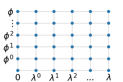
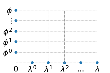
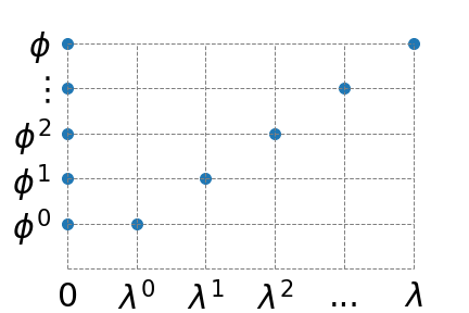
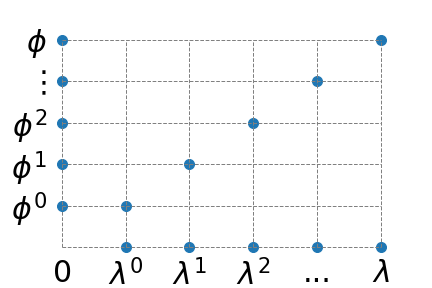
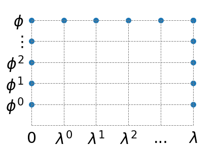
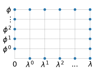
sphereDFS

Double Fourier Sphere (DFS) [26, 30] is a simple yet successful pseudospectral method, which is computationally efficient and have been applied to analysis of large scale phenomenons such as weather [32] and blackholes [2]. Our first intuition is to use the base functions of DFS to help decompose $\boldsymbol{\mathbf{x}}=(\lambda,\phi)$ into a high dimensional vector:

$$\begin{split}PE_{S,sphereDFS}(\boldsymbol{\mathbf{x}})=&\bigcup_{n=0}^{S-1}[\sin\phi_{n},\cos\phi_{n}]\cup\bigcup_{m=0}^{S-1}[\sin\lambda_{m},\cos\lambda_{m}]\cup\\ &\bigcup_{n=0}^{S-1}\bigcup_{m=0}^{S-1}[\cos\phi_{n}\cos\lambda_{m},\cos\phi_{n}\sin\lambda_{m},\sin\phi_{n}\cos\lambda_{m},\sin\phi_{n}\sin\lambda_{m}].\end{split}$$ (2)

where $\lambda_{s}=\frac{\lambda}{f^{s}}$, $\phi_{s}=\frac{\phi}{f^{s}}$, $f^{s}=r_{min}\cdot g^{s/(S-1)}$, $\cup$ means vector concatenation and $\bigcup_{s=0}^{S-1}$ indicates vector concatenation through different scales. It basically lets all the scales of $\phi$ terms interact with all the scales of $\lambda$ terms in the encoder. This would introduce an encoder whose output has $O(S^{2})$ dimensions and increase the memory burden in training and hurts generalization (Figure 2a). An encoder might achieve better result by only using a subset of these terms. In comparison, the state of art encoder such as $grid$ [25] and $wrap$ [21] define:

$$PE_{S,grid}(\boldsymbol{\mathbf{x}})=\bigcup_{s=0}^{S-1}[\sin\phi_{s},\cos\phi_{s},\sin\lambda_{s},\cos\lambda_{s}].$$ (3)

We can see that $grid$ employs a subset of terms from $sphereDFS$ (Figure 2b). As we explained earlier, $grid$ performs poorly at a global scale due to its inability to preserve spherical distances. In the following we explore different subsets of DFS terms while achieving two goals: 1) efficient representation with $O(S)$ dimensions 2) preserving distance measures on spheres.

sphereC

Inspired by the fact that any point $(x,y,z)$ in 3D Cartesian coordinate can be expressed by $sin$ and $cos$ basis of spherical coordinates ($\lambda$, $\phi$ plus radius) , we define the basic form of , namely $sphereC$ encoder, for scale $s$ as

$$PE_{S,sphereC}(\boldsymbol{\mathbf{x}})=\bigcup_{s=0}^{S-1}[\sin\phi_{s},\cos\phi_{s}\cos\lambda_{s},\cos\phi_{s}\sin\lambda_{s}].$$ (4)

To illustrate that $sphereC$ is good at capturing spherical distance, we take a close look at its basic case $S=1$ (define $s=0$ and $f^{s}=1$), where the multi-scale encoder degenerates to

$$PE_{1,sphereC}(\boldsymbol{\mathbf{x}})=[\sin(\phi),\cos(\phi)\cos(\lambda),\cos(\phi)\sin(\lambda)].$$ (5)

These three terms are included in the multi-scale version ($S>1$) and serve as the main terms at the largest scale and also the lowest frequency (when $s=S-1$). The high frequency terms are added to help the downstream neuron network to learn the point-feature more efficiently. Interestingly, $PE_{1,sphereC}$ captures the spherical distance in a very explicit way:

Theorem 1.

Let $\boldsymbol{\mathbf{x}}_{1}$, $\boldsymbol{\mathbf{x}}_{2}$ be two points on the same sphere with radius $R$, then

$$\langle PE_{1,sphereC}(\boldsymbol{\mathbf{x}}_{1}),PE_{1,sphereC}(\boldsymbol{\mathbf{x}}_{2})\rangle=\cos(\frac{\Delta D}{R}),$$ (6)

where $\Delta D$ is the great circle distance between $\boldsymbol{\mathbf{x}}_{1}$ and $\boldsymbol{\mathbf{x}}_{2}$. Under this metric,

$$\|PE_{1,sphereC}(\boldsymbol{\mathbf{x}}_{1})-PE_{1,sphereC}(\boldsymbol{\mathbf{x}}_{2})\|=2\sin(\frac{\Delta D}{2R}).$$ (7)

Moreover, $\|PE_{1,sphereC}(\boldsymbol{\mathbf{x}}_{1})-PE_{1,sphereC}(\boldsymbol{\mathbf{x}}_{2})\|\approx\frac{\Delta D}{R}$,when $\Delta D$ is small w.r.t. $R$.

See the proof in Section 5.1. Since the central angle $\Delta\delta=\frac{\Delta D}{R}\in[0,\pi]$ and $\cos(x)$ is strictly monotonically decrease for $x\in[0,\pi],$ Theorem 1 shows that $PE_{1,sphereC}(\boldsymbol{\mathbf{x}})$ directly satisfies our expectation in Equation 1 where $f(x)=\cos(\frac{x}{R})$. In comparison, the inner product in the output space of $grid$ encoder is

$$\langle PE_{1,grid}(\boldsymbol{\mathbf{x}}_{1}),PE_{1,grid}(\boldsymbol{\mathbf{x}}_{2})\rangle=\cos(\phi_{1}-\phi_{2})+\cos(\lambda_{1}-\lambda_{2}),$$ (8)

which models the latitude difference and longitude difference of $\boldsymbol{\mathbf{x}}_{1}$ and $\boldsymbol{\mathbf{x}}_{2}$ separately rather than spherical distance. This introduces problems in encoding. For instance, consider data pairs $\boldsymbol{\mathbf{x}}_{1}=(\lambda_{1},\phi)$ and $\boldsymbol{\mathbf{x}}_{2}=(\lambda_{2},\phi)$, the distance between them in output space of $grid$, $\|PE_{1,grid}(\boldsymbol{\mathbf{x}}_{1})-PE_{1,grid}(\boldsymbol{\mathbf{x}}_{2})\|^{2}=2-2\cos(\lambda_{1}-\lambda_{2})$ stays as a constant in terms of $\phi$. However, when $\phi$ varies from $-\frac{\pi}{2}$ to $\frac{\pi}{2}$, the actual spherical distance changes in a wide range, e.g., the actual distance between the data pair at $\phi=-\frac{\pi}{2}$ (South Pole) is 0 while the distance between the data pair at $\phi=0$ (Equator), gets the maximum value. This issue in measuring distances also has a negative impact on $grid$’s ability to model distributions in areas with sparse sample points because it is hard to learn the true spherical distance. We observe that $grid$ reaches peak performance at much smaller $r_{min}$ than that of $\modelname$ encodings (See Appendix 9.3). Moreover, $sphereC$ outperforms $grid$ near polar regions where $grid$ claims large distance though the spherical distance is small (A, B in Figure 1(a)).

sphereM

Considering the fact that many geographical features are more sensitive to either latitude (e.g., temperature, sunshine duration) or longitude (e.g., timezones, geopolitical borderlines), we might want to focus on increasing the resolution of either $\phi$ or $\lambda$ while the other is hold relatively at large scale. Therefore, we introduce a multi-scale position encoder $sphereM$, where interaction terms between $\phi$ and $\lambda$ always have one of them fixed at top scale:

$$\begin{split}PE_{S,sphereM}(\boldsymbol{\mathbf{x}})=&\bigcup_{s=0}^{S-1}[\sin\phi_{s},\cos\phi_{s}\cos\lambda,\cos\phi\cos\lambda_{s},\cos\phi_{s}\sin\lambda,\cos\phi\sin\lambda_{s}].\\ \end{split}$$ (9)

This new encoder ensures that the $\phi$ term interact with all the scales of $\lambda$ terms and $\lambda$ term interact with all the scales of $\phi$ terms. Note that $PE_{1,sphereM}$ is equivalent to $PE_{1,sphereC}$. Both $sphereC$ and $sphereM$ are multi-scale versions of a spherical distance-kept encoder (See Equation 5) and keep that as the main term in their multi-scale representation.

sphereC+  and sphereM+

From the above analysis of the two proposed position encoders and the state of art $grid$ encoders, we know that $grid$ pays more attention to the sum of $cos$ difference of latitudes and longitudes, while our proposed encoders pay more attention to the spherical distances. In order to capture both information, we consider merging $grid$ with each proposed encoders to get more powerful models that encode geographical information from different angles.

$$\begin{split}PE_{S,sphereC+}(\boldsymbol{\mathbf{x}})&=PE_{S,sphereC}(\boldsymbol{\mathbf{x}})\cup PE_{S,grid}(\boldsymbol{\mathbf{x}}),\\ PE_{S,sphereM+}(\boldsymbol{\mathbf{x}})&=PE_{S,sphereM}(\boldsymbol{\mathbf{x}})\cup PE_{S,grid}(\boldsymbol{\mathbf{x}}).\end{split}$$ (10)

We hypothesize that encoding these terms in the multi-scale representation would make the training of the encoder easier and the order of output dimension is still $O(S)$ (Figure 2).

In location encoding, the uniqueness of encoding (no two points on sphere having the same position encoding) is very important, $PE_{S}(\boldsymbol{\mathbf{x}})$ in the five proposed methods are one-to-one mapping.

Theorem 2.

$\forall*\in\{sphereC,sphereC+,sphereM,sphereM+,sphereDFS\}$, $PE_{S,*}(\boldsymbol{\mathbf{x}})$ is an injective function.

See the proof in Section 5.2.

4.2 Applying  to Geo-Aware Image Classification

The geo-aware image classification task [9, 21] can be formulated as: Given an image $\mathbf{I}$ taken from location/point $\boldsymbol{\mathbf{x}}$, estimate which category $y$ it belongs to. If we assume $\mathbf{I}$ and $\boldsymbol{\mathbf{x}}$ are conditionally independent given $y$, then based on Bayes’ theorem, we have $P(y|\mathbf{I},\boldsymbol{\mathbf{x}})\;\propto\;P(y|\boldsymbol{\mathbf{x}})P(y|\mathbf{I})$. $P(y|\mathbf{I})$ can be given by any state-of-the-art image classification model such as Inception V3 [33]. In this work, we focus on estimating the geographic prior distribution of class $y$ over the spherical surface $P(y|\boldsymbol{\mathbf{x}})\;\propto\;\sigma(Enc(\boldsymbol{\mathbf{x}})\mathbf{T}_{:,y})$ where $\sigma(\dot{)}$ is a sigmoid activation function. $\mathbf{T}\in\mathbb{R}^{d\times c}$ is a class embedding matrix where the $y_{th}$ column $\mathbf{T}_{:,y}\in\mathbb{R}^{d}$ indicates the class embedding for class $y$. Fig 1(a) illustrates the whole workflow. Please refer to Appendix 9.2 and Mac Aodha et al. [21] for more details about this task, the loss function, and datasets.

5 Theoretical Proof of $\modelname$

5.1 Proof of Theorem 1

Proof.

Since $PE_{1,sphereC}(\boldsymbol{\mathbf{x}}_{i})=[\sin(\phi_{i}),\cos(\phi_{i})\cos(\lambda_{i}),\cos(\phi_{i})\sin(\lambda_{i})]$ for $i=1,2$, the inner product

$$\begin{split}&\langle PE_{1,sphereC}(\boldsymbol{\mathbf{x}}_{1}),PE_{1,sphereC}(\boldsymbol{\mathbf{x}}_{2})\rangle\\ &=\sin(\phi_{1})\sin(\phi_{2})+\cos(\phi_{1})\cos(\lambda_{1})\cos(\phi_{2})\cos(\lambda_{2})+\cos(\phi_{1})\sin(\lambda_{1})\cos(\phi_{2})\sin(\lambda_{2})\\ &=\sin(\phi_{1})\sin(\phi_{2})+\cos(\phi_{1})\cos(\phi_{2})\cos(\lambda_{1}-\lambda_{2})\\ &=\cos(\Delta\delta)=\cos(\Delta D/R),\end{split}$$ (11)

where $\Delta\delta$ is the central angle between $\boldsymbol{\mathbf{x}}_{1}$and $\boldsymbol{\mathbf{x}}_{2}$, and the spherical law of cosines is applied to derive the second last equality. So,

$$\begin{split}&\|PE_{1,sphereC}(\boldsymbol{\mathbf{x}}_{1})-PE_{1,sphereC}(\boldsymbol{\mathbf{x}}_{2})\|^{2}\\ &=\langle PE_{1,sphereC}(\boldsymbol{\mathbf{x}}_{1})-PE_{1,sphereC}(\boldsymbol{\mathbf{x}}_{2}),PE_{1,sphereC}(\boldsymbol{\mathbf{x}}_{1})-PE_{1,sphereC}(\boldsymbol{\mathbf{x}}_{2})\rangle\\ &=2-2\cos(\Delta D/R)\\ &=4\sin^{2}(\Delta D/2R).\end{split}$$ (12)

So $\|PE_{1,sphereC}(\boldsymbol{\mathbf{x}}_{1})-PE_{1,sphereC}(\boldsymbol{\mathbf{x}}_{2})\|=2\sin(\Delta D/2R)$ since $\Delta D/2R\in[0,\frac{\pi}{2}]$. By Taylor expansion, $\|PE_{1,sphereC}(\boldsymbol{\mathbf{x}}_{1})-PE_{1,sphereC}(\boldsymbol{\mathbf{x}}_{2})\|\approx\Delta D/R$ when $\Delta D$ is small w.r.t. $R$. ∎

5.2 Proof of Theorem 2

$\forall*\in\{sphereC,sphereC+,sphereM,sphereM+\}$, $PE_{S,*}(\boldsymbol{\mathbf{x}}_{1})=PE_{S,*}(\boldsymbol{\mathbf{x}}_{2})$ implies

$$\sin(\phi_{1})=\sin(\phi_{2}),$$ (13)

$$\cos(\phi_{1})\sin(\lambda_{1})=\cos(\phi_{2})\sin(\lambda_{2}),$$ (14)

$$\cos(\phi_{1})\cos(\lambda_{1})=\cos(\phi_{2})\cos(\lambda_{2}),$$ (15)

from $s=0$ terms. Equation 13 implies $\phi_{1}=\phi_{2}$. If $\phi_{1}=\phi_{2}=\pi/2$, then both points are at North Pole, $\lambda_{1}=\lambda_{2}$ equal to whatever longitude defined at North Pole. If $\phi_{1}=\phi_{2}=-\pi/2$, it is similar case at South Pole. When $\phi_{1}=\phi_{2}\in(-\frac{\pi}{2},\frac{\pi}{2})$, $\cos(\phi_{1})=\cos(\phi_{2})\neq 0$. Then from Equation 14 and 15,

$$\sin{\lambda_{1}}=\sin(\lambda_{2}),\cos(\lambda_{1})=\cos(\lambda_{2}),$$ (16)

which shows that $\lambda_{1}=\lambda_{2}$. In summary, $\boldsymbol{\mathbf{x}}_{1}=\boldsymbol{\mathbf{x}}_{2}$, so $PE_{S,*}$ is injective.
If $*=sphereDFS$, $PE_{S,*}(\boldsymbol{\mathbf{x}}_{1})=PE_{S,*}(\boldsymbol{\mathbf{x}}_{2})$ implies

$$\sin(\phi_{1})=\sin(\phi_{2}),\cos(\phi_{1})=\cos(\phi_{2}),\sin(\lambda_{1})=\sin(\lambda_{2}),\cos(\lambda_{1})=\cos(\lambda_{2}),$$ (17)

which proves $\boldsymbol{\mathbf{x}}_{1}=\boldsymbol{\mathbf{x}}_{2}$ and $PE_{S,*}$ is injective directly.

6 Experiment

6.1 Geo-Aware Image Classification

Table 1: Geo-aware image classification results. The results of the first six baseline models are from Mac Aodha et al. [21]. $wrap*$ is the best results we obtained when rerunning the code provided by Mac Aodha et al. [21] while $wrap$ indicates the original results reported by Mac Aodha et al. [21]. Since the test sets for iNat2017 and iNat2018 are not open-sourced, we report results on validation sets. The best performance of the baseline models and $\modelname$ are highlighted as bold. See Appendix 9.3 for $\modelname$ hyperparameters.

	BirdSnap	BirdSnap$\dagger$	NABirds$\dagger$	iNat2017	iNat2018	Avg
P(y|x) prior model	Test	Test	Test	Val	Val	-
No Prior (i.e. image model)	70.07	70.07	76.08	63.27	60.20	67.94
Nearest Neighbor (num)	70.82	77.76	79.99	65.35	68.72	72.53
Nearest Neighbor (spatial)	71.57	77.98	80.79	65.55	67.51	72.68
$tile$ [34] (location only)	71.13	77.19	79.58	65.49	67.02	72.08
Adaptive Kernel [3]	71.57	78.65	81.11	64.86	65.23	72.28
$wrap$ [21] (location only)	71.66	78.65	81.15	69.34	72.41	74.64
$wrap*$ [21] (location only)	71.71	78.78	81.23	69.17	72.51	74.68
$rbf$[25]	71.04	78.56	81.13	66.87	70.31	73.58
$grid$ [25]	71.62	79.44	81.28	69.10	72.80	74.85
$theory$ [25]	71.97	79.35	81.59	68.45	72.79	74.83
$sphereC$	71.97	79.75	81.66	69.62	73.29	75.26
$sphereC+$	72.41	80.06	81.66	69.70	73.31	75.43
$sphereM$	72.02	79.75	81.65	69.69	73.25	75.27
$sphereM+$	71.88	80.11	81.68	69.67	73.27	75.32
$sphereDFS$	71.75	79.18	81.31	69.65	73.24	75.03

We conduct experiments on five large-scale real-world datasets. Please refer to Mac Aodha et al. [21] for the dataset description. Table 1 compares the evaluation result among our 5 $\modelname$  models with multiple baseline models. We can see that our first 4 $\modelname$  models outperform all baselines on all five datasets except that $sphereM+$ are slightly worse that $theory$ on BirdSnap. This clearly show the advantages of $\modelname$  to handle large-scale geographic datasets.

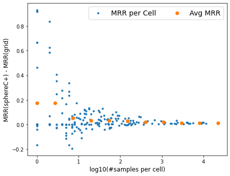
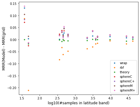
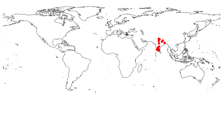
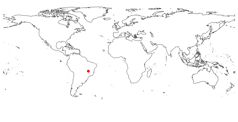
In order to further understand the reason for the superiority of $\modelname$ , we use iNat2017 and iNat2018 to conduct multiple analysis since they are the most up-to-date and have better coverage among these five datasets. Figure 3(a) shows the image locations in iNat2017 validation dataset. We split this dataset into different latitude bands and compare the $\Delta MRR$ between each model to $grid$. Figure 3(b) and 3(c) show the number of samples and $\Delta MRR$ in each band while Figure 3(f) shows that the contrast between these two variables for different models. We can clearly see that 4 $\modelname$  have larger $\Delta MRR$ are the North Pole (See Figure 3(c)). Moveover, $\modelname$  has advantages on bands with less data samples, e.g. $\phi\in[-30^{\circ},-20^{\circ})$. To have more concrete understanding, we compare $sphereC+$ and $grid$ in a higher spatial resolution - in latitude-longitude cells - which can be seen in Figure 3(d) and 3(e). We can see that $sphereC+$ have more advantages over $grid$ in North Pole and data sparse cells.

(a) Validation Locations

(b) Samples per $\phi$ band

(c) $\Delta MRR$ per $\phi$ band

(d) $\Delta MRR$ per cell

(e) $\Delta MRR$ per cell

(f) $\Delta MRR$ per $\phi$ band

Figure 3: iNat2017 dataset and model performance comparison: (a) Sample locations for validation set where the dashed and solid lines indicates latitudes; (b) The number of training and validation samples in different latitude intervals. (c) $MRR$ difference between a model and baseline $grid$ on the validation dataset. (d) $\Delta MRR=MRR(sphereC+)-MRR(grid)$ for each latitude-longitude cell. Red and blue color indicates positive and negative $\Delta MRR$ while darker color means high absolute value. The number on each cell indicates the number of validation data points while "1K+" means there are more than 1K points in a cell. (e) The number of validation samples v.s. $\Delta MRR=MRR(sphereC+)-MRR(grid)$ per latitude-longitude cell. The orange dots represent moving averages. (b) The number of validation samples v.s. $\Delta MRR$ per latitude band.

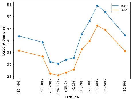
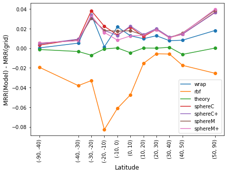
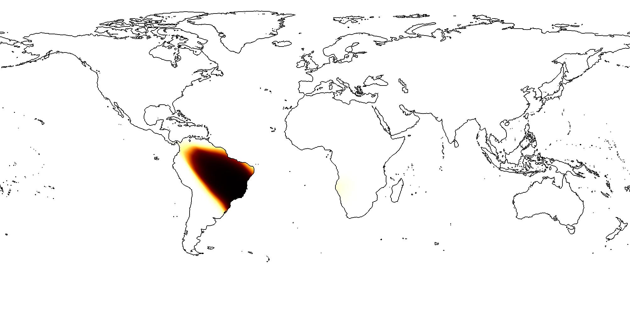
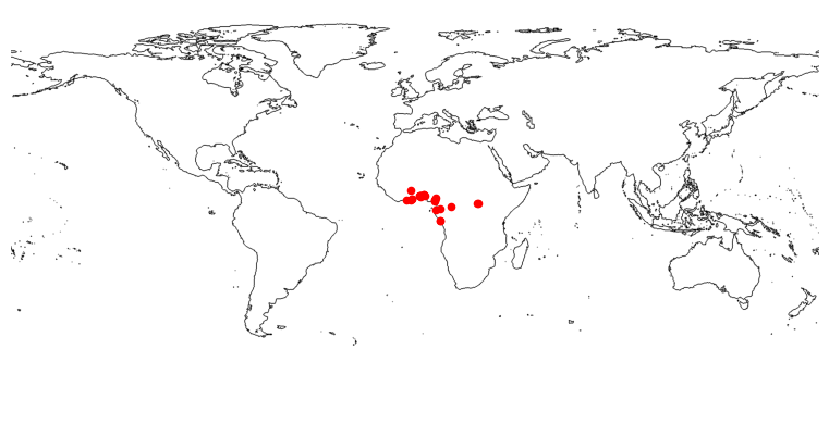
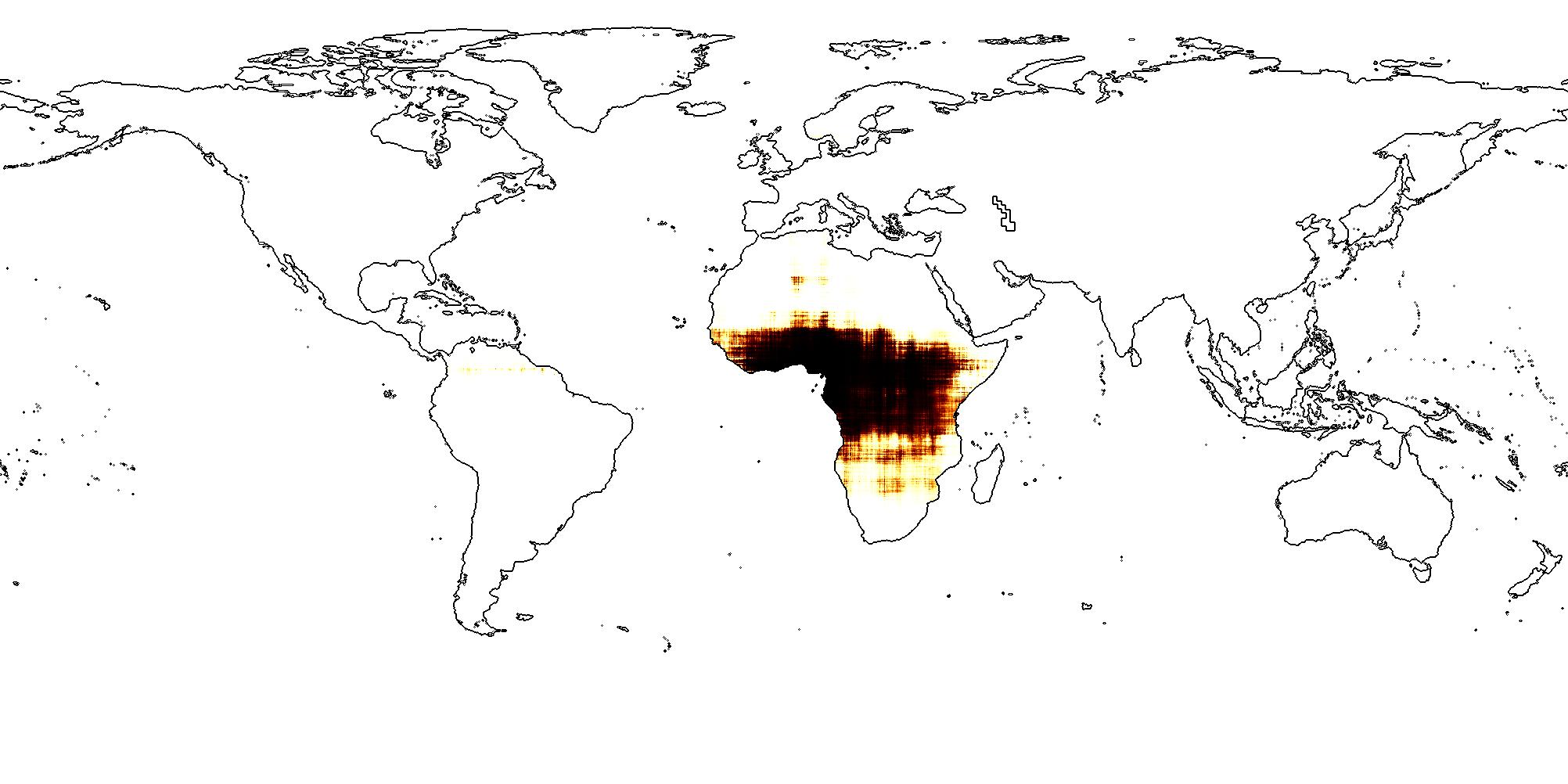
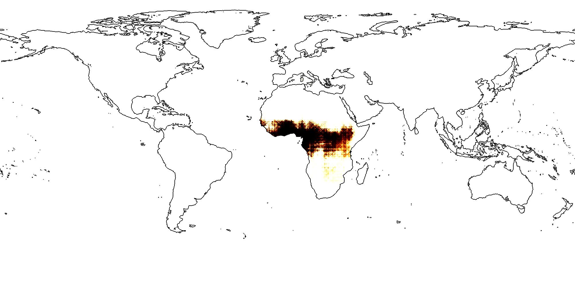
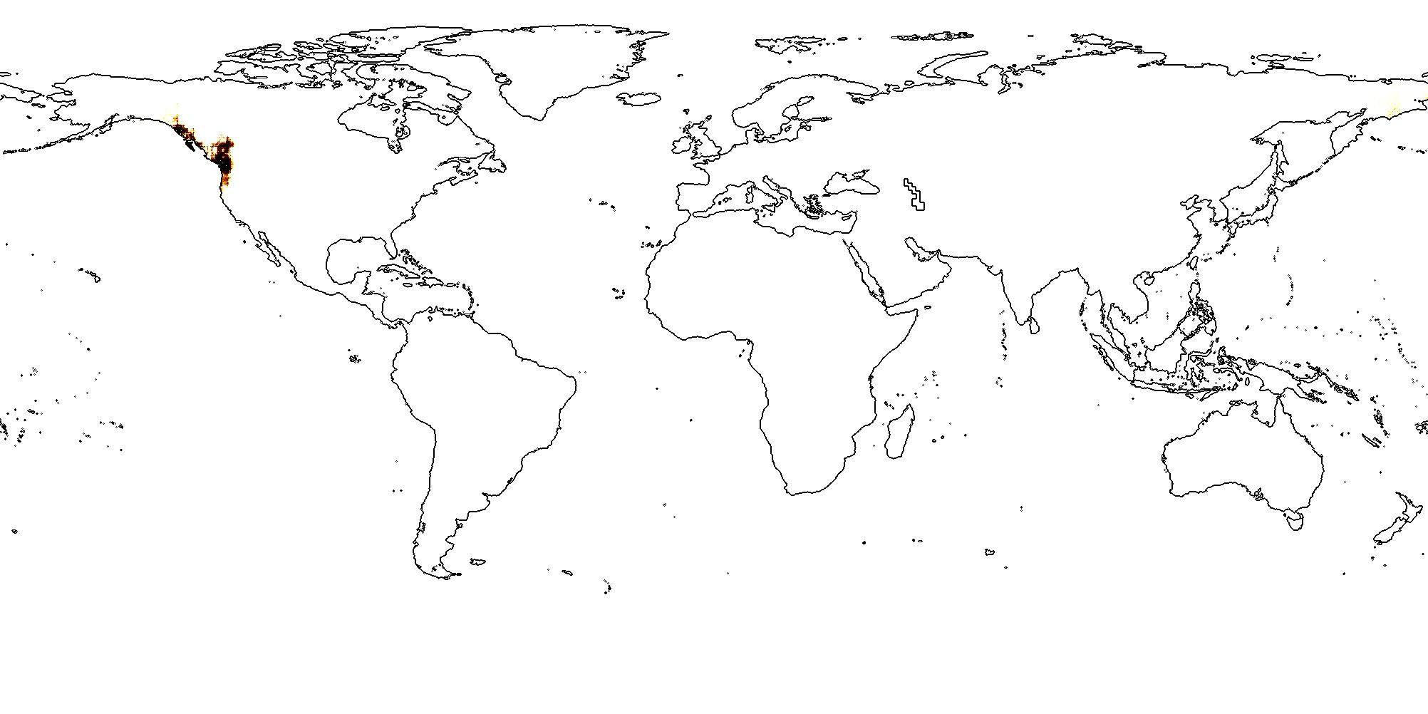
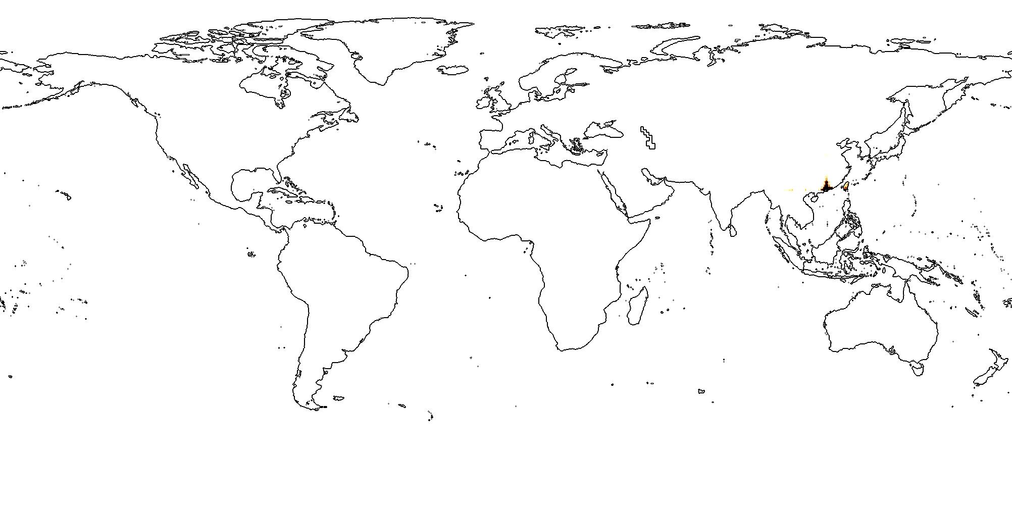
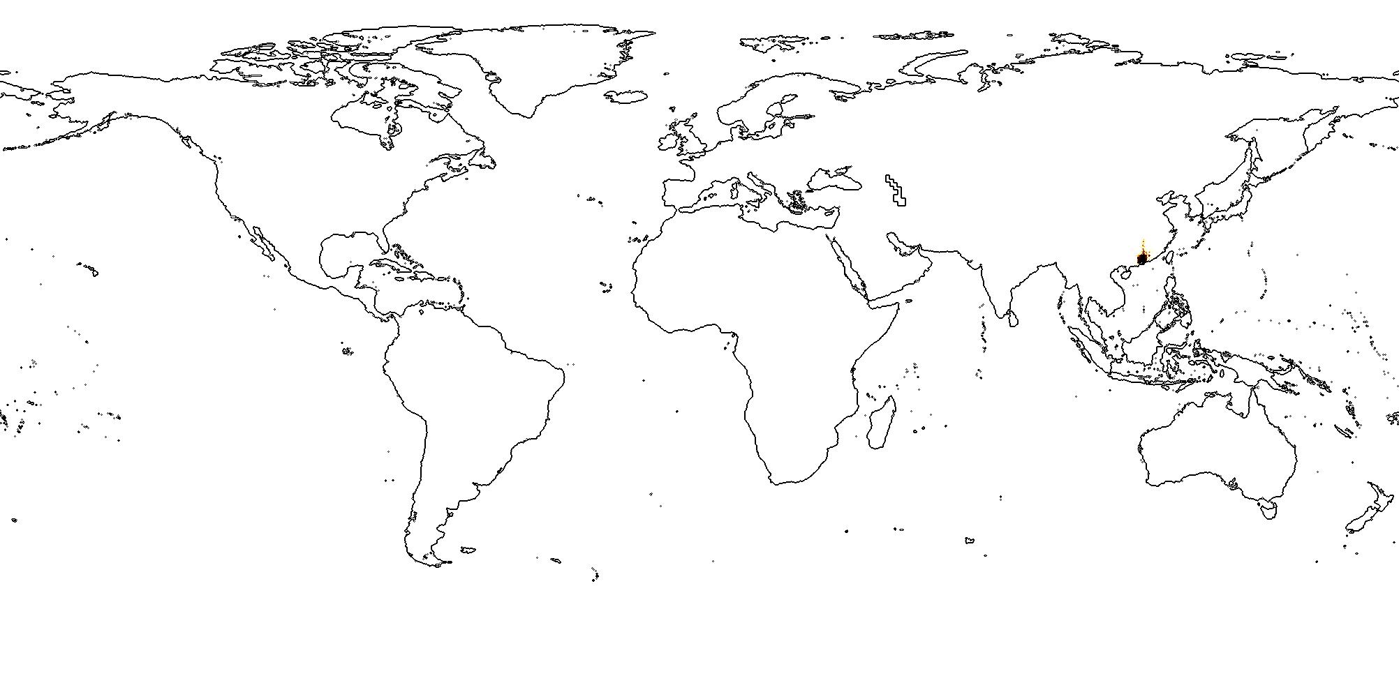
We further plot the predicted species distributions from different models at different geographic regions, and compare them with the training sample locations of the corresponding species, see Figure 1b-e and 4. We can see that compared with $wrap*$ and $grid$, in each geographic region with sparse training samples and the North Pole area, the spatial distributions produced by $sphereC+$ are more compact while the other two have over-generalization issue. For more analysis, please refer to Appendix 9.4, 9.5, and 9.6.

(a) Motacilla maderaspatensis

(b) $wrap*$

(c) $grid$

(d) $sphereC+$

(e) Siderone galanthis

(f) $wrap*$

(g) $grid$

(h) $sphereC+$

(i) Lophoceros fasciatus

(j) $wrap*$

(k) $grid$

(l) $sphereC+$

Figure 4: Compare the predicted distributions of example species from different models. The first figure of each row marks the data points from iNat2018 training data.

7 Conclusion

In this work, we propose a general purpose multi-scale spherical location encoder - $\modelname$ which can encode any location on the spherical surface into a high dimension vector which is learning-friendly for downstream neuron network models. We provide theoretical proof that $\modelname$ is able to preserve the spherical surface distance between points. We conduct experiments on the geo-aware image classification with 5 large-scale real-world datasets. Results shows that $\modelname$ can outperform the state-of-the-art 2D location encoders on both tasks. Further analysis shows that $\modelname$ is especially excel at polar regions as well data-sparse areas.

8 Broader Impact

Encoding point-features on a spherical surface is a fundamental problem, especially in geoinformatics, geography, meteorology, oceanography, geoscience, and environmental science. Our proposed $\modelname$ is a general-purpose spherical-distance-reserving encoding which can be utilized in a wide range of geospatial prediction tasks. Except for the tasks we discussed above, the potential applications include areas like public health, epidemiology, agriculture, economy, ecology, and environmental engineering, and researches like large-scale human mobility and trajectory prediction [39], geographic question answering[23], global biodiversity hotspot prediction [28, 13, 6], weather forecasting and climate change [15], global pandemic study and its relation to air pollution [38], and so on. In general, we expect our proposed $\modelname$ will benefit various AI for social goods applications which involves predictive modeling at global scales.

9 Appendix

9.1 The Map Projection Distortion Problem

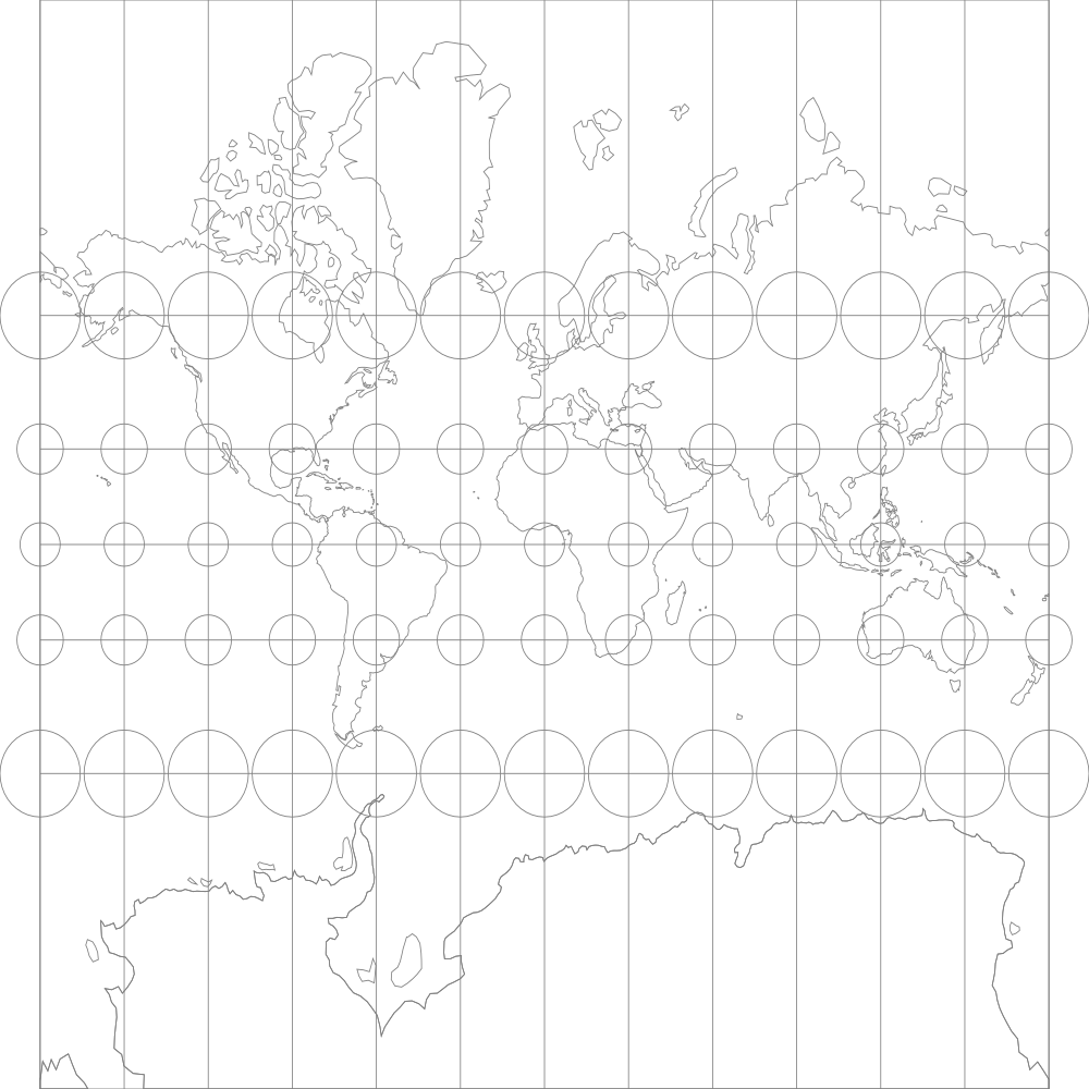
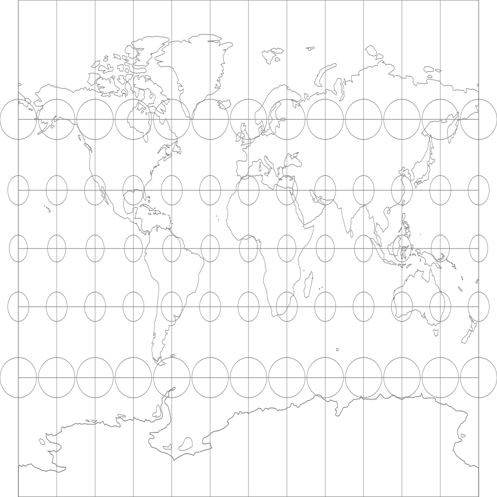
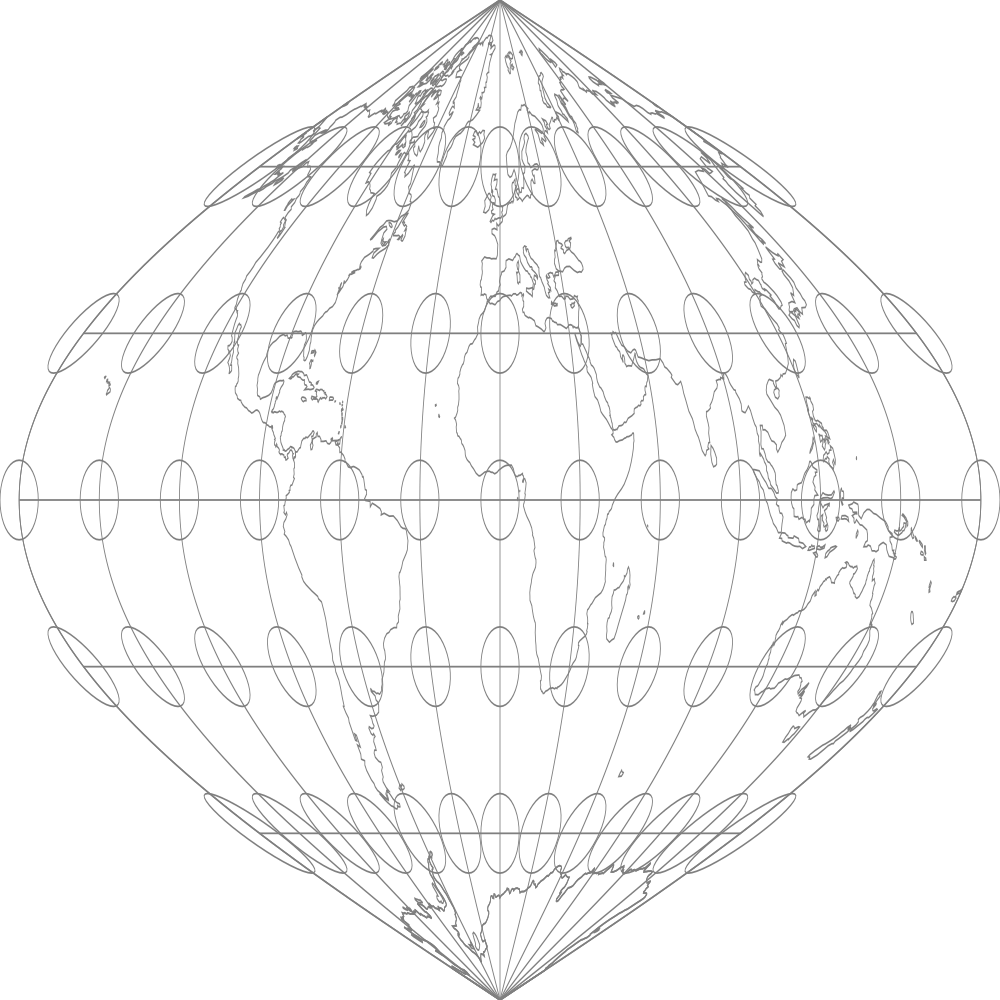
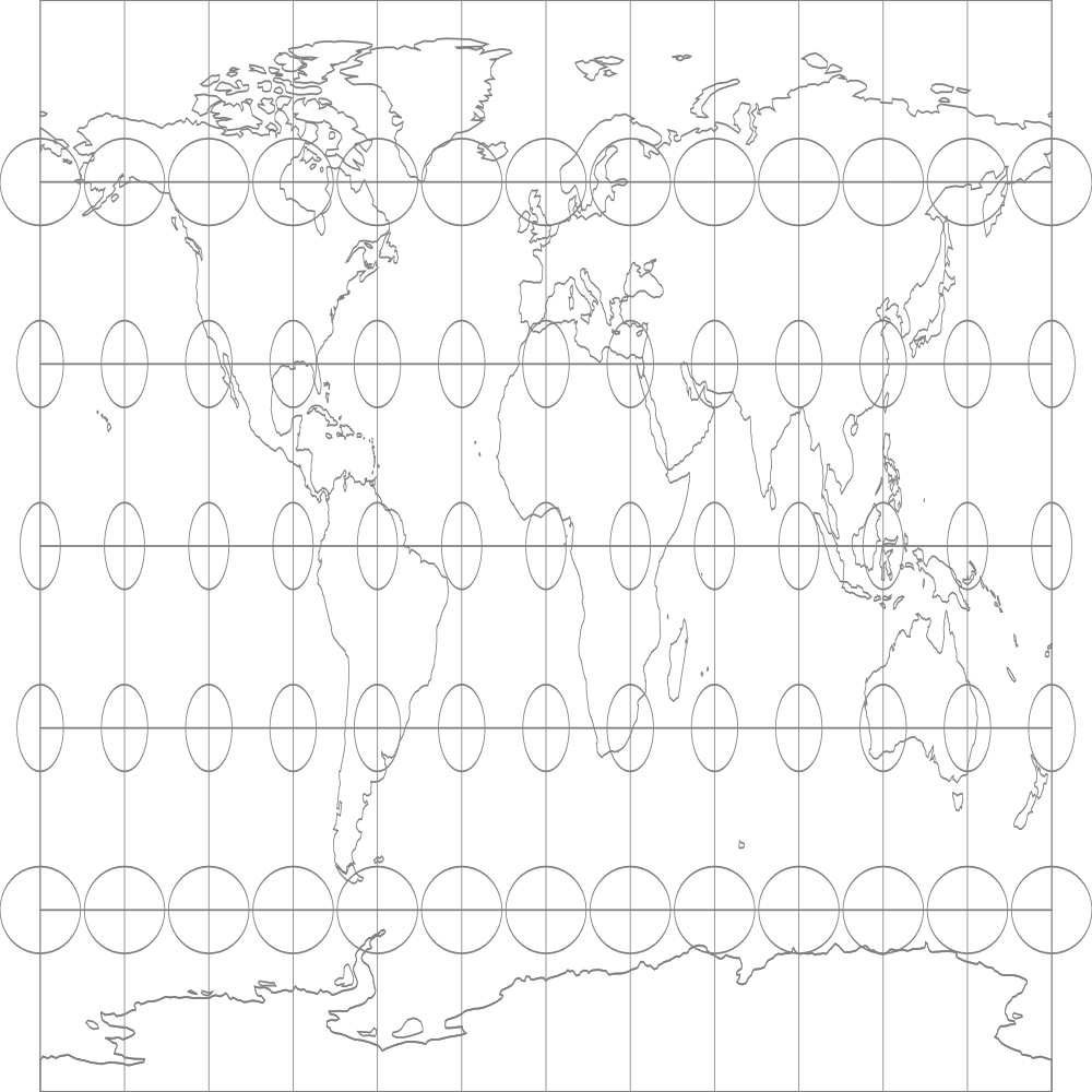
Map projection distortion is unavoidable when projecting spherical coordinates into 2D space. There are no map projection can preserve distances at all direction. The so-called equidistant projection can only preserve distance on one direction, e.g., the longitude direction for the equirectangular projection (See Figure 5(d)), while the conformal map projections (See Figure 5(a)) can preserve directions while resulting in a large distance distortion. For a comprehensive overview of map projections and their distortions, See Mulcahy et al. [27]. This is a well recognized problem in Cartography which shows the importance of calculating on a round planet [8].

(a) Mercator

(b) Miller

(c) Sinusoidal

(d) Equirectangular

Figure 5: An illustration for map projection distortion: (a)-(d): Tissot indicatrices for four projections. The equal area circles are putted in different locations to show how the map distortion affect its shape.

9.2 A Brief Overview of Geo-Aware Image Classification Task

If we assume $\mathbf{I}$ and $\boldsymbol{\mathbf{x}}$ are conditionally independent given $y$, then based on Bayes’ theorem, we have

$$P(y|\mathbf{I},\boldsymbol{\mathbf{x}})=\dfrac{P(\mathbf{I},\boldsymbol{\mathbf{x}}|y)P(y)}{P(\mathbf{I},\boldsymbol{\mathbf{x}})}=\dfrac{P(\mathbf{I}|y)P(\mathbf{I})}{P(y)}\dfrac{P(y|\boldsymbol{\mathbf{x}})P(\boldsymbol{\mathbf{x}})}{P(y)}\dfrac{P(y)}{P(\mathbf{I},\boldsymbol{\mathbf{x}})}\;\propto\;P(y|\boldsymbol{\mathbf{x}})P(y|\mathbf{I})$$ (18)

Fig 1(a) illustrates the whole workflow. The major objective for this task is to learn a geographic prior distribution $P(y|\boldsymbol{\mathbf{x}})\;\propto\;\sigma(Enc(\boldsymbol{\mathbf{x}})\mathbf{T}_{:,y})$ such that all observed species occurrences (all image locations $\boldsymbol{\mathbf{x}}$ as well as their associated species class $y$) have maximum probability. Mac Aodha et al. [21] used a loss function which is based on maximum likelihood estimation (MLE). Given a set of training samples - data points and their associated class labels $\mathbb{X}=\{(\boldsymbol{\mathbf{x}},y)\}$, the loss function $\mathcal{L}^{image}(\mathbb{X})$ is defined as:

$$\begin{split}\mathcal{L}^{image}(\mathbb{X})=\sum_{(\boldsymbol{\mathbf{x}},y)\in\mathbb{X}}\sum_{\boldsymbol{\mathbf{x}}^{-}\in\mathcal{N}(\boldsymbol{\mathbf{x}})}\Big{(}&\beta\log(\sigma(Enc(\boldsymbol{\mathbf{x}})\mathbf{T}_{:,y}))+\\ &\sum_{i=1,i\neq y}^{c}\log(1-\sigma(Enc(\boldsymbol{\mathbf{x}})\mathbf{T}_{:,i}))+\\ &\sum_{i=1}^{c}\log(1-\sigma(Enc(\boldsymbol{\mathbf{x}}^{-})\mathbf{T}_{:,i}))\Big{)}\end{split}$$ (19)

Here, $\beta$ is a hyperparameter to enlarge the weight of positive samples. $\mathcal{N}(\boldsymbol{\mathbf{x}})$ represents the negative sample set of point $\boldsymbol{\mathbf{x}}$ while $\boldsymbol{\mathbf{x}}^{-}\in\mathcal{N}(\boldsymbol{\mathbf{x}})$ is a negative sample uniformly generated from the spherical surface given each data point $\boldsymbol{\mathbf{x}}$. We follow the same model set up but replace the $wrap$ location encoder with our $\modelname$ model.

9.3   Hyperparameters

Table 2 shows the best hyperparameter combinations of different $\modelname$ models on different image classification dataset. We use a smaller $S$ for $sphereDFS$ since it has $O(S^{2})$ terms while the other models have $O(S)$ terms. $sphereDFS$ with $S=8$ yield a similar number of terms to the other models wth $S=32$ (See Table 3). Interestingly, all first four $\modelname$ models ($sphereC$, $sphereC+$, $sphereM$, and $sphereM+$) shows the best performance on all five datasets with the same hyperparamter combinations. Note that compared with other datasets, iNat2017 and iNat2018 are more up-to-date datasets with more training samples and better geographic coverage. This indicates that the proposed 4 $\modelname$ models show similar performance over different hyperparameter combinations.

Table 2: The best hyperparameter combinations of $\modelname$ models on different image classification datasets. The learning rate $lr$ tends to be smaller for larger datasets; We fix the total number of frequencies $S$ to be 8 for $sphereDFS$ and 32 for all others; the maximum scale $r_{max}=1$; $r_{min}$: the minimum scale; the number of hidden layers $\mathbf{NN}()$ is fixed to $h=1$; the number of neurons in $\mathbf{NN}()$ is fixed to $k=1024$ except for the smallest dataset.

Dataset	$lr$	$r_{min}$	$k$
BirdSnap	0.001	$10^{-6}$	512
BirdSnap$\dagger$	0.001	$10^{-4}$	1024
NABirds$\dagger$	0.001	$10^{-4}$	1024
iNat2017	0.0001	$10^{-2}$	1024
iNat2018	0.0005	$10^{-3}$	1024

Table 3: Dimension of position encoding for different models in terms of total scales $S$

Model	$sphereC$	$sphereC+$	$sphereM$	$sphereM+$	$sphereDFS$
Dimension	$3S$	$6S$	$5S$	$8S$	$4S^{2}+4S$

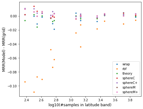
9.4 Impact of MRR by The Number of Samples at Different Latitude Bands

See Figure 6

(a) iNat2017

(b) iNat2018

Figure 6: Impact of MRR by The Number of Samples at Different Latitude Bands.

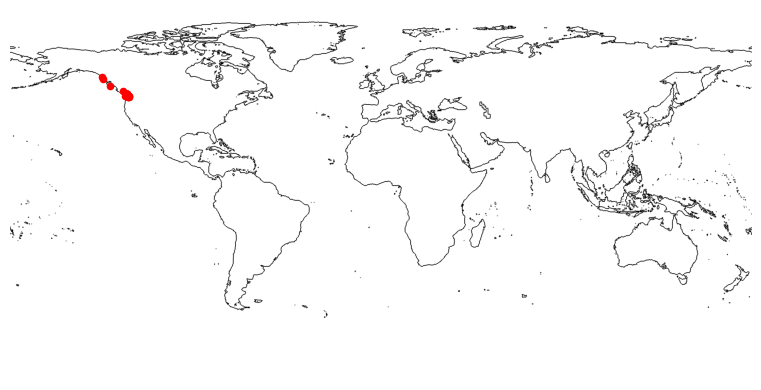
9.5 Predicted Distributions iNat2018

See Figure 7

(a) Eudistylia vancouveri

(b) $wrap*$

(c) $grid$

(d) $sphereC+$

(e) Motacilla maderaspatensis

(f) $wrap*$

(g) $grid$

(h) $sphereC+$

(i) Vulpes lagopus

(j) $wrap*$

(k) $grid$

(l) $sphereC+$

(m) Siderone galanthis

(n) $wrap*$

(o) $grid$

(p) $sphereC+$

(q) Lophoceros fasciatus

(r) $wrap*$

(s) $grid$

(t) $sphereC+$

(u) Dysphania militaris

(v) $wrap*$

(w) $grid$

(x) $sphereC+$

Figure 7: Compare the predicted distributions of example species from different models. The first figure of each row marks the data points from iNat2018 training data.

9.6 Embedding Clustering

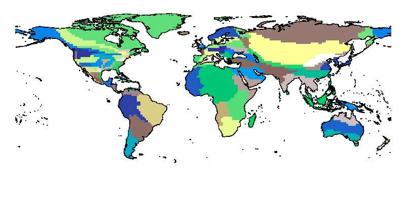
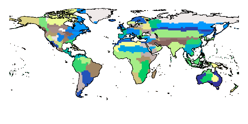
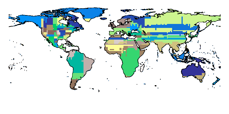
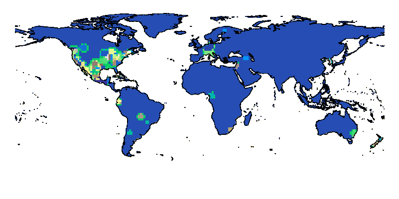
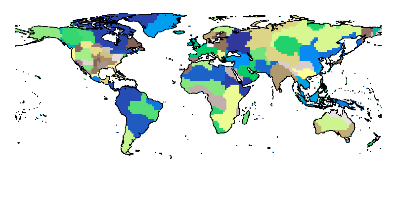
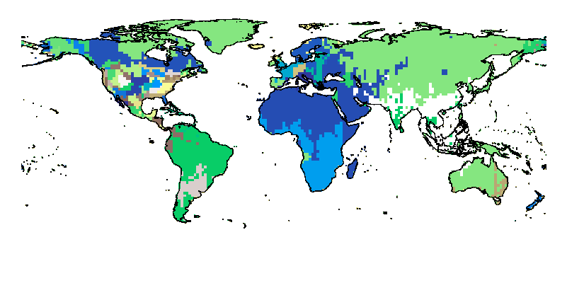
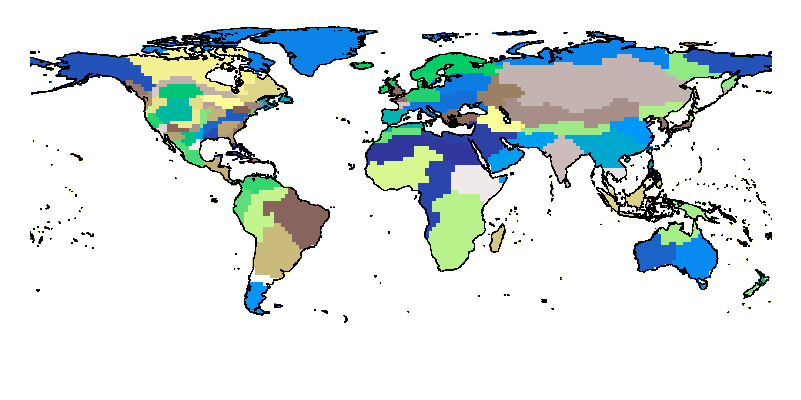
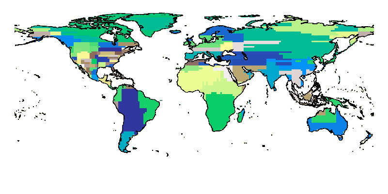
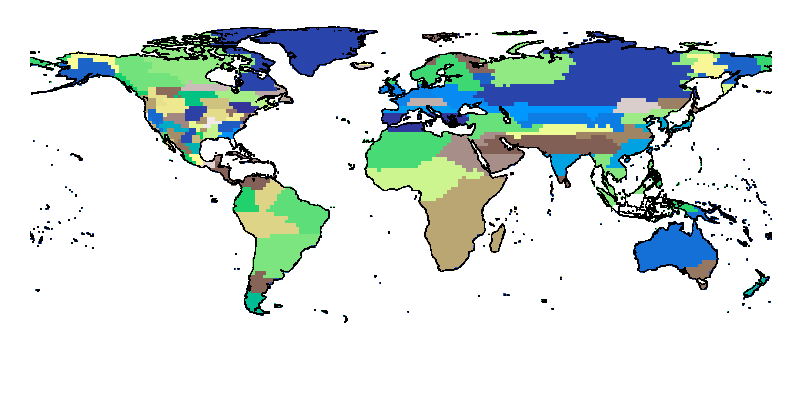
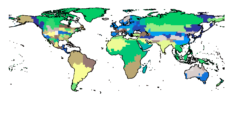
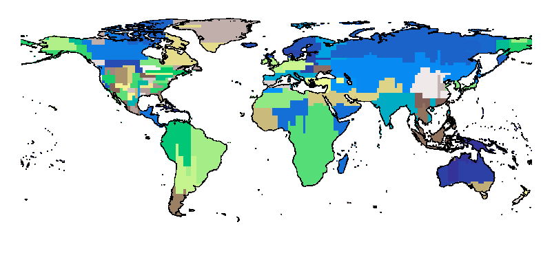
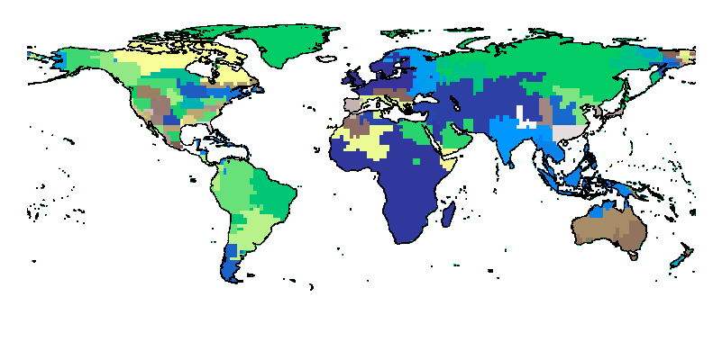
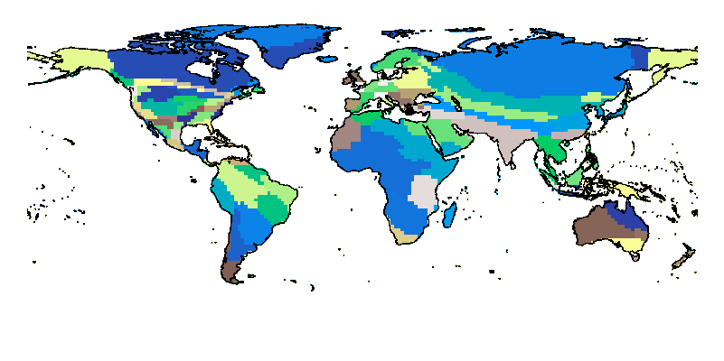
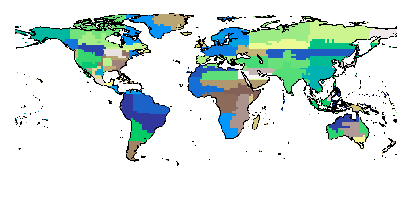
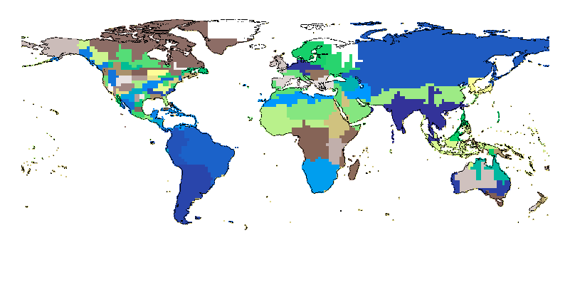
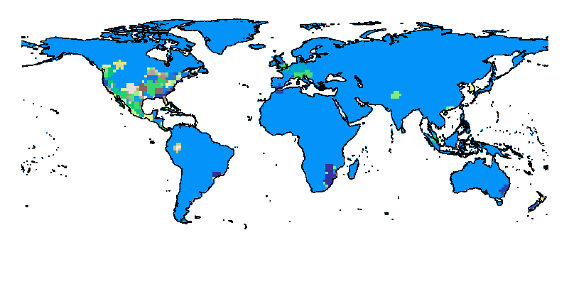
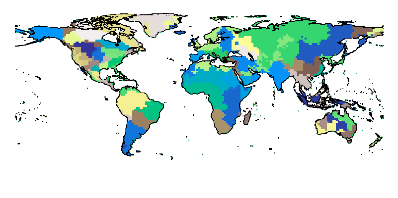
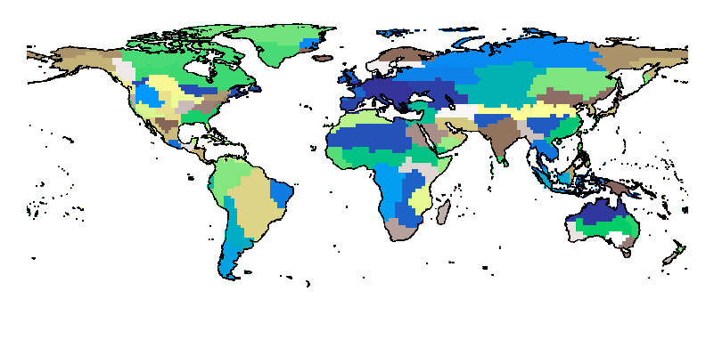
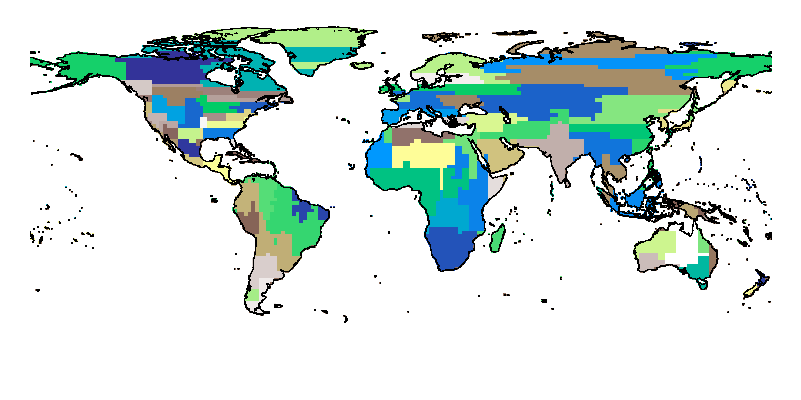
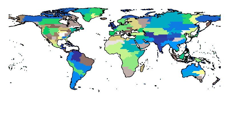
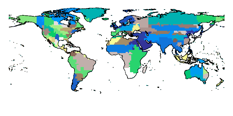
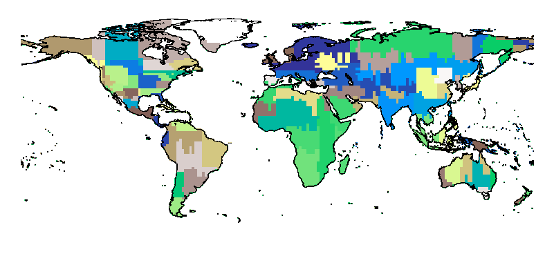
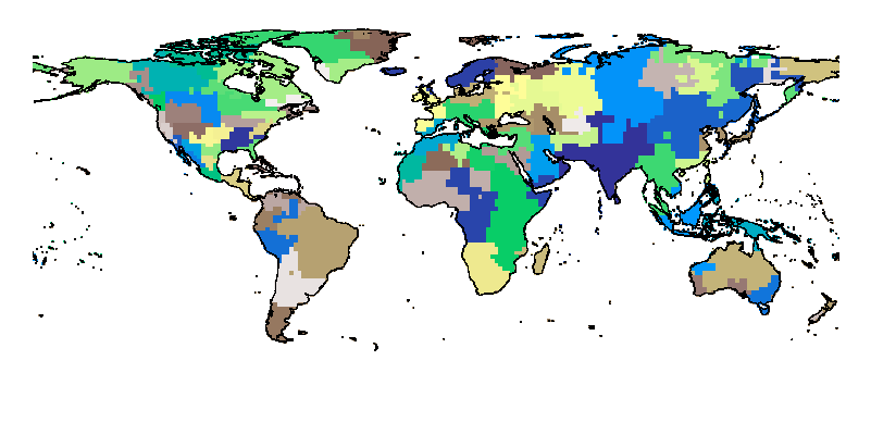
We use the location encoder trained on iNat2017 or iNat2018 dataset to produce a location embedding for the center of each small latitude-longitude cell. Then we do agglomerative clustering on all these embeddings to produce a clustering map. Figure 8 and 9 show the clustering results for different models with different hyperparameters on iNat2017 and iNat2018 dataset.

(a) $wrap*$

(b) $grid$ $(r_{min}=10^{-2})$

(c) $grid$ $(r_{min}=10^{-6})$

(d) $rbf$ $(\sigma=1,m=200)$

(e) $theory$ $(r_{min}=10^{-2})$

(f) $theory$ $(r_{min}=10^{-6})$

(g) $sphereM$ $(r_{min}=10^{-1})$

(h) $sphereM$ $(r_{min}=10^{-2})$

(i) $sphereC$ $(r_{min}=10^{-2})$

(j) $sphereC+$ $(r_{min}=10^{-2})$

(k) $sphereM+$ $(r_{min}=10^{-2})$

(l) $sphereDFS$ $(r_{min}=10^{-2})$

Figure 8: Embedding clusterings of iNat2017 models. (a) $wrap*$ with 4 hidden ReLU layers of 256 neurons; (d) $rbf$ with the best kernel size $\sigma=1$ and number of anchor points $m=200$; (b)(c)(e)(f) are $Space2Vec$ models [25] with different min scale $r_{min}=\{10^{-6},10^{-2}\}$.^a (g)-(l) are different $\modelname$ models.^b

^a They share the same best hyperparameters: $S=64$, $r_{max}=1$, and 1 hidden ReLU layers of 512 neurons.
^bThey share the same best hyperparameters: $S=32$, $r_{max}=1$, and 1 hidden ReLU layers of 1024 neurons.

(a) $wrap*$

(b) $grid$ $(r_{min}=10^{-3})$

(c) $grid$ $(r_{min}=10^{-6})$

(d) $rbf$ $(\sigma=1,m=200)$

(e) $theory$ $(r_{min}=10^{-3})$

(f) $theory$ $(r_{min}=10^{-6})$

(g) $sphereM$ $(r_{min}=10^{-1})$

(h) $sphereM$ $(r_{min}=10^{-3})$

(i) $sphereC$ $(r_{min}=10^{-3})$

(j) $sphereC+$ $(r_{min}=10^{-3})$

(k) $sphereM+$ $(r_{min}=10^{-3})$

(l) $sphereDFS$ $(r_{min}=10^{-3})$

Figure 9: Embedding clusterings of iNat2018 models. (a) $wrap*$ with 4 hidden ReLU layers of 256 neurons; (d) $rbf$ with the best kernel size $\sigma=1$ and number of anchor points $m=200$; (b)(c)(e)(f) are $Space2Vec$ models [25] with different min scale $r_{min}=\{10^{-6},10^{-3}\}$.^a (g)-(l) are $\modelname$ models with different min scale.^b

^a They share the same best hyperparameters: $S=64$, $r_{max}=1$, and 1 hidden ReLU layers of 512 neurons.
^bThey share the same best hyperparameters: $S=32$, $r_{max}=1$, and 1 hidden ReLU layers of 1024 neurons.

References

- [1] Andrea Banino, Caswell Barry, Benigno Uria, Charles Blundell, Timothy Lillicrap, Piotr Mirowski, Alexander Pritzel, Martin J Chadwick, Thomas Degris, Joseph Modayil, et al. Vector-based navigation using grid-like representations in artificial agents. Nature, 557(7705):429, 2018.
- [2] Robert Bartnik and Andrew Norton. Numerical methods for the einstein equations in null quasi-spherical coordinates. SIAM Journal on Scientific Computing, 22:917–950, 03 2000.
- [3] Thomas Berg, Jiongxin Liu, Seung Woo Lee, Michelle L Alexander, David W Jacobs, and Peter N Belhumeur. Birdsnap: Large-scale fine-grained visual categorization of birds. In Proceedings of the IEEE Conference on Computer Vision and Pattern Recognition, pages 2011–2018, 2014.
- [4] Michael M Bronstein, Joan Bruna, Yann LeCun, Arthur Szlam, and Pierre Vandergheynst. Geometric deep learning: going beyond euclidean data. IEEE Signal Processing Magazine, 34(4):18–42, 2017.
- [5] Cyril Caminade, Sari Kovats, Joacim Rocklov, Adrian M. Tompkins, Andrew P. Morse, Felipe J. Colón-González, Hans Stenlund, Pim Martens, and Simon J. Lloyd. Impact of climate change on global malaria distribution. Proceedings of the National Academy of Sciences, 111(9):3286–3291, 2014.
- [6] Gerardo Ceballos, Paul R. Ehrlich, and Peter H. Raven. Vertebrates on the brink as indicators of biological annihilation and the sixth mass extinction. Proceedings of the National Academy of Sciences, 2020.
- [7] Matteo Chinazzi, Jessica T. Davis, Marco Ajelli, Corrado Gioannini, Maria Litvinova, Stefano Merler, Ana Pastore y Piontti, Kunpeng Mu, Luca Rossi, Kaiyuan Sun, Cécile Viboud, Xinyue Xiong, Hongjie Yu, M. Elizabeth Halloran, Ira M. Longini, and Alessandro Vespignani. The effect of travel restrictions on the spread of the 2019 novel coronavirus (covid-19) outbreak. Science, 368(6489):395–400, 2020.
- [8] Nicholas R Chrisman. Calculating on a round planet. International Journal of Geographical Information Science, 31(4):637–657, 2017.
- [9] Grace Chu, Brian Potetz, Weijun Wang, Andrew Howard, Yang Song, Fernando Brucher, Thomas Leung, and Hartwig Adam. Geo-aware networks for fine-grained recognition. In Proceedings of the IEEE International Conference on Computer Vision Workshops, pages 0–0, 2019.
- [10] Taco S Cohen, Mario Geiger, Jonas Köhler, and Max Welling. Spherical CNNs. In Proceedings of ICLR 2018, 2018.
- [11] Benjamin Coors, Alexandru Paul Condurache, and Andreas Geiger. SphereNet: Learning spherical representations for detection and classification in omnidirectional images. In Proceedings of the European Conference on Computer Vision (ECCV), pages 518–533, 2018.
- [12] Christopher J Cueva and Xue-Xin Wei. Emergence of grid-like representations by training recurrent neural networks to perform spatial localization. In Proceedings of ICLR 2018, 2018.
- [13] Moreno Di Marco, Simon Ferrier, Tom D. Harwood, Andrew J. Hoskins, and James E. M. Watson. Wilderness areas halve the extinction risk of terrestrial biodiversity. Nature, 573(7775):582–585, 2019.
- [14] Ruiqi Gao, Jianwen Xie, Song-Chun Zhu, and Ying Nian Wu. Learning grid cells as vector representation of self-position coupled with matrix representation of self-motion. In Proceedings of ICLR 2019, 2019.
- [15] Yoo-Geun Ham, Jeong-Hwan Kim, and Jing-Jia Luo. Deep learning for multi-year enso forecasts. Nature, 573(7775):568–572, 2019.
- [16] Gerrit Hansen and Wolfgang Cramer. Global distribution of observed climate change impacts. Nature Climate Change, 5(3):182–185, 2015.
- [17] Mike Izbicki, Evangelos E Papalexakis, and Vassilis J Tsotras. Exploiting the earth’s spherical geometry to geolocate images. In Joint European Conference on Machine Learning and Knowledge Discovery in Databases, pages 3–19. Springer, 2019.
- [18] Mike Izbicki, Vagelis Papalexakis, and Vassilis Tsotras. Geolocating tweets in any language at any location. In Proceedings of the 28th ACM International Conference on Information and Knowledge Management, pages 89–98, 2019.
- [19] Krzysztof Janowicz, Song Gao, Grant McKenzie, Yingjie Hu, and Budhendra Bhaduri. GeoAI: Spatially explicit artificial intelligence techniques for geographic knowledge discovery and beyond, 2020.
- [20] Mayank Kejriwal and Pedro Szekely. Neural embeddings for populated geonames locations. In International Semantic Web Conference, pages 139–146. Springer, 2017.
- [21] Oisin Mac Aodha, Elijah Cole, and Pietro Perona. Presence-only geographical priors for fine-grained image classification. In Proceedings of the IEEE International Conference on Computer Vision, pages 9596–9606, 2019.
- [22] Gengchen Mai. Geographic Question Answering with Spatially-Explicit Machine Learning Models. PhD thesis, UC Santa Barbara, 2021.
- [23] Gengchen Mai, Krzysztof Janowicz, Ling Cai, Rui Zhu, Blake Regalia, Bo Yan, Meilin Shi, and Ni Lao. SE-KGE: A location-aware knowledge graph embedding model for geographic question answering and spatial semantic lifting. Transactions in GIS, 2020.
- [24] Gengchen Mai, Krzysztof Janowicz, Yingjie Hu, Song Gao, Bo Yan, Rui Zhu, Ling Cai, and Ni Lao. A review of location encoding for geoai: Methods and applications. arXiv preprint arXiv:2111.04006, 2021.
- [25] Gengchen Mai, Krzysztof Janowicz, Bo Yan, Rui Zhu, Ling Cai, and Ni Lao. Multi-scale representation learning for spatial feature distributions using grid cells. In The Eighth International Conference on Learning Representations. openreview, 2020.
- [26] Philip E. Merilees. The pseudospectral approximation applied to the shallow water equations on a sphere. Atmosphere, 11(1):13–20, 1973.
- [27] Karen A Mulcahy and Keith C Clarke. Symbolization of map projection distortion: a review. Cartography and geographic information science, 28(3):167–182, 2001.
- [28] Norman Myers, Russell A Mittermeier, Cristina G Mittermeier, Gustavo AB Da Fonseca, and Jennifer Kent. Biodiversity hotspots for conservation priorities. Nature, 403(6772):853, 2000.
- [29] Steven A. Orszag. Comparison of pseudospectral and spectral approximation. Appl. Math., 51:253–259, 1972.
- [30] Steven A. Orszag. Fourier series on spheres. Mon. Wea. Rev., 102:56–75, 1974.
- [31] Bernhard Schölkopf. The kernel trick for distances. In Advances in Neural Information Processing Systems, pages 301–307, 2001.
- [32] Cheng Sun, Jianping Li, Fei-Fei Jin, and Fei Xie. Contrasting meridional structures of stratospheric and tropospheric planetary wave variability in the northern hemisphere. Tellus A: Dynamic Meteorology and Oceanography, 66(1):25303, 2014.
- [33] Christian Szegedy, Vincent Vanhoucke, Sergey Ioffe, Jon Shlens, and Zbigniew Wojna. Rethinking the inception architecture for computer vision. In Proceedings of the IEEE conference on computer vision and pattern recognition, pages 2818–2826, 2016.
- [34] Kevin Tang, Manohar Paluri, Li Fei-Fei, Rob Fergus, and Lubomir Bourdev. Improving image classification with location context. In Proceedings of the IEEE international conference on computer vision, pages 1008–1016, 2015.
- [35] Ashish Vaswani, Noam Shazeer, Niki Parmar, Jakob Uszkoreit, Llion Jones, Aidan N Gomez, Łukasz Kaiser, and Illia Polosukhin. Attention is all you need. In Advances in Neural Information Processing Systems, pages 5998–6008, 2017.
- [36] Tobias Weyand, Ilya Kostrikov, and James Philbin. Planet-photo geolocation with convolutional neural networks. In European Conference on Computer Vision, pages 37–55. Springer, 2016.
- [37] David Williamson and Gerald Browning. Comparison of grids and difference approximations for numerical weather prediction over a sphere. Journal of Applied Meteorology, 12:264–274, 02 1973.
- [38] Xiao Wu, Rachel C Nethery, Benjamin M Sabath, Danielle Braun, and Francesca Dominici. Exposure to air pollution and covid-19 mortality in the united states. medRxiv, 2020.
- [39] Yanyu Xu, Zhixin Piao, and Shenghua Gao. Encoding crowd interaction with deep neural network for pedestrian trajectory prediction. In Proceedings of the IEEE Conference on Computer Vision and Pattern Recognition, pages 5275–5284, 2018.
- [40] Bo Yan, Krzysztof Janowicz, Gengchen Mai, and Rui Zhu. A spatially-explicit reinforcement learning model for geographic knowledge graph summarization. Transactions in GIS, 2019.
- [41] Ellen D Zhong, Tristan Bepler, Joseph H Davis, and Bonnie Berger. Reconstructing continuous distributions of 3d protein structure from cryo-em images. In International Conference on Learning Representations, 2020.