Multi-agent Performative Prediction: From Global Stability and Optimality to Chaos111This research-project is supported in part by the National Research Foundation, Singapore under NRF 2018 Fellowship NRF-NRFF2018-07, AI Singapore Program (AISG Award No: AISG2-RP-2020-016), NRF2019-NRF-ANR095 ALIAS grant, AME Programmatic Fund (Grant No. A20H6b0151) from the Agency for Science, Technology and Research (A*STAR), grant PIE-SGP-AI-2018-01 and Provost’s Chair Professorship grant RGEPPV2101.

Georgios Piliouras SUTD, georgios@sutd.edu.sg    Fang-Yi Yu Harvard University, fangyiyu@seas.harvard.edu
Abstract

The recent framework of performative prediction [28] is aimed at capturing settings where predictions influence the target/outcome they want to predict. In this paper, we introduce a natural multi-agent version of this framework, where multiple decision makers try to predict the same outcome. We showcase that such competition can result in interesting phenomena by proving the possibility of phase transitions from stability to instability and eventually chaos. Specifically, we present settings of multi-agent performative prediction where under sufficient conditions their dynamics lead to global stability and optimality. In the opposite direction, when the agents are not sufficiently cautious in their learning/updates rates, we show that instability and in fact formal chaos is possible. We complement our theoretical predictions with simulations showcasing the predictive power of our results.

1 Introduction

Performative prediction [28] is a recently introduced framework that focuses on a natural but largely unexplored element of supervised learning. In many practical cases the predictive model can affect the very outcome that it is trying to predict. For example, predictions about which part of a road network will have high congestion trigger responses from the drivers which affect the resulting traffic realization leading to a shift of the target distribution. In such settings, [28] explored conditions for the existence and approximate optimality of stable equilibria of such processes.

One possible way to interpret the performative prediction setting is a single agent “game”, where the predictive agent is playing a game against himself. An agent chooses the parameters of his model as his actions but the predictive accuracy/cost of the model depends on his own past actions. Fixed points of this process do not allow for profitable deviations. Once cast in this light, it becomes self-evident that the restriction to a single predictive agent/model is arguably only the first step in capturing more general phenomena where there is a closed loop between predictive models and their environment. This motivates our central question:

Question.

What is the interplay between stability, optimality in cases where multiple predictive models operate in parallel to each other? Can the competition between multiple models lead to novel phenomena such as phase transitions from stability to instability and chaos?

A natural setting to consider for example is market competition, where multiple hedge funds are trying to simultaneously predict future prices, volatility of financial instruments. Of course as they act upon their predictions they also move the prices of these commodities in a highly correlated way. As more agents enter the market and the competition becomes increasingly fierce, is it possible that at some point the market flips from quickly discovering accurate stable predictions reflecting the underlying market fundamentals to self-induced unpredictability and chaos? When it comes to performative prediction can too many cooks spoil the soup?

1.1 Our model

Standard supervised learning consists of three components: a set of predictive models, a loss function, and a data distribution. The learner (agent) observes samples of the distribution, and then decides a predictive model. When predictions are performative, the agent’s decision of a predictive model influences the data distribution. Thus, instead of a fixed data distribution, a predictive prediction also has a distribution map which is a map from the agent’s predictive models to data distributions. We further propose multi-agent performative prediction which model the influence of multiple agents’ decisions on the data distribution, and ask whether this influence leads to convergent or chaotic systems.

To understand the framework of multi-agent performative prediction, we study a natural regression problem with multi-agent location-scale distribution maps (definition 2.2) where the agents’ influence is linear in the agents’ models. Specifically, the data consist of features and outcomes. The influence of agent i[n]𝑖delimited-[]𝑛i\in[n] on the outcome distribution is his model weighted by a scalar λi>0subscript𝜆𝑖0\lambda_{i}>0. When n=1𝑛1n=1, our multi-agent location-scale distribution map is a special case of location-scale family in Miller et al. [25]. In the market example, each hedge fund company predicts the price (outcome) based on macroeconomic data or other information (features). These influence parameters λ1,,λnsubscript𝜆1subscript𝜆𝑛\lambda_{1},\dots,\lambda_{n} can be seen as each hedge fund’s capital that can influence the future price.

Moreover, the agents often cannot know the distribution map that captures the dependency between their model and the data distribution. Therefore, we consider that the agents use a reinforcement learning algorithm, exponentiated gradient for linear regression [17], to myopically and iteratively improve their predictive models in rounds. We study the long-term behavior and ask if the system converges to the performative stable and optimal point, or behaves chaotically.

1.2 Our results

We first study the basic properties of our multi-agent preformative prediction with a multi-agent location-scale distribution map. We show 1) the existence of performative stable point in our setting (LABEL:prop:existence) and 2) the performative stability and performative optimality are equivalent (LABEL:prop:stable2optimal). This equivalence allows us to focus on the dynamical behavior of the system.

In section 4, we introduce learning dynamics to the multi-agent performative prediction where the agents use reinforcement learning algorithms, and study their long-term behavior. We provide a threshold result on the learning rates of exponentiated gradient descent and the collective influence: LABEL:thm:converge shows the dynamics of exponential gradient descent converge to the performative stable and optimal point when the learning rate is small enough fixing agents’ influence parameters λ1,,λnsubscript𝜆1subscript𝜆𝑛\lambda_{1},\dots,\lambda_{n}. Our convergence result in LABEL:thm:converge holds when the feature space is multi-dimensional, and every learning agent can use different learning rates starting at arbitrarily interior states. Our exact convergence result also works in the single-agent performative prediction setting. Contrarily, previous convergent results in [28, 25, 24] only show that their dynamics converge to a small neighborhood of the performative stable point.

On the other hand, section 4.2 shows the dynamics can have chaotic behavior if the collective influence iλisubscript𝑖subscript𝜆𝑖\sum_{i}\lambda_{i} is large enough for any fixed learning rate. Specifically, LABEL:thm:chaos_one shows that even when the feature space is in 2superscript2\mathbb{R}^{2} these systems provably exhibit Li-Yorke chaos, when the collective influence iλisubscript𝑖subscript𝜆𝑖\sum_{i}\lambda_{i} is large enough. This implies that there exists an uncountable “scrambled” set so that given any two initial conditions in the set, the liminf of the distance between these two dynamics is zero, but the limsup of their distance is positive. (LABEL:def:chaos) The chaotic result in LABEL:thm:chaos_one also holds for the original single-agent performative prediction so long as the agent’s influence is large enough, and, thus, complements previous performative prediction works on convergence behavior, which primarily consider that the agent’s influence on the data distribution is sufficiently small. Moreover, no matter how small the agents’ learning rates, LABEL:thm:chaos_one shows that chaos is inevitable in some performative predictions settings when the number of agents exceeds a carrying capacity. After that, the system becomes unpredictable with small perturbations exploding exponentially fast. Though our chaotic result closely follows Chotibut et al. [10], we need a new proof for the existence of period three orbits, because the fixed point of our dynamics changes as the total influence iλisubscript𝑖subscript𝜆𝑖\sum_{i}\lambda_{i} increases.

Finally, section 5 provides numerical examples of our dynamics and shows convergent and chaotic behavior. Additionally, through simulation, we demonstrate that our convergent and chaotic results also hold when the agents can only access noisy estimation of the gradient and conduct stochastic exponentiated gradient descent.

Related work

Data distribution shift is not a new topic in ML, but earlier works focused primarily on exogenous changes to the data generating distribution. Performativity is machine learning was introduced by [28]. The original work and several follow-ups study the discrepancy between performative stability and performative optimality and prove approximated convergence of learning dynamics, e.g., stochastic gradient descent, or iterative empirical risk minimization. [24, 12, 16] Performativity of prediction is also related to several applications: strategic classification [15], retraining [4, 19].

Inspired by the instability of training algorithms in ML applications such as Generative Adversarial Networks (GANs), there has been a lot of recent interest in understanding conditions (particularly in multi-agent systems) where learning behavior may be non-equilibrating/unstable [8, 3, 13, 1, 21, 14]. The (in)stability and performance of exponentiated gradient descent in particular (also referred to as Multiplicative Weights Updates) and other closely related dynamics has attracted a lot of attention [11, 2, 6, 27, 7, 29]. The technique of Li-Yorke chaos has recently found applications across several different domains such as routing games, Cournot games and blockchain protocols [26, 10, 5, 9, 20]. To our knowledge, this is the first time where such formal chaotic results are established in settings related to performative prediction and supervised learning more generally.

Another line of related works is learning in games. Specifically, our dynamics can be seen as special cases multiplicative weight update (Hedge algorithms) on congestion games. Previous works on Hedge algorithms only show exact convergence when the learning rate is decreasing [18, 11], and, to our best knowledge, our results are the first that shows exact convergence of Hedge algorithms with small constant learning rates. Our results also complement the exact convergence result of the linear variant of multiplicative weight update by Palaiopanos et al. [26].

2 Preliminary

2.1 Multi-agent Performative Prediction

We first formulate the framework of multi-agent performative prediction, and we introduce an example of multi-agent performative prediction on which we will focus.

A multi-agent performative prediction comprises n𝑛n agents deploying their predictive models fθ1,,fθnsubscript𝑓superscript𝜃1subscript𝑓superscript𝜃𝑛f_{\theta^{1}},\dots,f_{\theta^{n}} with parameters 𝜽1,𝜽2,,𝜽nΘsuperscript𝜽1superscript𝜽2superscript𝜽𝑛Θ{\bm{\theta}}^{1},{\bm{\theta}}^{2},\dots,{\bm{\theta}}^{n}\in\Theta that collectively influence the future data distribution. We formalize such dependency via a distribution map 𝒟()𝒟\mathcal{D}(\cdot) which outputs a distribution on the data, 𝒟(𝜽)𝒟𝜽\mathcal{D}({\vec{\bm{\theta}}}), given a models profile 𝜽:=(𝜽1,,𝜽n)Θnassign𝜽superscript𝜽1superscript𝜽𝑛superscriptΘ𝑛{\vec{\bm{\theta}}}:=({\bm{\theta}}^{1},\dots,{\bm{\theta}}^{n})\in\Theta^{n}. A loss function (𝒛,𝜽)𝒛superscript𝜽\ell({\bm{z}},{\bm{\theta}}^{\prime}) measures the loss of a model f𝜽subscript𝑓superscript𝜽f_{{\bm{\theta}}^{\prime}} on a data point 𝒛𝒵𝒛𝒵{\bm{z}}\in\mathcal{Z}, and the expected loss on a distribution 𝒟𝒟\mathcal{D} is 𝔼𝐳𝒟[(𝐳,𝜽)]subscript𝔼similar-to𝐳𝒟delimited-[]𝐳superscript𝜽\mathbb{E}_{{\mathbf{z}}\sim\mathcal{D}}[\ell({\mathbf{z}},{\bm{\theta}}^{\prime})]. For performative prediction, we further define the decoupled performative loss on a distribution mapping 𝒟𝒟\mathcal{D} as

(𝜽,𝜽):=𝔼𝐳𝒟(𝜽)(𝐳,𝜽)assign𝜽superscript𝜽subscript𝔼similar-to𝐳𝒟𝜽𝐳superscript𝜽\ell({\vec{\bm{\theta}}},{\bm{\theta}}^{\prime}):=\mathbb{E}_{{\mathbf{z}}\sim\mathcal{D}({\vec{\bm{\theta}}})}\ell({\mathbf{z}},{\bm{\theta}}^{\prime})

where 𝜽Θsuperscript𝜽Θ{\bm{\theta}}^{\prime}\in\Theta denotes a predictive model, while 𝜽Θn𝜽superscriptΘ𝑛{\vec{\bm{\theta}}}\in\Theta^{n} denotes a deployed model profile.

Given the set of model ΘΘ\Theta, the loss function \ell, and the distribution mapping 𝒟𝒟\mathcal{D}, each agent in a multi-agent performative prediction (Θ,,𝒟)Θ𝒟(\Theta,\ell,\mathcal{D}) pursues minimal loss on the distribution that they collectively induce. We consider two solution concepts performative optimality and performative stability which generalizes the original ones in [28].

Definition 2.1 (label = def:stable).

Given (Θ,,𝒟)Θ𝒟(\Theta,\ell,\mathcal{D}), a models profile 𝜽Θnsuperscript𝜽superscriptΘ𝑛{\vec{\bm{\theta}}}^{*}{\in\Theta^{n}} is performatively optimal if the total loss is minimized,

𝜽argmin𝜽Θni(𝜽,𝜽i).superscript𝜽subscriptargmin𝜽superscriptΘ𝑛subscript𝑖𝜽superscript𝜽𝑖{\vec{\bm{\theta}}}^{*}\in\operatorname*{arg\,min}_{{\vec{\bm{\theta}}}{\in\Theta^{n}}}\sum_{i}\ell({\vec{\bm{\theta}}},{\bm{\theta}}^{i}).

Another desirable property of a model profile is that, given all agents deploy their models, their models are also simultaneously optimal for distribution that their model induces. Formally, 𝜽superscript𝜽{\vec{\bm{\theta}}}^{*} is performatively stable if for all i[n]𝑖delimited-[]𝑛i\in[n]

(𝜽)iargmin𝜽iΘ(𝜽,𝜽i).superscriptsuperscript𝜽𝑖subscriptargminsuperscript𝜽𝑖Θsuperscript𝜽superscript𝜽𝑖({\bm{\theta}}^{*})^{i}\in\operatorname*{arg\,min}_{{\bm{\theta}}^{i}{\in\Theta}}\ell({\vec{\bm{\theta}}}^{*},{\bm{\theta}}^{i}).

The performative optimality does not implies the performative stable point. For performative optimal point, the variable for minimization 𝜽𝜽{\vec{\bm{\theta}}} affects both the first and the second argument, but only affect the second one for performative stable point. Now we introduce our model in this paper.

Location-scale distribution map

In this paper, we study the family of multi-agent location-scale map for regression problem where a data point consists of d𝑑d-dimensional feature and scalar outcome, 𝒛=(𝒙,y)𝒛𝒙𝑦{\bm{z}}=({\bm{x}},y). In the location-scale distribution map, the performative effects is linear in 𝜽𝜽{\vec{\bm{\theta}}}.

Definition 2.2.

Given d𝑑d\in\mathbb{N} and d2𝑑2d\geq 2, and ΘndsuperscriptΘ𝑛superscript𝑑{\Theta^{n}}\subseteq\mathbb{R}^{d}, a distribution map 𝒟:Θnd×:𝒟superscriptΘ𝑛superscript𝑑\mathcal{D}:{\Theta^{n}}\to\mathbb{R}^{d}\times\mathbb{R} is a multi-agent location-scale distribution map on n𝑛n parties if there exists a static distribution 𝒟Xsubscript𝒟𝑋\mathcal{D}_{X} on d+1superscript𝑑1\mathbb{R}^{d+1}, 𝜽0dsuperscript𝜽0superscript𝑑{\bm{\theta}}^{0}\in\mathbb{R}^{d}, and n𝑛n linear functions Λ1,,ΛnsubscriptΛ1subscriptΛ𝑛\Lambda_{1},\dots,\Lambda_{n} from dsuperscript𝑑\mathbb{R}^{d} to dsuperscript𝑑\mathbb{R}^{d} so that the distribution of (𝐱,y)𝒟(𝜽)similar-to𝐱y𝒟𝜽({\mathbf{x}},{\textnormal{y}})\sim\mathcal{D}({\vec{\bm{\theta}}}) has the following form: The feature is 𝒙d𝒙superscript𝑑{\bm{x}}\in\mathbb{R}^{d} and noise x0subscript𝑥0x_{0}\in\mathbb{R} is jointly sampled from 𝒟Xsubscript𝒟𝑋\mathcal{D}_{X}. Given feature 𝒙d𝒙superscript𝑑{\bm{x}}\in\mathbb{R}^{d} and noise x0subscript𝑥0x_{0}\in\mathbb{R}, and the the outcome is

y=𝜽0i=1nΛi(𝜽i),𝒙+x0.𝑦superscript𝜽0superscriptsubscript𝑖1𝑛subscriptΛ𝑖superscript𝜽𝑖𝒙subscript𝑥0{y=\left\langle{\bm{\theta}}^{0}-\sum_{i=1}^{n}\Lambda_{i}({\bm{\theta}}^{i}),{\bm{x}}\right\rangle+x_{0}.}

In this paper, we consider the scaling maps Λi(𝜽)=λi𝜽subscriptΛ𝑖𝜽subscript𝜆𝑖𝜽\Lambda_{i}({\bm{\theta}})=\lambda_{i}{\bm{\theta}} for all 𝜽Θ𝜽Θ{\bm{\theta}}\in\Theta with scalar λi>0subscript𝜆𝑖0\lambda_{i}>0 for all i[d]𝑖delimited-[]𝑑i\in[d]. We call 𝝀:=(λ1,,λn)assign𝝀subscript𝜆1subscript𝜆𝑛\bm{\lambda}:=(\lambda_{1},\dots,\lambda_{n}) the influence parameters, and Ln:=i=1nλiassignsubscript𝐿𝑛superscriptsubscript𝑖1𝑛subscript𝜆𝑖L_{n}:=\sum_{i=1}^{n}\lambda_{i} collective influence. Furthermore, we let 𝑨:=𝔼[𝐱𝐱]d×dassign𝑨𝔼delimited-[]superscript𝐱𝐱topsuperscript𝑑𝑑{\bm{A}}:=\mathbb{E}\left[{\mathbf{x}}{\mathbf{x}}^{\top}\right]\in\mathbb{R}^{d\times d} be the covariance matrix of the feature, and 𝒃:=𝑨𝜽0+𝔼[x0𝐱]dassign𝒃𝑨superscript𝜽0𝔼delimited-[]subscriptx0𝐱superscript𝑑{\bm{b}}:={\bm{A}}{\bm{\theta}}^{0}+\mathbb{E}[{\textnormal{x}}_{0}{\mathbf{x}}]\in\mathbb{R}^{d}. We will specify the multi agent location-scale distribution map with parameters n,d,𝝀,𝑨𝑛𝑑𝝀𝑨n,d,\bm{\lambda},{\bm{A}}, and 𝒃𝒃{\bm{b}}.

When n=1𝑛1n=1, our multi-agent location-scale distribution map is a special case of location-scale family in Miller et al. [25] where the model 𝜽𝜽{\bm{\theta}} may both the outcome y𝑦y as well as the feature 𝒙𝒙{\bm{x}}.

Linear Predictive Models and Mean Squared Loss Function

We consider linear predictive model with constraint where f𝜽(𝒙)=𝜽,𝒙subscript𝑓superscript𝜽𝒙superscript𝜽𝒙f_{{\bm{\theta}}^{\prime}}({\bm{x}})=\langle{\bm{\theta}}^{\prime},{\bm{x}}\rangle, and the collection of parameter is the d𝑑d-simplex, Θ={𝜽:k=1dθk=1,θk0}Θconditional-set𝜽formulae-sequencesuperscriptsubscript𝑘1𝑑subscript𝜃𝑘1subscript𝜃𝑘0\Theta=\{{\bm{\theta}}:\sum_{k=1}^{d}\theta_{k}=1,\theta_{k}\geq 0\}. We use mean squared error to measure a predictive model 𝜽Θsuperscript𝜽Θ{\bm{\theta}}^{\prime}\in\Theta on a distribution map with a deployed model profile 𝜽Θn𝜽superscriptΘ𝑛{\vec{\bm{\theta}}}\in\Theta^{n}, (𝜽,𝜽)=𝔼(𝐱,y)𝒟(𝜽)[(yf𝜽(𝐱))2]=𝔼(𝐱,y)𝒟(𝜽)[(y𝜽𝐱)2]𝜽superscript𝜽subscript𝔼similar-to𝐱y𝒟𝜽delimited-[]superscriptysubscript𝑓superscript𝜽𝐱2subscript𝔼similar-to𝐱y𝒟𝜽delimited-[]superscriptysuperscript𝜽𝐱2\ell({\vec{\bm{\theta}}},{\bm{\theta}}^{\prime})=\mathbb{E}_{({\mathbf{x}},{\textnormal{y}})\sim\mathcal{D}({\vec{\bm{\theta}}})}[({\textnormal{y}}-f_{{\bm{\theta}}^{\prime}}({\mathbf{x}}))^{2}]=\mathbb{E}_{({\mathbf{x}},{\textnormal{y}})\sim\mathcal{D}({\vec{\bm{\theta}}})}[({\textnormal{y}}-{\bm{\theta}}^{\prime}\cdot{\mathbf{x}})^{2}].

Given a deployed model profile 𝜽𝜽{\vec{\bm{\theta}}} and a predictive model 𝜽superscript𝜽{\bm{\theta}}^{\prime}, the gradient of the decoupled loss is 𝒈(𝜽,𝜽):=𝜽(𝜽,𝜽)assign𝒈𝜽superscript𝜽subscriptsuperscript𝜽𝜽superscript𝜽{\bm{g}}({\vec{\bm{\theta}}},{\bm{\theta}}^{\prime}):=\nabla_{{\bm{\theta}}^{\prime}}\ell({\vec{\bm{\theta}}},{\bm{\theta}}^{\prime}). If 𝒟𝒟\mathcal{D} is a location-scale distribution map, 𝒈(𝜽,𝜽)=𝔼(𝐱,y)𝒟(𝜽)[2(𝜽𝐱y)𝐱]𝒈𝜽superscript𝜽subscript𝔼similar-to𝐱y𝒟𝜽delimited-[]2superscript𝜽𝐱y𝐱{\bm{g}}({\vec{\bm{\theta}}},{\bm{\theta}}^{\prime})=\mathbb{E}_{({\mathbf{x}},{\textnormal{y}})\sim\mathcal{D}({\vec{\bm{\theta}}})}[2({\bm{\theta}}^{\prime}\cdot{\mathbf{x}}-{\textnormal{y}}){\mathbf{x}}]. Furthermore, with 𝑨𝑨{\bm{A}} and 𝒃𝒃{\bm{b}} defined in definition 2.2, the gradient can be written as

𝒈(𝜽,𝜽)=𝜽(𝜽,𝜽)=2𝑨(𝜽+iλi𝜽i)2𝒃.𝒈𝜽superscript𝜽subscriptsuperscript𝜽𝜽superscript𝜽2𝑨superscript𝜽subscript𝑖subscript𝜆𝑖superscript𝜽𝑖2𝒃{\bm{g}}({\vec{\bm{\theta}}},{\bm{\theta}}^{\prime})=\nabla_{{\bm{\theta}}^{\prime}}\ell({\vec{\bm{\theta}}},{\bm{\theta}}^{\prime})=2{\bm{A}}\left({\bm{\theta}}^{\prime}+\sum_{i}\lambda_{i}{\bm{\theta}}^{i}\right)-2{\bm{b}}. (1)

Additionally, given a deployed model profile 𝜽𝜽{\vec{\bm{\theta}}} and a predictive model profile 𝜽superscript𝜽{\vec{\bm{\theta}}}^{\prime}, we define the gradient of agent i𝑖i’s decoupled loss as 𝒈i(𝜽,𝜽):=𝒈(𝜽,(𝜽)i)assignsuperscript𝒈𝑖𝜽superscript𝜽𝒈𝜽superscriptsuperscript𝜽𝑖{\bm{g}}^{i}({\vec{\bm{\theta}}},{\vec{\bm{\theta}}}^{\prime}):={\bm{g}}({\vec{\bm{\theta}}},({\bm{\theta}}^{\prime})^{i}), and 𝒈i(𝜽):=𝒈i(𝜽,𝜽)assignsuperscript𝒈𝑖𝜽superscript𝒈𝑖𝜽𝜽{\bm{g}}^{i}({\vec{\bm{\theta}}}):={\bm{g}}^{i}({\vec{\bm{\theta}}},{\vec{\bm{\theta}}}) when the deployed model profile is identical to the predictive model profile. We denote the gradient of agent i𝑖i’s average loss as g¯i(𝜽):=lθligli(𝜽)assignsuperscript¯𝑔𝑖𝜽subscript𝑙superscriptsubscript𝜃𝑙𝑖subscriptsuperscript𝑔𝑖𝑙𝜽\bar{g}^{i}({\vec{\bm{\theta}}}):=\sum_{l}\theta_{l}^{i}g^{i}_{l}({\vec{\bm{\theta}}}) for all 𝜽Θn𝜽superscriptΘ𝑛{\vec{\bm{\theta}}}\in\Theta^{n}. Finally, we define 𝝃(𝜽)=(𝝃1,,𝝃n)𝝃𝜽superscript𝝃1superscript𝝃𝑛\vec{\bm{\xi}}({\vec{\bm{\theta}}})=(\bm{\xi}^{1},\dots,\bm{\xi}^{n}) with 𝝃idsuperscript𝝃𝑖superscript𝑑\bm{\xi}^{i}\in\mathbb{R}^{d} so that for all i[n]𝑖delimited-[]𝑛i\in[n] and k[d]𝑘delimited-[]𝑑k\in[d] ξki(𝜽):=θki(θligligki)assignsubscriptsuperscript𝜉𝑖𝑘𝜽subscriptsuperscript𝜃𝑖𝑘subscriptsuperscript𝜃𝑖𝑙subscriptsuperscript𝑔𝑖𝑙subscriptsuperscript𝑔𝑖𝑘\xi^{i}_{k}({\vec{\bm{\theta}}}):=\theta^{i}_{k}(\sum\theta^{i}_{l}g^{i}_{l}-g^{i}_{k}) which is the gradient subtracted by the average gradient. For brevity, we omit 𝜽𝜽{\vec{\bm{\theta}}} and define 𝒈:=𝒈(𝜽)assign𝒈𝒈𝜽\vec{{\bm{g}}}:=\vec{{\bm{g}}}({\vec{\bm{\theta}}}) and 𝝃:=𝝃(𝜽)assign𝝃𝝃𝜽{\vec{\bm{\xi}}}:={\vec{\bm{\xi}}}({\vec{\bm{\theta}}}) when there is no ambiguity.

2.2 Learning dynamics

We consider the agents myopically use a reinforcement learning algorithm exponentiated gradient for linear regression to improve their predictive models in rounds. We first define the original single agent’s exponentiated gradient for linear regression on a sequence of data points here and will state our dynamics on multi agent performative prediction in section 4.

Definition 2.3 (name = Kivinen & Warmuth [17], label = def:exponentiated).

Given a learning rate η>0𝜂0\eta>0, an initial parameter 𝜽0Θsubscript𝜽0Θ{\bm{\theta}}_{0}\in\Theta and a sequential of data points (𝒙t,yt)t1subscriptsubscript𝒙𝑡subscript𝑦𝑡𝑡1({\bm{x}}_{t},y_{t})_{t\geq 1}, the exponentiated gradient descent for linear regression iteratively updates the model as follows: At round t+1𝑡1t+1, with previous parameter 𝜽tΘsubscript𝜽𝑡Θ{\bm{\theta}}_{t}\in\Theta the exponentiated gradient algorithm updates it to 𝜽t+1subscript𝜽𝑡1{\bm{\theta}}_{t+1} so that

θt+1,k=θt,kexp(2η(𝜽t𝒙tyt)xt,k)lθt,lexp(2η(𝜽t𝒙tyt)xt,l) for all k[d].subscript𝜃𝑡1𝑘subscript𝜃𝑡𝑘2𝜂subscript𝜽𝑡subscript𝒙𝑡subscript𝑦𝑡subscript𝑥𝑡𝑘subscript𝑙subscript𝜃𝑡𝑙2𝜂subscript𝜽𝑡subscript𝒙𝑡subscript𝑦𝑡subscript𝑥𝑡𝑙 for all 𝑘delimited-[]𝑑\theta_{t+1,k}=\frac{\theta_{t,k}\exp(-2\eta({\bm{\theta}}_{t}\cdot{\bm{x}}_{t}-y_{t})x_{t,k})}{\sum_{l}\theta_{t,l}\exp(-2\eta({\bm{\theta}}_{t}\cdot{\bm{x}}_{t}-y_{t})x_{t,l})}\text{ for all }k\in[d].

Note that each exponent 2(𝜽t𝒙tyt)xt,k2subscript𝜽𝑡subscript𝒙𝑡subscript𝑦𝑡subscript𝑥𝑡𝑘2({\bm{\theta}}_{t}\cdot{\bm{x}}_{t}-y_{t})x_{t,k} is the k𝑘k-th coordinate of the gradient of squared error ((𝒙t,yt),𝜽t)subscript𝒙𝑡subscript𝑦𝑡subscript𝜽𝑡\ell(({\bm{x}}_{t},y_{t}),{\bm{\theta}}_{t}) at 𝜽tsubscript𝜽𝑡{\bm{\theta}}_{t} which yields the name of exponentiated gradient descent.

2.3 Dynamical system

Definition 2.4 (label = def:chaos).

Let (𝒳,f)𝒳𝑓(\mathcal{X},f) be a dynamical system where 𝒳𝒳\mathcal{X} is a metric space and f𝑓f is a mapping on 𝒳𝒳\mathcal{X}. We say (x,x)𝒳×𝒳𝑥superscript𝑥𝒳𝒳(x,x^{\prime})\in\mathcal{X}\times\mathcal{X} is a Li-Yorke pair if

lim inftdist(ft(x),ft(x))=0 and lim suptdist(ft(x),ft(x)>0.\liminf_{t}dist(f^{t}(x),f^{t}(x^{\prime}))=0\text{ and }\limsup_{t}dist(f^{t}(x),f^{t}(x^{\prime})>0.

(𝒳,f)𝒳𝑓(\mathcal{X},f) is Li-Yorke chaotic if there is an uncountable set S𝒳𝑆𝒳S\subset\mathcal{X} (scrambled set) such that any pair of points xxS𝑥superscript𝑥𝑆x\neq x^{\prime}\in S is Li-Yorke pair.

3 Multi-agent Performative Learning: Stability and Optimality

Having introduced multi-agent performative prediction, we show some basic property of our location-scale distribution map with mean squared error as a warm-up. Using the first order condition and a potential function argument, we show 1) the existence of performative stable point in our model (LABEL:prop:existence) and 2) the performative stability and performative optimality are equivalent (LABEL:prop:stable2optimal). The proofs of both propositions are in appendix A.

We first show the existence and uniqueness of performative stable point through a potential function argument. The first part is due to the first order condition of convex optimization. The second part also use the first order condition, and θkiΦ(𝜽)=λigki(𝜽)subscriptsuperscript𝜃𝑖𝑘Φ𝜽subscript𝜆𝑖subscriptsuperscript𝑔𝑖𝑘𝜽\frac{\partial}{\partial\theta^{i}_{k}}\Phi({\vec{\bm{\theta}}})=\lambda_{i}g^{i}_{k}({\vec{\bm{\theta}}}) for all i[n]𝑖delimited-[]𝑛i\in[n] and k[d]𝑘delimited-[]𝑑k\in[d].

Proposition 3.1 (name = existence, label = prop:existence).

Given the family of linear predictive models with constrains ΘΘ\Theta, mean squared error \ell and multi-agent location-scale distribution map with parameters n,d,𝛌,𝐀,𝐛𝑛𝑑𝛌𝐀𝐛n,d,\bm{\lambda},{\bm{A}},{\bm{b}} in definition 2.2, 𝛉superscript𝛉{\vec{\bm{\theta}}}^{*} on (Θ,,𝒟)Θ𝒟(\Theta,\ell,\mathcal{D}) is performative stable if and only if the gradient (defined in eq. 1) satisfies gki(𝛉)gli(𝛉)subscriptsuperscript𝑔𝑖𝑘superscript𝛉subscriptsuperscript𝑔𝑖𝑙superscript𝛉g^{i}_{k}({\vec{\bm{\theta}}}^{*})\leq g^{i}_{l}({\vec{\bm{\theta}}}^{*}) for all i[n]𝑖delimited-[]𝑛i\in[n] and k[d]𝑘delimited-[]𝑑k\in[d] with θki>0subscriptsuperscript𝜃𝑖𝑘0\theta^{i}_{k}>0.

Furthermore, if 𝐀𝐀{\bm{A}} is positive definite, there exists a unique performative stable point 𝛉superscript𝛉{\vec{\bm{\theta}}}^{*} that is also a global minimizer of the following convex function

Φ(𝜽):=(iλi𝜽i)𝑨(iλi𝜽i)+iλi(𝜽i)𝑨𝜽i2𝒃iλi𝜽i, for all 𝜽Θn.formulae-sequenceassignΦ𝜽superscriptsubscript𝑖subscript𝜆𝑖superscript𝜽𝑖top𝑨subscript𝑖subscript𝜆𝑖superscript𝜽𝑖subscript𝑖subscript𝜆𝑖superscriptsuperscript𝜽𝑖top𝑨superscript𝜽𝑖2superscript𝒃topsubscript𝑖subscript𝜆𝑖superscript𝜽𝑖 for all 𝜽superscriptΘ𝑛\Phi({\vec{\bm{\theta}}}):=(\sum_{i}\lambda_{i}{\bm{\theta}}^{i})^{\top}{\bm{A}}(\sum_{i}\lambda_{i}{\bm{\theta}}^{i})+\sum_{i}\lambda_{i}({\bm{\theta}}^{i})^{\top}{\bm{A}}{\bm{\theta}}^{i}-2{\bm{b}}^{\top}\sum_{i}\lambda_{i}{\bm{\theta}}^{i},\text{ for all }{\vec{\bm{\theta}}}\in\Theta^{n}. (2)

While model profile is performative stable does not necessary mean the loss is minimized, the following proposition shows that optimality and stability are equivalent in our setting.

Proposition 3.2 (label = prop:stable2optimal).

Given (Θ,,𝒟)Θ𝒟(\Theta,\ell,\mathcal{D}) defined in LABEL:prop:existence, 𝛉superscript𝛉{\vec{\bm{\theta}}}^{*} is performative stable if and only if 𝛉superscript𝛉{\vec{\bm{\theta}}}^{*} is performatively optimal defined in LABEL:def:stable.

4 Multi-agent Performative Learning: Convergence and Chaos

In section 3, we study the stability and optimality of location-scale distribution map with mean squared error. Now we ask when each agent myopically improves his predictive model through reinforcement learning but their predictions are performative, what is the long term behavior of the system? Can the system converges to performative stable and optimal point, or behave chaotically?

We provide a threshold result depending on the learning rate and the collective influence Lnsubscript𝐿𝑛L_{n}. Section 4.1 shows the dynamics converge to the performative stable and optimal point when when the learning rate is small enough. On the other hand, section 4.2 shows the dynamics can have chaotic behavior if the collective influence Lnsubscript𝐿𝑛L_{n} is large enough.

Now, we define our dynamics (𝜽t)t0subscriptsubscript𝜽𝑡𝑡0({\vec{\bm{\theta}}}_{t})_{t\geq 0} formally. At each round, each agent accesses the data distribution which influenced by their previous model, and updates his model through exponentiated gradient descent. Specifically, given an initial model profile 𝜽0Θnsubscript𝜽0superscriptΘ𝑛{\vec{\bm{\theta}}}_{0}\in\Theta^{n} and a learning rate profile 𝜼:=(η1,,ηn)assign𝜼subscript𝜂1subscript𝜂𝑛\bm{\eta}:=(\eta_{1},\dots,\eta_{n}), each agent i𝑖i applies the exponentiated gradient descent with initial parameter 𝜽0isubscriptsuperscript𝜽𝑖0{\bm{\theta}}^{i}_{0} and learning rate ηi>0subscript𝜂𝑖0\eta_{i}>0: At round t+1>1𝑡11t+1>1, each agent i𝑖i use 𝒟(𝜽t)𝒟subscript𝜽𝑡\mathcal{D}({\vec{\bm{\theta}}}_{t}) and estimates the gradient of the (expected) loss, 𝒈i(𝜽t)superscript𝒈𝑖subscript𝜽𝑡{\bm{g}}^{i}({\vec{\bm{\theta}}}_{t}) defined in eq. 1, and updates his model according to LABEL:def:exponentiated,

θt+1,ki=θt,kiexp(ηigki(𝜽t))l=1dθt,liexp(ηigli(𝜽t)) for all t0,i[n], and k[d].formulae-sequencesubscriptsuperscript𝜃𝑖𝑡1𝑘subscriptsuperscript𝜃𝑖𝑡𝑘subscript𝜂𝑖subscriptsuperscript𝑔𝑖𝑘subscript𝜽𝑡superscriptsubscript𝑙1𝑑subscriptsuperscript𝜃𝑖𝑡𝑙subscript𝜂𝑖subscriptsuperscript𝑔𝑖𝑙subscript𝜽𝑡 for all 𝑡0formulae-sequence𝑖delimited-[]𝑛 and 𝑘delimited-[]𝑑\theta^{i}_{t+1,k}=\frac{\theta^{i}_{t,k}\exp(-\eta_{i}g^{i}_{k}({\vec{\bm{\theta}}}_{t}))}{\sum_{l=1}^{d}\theta^{i}_{t,l}\exp(-\eta_{i}g^{i}_{l}({\vec{\bm{\theta}}}_{t}))}\text{ for all }t\geq 0,i\in[n],\text{ and }k\in[d]. (3)

We will use superscript to denote agent, i[n]𝑖delimited-[]𝑛i\in[n], and subscript for time, t0𝑡0t\geq 0, and index of feature, k,l[d]𝑘𝑙delimited-[]𝑑k,l\in[d]. Recall that the gradient of agent i𝑖i’s average loss is g¯i(𝜽):=lθligli(𝜽)assignsuperscript¯𝑔𝑖𝜽subscript𝑙superscriptsubscript𝜃𝑙𝑖subscriptsuperscript𝑔𝑖𝑙𝜽\bar{g}^{i}({\vec{\bm{\theta}}}):=\sum_{l}\theta_{l}^{i}g^{i}_{l}({\vec{\bm{\theta}}}), and eq. 3 can be rewritten as θkiexp(ηigki(𝜽t))lθliexp(ηigli(𝜽t))=θkiexp(ηi(g¯i(𝜽t)gki(𝜽t)))lθliexp(ηi(g¯i(𝜽t)gli(𝜽t)))subscriptsuperscript𝜃𝑖𝑘subscript𝜂𝑖subscriptsuperscript𝑔𝑖𝑘subscript𝜽𝑡subscript𝑙subscriptsuperscript𝜃𝑖𝑙subscript𝜂𝑖subscriptsuperscript𝑔𝑖𝑙subscript𝜽𝑡subscriptsuperscript𝜃𝑖𝑘subscript𝜂𝑖superscript¯𝑔𝑖subscript𝜽𝑡subscriptsuperscript𝑔𝑖𝑘subscript𝜽𝑡subscript𝑙subscriptsuperscript𝜃𝑖𝑙subscript𝜂𝑖superscript¯𝑔𝑖subscript𝜽𝑡subscriptsuperscript𝑔𝑖𝑙subscript𝜽𝑡\frac{\theta^{i}_{k}\exp(-\eta_{i}g^{i}_{k}({\vec{\bm{\theta}}}_{t}))}{\sum_{l}\theta^{i}_{l}\exp(-\eta_{i}g^{i}_{l}({\vec{\bm{\theta}}}_{t}))}=\frac{\theta^{i}_{k}\exp(\eta_{i}(\bar{g}^{i}({\vec{\bm{\theta}}}_{t})-g^{i}_{k}({\vec{\bm{\theta}}}_{t})))}{\sum_{l}\theta^{i}_{l}\exp(\eta_{i}(\bar{g}^{i}({\vec{\bm{\theta}}}_{t})-g^{i}_{l}({\vec{\bm{\theta}}}_{t})))}. Finally, given 𝜽superscript𝜽{\vec{\bm{\theta}}}^{*} and i[d]𝑖delimited-[]𝑑i\in[d], we define the support of 𝜽superscript𝜽{\vec{\bm{\theta}}}^{*} as Si[d]={k:(θ)ki>0}subscript𝑆𝑖delimited-[]𝑑conditional-set𝑘subscriptsuperscriptsuperscript𝜃𝑖𝑘0S_{i}\subseteq[d]=\{k:(\theta^{*})^{i}_{k}>0\}, and S¯i:=[d]Siassignsubscript¯𝑆𝑖delimited-[]𝑑subscript𝑆𝑖\bar{S}_{i}:=[d]\setminus S_{i}. Then 𝜽superscript𝜽{\vec{\bm{\theta}}}^{*} is an equilibrium (or fixed point) of eq. 3 if

gki(𝜽)=g¯i(𝜽), for all i[n],kSi.formulae-sequencesubscriptsuperscript𝑔𝑖𝑘superscript𝜽superscript¯𝑔𝑖superscript𝜽formulae-sequence for all 𝑖delimited-[]𝑛𝑘subscript𝑆𝑖g^{i}_{k}({\vec{\bm{\theta}}}^{*})=\bar{g}^{i}({\vec{\bm{\theta}}}^{*}),\text{ for all }i\in[n],k\in S_{i}. (4)

We say a fixed point of eq. 3 is isolated if there exists an open set of it so that no other fixed point is in the set. Additionally, the performative stable condition in LABEL:prop:existence is equivalent to

gki(𝜽)=g¯i(𝜽) and gli(𝜽)g¯i(𝜽), for all i[n],kSi,lS¯i.formulae-sequencesubscriptsuperscript𝑔𝑖𝑘superscript𝜽superscript¯𝑔𝑖superscript𝜽 and subscriptsuperscript𝑔𝑖𝑙superscript𝜽superscript¯𝑔𝑖superscript𝜽formulae-sequence for all 𝑖delimited-[]𝑛formulae-sequence𝑘subscript𝑆𝑖𝑙subscript¯𝑆𝑖g^{i}_{k}({\vec{\bm{\theta}}}^{*})=\bar{g}^{i}({\vec{\bm{\theta}}}^{*})\text{ and }g^{i}_{l}({\vec{\bm{\theta}}}^{*})\geq\bar{g}^{i}({\vec{\bm{\theta}}}^{*}),\text{ for all }i\in[n],k\in S_{i},l\in\bar{S}_{i}. (5)

Therefore, the set of fixed points of eq. 3 contains the performative stable point.

4.1 Converging with Small Learning Rate

In this section, we show when the learning rate of each agent is small enough the the dynamics in eq. 3 converge to the performative stable point. Specifically, if the parameter of multi-agent performative learning (n,d,𝑨,𝝀)𝑛𝑑𝑨𝝀(n,d,{\bm{A}},\bm{\lambda}) is fixed, the dynamics in eq. 3 converge to performative stable point when 𝜼𝜼\bm{\eta} is “small” enough.

By eq. 5, 𝜽superscript𝜽{\vec{\bm{\theta}}}^{*} is performative stable if the gradient in the support is no less than the average gradient. We call a performative stable point 𝜽superscript𝜽{\vec{\bm{\theta}}}^{*} proper if the gradient of non-support coordinate is greater than the average gradient: for all i[n]𝑖delimited-[]𝑛i\in[n] lS¯i𝑙subscript¯𝑆𝑖l\in\bar{S}_{i}, gli(𝜽)>g¯i(𝜽)subscriptsuperscript𝑔𝑖𝑙superscript𝜽superscript¯𝑔𝑖superscript𝜽g^{i}_{l}({\vec{\bm{\theta}}}^{*})>\bar{g}^{i}({\vec{\bm{\theta}}}^{*}). The below theorem shows if the performative stable point is proper and equilibria satisfying eq. 4 are isolated, eq. 3 converges when maxiηisubscript𝑖subscript𝜂𝑖\max_{i}\eta_{i} is small enough and the ratio of ηi/ηjsubscript𝜂𝑖subscript𝜂𝑗\eta_{i}/\eta_{j} is bounded for all i𝑖i and j𝑗j.

Theorem 4.1 (name = Convergence,label = thm:converge).

Given a constant Rη>0subscript𝑅𝜂0R_{\eta}>0, and a multi-agent performative learning setting with parameter n,d,𝐀,𝐛,𝛌𝑛𝑑𝐀𝐛𝛌n,d,{\bm{A}},{\bm{b}},\bm{\lambda} where 𝐀𝐀{\bm{A}} is positive definite, the performative stable point 𝛉superscript𝛉{\vec{\bm{\theta}}}^{*} is proper and its equilibria (defined in eq. 4) are isolated, there exists η>0subscript𝜂0\eta_{*}>0 so that dynamic in eq. 3 with learning rate profile 𝛈𝛈\bm{\eta} converges to the performative stable point, limt𝛉t=𝛉,subscript𝑡subscript𝛉𝑡superscript𝛉\lim_{t\to\infty}{\vec{\bm{\theta}}}_{t}={\vec{\bm{\theta}}}^{*}, if the initial state is an interior point and 𝛈𝛈\bm{\eta} satisfies maxiηiηsubscript𝑖subscript𝜂𝑖subscript𝜂\max_{i}\eta_{i}\leq\eta_{*} and maxiηi/miniηiRηsubscript𝑖subscript𝜂𝑖subscript𝑖subscript𝜂𝑖subscript𝑅𝜂\max_{i}\eta_{i}/\min_{i}\eta_{i}\leq R_{\eta}.

Informally, when the learning rate 𝜼𝜼\bm{\eta} are small, 𝜽tsubscript𝜽𝑡{\vec{\bm{\theta}}}_{t} in eq. 3 can be approximated by a solution of an ordinary differential equation, ϑ(t𝜼1)bold-italic-ϑ𝑡subscriptnorm𝜼1\vec{\bm{\vartheta}}(t\|\bm{\eta}\|_{1}), where the initial condition is ϑ(0)=𝜽0bold-italic-ϑ0subscript𝜽0\vec{\bm{\vartheta}}(0)={\vec{\bm{\theta}}}_{0} and

ddtϑki(t)=ηi𝜼1ϑki(t)(g¯i(ϑ(t))gki(ϑ(t)))𝑑𝑑𝑡subscriptsuperscriptitalic-ϑ𝑖𝑘𝑡subscript𝜂𝑖subscriptnorm𝜼1subscriptsuperscriptitalic-ϑ𝑖𝑘𝑡superscript¯𝑔𝑖bold-italic-ϑ𝑡subscriptsuperscript𝑔𝑖𝑘bold-italic-ϑ𝑡\frac{d}{dt}\vartheta^{i}_{k}(t)=\frac{\eta_{i}}{\|\bm{\eta}\|_{1}}\vartheta^{i}_{k}(t)(\bar{g}^{i}(\vec{\bm{\vartheta}}(t))-g^{i}_{k}(\vec{\bm{\vartheta}}(t))) (6)

for all t0,i[n]formulae-sequence𝑡0𝑖delimited-[]𝑛t\geq 0,i\in[n], and k[d]𝑘delimited-[]𝑑k\in[d]. Note that the set of fixed points of eq. 6 is identical to eq. 3 and satisfies eq. 4. We will formalize this approximation in the proof of LABEL:thm:converge_const.

The proof of LABEL:thm:converge has two parts. First we show the continuous approximation eq. 6 converges to the performative stable point. Then we study the relationship between eq. 3 and eq. 6, and prove the eq. 3 also converges to a performative stable point.

From Potential Function to Convergence of Equation 6

In this section, LABEL:thm:converge_conti shows the dynamics of eq. 6 converge to performative stable point which will be useful to show the convergence of eq. 3.

Theorem 4.2 (label = thm:converge_conti).

If all points satisfying eq. 4 are isolated and 𝐀𝐀{\bm{A}} is positive definite, and ϑ(0)bold-ϑ0\vec{\bm{\vartheta}}(0) is in the interior of ΘnsuperscriptΘ𝑛\Theta^{n}, the limit limtϑ(t)=𝛉subscript𝑡bold-ϑ𝑡superscript𝛉\lim_{t\to\infty}\vec{\bm{\vartheta}}(t)={\vec{\bm{\theta}}}^{*} is the performative stable point.

LABEL:thm:converge_conti can be seen as the continuous version of LABEL:thm:converge with two subtlety. First LABEL:thm:converge_conti does not require that the performative stable point is proper. Second, LABEL:thm:converge_conti also implicitly requires the ratio of learning rate between any two agents is bounded.

To prove LABEL:thm:converge_conti, we need LABEL:lem:potential_conti which shows that ΦΦ\Phi in eq. 2 is a potential function for eq. 6 so that time derivative of ΦΦ\Phi is negative for all non-fixed points. Thus, the limit of eq. 6 is a fixed point. Furthermore, in the proof of LABEL:thm:converge_conti, we prove that the limit of eq. 6 is performative stable when the initial condition ϑ(0)bold-italic-ϑ0\vec{\bm{\vartheta}}(0) is an interior point. The proof is similar to a proof in [18], and is presented in appendix B.

Lemma 4.3 (label = lem:potential_conti).

Given a solution of eq. 6, the time derivative of ΦΦ\Phi in eq. 2 is 00 at fixed points of eq. 6, and negative at all other points. Furthermore,

ddtΦ(ϑ(t))12iηiiλiηi(i,kλiηi|ϑki(lϑligligki)|)2miniλiηi2iηiiλiηi𝝃(ϑ)12.𝑑𝑑𝑡Φbold-italic-ϑ𝑡12subscript𝑖subscript𝜂𝑖subscript𝑖subscript𝜆𝑖subscript𝜂𝑖superscriptsubscript𝑖𝑘subscript𝜆𝑖subscript𝜂𝑖subscriptsuperscriptitalic-ϑ𝑖𝑘subscript𝑙subscriptsuperscriptitalic-ϑ𝑖𝑙subscriptsuperscript𝑔𝑖𝑙subscriptsuperscript𝑔𝑖𝑘2subscript𝑖subscript𝜆𝑖subscript𝜂𝑖2subscript𝑖subscript𝜂𝑖subscript𝑖subscript𝜆𝑖subscript𝜂𝑖superscriptsubscriptnorm𝝃bold-italic-ϑ12\frac{d}{dt}\Phi(\vec{\bm{\vartheta}}(t))\leq\frac{-1}{2\sum_{i}\eta_{i}\sum_{i}\lambda_{i}\eta_{i}}\left(\sum_{i,k}\lambda_{i}\eta_{i}|\vartheta^{i}_{k}(\sum_{l}\vartheta^{i}_{l}g^{i}_{l}-g^{i}_{k})|\right)^{2}\leq\frac{-\min_{i}\lambda_{i}\eta_{i}}{2\sum_{i}\eta_{i}\sum_{i}\lambda_{i}\eta_{i}}\|{\vec{\bm{\xi}}}({\vec{\bm{\vartheta}}})\|_{1}^{2}.

From Approximation to Convergence of Equation 3

Given the convergence of eq. 6, we show the dynamics of eq. 3 also converges to a performative stable point. The argument has two stages. First, LABEL:thm:converge_const shows that given any neighborhood of performative stable points D𝐷D, eq. 3 will hits D𝐷D and stay in D𝐷D in a finite number of of steps. Then LABEL:thm:converge_point shows that eq. 3 converges to a performative stable point which completes the proof of LABEL:thm:converge.

Lemma 4.4 (label = thm:converge_const).

Given any open set DΘn𝐷superscriptΘ𝑛D\in\Theta^{n} that contains the performative stable point, there exists ηsubscript𝜂\eta_{*} small enough so that for all interior initial point 𝛉0Θnsubscript𝛉0superscriptΘ𝑛{\vec{\bm{\theta}}}_{0}\in\Theta^{n}, there exists τ𝜏\tau so that 𝛉tDsubscript𝛉𝑡𝐷{\vec{\bm{\theta}}}_{t}\in D for all tτ𝑡𝜏t\geq\tau.

The proof is based on standard approximation result of numerical solution to ordinary differential equations, and is presented in appendix C.

Lemma 4.5 (label = thm:converge_point).

Let 𝛉superscript𝛉{\vec{\bm{\theta}}}^{*} be the performative stable point and D𝐷D be a small enough neighborhood of 𝛉superscript𝛉{\vec{\bm{\theta}}}^{*}. In additional to the conditions in LABEL:thm:converge, if the initial condition of eq. 3, 𝛉0subscript𝛉0{\vec{\bm{\theta}}}_{0}, is in D𝐷D and 𝛉tDsubscript𝛉𝑡𝐷{\vec{\bm{\theta}}}_{t}\in D for all t0𝑡0t\geq 0, the limit of eq. 3 is the performative stable point limt𝛉t=𝛉.subscript𝑡subscript𝛉𝑡superscript𝛉\lim_{t\to\infty}{\vec{\bm{\theta}}}_{t}={\vec{\bm{\theta}}}^{*}.

The proof uses the fact that the right-hand side of eq. 3 decreases as the dynamic converges to the fixed point. Therefore, even though the learning rate profile is fixed, the error between eq. 3 and eq. 6 vanishes as they converge to the fixed point. We present the proof in appendix D.

4.2 Chaos with Constant Learning Rate

Now we want to ask the converse question in section 4.1. Do the dynamics in eq. 3 still converge, if the learning rate is fixed, as the number of agent increases? Alternatively, do the dynamics converge when the agents have overwhelming influence on the data distribution?

LABEL:thm:chaos_one shows that the dynamics is Li-York chaotic when Ln=iλisubscript𝐿𝑛subscript𝑖subscript𝜆𝑖L_{n}=\sum_{i}\lambda_{i} is large even with d=2𝑑2d=2. Note that large Lnsubscript𝐿𝑛L_{n} may be due to a fixed number of agent which have overwhelming influence, or the number of agents is large. The later case implies for any small η𝜂\eta, no matter how cautious the agents are, as number of agent increases the chaos inevitably occurs.

Theorem 4.6 (name = Chaos, label = thm:chaos_one).

Given a multi-agent induced location scale family distribution with 𝐀𝐀{\bm{A}}, 𝐛𝐛{\bm{b}}, d=2𝑑2d=2, and a common learning rate η>0𝜂0\eta>0, if all n𝑛n agents use the exponentiated gradient with a common learning rate η𝜂\eta in eq. 3 and 𝐀𝐀{\bm{A}} is diagonally dominant, there exists a carrying capacity Lsuperscript𝐿L^{*} such that if Ln=i=1nλiLsubscript𝐿𝑛superscriptsubscript𝑖1𝑛subscript𝜆𝑖superscript𝐿L_{n}=\sum_{i=1}^{n}\lambda_{i}\geq L^{*} the dynamics (𝛉t)tsubscriptsubscript𝛉𝑡𝑡({\vec{\bm{\theta}}}_{t})_{t\in\mathbb{N}} is Li-Yorke chaotic and thus has periodic orbits of all possible periods.

To prove LABEL:thm:chaos_one, we show there exists an uncountable scrambled set defined in LABEL:def:chaos. First we consider all agents start from the same initial model, and show the dynamics eq. 3 can be captured by the following function,

fu,v(x)=xx+(1x)exp(u(xv))x[0,1]subscript𝑓𝑢𝑣𝑥𝑥𝑥1𝑥𝑢𝑥𝑣for-all𝑥01f_{u,v}(x)=\frac{x}{x+(1-x)\exp(u(x-v))}\;\forall x\in[0,1] (7)

with proper choice of u𝑢u\in\mathbb{R} and v𝑣v\in\mathbb{R}. Note that v𝑣v is an equilibrium, and u𝑢u controls steepness. First, when all agents start from the same initial model, 𝜽0i=𝜽0subscriptsuperscript𝜽𝑖0subscript𝜽0{\bm{\theta}}^{i}_{0}={\bm{\theta}}_{0} for all i[n]𝑖delimited-[]𝑛i\in[n], and use the same learning rate η𝜂\eta, their models are identical for all t0𝑡0t\geq 0. For all t𝑡t there exists 𝜽tsubscript𝜽𝑡{\bm{\theta}}_{t} so that 𝜽ti=𝜽tsubscriptsuperscript𝜽𝑖𝑡subscript𝜽𝑡{\bm{\theta}}^{i}_{t}={\bm{\theta}}_{t} for all i𝑖i. Additionally, since d=2𝑑2d=2, we can use a single parameter to encode a linear predictive model with constraints. Given 𝜽Θ=Δ2𝜽ΘsubscriptΔ2{\bm{\theta}}\in\Theta=\Delta_{2}, we define p(𝜽)=θ1[0,1]𝑝𝜽subscript𝜃101p({\bm{\theta}})=\theta_{1}\in[0,1] and omit the input 𝜽𝜽{\bm{\theta}} when it is clear. Thus, we can rewrite the dynamics as pt=p(𝜽t)subscript𝑝𝑡𝑝subscript𝜽𝑡p_{t}=p({\bm{\theta}}_{t}) which are one-dimensional dynamics on [0,1]01[0,1], and pt+1=ptpt+(1pt)eη(g1i(𝜽t)g2i(𝜽t))subscript𝑝𝑡1subscript𝑝𝑡subscript𝑝𝑡1subscript𝑝𝑡superscript𝑒𝜂subscriptsuperscript𝑔𝑖1subscript𝜽𝑡subscriptsuperscript𝑔𝑖2subscript𝜽𝑡p_{t+1}=\frac{p_{t}}{p_{t}+(1-p_{t})e^{\eta(g^{i}_{1}({\vec{\bm{\theta}}}_{t})-g^{i}_{2}({\vec{\bm{\theta}}}_{t}))}}. We set

α(L)=𝛼𝐿absent\displaystyle\alpha(L)= 2η(1+L)(A1,1A1,2A2,1+A2,2) and β(L)=(1+L)(A2,2A2,1)+(b1b2)(1+L)(A1,1A1,2A2,1+A2,2),2𝜂1𝐿subscript𝐴11subscript𝐴12subscript𝐴21subscript𝐴22 and 𝛽𝐿1𝐿subscript𝐴22subscript𝐴21subscript𝑏1subscript𝑏21𝐿subscript𝐴11subscript𝐴12subscript𝐴21subscript𝐴22\displaystyle 2\eta\left(1+L\right)(A_{1,1}-A_{1,2}-A_{2,1}+A_{2,2})\text{ and }\beta(L)=\frac{(1+L)(A_{2,2}-A_{2,1})+(b_{1}-b_{2})}{(1+L)(A_{1,1}-A_{1,2}-A_{2,1}+A_{2,2})},

and write αn=α(Ln)subscript𝛼𝑛𝛼subscript𝐿𝑛\alpha_{n}=\alpha(L_{n}) and βn=β(Ln)subscript𝛽𝑛𝛽subscript𝐿𝑛\beta_{n}=\beta(L_{n}). By direct computation the dynamic of ptsubscript𝑝𝑡p_{t} is

pt+1=fαn,βn(pt)subscript𝑝𝑡1subscript𝑓subscript𝛼𝑛subscript𝛽𝑛subscript𝑝𝑡p_{t+1}=f_{\alpha_{n},\beta_{n}}(p_{t}) (8)

where αnsubscript𝛼𝑛\alpha_{n} encodes the update pace and βnsubscript𝛽𝑛\beta_{n} is an equilibrium of the dynamic. We further set β:=A2,2A2,1A1,1A1,2A2,1+A2,2assignsubscript𝛽subscript𝐴22subscript𝐴21subscript𝐴11subscript𝐴12subscript𝐴21subscript𝐴22\beta_{\infty}:=\frac{A_{2,2}-A_{2,1}}{A_{1,1}-A_{1,2}-A_{2,1}+A_{2,2}} and δ(L):=β(L)βassign𝛿𝐿𝛽𝐿subscript𝛽\delta(L):=\beta(L)-\beta_{\infty} which converges to zero as L𝐿L\to\infty. If 𝑨𝑨{\bm{A}} is diagonally dominant α(L)𝛼𝐿\alpha(L) is positive and increasing for all L0𝐿0L\geq 0. Additionally, because A1,1A1,2subscript𝐴11subscript𝐴12A_{1,1}-A_{1,2} and A2,2A2,1subscript𝐴22subscript𝐴21A_{2,2}-A_{2,1} are positive, we can permute the coordinate so that β(0,1/2]subscript𝛽012\beta_{\infty}\in(0,1/2]. With [23], the lemma below implies the existence of period three points and the proof is in appendix E.

Lemma 4.7 (name = period three, label = lem:three).

If β(0,1/2)subscript𝛽012\beta_{\infty}\in(0,1/2), there exists a constant L>0superscript𝐿0L^{*}>0 so that if LL𝐿superscript𝐿L\geq L^{*}, there exists a trajectory x0,x1,x2subscript𝑥0subscript𝑥1subscript𝑥2x_{0},x_{1},x_{2}, and x3subscript𝑥3x_{3} with fα(L),β(L)(xi)=xi+1subscript𝑓𝛼𝐿𝛽𝐿subscript𝑥𝑖subscript𝑥𝑖1f_{\alpha(L),\beta(L)}(x_{i})=x_{i+1} such that x3<x0<x1subscript𝑥3subscript𝑥0subscript𝑥1x_{3}<x_{0}<x_{1}.

Proof of LABEL:thm:chaos_one.

First by LABEL:lem:three, for all LL𝐿superscript𝐿L\geq L^{*}, there exists a trajectory x0,x1,x2,x3subscript𝑥0subscript𝑥1subscript𝑥2subscript𝑥3x_{0},x_{1},x_{2},x_{3} so that x3<x0<x1subscript𝑥3subscript𝑥0subscript𝑥1x_{3}<x_{0}<x_{1}. Additionally, existence of such trajectory implies the exists of period three points by [23]. Finally, by the seminal work of Li & Yorke [22], it implies that the map is Li-York chaotic. ∎

5 Simulation

Refer to caption
(a) (14,0.001)140.001(14,0.001) without noise
Refer to caption
(b) (1.4,0.05)1.40.05(1.4,0.05) without noise
Refer to caption
(c) (14,0.05)140.05(14,0.05) without noise
Refer to caption
(d) (14,0.001)140.001(14,0.001) with noise
Refer to caption
(e) (1.4,0.05)1.40.05(1.4,0.05) with noise
Refer to caption
(f) (14,0.05)140.05(14,0.05) with noise
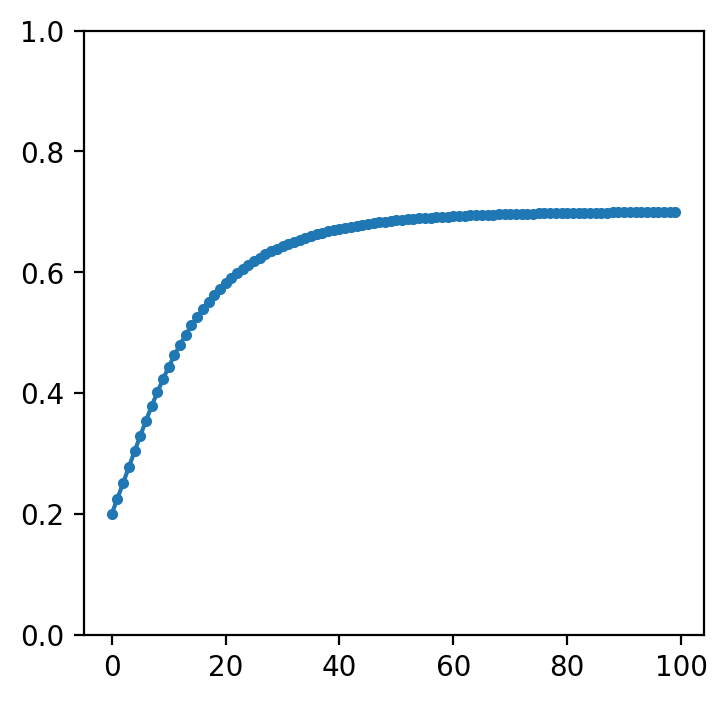
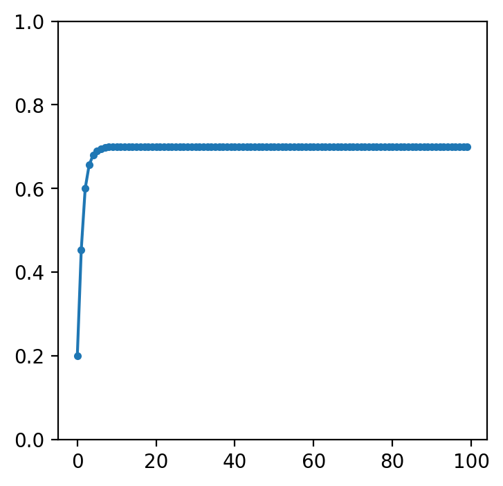
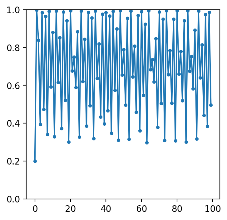
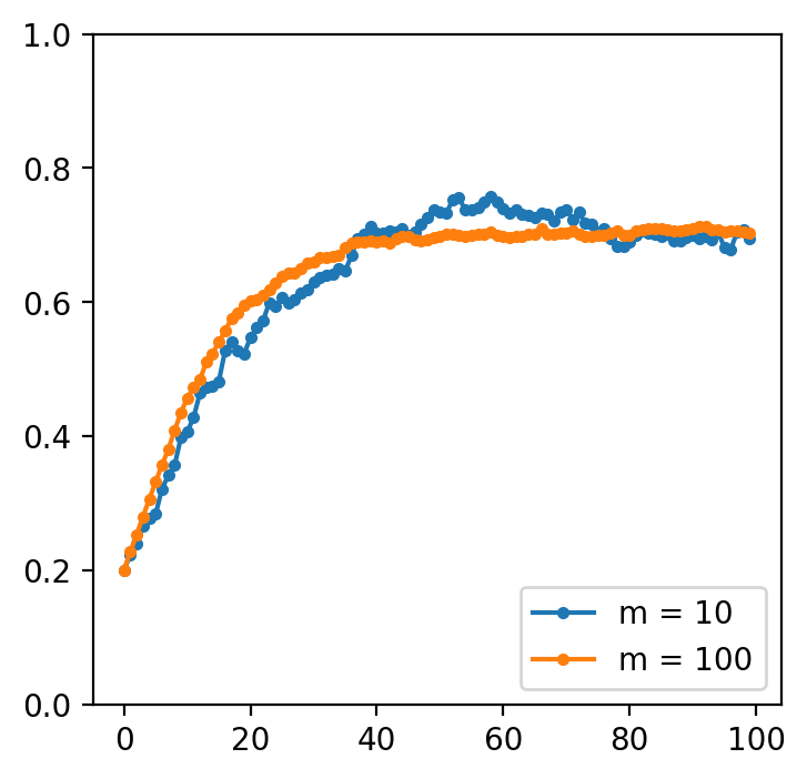
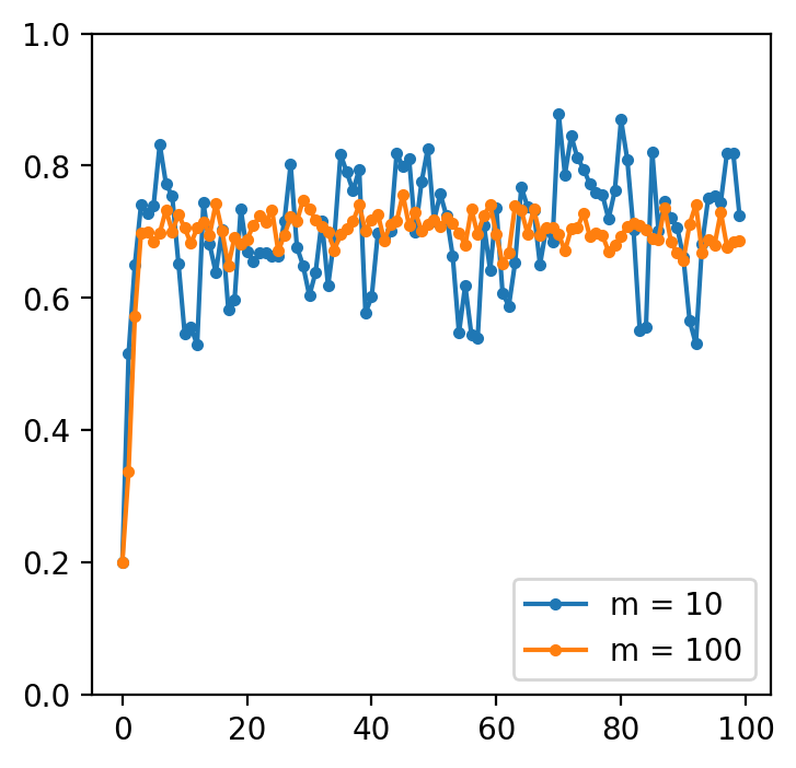
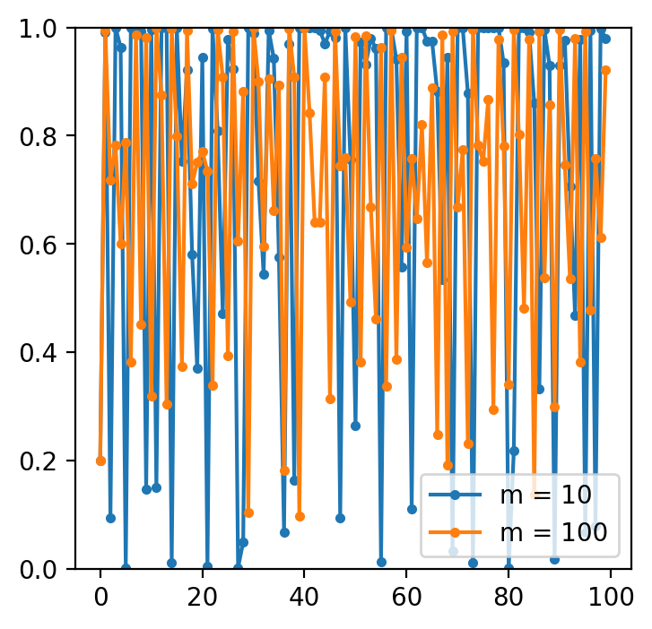
Figure 1: Here we plot the temporal behavior of ptsubscript𝑝𝑡p_{t} starting at p0=0.2subscript𝑝00.2p_{0}=0.2 for 100100100 rounds under various L𝐿L and η𝜂\eta, and noisy estimation of gradient of mean squared error with m𝑚m samples. The top row (figs. 1(c), 1(a) and 1(b)) present different combination of (L,η)𝐿𝜂(L,\eta), and bottom row (figs. 1(f), 1(d) and 1(e)) consider the gradient is estimated from m=10𝑚10m=10 and m=100𝑚100m=100 samples.

Now we simulate the one-dimensional dynamics in eq. 8 of one agent with different learning rate η𝜂\eta and collective influence L𝐿L.

We first define a location-scale distribution map. Let the feature x1,x2subscriptx1subscriptx2{\textnormal{x}}_{1},{\textnormal{x}}_{2} and noise x0subscriptx0{\textnormal{x}}_{0} are mutually independent Gaussian distribution with zero mean, and the variance are 𝔼[x12]=3𝔼delimited-[]superscriptsubscriptx123\mathbb{E}[{\textnormal{x}}_{1}^{2}]=3, 𝔼[x22]=7𝔼delimited-[]superscriptsubscriptx227\mathbb{E}[{\textnormal{x}}_{2}^{2}]=7, and 𝔼[x02]=1𝔼delimited-[]superscriptsubscriptx021\mathbb{E}[{\textnormal{x}}_{0}^{2}]=1. Finally, 𝜽0=𝟎superscript𝜽00{\bm{\theta}}^{0}={\bm{0}}. Therefore,

𝑨=𝔼[𝐱𝐱]=[3007], and 𝒃=𝑨𝜽0+𝔼[x0𝐱]=[00].formulae-sequence𝑨𝔼delimited-[]superscript𝐱𝐱topmatrix3007 and 𝒃𝑨superscript𝜽0𝔼delimited-[]subscriptx0𝐱matrix00{\bm{A}}=\mathbb{E}[{\mathbf{x}}{\mathbf{x}}^{\top}]=\begin{bmatrix}3&0\\ 0&7\end{bmatrix},\text{ and }{\bm{b}}={\bm{A}}{\bm{\theta}}^{0}+\mathbb{E}[{\textnormal{x}}_{0}{\mathbf{x}}]=\begin{bmatrix}0\\ 0\end{bmatrix}.

Given learning rate η>0𝜂0\eta>0, and collective influence L𝐿L, we have α(L)=20η(1+L)𝛼𝐿20𝜂1𝐿\alpha(L)=20\eta(1+L), and the performative stable point β(L)=0.7𝛽𝐿0.7\beta(L)=0.7.

The top row of fig. 1 shows the temporal behavior of ptsubscript𝑝𝑡p_{t} under different (L,η)𝐿𝜂(L,\eta). The bottom row in fig. 1 demonstrates our (convergent and chaotic) results are robust even when the value of gradient is noisy. Specifically, we consider at each round t𝑡t, instead of g1i(𝜽t)g2i(𝜽t)=2(1+L)(1,1)𝑨𝜽t2(1,1)𝒃superscriptsubscript𝑔1𝑖subscript𝜽𝑡superscriptsubscript𝑔2𝑖subscript𝜽𝑡21𝐿11𝑨subscript𝜽𝑡211𝒃g_{1}^{i}({\vec{\bm{\theta}}}_{t})-g_{2}^{i}({\vec{\bm{\theta}}}_{t})=2(1+L)(1,-1){\bm{A}}{\bm{\theta}}_{t}-2(1,-1){\bm{b}}, the agent replace 𝑨𝑨{\bm{A}} and 𝒃𝒃{\bm{b}} with empirical moments on m𝑚m samples. This process can be seen as a stochastic exponentiated gradient descent which uses a stochastic estimation of the gradient.

We can see chaotic behavior happens in fig. 1(c) with L=14𝐿14L=14 and η=0.05𝜂0.05\eta=0.05, and such behavior persists in fig. 1(f) when the evaluations of gradient are noisy. On the other hand, when the learning rate is small enough (figs. 1(a) and 1(b)) the dynamics converge to the performative stable point 0.70.70.7. Furthermore, in figs. 1(d) and 1(e) the dynamics converge even with noisy estimation of gradient.

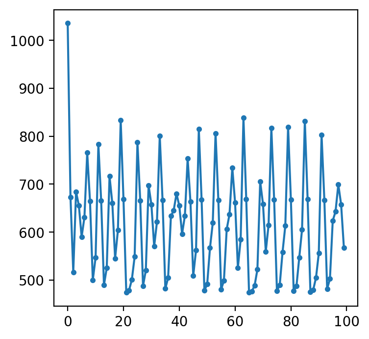
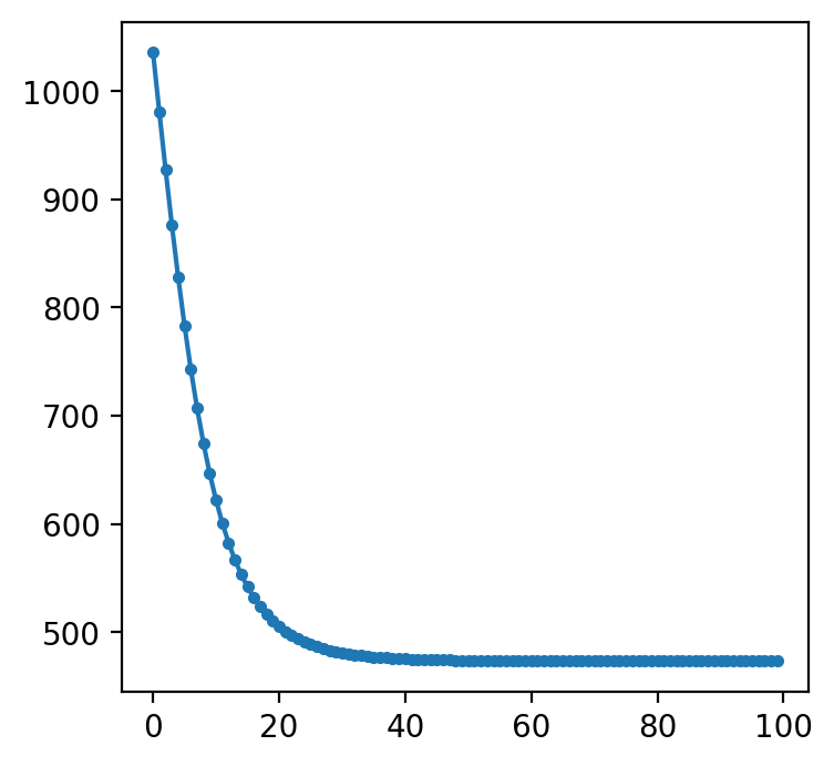
Finally, fig. 2 shows the temporal behavior of the loss. Under the same setting as fig. 1(c), fig. 2(b) shows not only the temporal behavior ptsubscript𝑝𝑡p_{t} is chaotic, but also the mean squared loss. On the other hand, under the same setting as fig. 1(a), fig. 2(a) shows convergent behavior of loss.
Refer to caption
(a) (14,0.001)140.001(14,0.001) without noise
Refer to caption
(b) (14,0.05)140.05(14,0.05) without noise
Figure 2: The temporal behavior of the total cost for 100100100 rounds under various η𝜂\eta.

6 Conclusion

We introduce a framework of multi-agent performative prediction and investigate whether classical reinforcement learning algorithms can converge or behave chaotically depending on the collective influence of the agents model and learning rate. However, we view our example as only scratching the surface of the work of multi-agent performative predictions.

Our framework leads to several new theoretical problems. In particular, it would be interesting to understand whether this threshold is generic and if our results still hold on other reinforcement learning algorithms or other general multi-agent distribution maps. Our framework also provides a new viewpoint to several applications. One natural application is strategic classification. [15] In this context, our framework can be seen as strategic learners in strategic classification problem where both data and classifiers are strategic. However, the features also respond to the deployed models in conventional strategic classification, which is not captured in our multi-agent location-scale distribution map. It would be interesting to investigate our dynamics in the context of strategic prediction. Another application is pricing strategy/prediction, where multiple companies predict the demand function and set their prices.

Both our digital and real-world environments are increasingly under the influence of or ever more powerful and numerous ML systems. As these algorithms trigger actions that change the state of the system that produces their joint input data (e.g., AI-triggered ads shown to users affecting their behavior, or automated trading systems affecting stock prices, etc), they are effectively forming closed loop systems and can no longer be understood fully in isolation. As we show in this paper, even fairly simple and innocuous such settings can exhibit phase transitions going from optimal behavior to chaos. We believe such phenomena are worthy of a careful investigation and we hope that this paper sets out some useful building blocks by bringing together optimization/performance analysis with Lyapunov theory and chaos theory.

References

  • Andrade et al. [2021] Gabriel P Andrade, Rafael Frongillo, and Georgios Piliouras. Learning in matrix games can be arbitrarily complex. In Conference on Learning Theory (COLT), 2021.
  • Bailey & Piliouras [2018] James P. Bailey and Georgios Piliouras. Multiplicative weights update in zero-sum games. In ACM Confernce on Economics and Computation, pp.  321–338, 2018.
  • Balduzzi et al. [2020] David Balduzzi, Wojciech M. Czarnecki, Thomas W. Anthony, Ian M. Gemp, Edward Hughes, Joel Z. Leibo, Georgios Piliouras, and Thore Graepel. Smooth markets: A basic mechanism for organizing gradient-based learners. CoRR, abs/2001.04678, 2020. URL https://arxiv.org/abs/2001.04678.
  • Bartlett [1992] Peter L Bartlett. Learning with a slowly changing distribution. In Proceedings of the fifth annual workshop on Computational learning theory, pp.  243–252, 1992.
  • Bielawski et al. [2021] Jakub Bielawski, Thiparat Chotibut, Fryderyk Falniowski, Grzegorz Kosiorowski, Michał Misiurewicz, and Georgios Piliouras. Follow-the-regularized-leader routes to chaos in routing games. ICML, 2021.
  • Cheung [2018] Yun Kuen Cheung. Multiplicative weights updates with constant step-size in graphical constant-sum games. In NeurIPS 2018, pp.  3532–3542, 2018.
  • Cheung & Piliouras [2020] Yun Kuen Cheung and Georgios Piliouras. Chaos, extremism and optimism: Volume analysis of learning in games. In NeurIPS 2020, 2020.
  • Cheung & Tao [2020] Yun Kuen Cheung and Yixin Tao. Chaos of learning beyond zero-sum and coordination via game decompositions. In International Conference on Learning Representations, 2020.
  • Cheung et al. [2021] Yun Kuen Cheung, Stefanos Leonardos, and Georgios Piliouras. Learning in markets: Greed leads to chaos but following the price is right. In Zhi-Hua Zhou (ed.), Proceedings of the Thirtieth International Joint Conference on Artificial Intelligence, IJCAI 2021, Virtual Event / Montreal, Canada, 19-27 August 2021, pp.  111–117. ijcai.org, 2021. doi: 10.24963/ijcai.2021/16.
  • Chotibut et al. [2020] Thiparat Chotibut, Fryderyk Falniowski, Michał Misiurewicz, and Georgios Piliouras. The route to chaos in routing games: When is price of anarchy too optimistic? NeurIPS, 2020.
  • Cohen et al. [2017] Johanne Cohen, Amélie Héliou, and Panayotis Mertikopoulos. Learning with bandit feedback in potential games. In Proceedings of the 31st International Conference on Neural Information Processing Systems, pp.  6372–6381, 2017.
  • Drusvyatskiy & Xiao [2020] Dmitriy Drusvyatskiy and Lin Xiao. Stochastic optimization with decision-dependent distributions, 2020.
  • Flokas et al. [2020] Lampros Flokas, Emmanouil-Vasileios Vlatakis-Gkaragkounis, Thanasis Lianeas, Panayotis Mertikopoulos, and Georgios Piliouras. No-regret learning and mixed nash equilibria: They do not mix. In Conference on Neural Information Processing Systems (NeurIPS), 2020.
  • Giannou et al. [2021] Angeliki Giannou, Emmanouil-Vasileios Vlatakis-Gkaragkounis, and Panayotis Mertikopoulos. Survival of the strictest: Stable and unstable equilibria under regularized learning with partial information. COLT, 2021.
  • Hardt et al. [2016] Moritz Hardt, Nimrod Megiddo, Christos Papadimitriou, and Mary Wootters. Strategic classification. In Proceedings of the 2016 ACM conference on innovations in theoretical computer science, pp.  111–122, 2016.
  • Izzo et al. [2021] Zachary Izzo, Lexing Ying, and James Zou. How to learn when data reacts to your model: performative gradient descent. arXiv preprint arXiv:2102.07698, 2021.
  • Kivinen & Warmuth [1997] Jyrki Kivinen and Manfred K Warmuth. Exponentiated gradient versus gradient descent for linear predictors. information and computation, 132(1):1–63, 1997.
  • Kleinberg et al. [2009] Robert Kleinberg, Georgios Piliouras, and Éva Tardos. Multiplicative updates outperform generic no-regret learning in congestion games. In Proceedings of the forty-first annual ACM symposium on Theory of computing, pp.  533–542, 2009.
  • Kuh et al. [1990] Anthony Kuh, Thomas Petsche, and Ronald L Rivest. Learning time-varying concepts. In NIPS, pp.  183–189, 1990.
  • Leonardos et al. [2021] Stefanos Leonardos, Barnabé Monnot, Daniël Reijsbergen, Stratis Skoulakis, and Georgios Piliouras. Dynamical analysis of the EIP-1559 ethereum fee market. CoRR, abs/2102.10567, 2021. URL https://arxiv.org/abs/2102.10567.
  • Letcher [2021] Alistair Letcher. On the impossibility of global convergence in multi-loss optimization. In International Conference on Learning Representations, 2021.
  • Li & Yorke [1975] Tien-Yien Li and James A. Yorke. Period three implies chaos. The American Mathematical Monthly, 82(10):985–992, 1975. ISSN 00029890, 19300972. URL http://www.jstor.org/stable/2318254.
  • Li et al. [1982] Tien-Yien Li, Michał Misiurewicz, Giulio Pianigiani, and James A. Yorke. Odd chaos. Physics Letters A, 87(6):271–273, 1982. ISSN 0375-9601. doi: https://doi.org/10.1016/0375-9601(82)90692-2. URL https://www.sciencedirect.com/science/article/pii/0375960182906922.
  • Mendler-Dünner et al. [2020] Celestine Mendler-Dünner, Juan C Perdomo, Tijana Zrnic, and Moritz Hardt. Stochastic optimization for performative prediction. arXiv preprint arXiv:2006.06887, 2020.
  • Miller et al. [2021] John Miller, Juan C Perdomo, and Tijana Zrnic. Outside the echo chamber: Optimizing the performative risk. arXiv preprint arXiv:2102.08570, 2021.
  • Palaiopanos et al. [2017] Gerasimos Palaiopanos, Ioannis Panageas, and Georgios Piliouras. Multiplicative weights update with constant step-size in congestion games: Convergence, limit cycles and chaos. CoRR, abs/1703.01138, 2017. URL http://arxiv.org/abs/1703.01138.
  • Panageas et al. [2019] Ioannis Panageas, Georgios Piliouras, and Xiao Wang. Multiplicative weights updates as a distributed constrained optimization algorithm: Convergence to second-order stationary points almost always. In International Conference on Machine Learning, pp. 4961–4969. PMLR, 2019.
  • Perdomo et al. [2020] Juan Perdomo, Tijana Zrnic, Celestine Mendler-Dünner, and Moritz Hardt. Performative prediction. In International Conference on Machine Learning, pp. 7599–7609. PMLR, 2020.
  • Vadori et al. [2021] Nelson Vadori, Rahul Savani, Thomas Spooner, and Sumitra Ganesh. Consensus multiplicative weights update: Learning to learn using projector-based game signatures. arXiv preprint arXiv:2106.02615, 2021.

Appendix A Proofs and Details in Section 3

Proof of LABEL:prop:existence.

First under the mean squared loss function, each agent i𝑖i’s decoupled performative loss function (𝜽,𝜽i)superscript𝜽superscript𝜽𝑖\ell({\vec{\bm{\theta}}}^{\prime},{\bm{\theta}}^{i}) is convex in 𝜽isuperscript𝜽𝑖{\bm{\theta}}^{i}. Thus, for linear predictive model, we can apply the KKT conditions on LABEL:def:stable so that a collection of predictive models 𝜽Θn𝜽superscriptΘ𝑛{\vec{\bm{\theta}}}\in\Theta^{n} is performatively stable if and only if for all i[n]𝑖delimited-[]𝑛i\in[n], k[d]𝑘delimited-[]𝑑k\in[d] with θki>0subscriptsuperscript𝜃𝑖𝑘0\theta^{i}_{k}>0, θki(𝜽,𝜽i)θli(𝜽,𝜽i)subscriptsuperscript𝜃𝑖𝑘superscript𝜽superscript𝜽𝑖subscriptsuperscript𝜃𝑖𝑙superscript𝜽superscript𝜽𝑖\frac{\partial}{\partial\theta^{i}_{k}}\ell({\vec{\bm{\theta}}}^{\prime},{\bm{\theta}}^{i})\leq\frac{\partial}{\partial\theta^{i}_{l}}\ell({\vec{\bm{\theta}}}^{\prime},{\bm{\theta}}^{i}) for all l[d]𝑙delimited-[]𝑑l\in[d] where 𝜽=𝜽superscript𝜽𝜽{\vec{\bm{\theta}}}^{\prime}={\vec{\bm{\theta}}}. Therefore, with eq. 1, 𝜽superscript𝜽{\vec{\bm{\theta}}}^{*} is performative stable if

gki(𝜽)gli(𝜽)subscriptsuperscript𝑔𝑖𝑘superscript𝜽subscriptsuperscript𝑔𝑖𝑙superscript𝜽g^{i}_{k}({\vec{\bm{\theta}}}^{*})\leq g^{i}_{l}({\vec{\bm{\theta}}}^{*}) (9)

holds for all i[n]𝑖delimited-[]𝑛i\in[n] and k[d]𝑘delimited-[]𝑑k\in[d] with θki>0subscriptsuperscript𝜃𝑖𝑘0\theta^{i}_{k}>0.

With eq. 9, we now show that there exists a unique performative stable point 𝜽superscript𝜽{\vec{\bm{\theta}}}^{*} by proving that 1) ΦΦ\Phi in eq. 2 is strictly convex, and 2) 𝜽superscript𝜽{\vec{\bm{\theta}}}^{*} is a minimizer of ΦΦ\Phi. First, to show ΦΦ\Phi is strictly convex, it is sufficient to show the Hessian of ΦΦ\Phi positive definite. Because ΦΦ\Phi is a quadratic function on ΘnsuperscriptΘ𝑛\Theta^{n}, the Hessian of ΦΦ\Phi is a constant matrix in nd×ndsuperscript𝑛𝑑𝑛𝑑\mathbb{R}^{nd\times nd} By the partial derivative of eq. 2, for all i,j[n]𝑖𝑗delimited-[]𝑛i,j\in[n] and k,l[d]𝑘𝑙delimited-[]𝑑k,l\in[d], we have (2Φ)ik,jl=2θkiθljΦ=2λiλjAk,lsubscriptsuperscript2Φ𝑖𝑘𝑗𝑙superscript2subscriptsuperscript𝜃𝑖𝑘subscriptsuperscript𝜃𝑗𝑙Φ2subscript𝜆𝑖subscript𝜆𝑗subscript𝐴𝑘𝑙(\nabla^{2}\Phi)_{ik,jl}=\frac{\partial^{2}}{\partial\theta^{i}_{k}\partial\theta^{j}_{l}}\Phi=2\lambda_{i}\lambda_{j}A_{k,l} if ij𝑖𝑗i\neq j and (2Φ)ik,il=2λi(λi+1)Ak,lsubscriptsuperscript2Φ𝑖𝑘𝑖𝑙2subscript𝜆𝑖subscript𝜆𝑖1subscript𝐴𝑘𝑙(\nabla^{2}\Phi)_{ik,il}=2\lambda_{i}(\lambda_{i}+1)A_{k,l}. Let 𝑳n×n𝑳superscript𝑛𝑛{\bm{L}}\in\mathbb{R}^{n\times n} with Lij=2λiλjsubscript𝐿𝑖𝑗2subscript𝜆𝑖subscript𝜆𝑗L_{ij}=2\lambda_{i}\lambda_{j} if ij𝑖𝑗i\neq j and 2λi(1+λi)2subscript𝜆𝑖1subscript𝜆𝑖2\lambda_{i}(1+\lambda_{i}) which is positive definite because λi>0subscript𝜆𝑖0\lambda_{i}>0 for all i[n]𝑖delimited-[]𝑛i\in[n]. Then, the Hessian of ΦΦ\Phi is the Kronecker product of 𝑳𝑳{\bm{L}} and 𝑨𝑨{\bm{A}},

2Φ=(2λ1(1+λ1)𝑨2λ1λn𝑨2λnλ1𝑨2λn(1+λn)𝑨)=𝑳𝑨.superscript2Φmatrix2subscript𝜆11subscript𝜆1𝑨2subscript𝜆1subscript𝜆𝑛𝑨2subscript𝜆𝑛subscript𝜆1𝑨2subscript𝜆𝑛1subscript𝜆𝑛𝑨tensor-product𝑳𝑨\nabla^{2}\Phi=\begin{pmatrix}2\lambda_{1}(1+\lambda_{1}){\bm{A}}&\dots&2\lambda_{1}\lambda_{n}{\bm{A}}\\ \vdots&\ddots&\vdots\\ 2\lambda_{n}\lambda_{1}{\bm{A}}&\dots&2\lambda_{n}(1+\lambda_{n}){\bm{A}}\end{pmatrix}={\bm{L}}\otimes{\bm{A}}.

Because 𝑳𝑳{\bm{L}} and 𝑨𝑨{\bm{A}} are both positive definite, the Hessian is also positive definite. Therefore, ΦΦ\Phi is strictly convex, and there exist a unique minimum of ΦΦ\Phi in the compact set ΘnsuperscriptΘ𝑛\Theta^{n}. Now we show 𝜽superscript𝜽{\vec{\bm{\theta}}}^{*} is performative stable if and only if 𝜽superscript𝜽{\vec{\bm{\theta}}}^{*} is a minimizer of ΦΦ\Phi. By the first order condition and the partial derivative of eq. 2, the minimum of eq. 2 at 𝜽superscript𝜽{\vec{\bm{\theta}}}^{*} if and only if gki(𝜽)gli(𝜽)subscriptsuperscript𝑔𝑖𝑘superscript𝜽subscriptsuperscript𝑔𝑖𝑙superscript𝜽g^{i}_{k}({\vec{\bm{\theta}}}^{*})\leq g^{i}_{l}({\vec{\bm{\theta}}}^{*}) for all i[n]𝑖delimited-[]𝑛i\in[n] k,l[d]𝑘𝑙delimited-[]𝑑k,l\in[d] with (θ)ki>0subscriptsuperscriptsuperscript𝜃𝑖𝑘0(\theta^{*})^{i}_{k}>0. Therefore, 𝜽superscript𝜽{\vec{\bm{\theta}}}^{*} is the minimum of ΦΦ\Phi if and only if 𝜽superscript𝜽{\vec{\bm{\theta}}}^{*} is a performative stable point. ∎

Proof of LABEL:prop:stable2optimal.

Given a profile of models 𝜽𝜽{\vec{\bm{\theta}}}, the total cost is

i(𝜽,(𝜽)i)=subscript𝑖𝜽superscript𝜽𝑖absent\displaystyle\sum_{i}\ell({\vec{\bm{\theta}}},({\bm{\theta}})^{i})= i𝔼(𝐱,y)𝒟(𝜽)[(y𝜽i𝐱)2]subscript𝑖subscript𝔼similar-to𝐱y𝒟𝜽delimited-[]superscriptysuperscript𝜽𝑖𝐱2\displaystyle\sum_{i}\mathbb{E}_{({\mathbf{x}},{\textnormal{y}})\sim\mathcal{D}({\vec{\bm{\theta}}})}[({\textnormal{y}}-{\bm{\theta}}^{i}\cdot{\mathbf{x}})^{2}]
=\displaystyle= i𝔼[(𝐱,𝜽0jλj𝜽j𝜽i+x0)2]subscript𝑖𝔼delimited-[]superscript𝐱superscript𝜽0subscript𝑗subscript𝜆𝑗superscript𝜽𝑗superscript𝜽𝑖subscript𝑥02\displaystyle\sum_{i}\mathbb{E}\left[\left(\left\langle{\mathbf{x}},{\bm{\theta}}^{0}-\sum_{j}\lambda_{j}{\bm{\theta}}^{j}-{\bm{\theta}}^{i}\right\rangle+x_{0}\right)^{2}\right]

which is a convex function on 𝜽Θn𝜽superscriptΘ𝑛{\vec{\bm{\theta}}}\in\Theta^{n}. Additionally,

θkiı(𝜽,𝜽ı)=(1+λi)gki(𝜽,𝜽)+ı[n]:ıiλigki(𝜽,𝜽)=(1+nλi)gki(𝜽,𝜽)subscriptsuperscript𝜃𝑖𝑘subscriptitalic-ı𝜽superscript𝜽italic-ı1subscript𝜆𝑖subscriptsuperscript𝑔𝑖𝑘𝜽𝜽subscript:italic-ıdelimited-[]𝑛italic-ı𝑖subscript𝜆𝑖subscriptsuperscript𝑔𝑖𝑘𝜽𝜽1𝑛subscript𝜆𝑖subscriptsuperscript𝑔𝑖𝑘𝜽𝜽\frac{\partial}{\partial\theta^{i}_{k}}\sum_{\imath}\ell({\vec{\bm{\theta}}},{\bm{\theta}}^{\imath})=(1+\lambda_{i})g^{i}_{k}({\vec{\bm{\theta}}},{\vec{\bm{\theta}}})+\sum_{\imath\in[n]:\imath\neq i}\lambda_{i}g^{i}_{k}({\vec{\bm{\theta}}},{\vec{\bm{\theta}}})=(1+n\lambda_{i})g^{i}_{k}({\vec{\bm{\theta}}},{\vec{\bm{\theta}}})

which is the gradient of decoupled performative loss scaled by (1+nλi)1𝑛subscript𝜆𝑖(1+n\lambda_{i}). Thus, we can apply the KKT conditions and the minimum happens if and only if eq. 9 holds. ∎

Appendix B Proof and Details for Theorem LABEL:thm:converge_conti

Proof of LABEL:lem:potential_conti.

By chain rule,

ddtΦ(ϑ(t))=i[n],k[d]θki(ϑ(t))ddtϑ(t),𝑑𝑑𝑡Φbold-italic-ϑ𝑡subscriptformulae-sequence𝑖delimited-[]𝑛𝑘delimited-[]𝑑subscriptsuperscript𝜃𝑖𝑘bold-italic-ϑ𝑡𝑑𝑑𝑡bold-italic-ϑ𝑡\frac{d}{dt}\Phi(\vec{\bm{\vartheta}}(t))=\sum_{i\in[n],k\in[d]}\frac{\partial}{\partial\theta^{i}_{k}}(\vec{\bm{\vartheta}}(t))\cdot\frac{d}{dt}\vec{\bm{\vartheta}}(t), (10)

so the time derivative of the potential function is zero if the dynamics is at a fixed point of eq. 6.

Now we compute a closed form of the time derivative and show the derivative is zero only if the dynamics is at a fixed point of eq. 6. Here we omit the input t𝑡t to simplify the notation.

ddtΦ(ϑ(t))=𝑑𝑑𝑡Φbold-italic-ϑ𝑡absent\displaystyle\frac{d}{dt}\Phi(\vec{\bm{\vartheta}}(t))= i,kθki(ϑ(t))ηi𝜼1ϑki(t)(lϑli(t)gli(ϑ(t))gki(ϑ(t)))subscript𝑖𝑘subscriptsuperscript𝜃𝑖𝑘bold-italic-ϑ𝑡subscript𝜂𝑖subscriptnorm𝜼1subscriptsuperscriptitalic-ϑ𝑖𝑘𝑡subscript𝑙subscriptsuperscriptitalic-ϑ𝑖𝑙𝑡subscriptsuperscript𝑔𝑖𝑙bold-italic-ϑ𝑡subscriptsuperscript𝑔𝑖𝑘bold-italic-ϑ𝑡\displaystyle\sum_{i,k}\frac{\partial}{\partial\theta^{i}_{k}}(\vec{\bm{\vartheta}}(t))\cdot\frac{\eta_{i}}{\|\bm{\eta}\|_{1}}\vartheta^{i}_{k}(t)(\sum_{l}\vartheta^{i}_{l}(t)g^{i}_{l}(\vec{\bm{\vartheta}}(t))-g^{i}_{k}(\vec{\bm{\vartheta}}(t))) (by eqs. 6 and 10)
=\displaystyle= 1𝜼1iλiηi(k(gki)ϑki(lϑligligki))1subscriptnorm𝜼1subscript𝑖subscript𝜆𝑖subscript𝜂𝑖subscript𝑘subscriptsuperscript𝑔𝑖𝑘subscriptsuperscriptitalic-ϑ𝑖𝑘subscript𝑙subscriptsuperscriptitalic-ϑ𝑖𝑙subscriptsuperscript𝑔𝑖𝑙subscriptsuperscript𝑔𝑖𝑘\displaystyle\frac{1}{\|\bm{\eta}\|_{1}}\sum_{i}\lambda_{i}\eta_{i}\left(\sum_{k}\left(g^{i}_{k}\right)\cdot\vartheta^{i}_{k}\left(\sum_{l}\vartheta^{i}_{l}g^{i}_{l}-g^{i}_{k}\right)\right) (by the partial derivative of eq. 2)
=\displaystyle= 12𝜼1iλiηik,l[d]ϑkiϑli(2gkigli2(gki)2)12subscriptnorm𝜼1subscript𝑖subscript𝜆𝑖subscript𝜂𝑖subscript𝑘𝑙delimited-[]𝑑subscriptsuperscriptitalic-ϑ𝑖𝑘subscriptsuperscriptitalic-ϑ𝑖𝑙2subscriptsuperscript𝑔𝑖𝑘subscriptsuperscript𝑔𝑖𝑙2superscriptsubscriptsuperscript𝑔𝑖𝑘2\displaystyle\frac{1}{2\|\bm{\eta}\|_{1}}\sum_{i}\lambda_{i}\eta_{i}\sum_{k,l\in[d]}\vartheta^{i}_{k}\vartheta^{i}_{l}(2g^{i}_{k}g^{i}_{l}-2(g^{i}_{k})^{2}) (because lϑli=1subscript𝑙subscriptsuperscriptitalic-ϑ𝑖𝑙1\sum_{l}\vartheta^{i}_{l}=1)
=\displaystyle= 12𝜼1iλiηik,l[d]ϑkiϑli(gkigli)212subscriptnorm𝜼1subscript𝑖subscript𝜆𝑖subscript𝜂𝑖subscript𝑘𝑙delimited-[]𝑑subscriptsuperscriptitalic-ϑ𝑖𝑘subscriptsuperscriptitalic-ϑ𝑖𝑙superscriptsubscriptsuperscript𝑔𝑖𝑘subscriptsuperscript𝑔𝑖𝑙2\displaystyle\frac{-1}{2\|\bm{\eta}\|_{1}}\sum_{i}\lambda_{i}\eta_{i}\sum_{k,l\in[d]}\vartheta^{i}_{k}\vartheta^{i}_{l}(g^{i}_{k}-g^{i}_{l})^{2}

Now we bound the time derivative.

2𝜼1(iλiηi)ddtΦ(ϑ(t))2subscriptnorm𝜼1subscript𝑖subscript𝜆𝑖subscript𝜂𝑖𝑑𝑑𝑡Φbold-italic-ϑ𝑡\displaystyle-2\|\bm{\eta}\|_{1}\left(\sum_{i}\lambda_{i}\eta_{i}\right)\frac{d}{dt}\Phi(\vec{\bm{\vartheta}}(t))
=\displaystyle= (i[n],k,l[d]λiηiϑkiϑli)(i[n],k,l[d]λiηiϑkiϑli(gkigli)2)subscriptformulae-sequence𝑖delimited-[]𝑛𝑘𝑙delimited-[]𝑑subscript𝜆𝑖subscript𝜂𝑖subscriptsuperscriptitalic-ϑ𝑖𝑘subscriptsuperscriptitalic-ϑ𝑖𝑙subscriptformulae-sequence𝑖delimited-[]𝑛𝑘𝑙delimited-[]𝑑subscript𝜆𝑖subscript𝜂𝑖subscriptsuperscriptitalic-ϑ𝑖𝑘subscriptsuperscriptitalic-ϑ𝑖𝑙superscriptsubscriptsuperscript𝑔𝑖𝑘subscriptsuperscript𝑔𝑖𝑙2\displaystyle\left(\sum_{i\in[n],k,l\in[d]}\lambda_{i}\eta_{i}\vartheta^{i}_{k}\vartheta^{i}_{l}\right)\left(\sum_{i\in[n],k,l\in[d]}\lambda_{i}\eta_{i}\vartheta^{i}_{k}\vartheta^{i}_{l}(g^{i}_{k}-g^{i}_{l})^{2}\right) (kϑki=lϑli=1subscript𝑘subscriptsuperscriptitalic-ϑ𝑖𝑘subscript𝑙subscriptsuperscriptitalic-ϑ𝑖𝑙1\sum_{k}\vartheta^{i}_{k}=\sum_{l}\vartheta^{i}_{l}=1)
\displaystyle\geq (i[n],k,l[d]λiηiϑkiϑli|gkigli|)2.superscriptsubscriptformulae-sequence𝑖delimited-[]𝑛𝑘𝑙delimited-[]𝑑subscript𝜆𝑖subscript𝜂𝑖subscriptsuperscriptitalic-ϑ𝑖𝑘subscriptsuperscriptitalic-ϑ𝑖𝑙subscriptsuperscript𝑔𝑖𝑘subscriptsuperscript𝑔𝑖𝑙2\displaystyle\left(\sum_{i\in[n],k,l\in[d]}\lambda_{i}\eta_{i}\vartheta^{i}_{k}\vartheta^{i}_{l}|g^{i}_{k}-g^{i}_{l}|\right)^{2}. (by Cauchy inequality)
\displaystyle\geq (i[n],k[d]λiηi|ϑkil[d]ϑli(gkigli)|)2superscriptsubscriptformulae-sequence𝑖delimited-[]𝑛𝑘delimited-[]𝑑subscript𝜆𝑖subscript𝜂𝑖subscriptsuperscriptitalic-ϑ𝑖𝑘subscript𝑙delimited-[]𝑑subscriptsuperscriptitalic-ϑ𝑖𝑙subscriptsuperscript𝑔𝑖𝑘subscriptsuperscript𝑔𝑖𝑙2\displaystyle\left(\sum_{i\in[n],k\in[d]}\lambda_{i}\eta_{i}\left|\vartheta^{i}_{k}\sum_{l\in[d]}\vartheta^{i}_{l}(g^{i}_{k}-g^{i}_{l})\right|\right)^{2} (by triangle inequality)

Therefore, ddtΦ(ϑ(t))=0𝑑𝑑𝑡Φbold-italic-ϑ𝑡0\frac{d}{dt}\Phi(\vec{\bm{\vartheta}}(t))=0 only if ϑki(gkil[d]ϑligli)=0subscriptsuperscriptitalic-ϑ𝑖𝑘subscriptsuperscript𝑔𝑖𝑘subscript𝑙delimited-[]𝑑subscriptsuperscriptitalic-ϑ𝑖𝑙subscriptsuperscript𝑔𝑖𝑙0\vartheta^{i}_{k}\left(g^{i}_{k}-\sum_{l\in[d]}\vartheta^{i}_{l}g^{i}_{l}\right)=0 for all i[n]𝑖delimited-[]𝑛i\in[n] and k[d]𝑘delimited-[]𝑑k\in[d] which is a fixed point of eq. 6.

We can further simplify the bound by 𝝃𝝃{\vec{\bm{\xi}}}. Because i,kλiηi|ϑki(lϑligligki)|(miniλiηi)i,k|ξki(ϑ)|=(miniλiηi)𝝃(ϑ)1subscript𝑖𝑘subscript𝜆𝑖subscript𝜂𝑖subscriptsuperscriptitalic-ϑ𝑖𝑘subscript𝑙subscriptsuperscriptitalic-ϑ𝑖𝑙subscriptsuperscript𝑔𝑖𝑙subscriptsuperscript𝑔𝑖𝑘subscript𝑖subscript𝜆𝑖subscript𝜂𝑖subscript𝑖𝑘subscriptsuperscript𝜉𝑖𝑘bold-italic-ϑsubscript𝑖subscript𝜆𝑖subscript𝜂𝑖subscriptnorm𝝃bold-italic-ϑ1\sum_{i,k}\lambda_{i}\eta_{i}|\vartheta^{i}_{k}(\sum_{l}\vartheta^{i}_{l}g^{i}_{l}-g^{i}_{k})|\geq\left(\min_{i}\lambda_{i}\eta_{i}\right)\sum_{i,k}|\xi^{i}_{k}({\vec{\bm{\vartheta}}})|=\left(\min_{i}\lambda_{i}\eta_{i}\right)\|{\vec{\bm{\xi}}}({\vec{\bm{\vartheta}}})\|_{1}, ddtΦ(ϑ(t))miniλiηi2iηiiλiηi𝝃(ϑ)12𝑑𝑑𝑡Φbold-italic-ϑ𝑡subscript𝑖subscript𝜆𝑖subscript𝜂𝑖2subscript𝑖subscript𝜂𝑖subscript𝑖subscript𝜆𝑖subscript𝜂𝑖superscriptsubscriptnorm𝝃bold-italic-ϑ12\frac{d}{dt}\Phi(\vec{\bm{\vartheta}}(t))\leq\frac{-\min_{i}\lambda_{i}\eta_{i}}{2\sum_{i}\eta_{i}\sum_{i}\lambda_{i}\eta_{i}}\|{\vec{\bm{\xi}}}({\vec{\bm{\vartheta}}})\|_{1}^{2}. ∎

Proof of LABEL:thm:converge_conti.

When the fixed points are isolated satisfying eq. 4, by LABEL:lem:potential_conti, the dynamics in eq. 6 converges to a fixed point of eq. 6, 𝜽Θnsuperscript𝜽superscriptΘ𝑛{\vec{\bm{\theta}}}^{*}\in\Theta^{n}. Because 𝜽superscript𝜽{\vec{\bm{\theta}}}^{*} is a fixed point, for all i[n],k[d]formulae-sequence𝑖delimited-[]𝑛𝑘delimited-[]𝑑i\in[n],k\in[d],

(θ)ki(g¯i(𝜽)gki(𝜽))=(θ)kil(θ)ligli(𝜽)gki(𝜽)=0subscriptsuperscriptsuperscript𝜃𝑖𝑘superscript¯𝑔𝑖superscript𝜽subscriptsuperscript𝑔𝑖𝑘superscript𝜽subscriptsuperscriptsuperscript𝜃𝑖𝑘subscript𝑙subscriptsuperscriptsuperscript𝜃𝑖𝑙subscriptsuperscript𝑔𝑖𝑙superscript𝜽subscriptsuperscript𝑔𝑖𝑘superscript𝜽0(\theta^{*})^{i}_{k}\left(\bar{g}^{i}({\vec{\bm{\theta}}}^{*})-g^{i}_{k}({\vec{\bm{\theta}}}^{*})\right)=(\theta^{*})^{i}_{k}\sum_{l}(\theta^{*})^{i}_{l}g^{i}_{l}({\vec{\bm{\theta}}}^{*})-g^{i}_{k}({\vec{\bm{\theta}}}^{*})=0

By LABEL:prop:existence, the fixed point condition implies each coordinate of the gradient of loss in the support are identical, gki(𝜽)=g¯i(𝜽)subscriptsuperscript𝑔𝑖𝑘superscript𝜽superscript¯𝑔𝑖superscript𝜽g^{i}_{k}({\vec{\bm{\theta}}}^{*})=\bar{g}^{i}({\vec{\bm{\theta}}}^{*}) for all i𝑖i and kSi𝑘subscript𝑆𝑖k\in S_{i}. Thus, if the fixed point 𝜽superscript𝜽{\vec{\bm{\theta}}}^{*} is not performative stable, there exists ıitalic-ı\imath and κ𝜅\kappa with (θ)κı=0subscriptsuperscriptsuperscript𝜃italic-ı𝜅0(\theta^{*})^{\imath}_{\kappa}=0 so that gκı(𝜽)<g¯ı(𝜽)subscriptsuperscript𝑔italic-ı𝜅superscript𝜽superscript¯𝑔italic-ısuperscript𝜽g^{\imath}_{\kappa}({\vec{\bm{\theta}}}^{*})<\bar{g}^{\imath}({\vec{\bm{\theta}}}^{*}). Furthermore, exp(ηıgκı(𝜽))>l(θ)lıexp(ηıglı(𝜽))subscript𝜂italic-ısubscriptsuperscript𝑔italic-ı𝜅superscript𝜽subscript𝑙subscriptsuperscriptsuperscript𝜃italic-ı𝑙subscript𝜂italic-ısubscriptsuperscript𝑔italic-ı𝑙superscript𝜽\exp(-\eta_{\imath}g^{\imath}_{\kappa}({\vec{\bm{\theta}}}^{*}))>\sum_{l}(\theta^{*})^{\imath}_{l}\exp(-\eta_{\imath}g^{\imath}_{l}({\vec{\bm{\theta}}}^{*})). We can pick a small enough ϵ>0italic-ϵ0\epsilon>0 and define

Uϵ:={𝜽:exp(ηıgκı)>lθlıexp(ηıglı)+ϵ}assignsubscript𝑈italic-ϵconditional-set𝜽subscript𝜂italic-ısubscriptsuperscript𝑔italic-ı𝜅subscript𝑙subscriptsuperscript𝜃italic-ı𝑙subscript𝜂italic-ısubscriptsuperscript𝑔italic-ı𝑙italic-ϵU_{\epsilon}:=\{{\vec{\bm{\theta}}}:\exp(-\eta_{\imath}g^{\imath}_{\kappa})>\sum_{l}\theta^{\imath}_{l}\exp(-\eta_{\imath}g^{\imath}_{l})+\epsilon\} (11)

which contains 𝜽superscript𝜽{\vec{\bm{\theta}}}^{*} and is an open set because 𝒈𝒈\vec{{\bm{g}}} and the exponential function are continuous. Since ϑ(t)bold-italic-ϑ𝑡\vec{\bm{\vartheta}}(t) converges to 𝜽superscript𝜽{\vec{\bm{\theta}}}^{*} as t𝑡t\to\infty, there exists a time tϵsubscript𝑡italic-ϵt_{\epsilon} so that for all ttϵ𝑡subscript𝑡italic-ϵt\geq t_{\epsilon}, ϑ(t)Uϵbold-italic-ϑ𝑡subscript𝑈italic-ϵ\vec{\bm{\vartheta}}(t)\in U_{\epsilon}. However, if ϑ(t)Uϵbold-italic-ϑ𝑡subscript𝑈italic-ϵ\vec{\bm{\vartheta}}(t)\in U_{\epsilon} and ϑ(t)bold-italic-ϑ𝑡\vec{\bm{\vartheta}}(t) is an interior point, we get ddtϑki(t)>0𝑑𝑑𝑡subscriptsuperscriptitalic-ϑ𝑖𝑘𝑡0\frac{d}{dt}\vartheta^{i}_{k}(t)>0 by eqs. 6 and 11. Therefore, ϑki(t)subscriptsuperscriptitalic-ϑ𝑖𝑘𝑡\vartheta^{i}_{k}(t) is positive and increasing for ttϵ𝑡subscript𝑡italic-ϵt\geq t_{\epsilon}. We reached a contradiction because ϑki(t)(θ)ki=0subscriptsuperscriptitalic-ϑ𝑖𝑘𝑡subscriptsuperscriptsuperscript𝜃𝑖𝑘0\vartheta^{i}_{k}(t)\to(\theta^{*})^{i}_{k}=0. Therefore, 𝜽superscript𝜽{\vec{\bm{\theta}}}^{*} is a performative stable point. ∎

Appendix C Proof ans Details for Theorem LABEL:thm:converge_const

To prove LABEL:thm:converge_const, show the dynamic eq. 3 can be approximated by eq. 6 and the error vanishes as ηsubscript𝜂\eta_{*} decreases. Thus, we can show the dynamic can hit an arbitrary neighborhood of the performative stable point. We further use ΦΦ\Phi to show the dynamic will stay in the neighborhood. Below we state two ancillary lemmas to control the error of our approximation.

We define an error vector 𝒆(𝜽)n×d𝒆𝜽superscript𝑛𝑑\vec{{\bm{e}}}({\vec{\bm{\theta}}})\in\mathbb{R}^{n\times d} between eqs. 3 and 6 so that

ηi2eki(𝜽):=θkiexp(ηi(g¯igki))lθliexp(ηi(g¯igli))θkiηiξkiassignsuperscriptsubscript𝜂𝑖2subscriptsuperscript𝑒𝑖𝑘𝜽subscriptsuperscript𝜃𝑖𝑘subscript𝜂𝑖superscript¯𝑔𝑖subscriptsuperscript𝑔𝑖𝑘subscript𝑙subscriptsuperscript𝜃𝑖𝑙subscript𝜂𝑖superscript¯𝑔𝑖subscriptsuperscript𝑔𝑖𝑙subscriptsuperscript𝜃𝑖𝑘subscript𝜂𝑖subscriptsuperscript𝜉𝑖𝑘\eta_{i}^{2}e^{i}_{k}({\vec{\bm{\theta}}}):=\frac{\theta^{i}_{k}\exp(\eta_{i}(\bar{g}^{i}-g^{i}_{k}))}{\sum_{l}\theta^{i}_{l}\exp(\eta_{i}(\bar{g}^{i}-g^{i}_{l}))}-\theta^{i}_{k}-\eta_{i}\xi^{i}_{k}

We omit the input 𝜽𝜽{\vec{\bm{\theta}}} of 𝒆𝒆\vec{{\bm{e}}} and 𝒆t:=𝒆(𝜽t)assignsubscript𝒆𝑡𝒆subscript𝜽𝑡\vec{{\bm{e}}}_{t}:=\vec{{\bm{e}}}({\vec{\bm{\theta}}}_{t}) when there is no ambiguity. We show if the the error vector is small, ΦΦ\Phi is decreasing in dynamics eq. 3.

Claim C.1 (name = Approximated potential, label = lem:potential_dis).

There exist C4subscript𝐶4C_{4}, so that for all t𝑡t and 𝛉0Θnsubscript𝛉0superscriptΘ𝑛{\vec{\bm{\theta}}}_{0}\in\Theta^{n}, the difference of eq. 2 on eq. 3 satisfies

Φ(𝜽t+1)Φ(𝜽t)miniλi2ηi22iλiηi𝝃t12+maxiλiηi2maxi,k,𝜽|gki(𝜽)|𝒆t1+d2C4𝜽t+1𝜽t12.Φsubscript𝜽𝑡1Φsubscript𝜽𝑡subscript𝑖superscriptsubscript𝜆𝑖2superscriptsubscript𝜂𝑖22subscript𝑖subscript𝜆𝑖subscript𝜂𝑖superscriptsubscriptnormsubscript𝝃𝑡12subscript𝑖subscript𝜆𝑖superscriptsubscript𝜂𝑖2subscript𝑖𝑘𝜽subscriptsuperscript𝑔𝑖𝑘𝜽subscriptnormsubscript𝒆𝑡1superscript𝑑2subscript𝐶4subscriptsuperscriptnormsubscript𝜽𝑡1subscript𝜽𝑡21\Phi({\vec{\bm{\theta}}}_{t+1})-\Phi({\vec{\bm{\theta}}}_{t})\leq\frac{-\min_{i}\lambda_{i}^{2}\eta_{i}^{2}}{2\sum_{i}\lambda_{i}\eta_{i}}\|{\vec{\bm{\xi}}}_{t}\|_{1}^{2}+\max_{i}\lambda_{i}\eta_{i}^{2}\max_{i,k,{\vec{\bm{\theta}}}}|g^{i}_{k}({\vec{\bm{\theta}}})|\cdot\|\vec{{\bm{e}}}_{t}\|_{1}+d^{2}C_{4}\left\|{\vec{\bm{\theta}}}_{t+1}-{\vec{\bm{\theta}}}_{t}\right\|^{2}_{1}.
Claim C.2 (label = lem:err_const).

If maxiηisubscript𝑖subscript𝜂𝑖\max_{i}\eta_{i} is small enough and satisfies eq. 12, there exists a constant C𝐶C so that

|eki(𝜽)|C for all i[n],k[d], and 𝜽Θn.formulae-sequencesubscriptsuperscript𝑒𝑖𝑘𝜽𝐶 for all 𝑖delimited-[]𝑛formulae-sequence𝑘delimited-[]𝑑 and 𝜽superscriptΘ𝑛|e^{i}_{k}({\vec{\bm{\theta}}})|\leq C\text{ for all }i\in[n],k\in[d],\text{ and }{\vec{\bm{\theta}}}\in\Theta^{n}.

The proofs of these two claims are based on first order approximation.

Proof of LABEL:lem:potential_dis.

By the partial derivative of eq. 2, we have 2θkiθljΦ(𝜽)=2λiλjAl,ksuperscript2subscriptsuperscript𝜃𝑖𝑘subscriptsuperscript𝜃𝑗𝑙Φ𝜽2subscript𝜆𝑖subscript𝜆𝑗subscript𝐴𝑙𝑘\frac{\partial^{2}}{\partial\theta^{i}_{k}\partial\theta^{j}_{l}}\Phi({\vec{\bm{\theta}}})=2\lambda_{i}\lambda_{j}A_{l,k} if ij𝑖𝑗i\neq j and 2θkiθliΦ(𝜽)=2λi(1+λi)Al,ksuperscript2subscriptsuperscript𝜃𝑖𝑘subscriptsuperscript𝜃𝑖𝑙Φ𝜽2subscript𝜆𝑖1subscript𝜆𝑖subscript𝐴𝑙𝑘\frac{\partial^{2}}{\partial\theta^{i}_{k}\partial\theta^{i}_{l}}\Phi({\vec{\bm{\theta}}})=2\lambda_{i}(1+\lambda_{i})A_{l,k}. Thus, the second order partial derivatives of ΦΦ\Phi can bounded by the twice of C4:=maxıλı(λı+1)maxk,lAk,lassignsubscript𝐶4subscriptitalic-ısubscript𝜆italic-ısubscript𝜆italic-ı1subscript𝑘𝑙subscript𝐴𝑘𝑙C_{4}:=\max_{\imath}\lambda_{\imath}(\lambda_{\imath}+1)\max_{k,l}A_{k,l}. By Taylor’s expansion, we have

Φ(𝜽t+1)Φ(𝜽t)Φsubscript𝜽𝑡1Φsubscript𝜽𝑡\displaystyle\Phi({\vec{\bm{\theta}}}_{t+1})-\Phi({\vec{\bm{\theta}}}_{t})
\displaystyle\leq Φ(𝜽t)(𝜽t+1𝜽t)+d22C42𝜽(t+1)𝜽(t)22Φsubscript𝜽𝑡subscript𝜽𝑡1subscript𝜽𝑡superscript𝑑22subscript𝐶42subscriptsuperscriptnorm𝜽𝑡1𝜽𝑡22\displaystyle\nabla\Phi({\vec{\bm{\theta}}}_{t})\cdot\left({\vec{\bm{\theta}}}_{t+1}-{\vec{\bm{\theta}}}_{t}\right)+\frac{d^{2}2C_{4}}{2}\left\|{\vec{\bm{\theta}}}(t+1)-{\vec{\bm{\theta}}}(t)\right\|^{2}_{2}
\displaystyle\leq i[n],k[d]λigki(𝜽t)(ηiξki(𝜽t)+ηi2eki(𝜽t))+d2C4𝜽(t+1)𝜽(t)12subscriptformulae-sequence𝑖delimited-[]𝑛𝑘delimited-[]𝑑subscript𝜆𝑖subscriptsuperscript𝑔𝑖𝑘subscript𝜽𝑡subscript𝜂𝑖subscriptsuperscript𝜉𝑖𝑘subscript𝜽𝑡superscriptsubscript𝜂𝑖2subscriptsuperscript𝑒𝑖𝑘subscript𝜽𝑡superscript𝑑2subscript𝐶4subscriptsuperscriptnorm𝜽𝑡1𝜽𝑡21\displaystyle\sum_{i\in[n],k\in[d]}\lambda_{i}g^{i}_{k}({\vec{\bm{\theta}}}_{t})(\eta_{i}\xi^{i}_{k}({\vec{\bm{\theta}}}_{t})+\eta_{i}^{2}e^{i}_{k}({\vec{\bm{\theta}}}_{t}))+d^{2}C_{4}\left\|{\vec{\bm{\theta}}}(t+1)-{\vec{\bm{\theta}}}(t)\right\|^{2}_{1} (by the partial derivative of eq. 2)
=\displaystyle= i[n],k[d]λiηigt,kiξt,ki+λiηi2gt,kiet,ki+d2C4𝜽t+1𝜽t12subscriptformulae-sequence𝑖delimited-[]𝑛𝑘delimited-[]𝑑subscript𝜆𝑖subscript𝜂𝑖subscriptsuperscript𝑔𝑖𝑡𝑘subscriptsuperscript𝜉𝑖𝑡𝑘subscript𝜆𝑖superscriptsubscript𝜂𝑖2subscriptsuperscript𝑔𝑖𝑡𝑘subscriptsuperscript𝑒𝑖𝑡𝑘superscript𝑑2subscript𝐶4subscriptsuperscriptnormsubscript𝜽𝑡1subscript𝜽𝑡21\displaystyle\sum_{i\in[n],k\in[d]}\lambda_{i}\eta_{i}g^{i}_{t,k}\xi^{i}_{t,k}+\lambda_{i}\eta_{i}^{2}g^{i}_{t,k}e^{i}_{t,k}+d^{2}C_{4}\left\|{\vec{\bm{\theta}}}_{t+1}-{\vec{\bm{\theta}}}_{t}\right\|^{2}_{1}
\displaystyle\leq 12iλiηi(i,kλiηi|ξt,ki|)2+i[n],k[d]λiηi2gt,kiet,ki+d2C4𝜽t+1𝜽t1212subscript𝑖subscript𝜆𝑖subscript𝜂𝑖superscriptsubscript𝑖𝑘subscript𝜆𝑖subscript𝜂𝑖subscriptsuperscript𝜉𝑖𝑡𝑘2subscriptformulae-sequence𝑖delimited-[]𝑛𝑘delimited-[]𝑑subscript𝜆𝑖superscriptsubscript𝜂𝑖2subscriptsuperscript𝑔𝑖𝑡𝑘subscriptsuperscript𝑒𝑖𝑡𝑘superscript𝑑2subscript𝐶4subscriptsuperscriptnormsubscript𝜽𝑡1subscript𝜽𝑡21\displaystyle\frac{-1}{2\sum_{i}\lambda_{i}\eta_{i}}\left(\sum_{i,k}\lambda_{i}\eta_{i}|\xi^{i}_{t,k}|\right)^{2}+\sum_{i\in[n],k\in[d]}\lambda_{i}\eta_{i}^{2}g^{i}_{t,k}e^{i}_{t,k}+d^{2}C_{4}\left\|{\vec{\bm{\theta}}}_{t+1}-{\vec{\bm{\theta}}}_{t}\right\|^{2}_{1} (by LABEL:lem:potential_conti)

Therefore, we have

Φ(𝜽t+1)Φ(𝜽t)miniλi2ηi22iλiηi𝝃t12+maxiλiηi2maxi,k,𝜽|gki(𝜽)|𝒆t1+d2C4𝜽t+1𝜽t12Φsubscript𝜽𝑡1Φsubscript𝜽𝑡subscript𝑖superscriptsubscript𝜆𝑖2superscriptsubscript𝜂𝑖22subscript𝑖subscript𝜆𝑖subscript𝜂𝑖superscriptsubscriptnormsubscript𝝃𝑡12subscript𝑖subscript𝜆𝑖superscriptsubscript𝜂𝑖2subscript𝑖𝑘𝜽subscriptsuperscript𝑔𝑖𝑘𝜽subscriptnormsubscript𝒆𝑡1superscript𝑑2subscript𝐶4subscriptsuperscriptnormsubscript𝜽𝑡1subscript𝜽𝑡21\Phi({\vec{\bm{\theta}}}_{t+1})-\Phi({\vec{\bm{\theta}}}_{t})\leq\frac{-\min_{i}\lambda_{i}^{2}\eta_{i}^{2}}{2\sum_{i}\lambda_{i}\eta_{i}}\|{\vec{\bm{\xi}}}_{t}\|_{1}^{2}+\max_{i}\lambda_{i}\eta_{i}^{2}\max_{i,k,{\vec{\bm{\theta}}}}|g^{i}_{k}({\vec{\bm{\theta}}})|\cdot\|\vec{{\bm{e}}}_{t}\|_{1}+d^{2}C_{4}\left\|{\vec{\bm{\theta}}}_{t+1}-{\vec{\bm{\theta}}}_{t}\right\|^{2}_{1}

which completes the proof. ∎

Proof of LABEL:lem:err_const.

By if ηsubscript𝜂\eta_{*} is small enough and satisfies eq. 12, we have ηi(g¯igki)1subscript𝜂𝑖superscript¯𝑔𝑖subscriptsuperscript𝑔𝑖𝑘1\eta_{i}(\bar{g}^{i}-g^{i}_{k})\leq 1, and θki+ηiθki(g¯igki)θkieηi(g¯igki)θki+ηiθki(g¯igki)+e2ηi2θki(g¯igki)2subscriptsuperscript𝜃𝑖𝑘subscript𝜂𝑖subscriptsuperscript𝜃𝑖𝑘superscript¯𝑔𝑖subscriptsuperscript𝑔𝑖𝑘subscriptsuperscript𝜃𝑖𝑘superscript𝑒subscript𝜂𝑖superscript¯𝑔𝑖subscriptsuperscript𝑔𝑖𝑘subscriptsuperscript𝜃𝑖𝑘subscript𝜂𝑖subscriptsuperscript𝜃𝑖𝑘superscript¯𝑔𝑖subscriptsuperscript𝑔𝑖𝑘𝑒2superscriptsubscript𝜂𝑖2subscriptsuperscript𝜃𝑖𝑘superscriptsuperscript¯𝑔𝑖subscriptsuperscript𝑔𝑖𝑘2\theta^{i}_{k}+\eta_{i}\theta^{i}_{k}(\bar{g}^{i}-g^{i}_{k})\leq\theta^{i}_{k}e^{\eta_{i}(\bar{g}^{i}-g^{i}_{k})}\leq\theta^{i}_{k}+\eta_{i}\theta^{i}_{k}(\bar{g}^{i}-g^{i}_{k})+\frac{e}{2}\eta_{i}^{2}\theta^{i}_{k}(\bar{g}^{i}-g^{i}_{k})^{2} for all i,k𝑖𝑘i,k and 𝜽Θn𝜽superscriptΘ𝑛{\vec{\bm{\theta}}}\in\Theta^{n}. Additionally, with ξki=θki(g¯igki)subscriptsuperscript𝜉𝑖𝑘subscriptsuperscript𝜃𝑖𝑘superscript¯𝑔𝑖subscriptsuperscript𝑔𝑖𝑘\xi^{i}_{k}=\theta^{i}_{k}(\bar{g}^{i}-g^{i}_{k}), we can rewrite it as

θkiθkieηi(g¯igki)ηiξkiθki+e2ηi2θki(g¯igki)2.subscriptsuperscript𝜃𝑖𝑘subscriptsuperscript𝜃𝑖𝑘superscript𝑒subscript𝜂𝑖superscript¯𝑔𝑖subscriptsuperscript𝑔𝑖𝑘subscript𝜂𝑖subscriptsuperscript𝜉𝑖𝑘subscriptsuperscript𝜃𝑖𝑘𝑒2superscriptsubscript𝜂𝑖2subscriptsuperscript𝜃𝑖𝑘superscriptsuperscript¯𝑔𝑖subscriptsuperscript𝑔𝑖𝑘2\theta^{i}_{k}\leq\theta^{i}_{k}e^{\eta_{i}(\bar{g}^{i}-g^{i}_{k})}-\eta_{i}\xi^{i}_{k}\leq\theta^{i}_{k}+\frac{e}{2}\eta_{i}^{2}\theta^{i}_{k}(\bar{g}^{i}-g^{i}_{k})^{2}.

Therefore, the error can be upper bounded as

ηi2ekiθki+ηiξki+e2ηi2θki(g¯igki)2lθli+ηiξli(θki+ηiξki)=e2ηi2θki(g¯igki)2,superscriptsubscript𝜂𝑖2subscriptsuperscript𝑒𝑖𝑘subscriptsuperscript𝜃𝑖𝑘subscript𝜂𝑖subscriptsuperscript𝜉𝑖𝑘𝑒2superscriptsubscript𝜂𝑖2subscriptsuperscript𝜃𝑖𝑘superscriptsuperscript¯𝑔𝑖subscriptsuperscript𝑔𝑖𝑘2subscript𝑙subscriptsuperscript𝜃𝑖𝑙subscript𝜂𝑖subscriptsuperscript𝜉𝑖𝑙subscriptsuperscript𝜃𝑖𝑘subscript𝜂𝑖subscriptsuperscript𝜉𝑖𝑘𝑒2superscriptsubscript𝜂𝑖2subscriptsuperscript𝜃𝑖𝑘superscriptsuperscript¯𝑔𝑖subscriptsuperscript𝑔𝑖𝑘2\displaystyle\eta_{i}^{2}e^{i}_{k}\leq\frac{\theta^{i}_{k}+\eta_{i}\xi^{i}_{k}+\frac{e}{2}\eta_{i}^{2}\theta^{i}_{k}(\bar{g}^{i}-g^{i}_{k})^{2}}{\sum_{l}\theta^{i}_{l}+\eta_{i}\xi^{i}_{l}}-(\theta^{i}_{k}+\eta_{i}\xi^{i}_{k})=\frac{e}{2}\eta_{i}^{2}\theta^{i}_{k}(\bar{g}^{i}-g^{i}_{k})^{2},

because lθli=1subscript𝑙subscriptsuperscript𝜃𝑖𝑙1\sum_{l}\theta^{i}_{l}=1 and lξli=0subscript𝑙subscriptsuperscript𝜉𝑖𝑙0\sum_{l}\xi^{i}_{l}=0. For lower bound, we have,

ηi2ekisuperscriptsubscript𝜂𝑖2subscriptsuperscript𝑒𝑖𝑘absent\displaystyle\eta_{i}^{2}e^{i}_{k}\geq θki+ηiξkilθli+ηiξli+e2ηi2θli(g¯igli)2(θki+ηiξki)(θki+ηiξki)(eηi22lθli(g¯igli)2).subscriptsuperscript𝜃𝑖𝑘subscript𝜂𝑖subscriptsuperscript𝜉𝑖𝑘subscript𝑙subscriptsuperscript𝜃𝑖𝑙subscript𝜂𝑖subscriptsuperscript𝜉𝑖𝑙𝑒2superscriptsubscript𝜂𝑖2subscriptsuperscript𝜃𝑖𝑙superscriptsuperscript¯𝑔𝑖subscriptsuperscript𝑔𝑖𝑙2subscriptsuperscript𝜃𝑖𝑘subscript𝜂𝑖subscriptsuperscript𝜉𝑖𝑘subscriptsuperscript𝜃𝑖𝑘subscript𝜂𝑖subscriptsuperscript𝜉𝑖𝑘𝑒superscriptsubscript𝜂𝑖22subscript𝑙subscriptsuperscript𝜃𝑖𝑙superscriptsuperscript¯𝑔𝑖subscriptsuperscript𝑔𝑖𝑙2\displaystyle\frac{\theta^{i}_{k}+\eta_{i}\xi^{i}_{k}}{\sum_{l}\theta^{i}_{l}+\eta_{i}\xi^{i}_{l}+\frac{e}{2}\eta_{i}^{2}\theta^{i}_{l}(\bar{g}^{i}-g^{i}_{l})^{2}}-(\theta^{i}_{k}+\eta_{i}\xi^{i}_{k})\geq-(\theta^{i}_{k}+\eta_{i}\xi^{i}_{k})\left(\frac{e\eta_{i}^{2}}{2}\sum_{l}\theta^{i}_{l}(\bar{g}^{i}-g^{i}_{l})^{2}\right).

If we set C:=emax𝜽|lθli(g¯igli)2|assign𝐶𝑒subscript𝜽subscript𝑙subscriptsuperscript𝜃𝑖𝑙superscriptsuperscript¯𝑔𝑖subscriptsuperscript𝑔𝑖𝑙2C:=e\max_{{\vec{\bm{\theta}}}}\left|\sum_{l}\theta^{i}_{l}(\bar{g}^{i}-g^{i}_{l})^{2}\right|, because |ηiξki|ηi2maxk|gki|1subscript𝜂𝑖subscriptsuperscript𝜉𝑖𝑘subscript𝜂𝑖2subscript𝑘subscriptsuperscript𝑔𝑖𝑘1|\eta_{i}\xi^{i}_{k}|\leq\eta_{i}2\max_{k}|g^{i}_{k}|\leq 1 by eq. 12 and θki1subscriptsuperscript𝜃𝑖𝑘1\theta^{i}_{k}\leq 1, we have |eki(𝜽)|Csubscriptsuperscript𝑒𝑖𝑘𝜽𝐶\left|e^{i}_{k}({\vec{\bm{\theta}}})\right|\leq C. ∎

Proof of LABEL:thm:converge_const.

Because D𝐷D is open, we can set Dsuperscript𝐷D^{\prime} so that 𝜽Dsuperscript𝜽superscript𝐷{\vec{\bm{\theta}}}^{*}\in D^{\prime}, DDsuperscript𝐷𝐷D^{\prime}\subset D, and sup𝜽DΦ(𝜽)<12inf𝜽DΦ(𝜽)subscriptsupremum𝜽superscript𝐷Φ𝜽12subscriptinfimum𝜽𝐷Φ𝜽\sup_{{\vec{\bm{\theta}}}\in D^{\prime}}\Phi({\vec{\bm{\theta}}})<\frac{1}{2}\inf_{{\vec{\bm{\theta}}}\notin D}\Phi({\vec{\bm{\theta}}}). We will pick ηsubscript𝜂\eta_{*} small enough so that 𝜽t+1Dsubscript𝜽𝑡1𝐷{\vec{\bm{\theta}}}_{t+1}\in D for all 𝜽tDDsubscript𝜽𝑡superscript𝐷𝐷{\vec{\bm{\theta}}}_{t}\in D^{\prime}\subset D. The proof has two parts: we first show the dynamics eq. 3 hits the set D𝐷D. Then we prove eq. 3 stays in D𝐷D afterward.

By LABEL:thm:converge_conti, there exists τ𝜏\tau so that ϑ(τ)Dbold-italic-ϑ𝜏superscript𝐷{\vec{\bm{\vartheta}}}(\tau)\in D^{\prime}. Now by Gronwall’s inequality we can set ηsubscript𝜂\eta_{*} small enough so that 𝜽τ/𝜼1Dsubscript𝜽𝜏subscriptnorm𝜼1𝐷{\vec{\bm{\theta}}}_{\tau/\|\bm{\eta}\|_{1}}\in D. Formally, given the dynamics in eq. 3, we define right-continuous step functions 𝜽(t)=𝜽t𝜽𝑡subscript𝜽𝑡{\vec{\bm{\theta}}}(t)={\vec{\bm{\theta}}}_{\lfloor t\rfloor} and 𝒆(t):=𝒆(𝜽t)assign𝒆𝑡𝒆subscript𝜽𝑡\vec{{\bm{e}}}(t):=\vec{{\bm{e}}}({\vec{\bm{\theta}}}_{\lfloor t\rfloor}) for all t0𝑡0t\geq 0. Then the dynamics in eq. 3 can be written as

θki(t)θki(0)=s=0t1(θs+1,kiθs,ki)=s=0t1(ηiξki(𝜽s)+ηi2eki(𝜽s))=ηi0tξki(𝜽(s))+ηieki(s)dssubscriptsuperscript𝜃𝑖𝑘𝑡subscriptsuperscript𝜃𝑖𝑘0superscriptsubscript𝑠0𝑡1subscriptsuperscript𝜃𝑖𝑠1𝑘subscriptsuperscript𝜃𝑖𝑠𝑘superscriptsubscript𝑠0𝑡1subscript𝜂𝑖subscriptsuperscript𝜉𝑖𝑘subscript𝜽𝑠superscriptsubscript𝜂𝑖2subscriptsuperscript𝑒𝑖𝑘subscript𝜽𝑠subscript𝜂𝑖superscriptsubscript0𝑡subscriptsuperscript𝜉𝑖𝑘𝜽𝑠subscript𝜂𝑖subscriptsuperscript𝑒𝑖𝑘𝑠𝑑𝑠\theta^{i}_{k}(t)-\theta^{i}_{k}(0)=\sum_{s=0}^{t-1}(\theta^{i}_{s+1,k}-\theta^{i}_{s,k})=\sum_{s=0}^{t-1}\left(\eta_{i}\xi^{i}_{k}({\vec{\bm{\theta}}}_{s})+\eta_{i}^{2}e^{i}_{k}({\vec{\bm{\theta}}}_{s})\right)=\eta_{i}\int_{0}^{t}\xi^{i}_{k}({\vec{\bm{\theta}}}(s))+\eta_{i}e^{i}_{k}(s)\,ds

On the other hand, the solution of eq. 6 can be written as

ϑki(ηit)ϑki(0)=ηi𝜼10t𝜼1ξki(ϑ(s))𝑑s=ηi0tξki(ϑ(𝜼1s))𝑑ssubscriptsuperscriptitalic-ϑ𝑖𝑘subscript𝜂𝑖𝑡subscriptsuperscriptitalic-ϑ𝑖𝑘0subscript𝜂𝑖subscriptnorm𝜼1superscriptsubscript0𝑡subscriptnorm𝜼1subscriptsuperscript𝜉𝑖𝑘bold-italic-ϑ𝑠differential-d𝑠subscript𝜂𝑖superscriptsubscript0𝑡subscriptsuperscript𝜉𝑖𝑘bold-italic-ϑsubscriptnorm𝜼1𝑠differential-d𝑠\vartheta^{i}_{k}(\eta_{i}t)-\vartheta^{i}_{k}(0)=\frac{\eta_{i}}{\|\bm{\eta}\|_{1}}\int_{0}^{\frac{t}{\|\bm{\eta}\|_{1}}}\xi^{i}_{k}({\vec{\bm{\vartheta}}}(s))\,ds=\eta_{i}\int_{0}^{t}\xi^{i}_{k}({\vec{\bm{\vartheta}}}(\|\bm{\eta}\|_{1}s))\,ds

Because ξkisubscriptsuperscript𝜉𝑖𝑘\xi^{i}_{k} are continuous and ΘnsuperscriptΘ𝑛\Theta^{n} is compact, there exists L>0𝐿0L>0 so that ξkisubscriptsuperscript𝜉𝑖𝑘\xi^{i}_{k} is L𝐿L-Lipschitz with respect to one norm for all i𝑖i and k𝑘k. Thus, the difference between above equations is

|θki(t)ϑki(𝜼1t)|subscriptsuperscript𝜃𝑖𝑘𝑡subscriptsuperscriptitalic-ϑ𝑖𝑘subscriptnorm𝜼1𝑡absent\displaystyle\left|\theta^{i}_{k}(t)-\vartheta^{i}_{k}(\|\bm{\eta}\|_{1}t)\right|\leq ηi0t|ξki(𝜽(s))ξki(ϑ(𝜼1s))|ds+ηi20t|eki(s)|𝑑ssubscript𝜂𝑖subscriptsuperscript𝑡0subscriptsuperscript𝜉𝑖𝑘𝜽𝑠subscriptsuperscript𝜉𝑖𝑘bold-italic-ϑsubscriptnorm𝜼1𝑠𝑑𝑠superscriptsubscript𝜂𝑖2superscriptsubscript0𝑡subscriptsuperscript𝑒𝑖𝑘𝑠differential-d𝑠\displaystyle\eta_{i}\int^{t}_{0}\left|\xi^{i}_{k}({\vec{\bm{\theta}}}(s))-\xi^{i}_{k}({\vec{\bm{\vartheta}}}(\|\bm{\eta}\|_{1}s))\right|\,ds+\eta_{i}^{2}\int_{0}^{t}|e^{i}_{k}(s)|\,ds
\displaystyle\leq ηiL0t𝜽(s)ϑ(ηis)1𝑑s+ηi2Ctsubscript𝜂𝑖𝐿subscriptsuperscript𝑡0subscriptnorm𝜽𝑠bold-italic-ϑsubscript𝜂𝑖𝑠1differential-d𝑠superscriptsubscript𝜂𝑖2𝐶𝑡\displaystyle\eta_{i}L\int^{t}_{0}\left\|{\vec{\bm{\theta}}}(s)-{\vec{\bm{\vartheta}}}(\eta_{i}s)\right\|_{1}\,ds+\eta_{i}^{2}Ct (L𝐿L-Lipschitz and LABEL:lem:err_const)

Therefore, by Gronwall’s inequality and ηiηsubscript𝜂𝑖subscript𝜂\eta_{i}\leq\eta_{*}, we have

𝜽(t)ϑ(𝜼1t)1ηndL0t𝜽(s)ϑ(𝜼1s)1𝑑s+(η)2ndCt(η)2ndCteηndLtsubscriptnorm𝜽𝑡bold-italic-ϑsubscriptnorm𝜼1𝑡1subscript𝜂𝑛𝑑𝐿subscriptsuperscript𝑡0subscriptnorm𝜽𝑠bold-italic-ϑsubscriptnorm𝜼1𝑠1differential-d𝑠superscriptsubscript𝜂2𝑛𝑑𝐶𝑡superscriptsubscript𝜂2𝑛𝑑𝐶𝑡superscript𝑒subscript𝜂𝑛𝑑𝐿𝑡\left\|{\vec{\bm{\theta}}}(t)-{\vec{\bm{\vartheta}}}(\|\bm{\eta}\|_{1}t)\right\|_{1}\leq\eta_{*}ndL\int^{t}_{0}\left\|{\vec{\bm{\theta}}}(s)-{\vec{\bm{\vartheta}}}(\|\bm{\eta}\|_{1}s)\right\|_{1}\,ds+(\eta_{*})^{2}ndCt\leq(\eta_{*})^{2}ndCte^{{\eta}_{*}ndLt}

Because ϑ(τ)Dbold-italic-ϑ𝜏superscript𝐷{\vec{\bm{\vartheta}}}(\tau)\in D^{\prime}, we can pick ηsubscript𝜂\eta_{*} small enough so that 𝜽(τ/𝜼1)=𝜽τ/𝜼1D𝜽𝜏subscriptnorm𝜼1subscript𝜽𝜏subscriptnorm𝜼1𝐷{\vec{\bm{\theta}}}(\tau/\|\bm{\eta}\|_{1})={\vec{\bm{\theta}}}_{\lfloor\tau/\|\bm{\eta}\|_{1}\rfloor}\in D and Φ(𝜽τ/𝜼1)<inf𝜽DΦ(𝜽)Φsubscript𝜽𝜏subscriptnorm𝜼1subscriptinfimum𝜽𝐷Φ𝜽\Phi({\vec{\bm{\theta}}}_{\lfloor\tau/\|\bm{\eta}\|_{1}\rfloor})<\inf_{{\vec{\bm{\theta}}}\notin D}\Phi({\vec{\bm{\theta}}}).

Now we show the second part that 𝜽tDsubscript𝜽𝑡𝐷{\vec{\bm{\theta}}}_{t}\in D for all tτ/𝜼1𝑡𝜏subscriptnorm𝜼1t\geq\lfloor\tau/\|\bm{\eta}\|_{1}\rfloor. First, with LABEL:lem:potential_dis, we will prove that the potential function is decreasing for all 𝜽tDsubscript𝜽𝑡superscript𝐷{\vec{\bm{\theta}}}_{t}\notin D^{\prime} when ηsubscript𝜂\eta_{*} small enough. We estimate three terms in LABEL:lem:potential_dis separately. First, because 𝜽Dsuperscript𝜽superscript𝐷{\vec{\bm{\theta}}}^{*}\in D^{\prime} and ΘnDsuperscriptΘ𝑛superscript𝐷\Theta^{n}\setminus D^{\prime} is compact, min𝜽D𝝃(𝜽)1>0subscript𝜽superscript𝐷subscriptnorm𝝃𝜽10\min_{{\vec{\bm{\theta}}}\notin D^{\prime}}\|{\vec{\bm{\xi}}}({\vec{\bm{\theta}}})\|_{1}>0 exists. Then miniλi2ηi22iλiηi𝝃t12=Ω(maxiηi)subscript𝑖superscriptsubscript𝜆𝑖2superscriptsubscript𝜂𝑖22subscript𝑖subscript𝜆𝑖subscript𝜂𝑖superscriptsubscriptnormsubscript𝝃𝑡12Ωsubscript𝑖subscript𝜂𝑖\frac{\min_{i}\lambda_{i}^{2}\eta_{i}^{2}}{2\sum_{i}\lambda_{i}\eta_{i}}\|{\vec{\bm{\xi}}}_{t}\|_{1}^{2}=\Omega(\max_{i}\eta_{i}) By LABEL:lem:err_const, maxiλiηi2maxi,k,𝜽|gki(𝜽)|𝒆t1=O(maxiηi2)subscript𝑖subscript𝜆𝑖superscriptsubscript𝜂𝑖2subscript𝑖𝑘𝜽subscriptsuperscript𝑔𝑖𝑘𝜽subscriptnormsubscript𝒆𝑡1𝑂subscript𝑖superscriptsubscript𝜂𝑖2\max_{i}\lambda_{i}\eta_{i}^{2}\max_{i,k,{\vec{\bm{\theta}}}}|g^{i}_{k}({\vec{\bm{\theta}}})|\cdot\|\vec{{\bm{e}}}_{t}\|_{1}=O(\max_{i}\eta_{i}^{2}). Finally, d2C4𝜽t+1𝜽t12=O(maxiηi2)superscript𝑑2subscript𝐶4subscriptsuperscriptnormsubscript𝜽𝑡1subscript𝜽𝑡21𝑂subscript𝑖superscriptsubscript𝜂𝑖2d^{2}C_{4}\left\|{\vec{\bm{\theta}}}_{t+1}-{\vec{\bm{\theta}}}_{t}\right\|^{2}_{1}=O(\max_{i}\eta_{i}^{2}). Therefore, there exists ηsubscript𝜂\eta_{*} small enough so that the potential function Φ(𝜽t+1)Φ(𝜽t)<0Φsubscript𝜽𝑡1Φsubscript𝜽𝑡0\Phi({\vec{\bm{\theta}}}_{t+1})-\Phi({\vec{\bm{\theta}}}_{t})<0 for all 𝜽tDsubscript𝜽𝑡superscript𝐷{\vec{\bm{\theta}}}_{t}\notin D^{\prime} and 𝜼𝜼\bm{\eta}. Therefore Φ(𝜽t)<min𝜽DΦ(𝜽)Φsubscript𝜽𝑡subscript𝜽𝐷Φ𝜽\Phi({\vec{\bm{\theta}}}_{t})<\min_{{\vec{\bm{\theta}}}\notin D}\Phi({\vec{\bm{\theta}}}) for all tτ/𝜼1𝑡𝜏subscriptnorm𝜼1t\geq{\lfloor\tau/\|\bm{\eta}\|_{1}\rfloor} which completes the proof. ∎

Appendix D Proofs and Details for Lemma LABEL:thm:converge_point

LABEL:lem:potential_conti, shows the value of ΦΦ\Phi is decreasing in eq. 6, and the decrease rate is lower bounded by the one norm of 𝝃𝝃{\vec{\bm{\xi}}}. Thus, if we can show the error between eq. 3 and eq. 6 is bounded by 𝝃1subscriptnorm𝝃1\|{\vec{\bm{\xi}}}\|_{1}, we have the value of ΦΦ\Phi is also decreasing on eq. 3. The main challenge is that because 𝝃(𝜽)=𝟎𝝃superscript𝜽0{\vec{\bm{\xi}}}({\vec{\bm{\theta}}}^{*})={\bm{0}}, we need to control the error as 𝝃𝝃{\vec{\bm{\xi}}} converges to zero but ηsubscript𝜂\eta_{*} is fixed.

We first show three ancillary claims, LABEL:lem:normal, LABEL:lem:err_near and LABEL:lem:tangent. LABEL:lem:normal show the vanishing components of 𝜽tsubscript𝜽𝑡{\vec{\bm{\theta}}}_{t} decrease rapidly once the dynamic is in D𝐷D. LABEL:lem:err_near and LABEL:lem:tangent show the supporting component also decrease once the vanishing components are small enough.

Given (n,d,𝑨,𝝀)𝑛𝑑𝑨𝝀(n,d,{\bm{A}},\bm{\lambda}), we define the following constants C1:=14maxi,l,𝜽Θn|gli|assignsubscript𝐶114subscript𝑖𝑙𝜽superscriptΘ𝑛subscriptsuperscript𝑔𝑖𝑙C_{1}:=\frac{1}{4}\max_{i,l,{\bm{\theta}}\in\Theta^{n}}|g^{i}_{l}|, C2:=2mini,k(θ)kiC_{2}:=\frac{2}{\min_{i,k}(\theta^{*})^{i}_{k}}, C3:=edmax(C1,C2)assignsubscript𝐶3𝑒𝑑subscript𝐶1subscript𝐶2C_{3}:=ed\max(C_{1},C_{2}), and C4:=maxıλı(λı+1)maxk,lAk,lassignsubscript𝐶4subscriptitalic-ısubscript𝜆italic-ısubscript𝜆italic-ı1subscript𝑘𝑙subscript𝐴𝑘𝑙C_{4}:=\max_{\imath}\lambda_{\imath}(\lambda_{\imath}+1)\max_{k,l}A_{k,l}. We require the maximum learning rate is bounded by ηsubscript𝜂\eta_{*} which satisfies the following conditions.

ηmaxi,k,𝜽Θn|gki(𝜽)|12subscript𝜂subscript𝑖𝑘𝜽superscriptΘ𝑛subscriptsuperscript𝑔𝑖𝑘𝜽12\displaystyle\eta_{*}\max_{i,k,{\vec{\bm{\theta}}}\in\Theta^{n}}|g^{i}_{k}({\vec{\bm{\theta}}})|\leq\frac{1}{2} (12)
ηndC3max𝜽𝝃(𝜽)11subscript𝜂𝑛𝑑subscript𝐶3subscript𝜽subscriptnorm𝝃𝜽11\displaystyle\eta_{*}ndC_{3}\max_{{\vec{\bm{\theta}}}}\|{\vec{\bm{\xi}}}({\vec{\bm{\theta}}})\|_{1}\leq 1 (13)

Additionally, given the bound of learning rate ratio, maxiηiminiηiRηsubscript𝑖subscript𝜂𝑖subscript𝑖subscript𝜂𝑖subscript𝑅𝜂\frac{\max_{i}\eta_{i}}{\min_{i}\eta_{i}}\leq R_{\eta}, we requires

Rη2η3<miniλi216iλimin{4C3maxi(λi)max𝜽𝒈1,1d2C4}superscriptsubscript𝑅𝜂2superscriptsubscript𝜂3subscript𝑖superscriptsubscript𝜆𝑖216subscript𝑖subscript𝜆𝑖4subscript𝐶3subscript𝑖subscript𝜆𝑖subscript𝜽subscriptnorm𝒈11superscript𝑑2subscript𝐶4R_{\eta}^{2}\eta_{*}^{3}<\frac{\min_{i}\lambda_{i}^{2}}{16\sum_{i}\lambda_{i}}\min\left\{\frac{4}{C_{3}\max_{i}(\lambda_{i})\max_{{\vec{\bm{\theta}}}}\|\vec{{\bm{g}}}\|_{1}},\frac{1}{d^{2}C_{4}}\right\} (14)

Note that maxηi3minηi2superscriptsubscript𝜂𝑖3superscriptsubscript𝜂𝑖2\frac{\max\eta_{i}^{3}}{\min\eta_{i}^{2}} is less then the right hand side of eq. 14. On the other hand, by LABEL:thm:converge_const, we can pick D𝐷D small enough so that the following conditions holds.

12mini[n],kSi(θ)kimini[n],kSi,𝜽Dθki\displaystyle\frac{1}{2}\min_{i\in[n],k\in S_{i}}(\theta^{*})^{i}_{k}\leq\min_{i\in[n],k\in S_{i},{\vec{\bm{\theta}}}\in D}\theta^{i}_{k} (15)

We first show for all i𝑖i and kS¯i𝑘subscript¯𝑆𝑖k\in\bar{S}_{i}, θt,kisubscriptsuperscript𝜃𝑖𝑡𝑘\theta^{i}_{t,k} is decreasing and converges to zero exponentially fast as t𝑡t increases. Because 𝜽superscript𝜽{\vec{\bm{\theta}}}^{*} is a proper performative stable, l(θ)lieηigli(𝜽)=eηig¯i(𝜽)>eηigki(𝜽)subscript𝑙subscriptsuperscriptsuperscript𝜃𝑖𝑙superscript𝑒subscript𝜂𝑖subscriptsuperscript𝑔𝑖𝑙superscript𝜽superscript𝑒subscript𝜂𝑖superscript¯𝑔𝑖superscript𝜽superscript𝑒subscript𝜂𝑖subscriptsuperscript𝑔𝑖𝑘superscript𝜽\sum_{l}(\theta^{*})^{i}_{l}e^{-\eta_{i}g^{i}_{l}({\vec{\bm{\theta}}}^{*})}=e^{-\eta_{i}\bar{g}^{i}({\vec{\bm{\theta}}}^{*})}>e^{-\eta_{i}g^{i}_{k}({\vec{\bm{\theta}}}^{*})} for all i𝑖i and kS¯i𝑘subscript¯𝑆𝑖k\in\bar{S}_{i}. We can take ηsubscript𝜂\eta_{*}, ϵ1subscriptitalic-ϵ1\epsilon_{1}, and D𝐷D small enough so that for all 𝜽D𝜽𝐷{\vec{\bm{\theta}}}\in D and all learning rate profile 𝜼𝜼\bm{\eta} with maxηiηsubscript𝜂𝑖subscript𝜂\max\eta_{i}\leq\eta_{*},

eηigki<(1ϵ1)lθlieηigli,i[n],kS¯iformulae-sequencesuperscript𝑒subscript𝜂𝑖subscriptsuperscript𝑔𝑖𝑘1subscriptitalic-ϵ1subscript𝑙subscriptsuperscript𝜃𝑖𝑙superscript𝑒subscript𝜂𝑖subscriptsuperscript𝑔𝑖𝑙formulae-sequence𝑖delimited-[]𝑛𝑘subscript¯𝑆𝑖e^{-\eta_{i}g^{i}_{k}}<(1-\epsilon_{1})\sum_{l}\theta^{i}_{l}e^{-\eta_{i}g^{i}_{l}},i\in[n],k\in\bar{S}_{i} (16)
Claim D.1 (name = Vanishing components, label=lem:normal).

Given η,ϵ1subscript𝜂subscriptitalic-ϵ1\eta_{*},\epsilon_{1}, and D𝐷D in eq. 16, if 𝛉tDsubscript𝛉𝑡𝐷{\vec{\bm{\theta}}}_{t}\in D for all t0𝑡0t\geq 0, for all i[n]𝑖delimited-[]𝑛i\in[n] and kSi𝑘subscript𝑆𝑖k\in S_{i}, θki(t)subscriptsuperscript𝜃𝑖𝑘𝑡\theta^{i}_{k}(t) is decreasing in t𝑡t and for all t0𝑡0t\geq 0

0θt,kiθ0,kieϵ1t.0subscriptsuperscript𝜃𝑖𝑡𝑘subscriptsuperscript𝜃𝑖0𝑘superscript𝑒subscriptitalic-ϵ1𝑡0\leq\theta^{i}_{t,k}\leq\theta^{i}_{0,k}e^{-\epsilon_{1}t}.
Proof of LABEL:lem:normal.

By eq. 16, for all t0𝑡0t\geq 0, θt+1,ki=θt,kiexp(ηigt,ki)lθt,liexp(ηigt,li)(1ϵ1)θt,kisubscriptsuperscript𝜃𝑖𝑡1𝑘subscriptsuperscript𝜃𝑖𝑡𝑘subscript𝜂𝑖subscriptsuperscript𝑔𝑖𝑡𝑘subscript𝑙subscriptsuperscript𝜃𝑖𝑡𝑙subscript𝜂𝑖subscriptsuperscript𝑔𝑖𝑡𝑙1subscriptitalic-ϵ1subscriptsuperscript𝜃𝑖𝑡𝑘\theta^{i}_{t+1,k}=\theta^{i}_{t,k}\frac{\exp(-\eta_{i}g^{i}_{t,k})}{\sum_{l}\theta^{i}_{t,l}\exp(-\eta_{i}g^{i}_{t,l})}\leq(1-\epsilon_{1})\theta^{i}_{t,k}. Therefore, θt,kisubscriptsuperscript𝜃𝑖𝑡𝑘\theta^{i}_{t,k} is decreasing, and θt,kiθ0,kieϵ1tsubscriptsuperscript𝜃𝑖𝑡𝑘subscriptsuperscript𝜃𝑖0𝑘superscript𝑒subscriptitalic-ϵ1𝑡\theta^{i}_{t,k}\leq\theta^{i}_{0,k}e^{-\epsilon_{1}t}. ∎

Claim D.2 (label = lem:err_near).

There exists a constant C3subscript𝐶3C_{3} such that for all 𝛉Θn𝛉superscriptΘ𝑛{\vec{\bm{\theta}}}\in\Theta^{n} with δ1>0subscript𝛿10\delta_{1}>0 so that 𝛏(𝛉)12δ1subscriptnorm𝛏𝛉12subscript𝛿1\|\vec{\bm{\xi}}({\vec{\bm{\theta}}})\|_{1}\geq 2\sqrt{\delta_{1}}, and |ξki(𝛉)|δ1subscriptsuperscript𝜉𝑖𝑘𝛉subscript𝛿1|\xi^{i}_{k}({\vec{\bm{\theta}}})|\leq\delta_{1} for all i[n]𝑖delimited-[]𝑛i\in[n] and kS¯i𝑘subscript¯𝑆𝑖k\in\bar{S}_{i}, then

|eki(𝜽)|C3𝝃(𝜽)12,subscriptsuperscript𝑒𝑖𝑘𝜽subscript𝐶3superscriptsubscriptnorm𝝃𝜽12|e^{i}_{k}({\vec{\bm{\theta}}})|\leq C_{3}\|{\vec{\bm{\xi}}}({\vec{\bm{\theta}}})\|_{1}^{2}, (17)

for all i[n]𝑖delimited-[]𝑛i\in[n] and k[d]𝑘delimited-[]𝑑k\in[d].

LABEL:lem:err_near shows if the one norm of 𝝃𝝃{\vec{\bm{\xi}}} is much bigger than the vanishing components, the error term 𝒆𝒆\vec{{\bm{e}}} can be bounded by the 𝝃12superscriptsubscriptnorm𝝃12\|{\vec{\bm{\xi}}}\|_{1}^{2}. Moreover, LABEL:lem:normal ensures that the vanishing components decrease rapidly, so the condition of LABEL:lem:err_near readily holds.

Proof of LABEL:lem:err_near.

Given 𝜽𝜽{\vec{\bm{\theta}}} and δ1>0subscript𝛿10\delta_{1}>0 that satisfy the condition, we first show two inequalities to bound θki(g¯igki)2subscriptsuperscript𝜃𝑖𝑘superscriptsuperscript¯𝑔𝑖subscriptsuperscript𝑔𝑖𝑘2\theta^{i}_{k}(\bar{g}^{i}-g^{i}_{k})^{2} for supporting and vanishing component respectively. For a vanishing component kS¯i𝑘subscript¯𝑆𝑖k\in\bar{S}_{i},

θki(g¯igki)2maxi,l,𝜽Θn|gli||θki(g¯igki)|4C1δ1C1𝝃12.subscriptsuperscript𝜃𝑖𝑘superscriptsuperscript¯𝑔𝑖subscriptsuperscript𝑔𝑖𝑘2subscript𝑖𝑙𝜽superscriptΘ𝑛subscriptsuperscript𝑔𝑖𝑙subscriptsuperscript𝜃𝑖𝑘superscript¯𝑔𝑖subscriptsuperscript𝑔𝑖𝑘4subscript𝐶1subscript𝛿1subscript𝐶1superscriptsubscriptnorm𝝃12\theta^{i}_{k}(\bar{g}^{i}-g^{i}_{k})^{2}\leq\max_{i,l,{\bm{\theta}}\in\Theta^{n}}|g^{i}_{l}|\cdot|\theta^{i}_{k}(\bar{g}^{i}-g^{i}_{k})|\leq 4C_{1}\cdot\delta_{1}\leq C_{1}\|{\vec{\bm{\xi}}}\|_{1}^{2}. (18)

Then for a supporting component kSi𝑘subscript𝑆𝑖k\in S_{i}, with eq. 15 we have

θki(g¯igki)21mini,l,𝜽Dθli(θki(gigki))22mini,k(θ)ki|ξki|2C2𝝃12.\theta^{i}_{k}(\bar{g}^{i}-g^{i}_{k})^{2}\leq\frac{1}{\min_{i,l,{\vec{\bm{\theta}}}\in D}\theta^{i}_{l}}(\theta^{i}_{k}(g^{i}-g^{i}_{k}))^{2}\leq\frac{2}{\min_{i,k}(\theta^{*})^{i}_{k}}|\xi^{i}_{k}|^{2}\leq C_{2}\|{\vec{\bm{\xi}}}\|_{1}^{2}. (19)

Now we use above two inequalities to approximate eq. 3. For nominator, because 1+xexp(x)1+x+e2x21𝑥𝑥1𝑥𝑒2superscript𝑥21+x\leq\exp(x)\leq 1+x+\frac{e}{2}x^{2} for all x1𝑥1x\leq 1, θkiexp(ηi(g¯igki))θki+ηiθki(g¯igki)=θki+ηiξkisubscriptsuperscript𝜃𝑖𝑘subscript𝜂𝑖superscript¯𝑔𝑖subscriptsuperscript𝑔𝑖𝑘subscriptsuperscript𝜃𝑖𝑘subscript𝜂𝑖subscriptsuperscript𝜃𝑖𝑘superscript¯𝑔𝑖subscriptsuperscript𝑔𝑖𝑘subscriptsuperscript𝜃𝑖𝑘subscript𝜂𝑖subscriptsuperscript𝜉𝑖𝑘\theta^{i}_{k}\exp(\eta_{i}(\bar{g}^{i}-g^{i}_{k}))\geq\theta^{i}_{k}+\eta_{i}\theta^{i}_{k}(\bar{g}^{i}-g^{i}_{k})=\theta^{i}_{k}+\eta_{i}\xi^{i}_{k}. On the other hand, because ηi(g¯igki)1subscript𝜂𝑖superscript¯𝑔𝑖subscriptsuperscript𝑔𝑖𝑘1\eta_{i}(\bar{g}^{i}-g^{i}_{k})\leq 1 by eq. 12, θkiexp(ηi(g¯igki))θki+ηiξki+e2θkiηi2(g¯igki)2subscriptsuperscript𝜃𝑖𝑘subscript𝜂𝑖superscript¯𝑔𝑖subscriptsuperscript𝑔𝑖𝑘subscriptsuperscript𝜃𝑖𝑘subscript𝜂𝑖subscriptsuperscript𝜉𝑖𝑘𝑒2subscriptsuperscript𝜃𝑖𝑘superscriptsubscript𝜂𝑖2superscriptsuperscript¯𝑔𝑖subscriptsuperscript𝑔𝑖𝑘2\theta^{i}_{k}\exp(\eta_{i}(\bar{g}^{i}-g^{i}_{k}))\leq\theta^{i}_{k}+\eta_{i}\xi^{i}_{k}+\frac{e}{2}\theta^{i}_{k}\eta_{i}^{2}(\bar{g}^{i}-g^{i}_{k})^{2}. By eqs. 18 and 19, we have

0θkieηi(g¯igki)θkiηiξkie2max(C1,C2)ηi2𝝃120subscriptsuperscript𝜃𝑖𝑘superscript𝑒subscript𝜂𝑖superscript¯𝑔𝑖subscriptsuperscript𝑔𝑖𝑘subscriptsuperscript𝜃𝑖𝑘subscript𝜂𝑖subscriptsuperscript𝜉𝑖𝑘𝑒2subscript𝐶1subscript𝐶2superscriptsubscript𝜂𝑖2superscriptsubscriptnorm𝝃120\leq\theta^{i}_{k}e^{\eta_{i}(\bar{g}^{i}-g^{i}_{k})}-\theta^{i}_{k}-\eta_{i}\xi^{i}_{k}\leq\frac{e}{2}\max(C_{1},C_{2})\eta_{i}^{2}\|{\vec{\bm{\xi}}}\|_{1}^{2} (20)

For denominator, we sum over eq. 20. Because lθli=1subscript𝑙subscriptsuperscript𝜃𝑖𝑙1\sum_{l}\theta^{i}_{l}=1 and lθlk(g¯igli)=0subscript𝑙subscriptsuperscript𝜃𝑘𝑙superscript¯𝑔𝑖subscriptsuperscript𝑔𝑖𝑙0\sum_{l}\theta^{k}_{l}(\bar{g}^{i}-g^{i}_{l})=0, we have

0lθlieηi(g¯igli)1ed2max(C1,C2)ηi2𝝃120subscript𝑙subscriptsuperscript𝜃𝑖𝑙superscript𝑒subscript𝜂𝑖superscript¯𝑔𝑖subscriptsuperscript𝑔𝑖𝑙1𝑒𝑑2subscript𝐶1subscript𝐶2superscriptsubscript𝜂𝑖2superscriptsubscriptnorm𝝃120\leq\sum_{l}\theta^{i}_{l}e^{\eta_{i}(\bar{g}^{i}-g^{i}_{l})}-1\leq\frac{ed}{2}\max(C_{1},C_{2})\eta_{i}^{2}\|{\vec{\bm{\xi}}}\|_{1}^{2} (21)

Given i[n]𝑖delimited-[]𝑛i\in[n] and k[d]𝑘delimited-[]𝑑k\in[d], we apply the above equation to eq. 3. For upper bounds, we have

ηi2eki(𝜽t)=superscriptsubscript𝜂𝑖2subscriptsuperscript𝑒𝑖𝑘subscript𝜽𝑡absent\displaystyle\eta_{i}^{2}e^{i}_{k}({\vec{\bm{\theta}}}_{t})= θkiexp(ηi(g¯igki))lθliexp(ηi(g¯igli))θt,kiηiξt,kisubscriptsuperscript𝜃𝑖𝑘subscript𝜂𝑖superscript¯𝑔𝑖subscriptsuperscript𝑔𝑖𝑘subscript𝑙subscriptsuperscript𝜃𝑖𝑙subscript𝜂𝑖superscript¯𝑔𝑖subscriptsuperscript𝑔𝑖𝑙subscriptsuperscript𝜃𝑖𝑡𝑘subscript𝜂𝑖subscriptsuperscript𝜉𝑖𝑡𝑘\displaystyle\frac{\theta^{i}_{k}\exp(\eta_{i}(\bar{g}^{i}-g^{i}_{k}))}{\sum_{l}\theta^{i}_{l}\exp(\eta_{i}(\bar{g}^{i}-g^{i}_{l}))}-\theta^{i}_{t,k}-\eta_{i}\xi^{i}_{t,k}
\displaystyle\leq θt,kieηigki(𝜽t)θt,kiηiξt,kisubscriptsuperscript𝜃𝑖𝑡𝑘superscript𝑒subscript𝜂𝑖subscriptsuperscript𝑔𝑖𝑘subscript𝜽𝑡subscriptsuperscript𝜃𝑖𝑡𝑘subscript𝜂𝑖subscriptsuperscript𝜉𝑖𝑡𝑘\displaystyle\theta^{i}_{t,k}e^{-\eta_{i}g^{i}_{k}({\vec{\bm{\theta}}}_{t})}-\theta^{i}_{t,k}-\eta_{i}\xi^{i}_{t,k} (by eq. 21)
\displaystyle\leq emax(C1,C2)2ηi2𝝃12𝑒subscript𝐶1subscript𝐶22superscriptsubscript𝜂𝑖2superscriptsubscriptnorm𝝃12\displaystyle\frac{e\max(C_{1},C_{2})}{2}\eta_{i}^{2}\|{\vec{\bm{\xi}}}\|_{1}^{2} (by eq. 20)

For lower bounds,

ηi2eki(𝜽t)=superscriptsubscript𝜂𝑖2subscriptsuperscript𝑒𝑖𝑘subscript𝜽𝑡absent\displaystyle\eta_{i}^{2}e^{i}_{k}({\vec{\bm{\theta}}}_{t})= θkiexp(ηi(g¯igki))lθliexp(ηi(g¯igli))θt,kiηiξt,kisubscriptsuperscript𝜃𝑖𝑘subscript𝜂𝑖superscript¯𝑔𝑖subscriptsuperscript𝑔𝑖𝑘subscript𝑙subscriptsuperscript𝜃𝑖𝑙subscript𝜂𝑖superscript¯𝑔𝑖subscriptsuperscript𝑔𝑖𝑙subscriptsuperscript𝜃𝑖𝑡𝑘subscript𝜂𝑖subscriptsuperscript𝜉𝑖𝑡𝑘\displaystyle\frac{\theta^{i}_{k}\exp(\eta_{i}(\bar{g}^{i}-g^{i}_{k}))}{\sum_{l}\theta^{i}_{l}\exp(\eta_{i}(\bar{g}^{i}-g^{i}_{l}))}-\theta^{i}_{t,k}-\eta_{i}\xi^{i}_{t,k}
\displaystyle\geq θt,ki+ηiξt,ki1+edmax(C1,C2)2ηi2𝝃12θt,kiηiξt,kisubscriptsuperscript𝜃𝑖𝑡𝑘subscript𝜂𝑖subscriptsuperscript𝜉𝑖𝑡𝑘1𝑒𝑑subscript𝐶1subscript𝐶22superscriptsubscript𝜂𝑖2superscriptsubscriptnorm𝝃12subscriptsuperscript𝜃𝑖𝑡𝑘subscript𝜂𝑖subscriptsuperscript𝜉𝑖𝑡𝑘\displaystyle\frac{\theta^{i}_{t,k}+\eta_{i}\xi^{i}_{t,k}}{1+\frac{ed\max(C_{1},C_{2})}{2}\eta_{i}^{2}\|{\vec{\bm{\xi}}}\|_{1}^{2}}-\theta^{i}_{t,k}-\eta_{i}\xi^{i}_{t,k} (by eqs. 21 and 20)
\displaystyle\geq (θt,ki+ηiξt,ki)(edmax(C1,C2)2ηi2𝝃12)subscriptsuperscript𝜃𝑖𝑡𝑘subscript𝜂𝑖subscriptsuperscript𝜉𝑖𝑡𝑘𝑒𝑑subscript𝐶1subscript𝐶22superscriptsubscript𝜂𝑖2superscriptsubscriptnorm𝝃12\displaystyle-(\theta^{i}_{t,k}+\eta_{i}\xi^{i}_{t,k})\left(\frac{ed\max(C_{1},C_{2})}{2}\eta_{i}^{2}\|{\vec{\bm{\xi}}}\|_{1}^{2}\right) (1/(1+x)1x11𝑥1𝑥1/(1+x)\geq 1-x)
\displaystyle\geq edmax(C1,C2)ηi2𝝃12𝑒𝑑subscript𝐶1subscript𝐶2superscriptsubscript𝜂𝑖2superscriptsubscriptnorm𝝃12\displaystyle-ed\max(C_{1},C_{2})\eta_{i}^{2}\|{\vec{\bm{\xi}}}\|_{1}^{2} (θt,ki1subscriptsuperscript𝜃𝑖𝑡𝑘1\theta^{i}_{t,k}\leq 1 and ηiξt,ki1subscript𝜂𝑖subscriptsuperscript𝜉𝑖𝑡𝑘1\eta_{i}\xi^{i}_{t,k}\leq 1 by eq. 12)

Therefore, with C3:=edmax(C1,C2)assignsubscript𝐶3𝑒𝑑subscript𝐶1subscript𝐶2C_{3}:=ed\max(C_{1},C_{2}) we finish the proof. ∎

Claim D.3 (label = lem:tangent).

There exists ϵ2>0subscriptitalic-ϵ20\epsilon_{2}>0 so that for all 𝛉tΘnsubscript𝛉𝑡superscriptΘ𝑛{\vec{\bm{\theta}}}_{t}\in\Theta^{n} and δ1>0subscript𝛿10\delta_{1}>0 so that 𝛏(𝛉t)12δ1subscriptnorm𝛏subscript𝛉𝑡12subscript𝛿1\|\vec{\bm{\xi}}({\vec{\bm{\theta}}}_{t})\|_{1}\geq 2\sqrt{\delta_{1}}, and |ξki(𝛉t)|δ1subscriptsuperscript𝜉𝑖𝑘subscript𝛉𝑡subscript𝛿1|\xi^{i}_{k}({\vec{\bm{\theta}}}_{t})|\leq\delta_{1} for all i[n]𝑖delimited-[]𝑛i\in[n] and kS¯i𝑘subscript¯𝑆𝑖k\in\bar{S}_{i}, then Φ(𝛉t+1)Φ(𝛉t)ϵ2𝛏(𝛉t)12Φsubscript𝛉𝑡1Φsubscript𝛉𝑡subscriptitalic-ϵ2superscriptsubscriptnorm𝛏subscript𝛉𝑡12\Phi({\vec{\bm{\theta}}}_{t+1})-\Phi({\vec{\bm{\theta}}}_{t})\leq\epsilon_{2}\|\vec{\bm{\xi}}({\vec{\bm{\theta}}}_{t})\|_{1}^{2}.

Proof for LABEL:lem:tangent.

By LABEL:lem:potential_dis,

Φ(𝜽t+1)Φ(𝜽t)miniλi2ηi22iλiηi𝝃t12+maxiλiηi2maxi,k,𝜽|gki(𝜽)|𝒆t1+d2C4𝜽t+1𝜽t12.Φsubscript𝜽𝑡1Φsubscript𝜽𝑡subscript𝑖superscriptsubscript𝜆𝑖2superscriptsubscript𝜂𝑖22subscript𝑖subscript𝜆𝑖subscript𝜂𝑖superscriptsubscriptnormsubscript𝝃𝑡12subscript𝑖subscript𝜆𝑖superscriptsubscript𝜂𝑖2subscript𝑖𝑘𝜽subscriptsuperscript𝑔𝑖𝑘𝜽subscriptnormsubscript𝒆𝑡1superscript𝑑2subscript𝐶4subscriptsuperscriptnormsubscript𝜽𝑡1subscript𝜽𝑡21\Phi({\vec{\bm{\theta}}}_{t+1})-\Phi({\vec{\bm{\theta}}}_{t})\leq\frac{-\min_{i}\lambda_{i}^{2}\eta_{i}^{2}}{2\sum_{i}\lambda_{i}\eta_{i}}\|{\vec{\bm{\xi}}}_{t}\|_{1}^{2}+\max_{i}\lambda_{i}\eta_{i}^{2}\max_{i,k,{\vec{\bm{\theta}}}}|g^{i}_{k}({\vec{\bm{\theta}}})|\cdot\|\vec{{\bm{e}}}_{t}\|_{1}+d^{2}C_{4}\left\|{\vec{\bm{\theta}}}_{t+1}-{\vec{\bm{\theta}}}_{t}\right\|^{2}_{1}.

We can bound the later two terms by LABEL:lem:err_near. For the second term, 𝒆t1ndC3𝝃t12subscriptnormsubscript𝒆𝑡1𝑛𝑑subscript𝐶3superscriptsubscriptnormsubscript𝝃𝑡12\|\vec{{\bm{e}}}_{t}\|_{1}\leq ndC_{3}\|{\vec{\bm{\xi}}}_{t}\|_{1}^{2}. For the third term,

𝜽t+1𝜽t1subscriptnormsubscript𝜽𝑡1subscript𝜽𝑡1absent\displaystyle\left\|{\vec{\bm{\theta}}}_{t+1}-{\vec{\bm{\theta}}}_{t}\right\|_{1}\leq i,k(ηi|ξt,ki|+C3ηi2𝝃12)subscript𝑖𝑘subscript𝜂𝑖subscriptsuperscript𝜉𝑖𝑡𝑘subscript𝐶3superscriptsubscript𝜂𝑖2superscriptsubscriptnorm𝝃12\displaystyle\sum_{i,k}\left(\eta_{i}|\xi^{i}_{t,k}|+C_{3}\eta_{i}^{2}\|{\vec{\bm{\xi}}}\|_{1}^{2}\right)
\displaystyle\leq maxiηi𝝃1+ndC3maxiηi2𝝃12.subscript𝑖subscript𝜂𝑖subscriptnorm𝝃1𝑛𝑑subscript𝐶3subscript𝑖superscriptsubscript𝜂𝑖2superscriptsubscriptnorm𝝃12\displaystyle\max_{i}\eta_{i}\|{\vec{\bm{\xi}}}\|_{1}+ndC_{3}\max_{i}\eta_{i}^{2}\|{\vec{\bm{\xi}}}\|_{1}^{2}.
\displaystyle\leq 2maxiηi𝝃12subscript𝑖subscript𝜂𝑖subscriptnorm𝝃1\displaystyle 2\max_{i}\eta_{i}\|{\vec{\bm{\xi}}}\|_{1} ( by eq. 13)

With above inequalities, by eq. 14, we have miniλi2ηi24iλiηi>maxiλiηi2maxi,k,𝜽|gki(𝜽)|ndC3subscript𝑖superscriptsubscript𝜆𝑖2superscriptsubscript𝜂𝑖24subscript𝑖subscript𝜆𝑖subscript𝜂𝑖subscript𝑖subscript𝜆𝑖superscriptsubscript𝜂𝑖2subscript𝑖𝑘𝜽subscriptsuperscript𝑔𝑖𝑘𝜽𝑛𝑑subscript𝐶3\frac{\min_{i}\lambda_{i}^{2}\eta_{i}^{2}}{4\sum_{i}\lambda_{i}\eta_{i}}>\max_{i}\lambda_{i}\eta_{i}^{2}\max_{i,k,{\vec{\bm{\theta}}}}|g^{i}_{k}({\vec{\bm{\theta}}})|ndC_{3} and miniλi2ηi24iλiηi>4d2C4maxiηi2subscript𝑖superscriptsubscript𝜆𝑖2superscriptsubscript𝜂𝑖24subscript𝑖subscript𝜆𝑖subscript𝜂𝑖4superscript𝑑2subscript𝐶4subscript𝑖superscriptsubscript𝜂𝑖2\frac{\min_{i}\lambda_{i}^{2}\eta_{i}^{2}}{4\sum_{i}\lambda_{i}\eta_{i}}>4d^{2}C_{4}\max_{i}\eta_{i}^{2}. Therefore there exists a constant

ϵ2:=miniλi2ηi22iλiηimaxiλiηi2maxi,k,𝜽|gki(𝜽)|ndC34d2C4maxiηi2>0assignsubscriptitalic-ϵ2subscript𝑖superscriptsubscript𝜆𝑖2superscriptsubscript𝜂𝑖22subscript𝑖subscript𝜆𝑖subscript𝜂𝑖subscript𝑖subscript𝜆𝑖superscriptsubscript𝜂𝑖2subscript𝑖𝑘𝜽subscriptsuperscript𝑔𝑖𝑘𝜽𝑛𝑑subscript𝐶34superscript𝑑2subscript𝐶4subscript𝑖superscriptsubscript𝜂𝑖20\epsilon_{2}:=\frac{\min_{i}\lambda_{i}^{2}\eta_{i}^{2}}{2\sum_{i}\lambda_{i}\eta_{i}}-\max_{i}\lambda_{i}\eta_{i}^{2}\max_{i,k,{\vec{\bm{\theta}}}}|g^{i}_{k}({\vec{\bm{\theta}}})|ndC_{3}-4d^{2}C_{4}\max_{i}\eta_{i}^{2}>0

so that Φ(𝜽t+1)Φ(𝜽t)<ϵ2𝝃t12Φsubscript𝜽𝑡1evaluated-atΦsubscript𝜽𝑡brasubscriptitalic-ϵ2subscript𝝃𝑡12\Phi({\vec{\bm{\theta}}}_{t+1})-\Phi({\vec{\bm{\theta}}}_{t})<-\epsilon_{2}\|{\vec{\bm{\xi}}}_{t}\|_{1}^{2}. ∎

Proof of LABEL:thm:converge_point.

To prove limt𝜽t=𝜽subscript𝑡subscript𝜽𝑡superscript𝜽\lim_{t\to\infty}{\vec{\bm{\theta}}}_{t}={\vec{\bm{\theta}}}^{*}, there are two equivalent ways to measure the progress, besides 𝜽t𝜽1subscriptnormsubscript𝜽𝑡superscript𝜽1\|{\vec{\bm{\theta}}}_{t}-{\vec{\bm{\theta}}}^{*}\|_{1}. First because 𝜽superscript𝜽{\vec{\bm{\theta}}}^{*} is an isolated fixed point of eq. 6, 𝜽tsubscript𝜽𝑡{\vec{\bm{\theta}}}_{t} converges to 𝜽superscript𝜽{\vec{\bm{\theta}}}^{*} if and only if limt𝝃(𝜽t)=𝟎subscript𝑡𝝃subscript𝜽𝑡0\lim_{t\to\infty}\vec{\bm{\xi}}({\vec{\bm{\theta}}}_{t})=\vec{{\bm{0}}}. On the other hand, because ΦΦ\Phi is strictly convex and and 𝜽superscript𝜽{\vec{\bm{\theta}}}^{*} is the minimum point, 𝜽tsubscript𝜽𝑡{\vec{\bm{\theta}}}_{t} converges to 𝜽superscript𝜽{\vec{\bm{\theta}}}^{*} if and only if limtΦ(𝜽t)=min𝜽Φ(𝜽)subscript𝑡Φsubscript𝜽𝑡subscript𝜽Φ𝜽\lim_{t\to\infty}\Phi({\vec{\bm{\theta}}}_{t})=\min_{{\vec{\bm{\theta}}}}\Phi({\vec{\bm{\theta}}}). With these two equivalent conditions, given any ϵ>0italic-ϵ0\epsilon>0, there exists δ>0𝛿0\delta>0 so that 𝜽𝜽1<ϵsubscriptnorm𝜽superscript𝜽1italic-ϵ\|{\vec{\bm{\theta}}}-{\vec{\bm{\theta}}}^{*}\|_{1}<\epsilon when

𝜽Vδ:={𝜽:Φ(𝜽)max𝜽:𝝃(𝜽)1δΦ(𝜽)}.𝜽subscript𝑉𝛿assignconditional-set𝜽Φ𝜽subscript:superscript𝜽subscriptnorm𝝃superscript𝜽1𝛿Φsuperscript𝜽{\vec{\bm{\theta}}}\in V_{\delta}:=\left\{{\vec{\bm{\theta}}}:\Phi({\vec{\bm{\theta}}})\leq\max_{{\vec{\bm{\theta}}}^{\prime}:\|\vec{\bm{\xi}}({\vec{\bm{\theta}}}^{\prime})\|_{1}\leq\delta}\Phi({\vec{\bm{\theta}}}^{\prime})\right\}.

Therefore, it is sufficient for us to show for all δ>0𝛿0\delta>0, there is tδsubscript𝑡𝛿t_{\delta} so that 𝜽tVδsubscript𝜽𝑡subscript𝑉𝛿{\vec{\bm{\theta}}}_{t}\in V_{\delta} for all ttδ𝑡subscript𝑡𝛿t\geq t_{\delta}. With technical LABEL:lem:err_const, LABEL:lem:normal and LABEL:lem:err_near, our proof has two parts. First we show that the dynamic hits Vδsubscript𝑉𝛿V_{\delta}. Then, the dynamic stays in Vδsubscript𝑉𝛿V_{\delta}.

For the first part, given δ>0𝛿0\delta>0 and 0<C<10𝐶10<C<1, by LABEL:lem:normal there exists T1subscript𝑇1T_{1} such that each vanishing component |ξt,ki|C2δ2/4subscriptsuperscript𝜉𝑖𝑡𝑘superscript𝐶2superscript𝛿24|\xi^{i}_{t,k}|\leq C^{2}\delta^{2}/4 for all tT1𝑡subscript𝑇1t\geq T_{1}. Then by LABEL:lem:tangent, there exists T2T1subscript𝑇2subscript𝑇1T_{2}\geq T_{1} such that 𝝃T21Cδsubscriptnormsubscript𝝃subscript𝑇21𝐶𝛿\|{\vec{\bm{\xi}}}_{T_{2}}\|_{1}\leq C\delta. Otherwise, the value of ΦΦ\Phi decreases by a nonzero constant ϵ2𝝃t12Cϵ2δ2>0subscriptitalic-ϵ2superscriptsubscriptnormsubscript𝝃𝑡12𝐶subscriptitalic-ϵ2superscript𝛿20\epsilon_{2}\|{\vec{\bm{\xi}}}_{t}\|_{1}^{2}\geq C\epsilon_{2}\delta^{2}>0 at each round which contradicts that the minimum of ΦΦ\Phi bounded.

For the second part, if 𝝃t1Cδδsubscriptnormsubscript𝝃𝑡1𝐶𝛿𝛿\|{\vec{\bm{\xi}}}_{t}\|_{1}\leq C\delta\leq\delta for all tT2𝑡subscript𝑇2t\geq T_{2}, then we finish the proof. Otherwise, there exists τT2𝜏subscript𝑇2\tau\geq T_{2} so that 𝝃τ1Cδ<𝝃τ+11subscriptnormsubscript𝝃𝜏1𝐶𝛿subscriptnormsubscript𝝃𝜏11\|{\vec{\bm{\xi}}}_{\tau}\|_{1}\leq C\delta<\|{\vec{\bm{\xi}}}_{\tau+1}\|_{1}. Now we prove that Φ(𝜽τ+1)max𝜽:𝝃(𝜽)1δΦ(𝜽)Φsubscript𝜽𝜏1subscript:superscript𝜽subscriptnorm𝝃superscript𝜽1𝛿Φsuperscript𝜽\Phi({\vec{\bm{\theta}}}_{\tau+1})\leq\max_{{\vec{\bm{\theta}}}^{\prime}:\|\vec{\bm{\xi}}({\vec{\bm{\theta}}}^{\prime})\|_{1}\leq\delta}\Phi({\vec{\bm{\theta}}}^{\prime}). Because the difference between 𝜽τ+1subscript𝜽𝜏1{\vec{\bm{\theta}}}_{\tau+1} and 𝜽τsubscript𝜽𝜏{\vec{\bm{\theta}}}_{\tau} is 𝜽τ+1𝜽τ1maxiηi𝝃τ1+maxiηi2𝒆τ12maxiηi𝝃τ1subscriptnormsubscript𝜽𝜏1subscript𝜽𝜏1subscript𝑖subscript𝜂𝑖subscriptnormsubscript𝝃𝜏1subscript𝑖superscriptsubscript𝜂𝑖2subscriptnormsubscript𝒆𝜏12subscript𝑖subscript𝜂𝑖subscriptnormsubscript𝝃𝜏1\|{\vec{\bm{\theta}}}_{\tau+1}-{\vec{\bm{\theta}}}_{\tau}\|_{1}\leq\max_{i}\eta_{i}\|{\vec{\bm{\xi}}}_{\tau}\|_{1}+\max_{i}\eta_{i}^{2}\|\vec{{\bm{e}}}_{\tau}\|_{1}\leq 2\max_{i}\eta_{i}\|{\vec{\bm{\xi}}}_{\tau}\|_{1} when ηsubscript𝜂\eta_{*} is small enough, and 𝝃𝝃{\vec{\bm{\xi}}} is a Lξsubscript𝐿𝜉L_{\xi}-Lipschitz 𝜽𝜽{\vec{\bm{\theta}}} for some constant Lξsubscript𝐿𝜉L_{\xi} in one norm, we have

Cδ<𝝃τ+11𝝃τ1+𝝃τ+1𝝃τ1𝝃τ1+2Lξmaxiηi𝝃τ1δ,𝐶𝛿subscriptnormsubscript𝝃𝜏11subscriptnormsubscript𝝃𝜏1subscriptnormsubscript𝝃𝜏1subscript𝝃𝜏1subscriptnormsubscript𝝃𝜏12subscript𝐿𝜉subscript𝑖subscript𝜂𝑖subscriptnormsubscript𝝃𝜏1𝛿C\delta<\|{\vec{\bm{\xi}}}_{\tau+1}\|_{1}\leq\|{\vec{\bm{\xi}}}_{\tau}\|_{1}+\|{\vec{\bm{\xi}}}_{\tau+1}-{\vec{\bm{\xi}}}_{\tau}\|_{1}\leq\|{\vec{\bm{\xi}}}_{\tau}\|_{1}+2L_{\xi}\max_{i}\eta_{i}\|{\vec{\bm{\xi}}}_{\tau}\|_{1}\leq\delta, (22)

when C𝐶C is small enough so that C(1+2Lξmaxiηi)1𝐶12subscript𝐿𝜉subscript𝑖subscript𝜂𝑖1C(1+2L_{\xi}\max_{i}\eta_{i})\leq 1. Therefore, 𝝃τ+11δsubscriptnormsubscript𝝃𝜏11𝛿\|{\vec{\bm{\xi}}}_{\tau+1}\|_{1}\leq\delta and Φ(𝜽τ+1)max𝜽:𝝃(𝜽)1δΦ(𝜽)Φsubscript𝜽𝜏1subscript:superscript𝜽subscriptnorm𝝃superscript𝜽1𝛿Φsuperscript𝜽\Phi({\vec{\bm{\theta}}}_{\tau+1})\leq\max_{{\vec{\bm{\theta}}}^{\prime}:\|\vec{\bm{\xi}}({\vec{\bm{\theta}}}^{\prime})\|_{1}\leq\delta}\Phi({\vec{\bm{\theta}}}^{\prime}). Finally, because |ξt,ki|C2δ2/4subscriptsuperscript𝜉𝑖𝑡𝑘superscript𝐶2superscript𝛿24|\xi^{i}_{t,k}|\leq C^{2}\delta^{2}/4 for all tτ+1𝑡𝜏1t\geq\tau+1, by LABEL:lem:tangent, the potential function is decreasing for all tτ+1𝑡𝜏1t\geq\tau+1, unless 𝝃tCδsubscriptnorm𝝃𝑡𝐶𝛿\|{\vec{\bm{\xi}}}\|_{t}\leq C\delta. Both make the potential function less than max𝜽:𝝃(𝜽)1δΦ(𝜽)subscript:superscript𝜽subscriptnorm𝝃superscript𝜽1𝛿Φsuperscript𝜽\max_{{\vec{\bm{\theta}}}^{\prime}:\|\vec{\bm{\xi}}({\vec{\bm{\theta}}}^{\prime})\|_{1}\leq\delta}\Phi({\vec{\bm{\theta}}}^{\prime}) which completes the proof. ∎

Appendix E Proof and Detail for Theorem LABEL:thm:chaos_one

Proof of LABEL:lem:three.

Define PL(x):=α(L)(xβ(L))assignsubscript𝑃𝐿𝑥𝛼𝐿𝑥𝛽𝐿P_{L}(x):=\alpha(L)(x-\beta(L)) which is increasing for all L𝐿L because α(L)>0𝛼𝐿0\alpha(L)>0. With PLsubscript𝑃𝐿P_{L}, fα(L),β(L)(x)=xx+(1x)exp(PL(x))subscript𝑓𝛼𝐿𝛽𝐿𝑥𝑥𝑥1𝑥subscript𝑃𝐿𝑥f_{\alpha(L),\beta(L)}(x)=\frac{x}{x+(1-x)\exp(P_{L}(x))}. Take x1(L)=x1:=11/α(L)subscript𝑥1𝐿subscript𝑥1assign11𝛼𝐿x_{1}(L)=x_{1}:=1-1/\alpha(L), x2(L)=x2:=fα(L),β(L)(x1(L))subscript𝑥2𝐿subscript𝑥2assignsubscript𝑓𝛼𝐿𝛽𝐿subscript𝑥1𝐿x_{2}(L)=x_{2}:=f_{\alpha(L),\beta(L)}(x_{1}(L)), and x3(L)=x3:=fα(L),β(L)(x2(L))subscript𝑥3𝐿subscript𝑥3assignsubscript𝑓𝛼𝐿𝛽𝐿subscript𝑥2𝐿x_{3}(L)=x_{3}:=f_{\alpha(L),\beta(L)}(x_{2}(L)). We will define x0(L)subscript𝑥0𝐿x_{0}(L) later. We will omit L𝐿L and use x1,x2subscript𝑥1subscript𝑥2x_{1},x_{2}, and x3subscript𝑥3x_{3}.

To define x0(L)subscript𝑥0𝐿x_{0}(L), we set y(L):=β(L)/2assign𝑦𝐿𝛽𝐿2y(L):=\beta(L)/2, and want to show

fα(L),β(L)(y)>x1,subscript𝑓𝛼𝐿𝛽𝐿𝑦subscript𝑥1f_{\alpha(L),\beta(L)}(y)>x_{1}, (23)

which is equivalent to (α(L)1)(1y(L))exp(PL(y(L)))<y(L)𝛼𝐿11𝑦𝐿subscript𝑃𝐿𝑦𝐿𝑦𝐿(\alpha(L)-1)(1-y(L))\exp(P_{L}(y(L)))<y(L). When L𝐿L is large enough, we have β(L)(2β3,4β3)𝛽𝐿2subscript𝛽34subscript𝛽3\beta(L)\in(\frac{2\beta_{\infty}}{3},\frac{4\beta_{\infty}}{3}). Additionally because α(L)>0𝛼𝐿0\alpha(L)>0, we have PL(y(L))=12α(L)β(L)<13α(L)βsubscript𝑃𝐿𝑦𝐿12𝛼𝐿𝛽𝐿13𝛼𝐿subscript𝛽P_{L}(y(L))=-\frac{1}{2}\alpha(L)\beta(L)<-\frac{1}{3}\alpha(L)\beta_{\infty}. Therefore, we have (α(L)1)(1y(L))ePL(y(L))α(L)eα(L)β3<β3<y(L)𝛼𝐿11𝑦𝐿superscript𝑒subscript𝑃𝐿𝑦𝐿𝛼𝐿superscript𝑒𝛼𝐿subscript𝛽3subscript𝛽3𝑦𝐿(\alpha(L)-1)(1-y(L))e^{P_{L}(y(L))}\leq\alpha(L)e^{-\alpha(L)\frac{\beta_{\infty}}{3}}<\frac{\beta_{\infty}}{3}<y(L) when L𝐿L is large enough, and prove eq. 23. On the other hand, because β(L)<43β𝛽𝐿43subscript𝛽\beta(L)<\frac{4}{3}\beta_{\infty} and PL(β(L))=0subscript𝑃𝐿𝛽𝐿0P_{L}(\beta(L))=0, we have fα(L),β(L)(β(L))=β(L)<12(β+1)subscript𝑓𝛼𝐿𝛽𝐿𝛽𝐿𝛽𝐿12subscript𝛽1f_{\alpha(L),\beta(L)}(\beta(L))=\beta(L)<\frac{1}{2}(\beta_{\infty}+1). Moreover, 12(β+1)<11α(L)12subscript𝛽111𝛼𝐿\frac{1}{2}(\beta_{\infty}+1)<1-\frac{1}{\alpha(L)}, holds when L𝐿L is large enough. These two imply

fα(L),β(L)(β(L))=β(L)<x1(L).subscript𝑓𝛼𝐿𝛽𝐿𝛽𝐿𝛽𝐿subscript𝑥1𝐿f_{\alpha(L),\beta(L)}(\beta(L))=\beta(L)<x_{1}(L). (24)

Combining eqs. 23 and 24, by intermediate value theorem, there exists x0subscript𝑥0x_{0} such that

fα(L),β(L)(x0)=x1 with y<x0<β(L)<x1.subscript𝑓𝛼𝐿𝛽𝐿subscript𝑥0subscript𝑥1 with 𝑦subscript𝑥0𝛽𝐿subscript𝑥1f_{\alpha(L),\beta(L)}(x_{0})=x_{1}\text{ with }y<x_{0}<\beta(L)<x_{1}. (25)

Now we show x3<x0subscript𝑥3subscript𝑥0x_{3}<x_{0}. With 1x1(L)=1/α(L)1subscript𝑥1𝐿1𝛼𝐿1-x_{1}(L)=1/\alpha(L) and 0<x1<10subscript𝑥110<x_{1}<1, we have x2=fα(L),β(L)(x1)=x1x1+α(L)1exp(PL(x1))α(L)exp(PL(x1))subscript𝑥2subscript𝑓𝛼𝐿𝛽𝐿subscript𝑥1subscript𝑥1subscript𝑥1𝛼superscript𝐿1subscript𝑃𝐿subscript𝑥1𝛼𝐿subscript𝑃𝐿subscript𝑥1x_{2}=f_{\alpha(L),\beta(L)}(x_{1})=\frac{x_{1}}{x_{1}+\alpha(L)^{-1}\exp(P_{L}(x_{1}))}\leq\frac{\alpha(L)}{\exp(P_{L}(x_{1}))}. Because β<1/2subscript𝛽12\beta_{\infty}<1/2, when L𝐿L is large enough, x1(L)=11α(L)>14(2β(L)+3)subscript𝑥1𝐿11𝛼𝐿142𝛽𝐿3x_{1}(L)=1-\frac{1}{\alpha(L)}>\frac{1}{4}(2\beta(L)+3) and, thus, PL(x1)>α(L)(34β(L)2)subscript𝑃𝐿subscript𝑥1𝛼𝐿34𝛽𝐿2P_{L}(x_{1})>\alpha(L)\left(\frac{3}{4}-\frac{\beta(L)}{2}\right). Therefore, we have

x2α(L)exp(α(L)(34β(L)2))subscript𝑥2𝛼𝐿𝛼𝐿34𝛽𝐿2x_{2}\leq\alpha(L)\exp\left(-\alpha(L)\left(\frac{3}{4}-\frac{\beta(L)}{2}\right)\right) (26)

Finally, because PL(x2)PL(0)=β(L)subscript𝑃𝐿subscript𝑥2subscript𝑃𝐿0𝛽𝐿P_{L}(x_{2})\geq P_{L}(0)=-\beta(L), we get

x3=subscript𝑥3absent\displaystyle x_{3}= fα(L),β(L)(x2)x2x2+(1x2)exp(α(L)β(L))subscript𝑓𝛼𝐿𝛽𝐿subscript𝑥2subscript𝑥2subscript𝑥21subscript𝑥2𝛼𝐿𝛽𝐿\displaystyle f_{\alpha(L),\beta(L)}(x_{2})\leq\frac{x_{2}}{x_{2}+(1-x_{2})\exp(-\alpha(L)\beta(L))}
=\displaystyle= x2exp(α(L)β(L))1+x2(exp(α(L)β(L))1)subscript𝑥2𝛼𝐿𝛽𝐿1subscript𝑥2𝛼𝐿𝛽𝐿1\displaystyle\frac{x_{2}\exp(\alpha(L)\beta(L))}{1+x_{2}(\exp(\alpha(L)\beta(L))-1)}
\displaystyle\leq x2exp(α(L)β(L))subscript𝑥2𝛼𝐿𝛽𝐿\displaystyle x_{2}\exp(\alpha(L)\beta(L)) (since exp(α(L)β(L))>1𝛼𝐿𝛽𝐿1\exp(\alpha(L)\beta(L))>1 when L𝐿L is large)
\displaystyle\leq α(L)exp(α(L)(β(L)(34β(L)2)))𝛼𝐿𝛼𝐿𝛽𝐿34𝛽𝐿2\displaystyle\alpha(L)\exp\left(\alpha(L)\left(\beta(L)-\left(\frac{3}{4}-\frac{\beta(L)}{2}\right)\right)\right) (eq. 26)
=\displaystyle= α(L)exp(3α(L)2(β(L)12))𝛼𝐿3𝛼𝐿2𝛽𝐿12\displaystyle\alpha(L)\exp\left(\frac{3\alpha(L)}{2}\left(\beta(L)-\frac{1}{2}\right)\right)

Finally, because β<1/2subscript𝛽12\beta_{\infty}<1/2, x3subscript𝑥3x_{3} converges to 00 when L𝐿L is large enough. Therefore,

x3<y<x0.subscript𝑥3𝑦subscript𝑥0x_{3}<y<x_{0}. (27)

By eqs. 25 and 27, we have x3<x0<x1subscript𝑥3subscript𝑥0subscript𝑥1x_{3}<x_{0}<x_{1} which completes the proof. ∎