Calliope: Pseudospectral shearing magnetohydrodynamics code with a pencil decomposition

Abstract

The pseudospectral method is a highly accurate numerical scheme suitable for turbulence simulations. We have developed an open-source pseudospectral code, Calliope, which adopts the P3DFFT library (Pekurovsky, 2012) to perform a fast Fourier transform with the two-dimensional (pencil) decomposition of numerical grids. Calliope can solve incompressible magnetohydrodynamics (MHD), isothermal compressible MHD, and rotational reduced MHD with parallel computation using very large numbers of cores ($>10^{5}$ cores for $2048^{3}$ grids). The code can also solve for local magnetorotational turbulence in a shearing frame using the remapping method (Rogallo, 1981; Umurhan & Regev, 2004). Calliope is currently the only pseudospectral code that can compute magnetorotational turbulence using pencil-domain decomposition. This paper presents the numerical scheme of Calliope and the results of linear and nonlinear numerical tests, including compressible local magnetorotational turbulence with the largest grid number reported to date.

1 Introduction

Accretion disks are ubiquitous in the universe, including active galactic nuclei, close binary systems, and protostars. Thus, accretion disks have long been a subject of interest to astrophysicists. For mass accretion to occur, the accretion disk must be turbulent. The origin of the turbulence is believed to be due to magnetorotational instability (MRI; Balbus & Hawley, 1991, 1998), and extensive research on MRI-driven turbulence has been carried out. However, even 30 years after the first discovery of MRI-driven accretion turbulence, many unanswered questions remain about the nature of magnetorotational turbulence.

In general, turbulence is characterized by three scales: the energy injection range, inertial range, and dissipation range. Since nonlinear effects are dominant in the inertial range, an essential aspect of direct numerical simulation is how to widely resolve the inertial range. Many theoretical models for the inertial range of magnetohydrodynamics (MHD) turbulence have been proposed (e.g., Iroshnikov, 1963; Kraichnan, 1965; Goldreich & Sridhar, 1995; Boldyrev, 2006; Mallet et al., 2017; Loureiro & Boldyrev, 2017, see also Schekochihin 2020 for a recent review), and direct numerical simulations with free decay or external forcing have confirmed these models. However, these theoretical models of the inertial range have not been confirmed numerically for MRI-driven MHD turbulence.

The simulation of magnetorotational turbulence can be divided into two types: global simulations, which solve for the entire disk (e.g., Machida et al., 2000; Hawley, 2000; Tchekhovskoy et al., 2011; Suzuki & Inutsuka, 2014; Ressler et al., 2015; Sądowski et al., 2017; Chael et al., 2018, and numerous other recent studies motivated by the Event Horizon Telescope), and local shearing box simulations, which clip a part out of the disk for finer resolution (e.g., Hawley et al., 1995; Sano et al., 2004; Sharma et al., 2006; Lesur & Longaretti, 2007; Bodo et al., 2008; Hoshino, 2015; Kunz et al., 2016; Zhdankin et al., 2017). However, numerical resolution in recent studies is insufficient to reach the inertial range in MRI-driven turbulence even with the shearing box approach. We need a numerical code with high-order accuracy and high-parallel computing performance to resolve the inertial range in MRI-driven turbulence. In this study, we develop a code using a pseudospectral method (Orszag, 1969), a highly accurate scheme commonly used in MHD turbulence simulations. In the pseudospectral method, a Fourier transform is performed in the spatial direction, and the time evolution is then solved for a finite number of Fourier coefficients. The pseudospectral method converges faster than any finite difference scheme for smooth functions (infinite-order accuracy or spectral accuracy; Hussaini & Zang, 1987), resulting in minimal numerical dissipation. In addition, hyper-viscosity and hyper-resistivity proportional to $\nabla^{2n}$ can be easily used, as algebraic operations replace spatial differentiation, effectively broadening the inertial range. Moreover, the divergence-free condition of the magnetic field, which is often difficult to implement in finite difference MHD simulations, can be easily satisfied algebraically. A negative aspect of the pseudospectral method is that the boundary conditions are restricted because the field is expanded by global orthogonal basis functions. In addition, numerical oscillations due to the Gibbs phenomenon occur when discontinuous structures, such as shocks, are present. For the former concern, the pseudospectral method can be used for local simulations of accretion disks because periodic boundary conditions can be imposed by transforming the computational domain to shearing coordinates (Rogallo, 1981; Umurhan & Regev, 2004), as described later in this paper. Regarding shocks, even though MRI-driven turbulence is predominantly subsonic, spiral density waves lead to shock formation (Heinemann & Papaloizou, 2009); whether these shocks damage the simulations of our code requires investigation. At present, several simulation codes can perform local simulations of accretion disks, but only SNOOPY (Lesur & Longaretti, 2007) uses the pseudospectral method. SNOOPY has been used to solve a variety of plasma turbulence problems (e.g., Squire & Bhattacharjee, 2015; St-Onge et al., 2020; Squire et al., 2020; Hosking & Schekochihin, 2020; Perrone & Latter, 2021a, b) as well as MRI-driven turbulence using incompressible MHD (Lesur & Longaretti, 2011; Kunz & Lesur, 2013; Walker et al., 2016; Walker & Boldyrev, 2017; Kempski et al., 2019; Zhdankin et al., 2017).

In the pseudospectral method, it is necessary to perform fast Fourier transforms (FFTs) and inverse FFTs at each step to evaluate the nonlinear terms. However, the three-dimensional FFT is a challenging operation to perform in massively parallel computations because of its algorithmic complexity. Usually, the parallel three-dimensional FFT is performed by the combination of serial FFTs and transposes. Since the grids are not parallelized in the directions in which the FFT is performed, the grids are decomposed either in one dimension (slab decomposition) or two dimensions (pencil decomposition). In the case of slab decomposition, one can use up to $N$ Message Passing Interface (MPI) processes for $N^{3}$ grids. Although a hybrid method with OpenMP increases the number of available cores to some extent (Mininni et al., 2011), the increase is limited to only a factor of a few in many cases. The SNOOPY code adopts the slab decomposition approach. Pencil decomposition, on the other hand, in principle allows up to $N^{2}$ MPI processes to be used for $N^{3}$ grids, enabling much larger parallel computations. One of the most popular current FFT libraries using a pencil decomposition approach is P3DFFT (Pekurovsky, 2012). This study reports the development of an open-source code, Calliope, which solves MRI-driven turbulence in shearing coordinates using a pseudospectral method with the P3DFFT library. It is expected that this code will be able to compute MRI-driven turbulence at higher resolutions than those previously used. To the best of our knowledge, no other pseudospectral code solves MRI-driven turbulence using pencil decomposition. Thus, we believe that the release of Calliope as an open-source code will benefit the astrophysical community. Furthermore, Calliope can also be applied to the study of other kinds of three-dimensional MHD turbulence.

This paper is organized as follows. In Section 2, we discuss the models that Calliope can solve. Next, in Section 3, we describe the numerical algorithm used by Calliope. The results of linear and nonlinear numerical tests are then presented in Section 4. Finally, Section 5 summarizes the study’s conclusions.

2 Model

In this section, we describe the models that Calliope can solve: isothermal compressible MHD, incompressible MHD, and rotational reduced MHD (RRMHD; Kawazura et al., 2021). First, we consider a system of Cartesian coordinates that co-rotates with the disk at a distance $r_{0}$ from the center of the disk with an angular velocity $\Omega\hat{{\mathbf{z}}}$. In this system, the coordinate axes $(x,y,z)$ are taken in the radial, azimuthal, and vertical directions, respectively. The set of equations for isothermal compressible MHD is:

$$\frac{\partial\rho}{\partial t}+{\mathbf{u}}_{0}\cdot\nabla\rho=-\nabla\cdot{\mathbf{M}},$$ (1a)

$$\frac{\partial{\mathbf{M}}}{\partial t}+{\mathbf{u}}_{0}\cdot\nabla{\mathbf{M}}=-\nabla\cdot\left[\rho{\mathbf{u}}{\mathbf{u}}-\frac{{\mathbf{B}}{\mathbf{B}}}{4\pi}+\left(c_{\mathrm{S}}^{2}\,\rho+\frac{B^{2}}{8\pi}\right)\mathbb{I}\right]$$

$$\hskip 120.00018pt-2\Omega\hat{{\mathbf{z}}}\times{\mathbf{M}}-{\mathbf{M}}\cdot\nabla{\mathbf{u}}_{0},$$ (1b)

$$\frac{\partial{\mathbf{B}}}{\partial t}+{\mathbf{u}}_{0}\cdot\nabla{\mathbf{B}}=-\nabla\times\left({\mathbf{B}}\times{\mathbf{u}}\right)+{\mathbf{B}}\cdot\nabla{\mathbf{u}}_{0},$$ (1c)

$$\nabla\cdot{\mathbf{B}}=0,$$ (1d)

where ${\mathbf{u}}_{0}=-q\Omega\hat{{\mathbf{y}}}$ is the background shear flow, $q=-(\mathrm{d}\ln\Omega/\mathrm{d}\ln r)_{r=r_{0}}$ is the shear rate, $\rho$ is the density, ${\mathbf{u}}$ is the velocity, ${\mathbf{M}}\equiv\rho{\mathbf{u}}$ is the momentum density, ${\mathbf{B}}$ is the magnetic field, $c_{\mathrm{S}}$ is the sound speed (constant), and $\mathbb{I}$ is the unit tensor. In the following, we consider only the case of Keplerian rotation, i.e., $q=3/2$.

Next, the set of equations for the incompressible MHD is:

$$\frac{\partial{\mathbf{u}}}{\partial t}+{\mathbf{u}}_{0}\cdot\nabla{\mathbf{u}}=-\nabla\cdot\left({\mathbf{u}}{\mathbf{u}}-\frac{{\mathbf{B}}{\mathbf{B}}}{4\pi\rho}+P\,\mathbb{I}\right)-2\Omega\hat{{\mathbf{z}}}\times{\mathbf{u}}-{\mathbf{u}}\cdot\nabla{\mathbf{u}}_{0},$$ (2a)

$$\frac{\partial{\mathbf{B}}}{\partial t}+{\mathbf{u}}_{0}\cdot\nabla{\mathbf{B}}=-\nabla\times\left({\mathbf{B}}\times{\mathbf{u}}\right)+{\mathbf{B}}\cdot\nabla{\mathbf{u}}_{0},$$ (2b)

$$\nabla\cdot{\mathbf{u}}=0,\;\nabla\cdot{\mathbf{B}}=0.$$ (2c)

where $\rho$ is the constant density and $P$ is the thermal pressure to be determined by $\nabla\cdot{\mathbf{u}}=0$.

In the shearing box, we impose periodic boundaries in the $y$- and $z$-directions and a shearing boundary condition $f(0,y,z)=f(L_{x},y-q\Omega L_{x}t,z)$ in the $x$-direction (Hawley et al., 1995), where $L_{x}$ is the box size in the $x$-direction. In order to use the pseudospectral method, the $x$-direction must also be periodic, therefore, we perform the shearing coordinate transformation $y\mapsto y-q\Omega tx$ (Rogallo, 1981; Umurhan & Regev, 2004). By this transformation, $x$-direction becomes periodic, and the second term on the left-hand side of equations (1a)-(1c) and (2a)-(2b) disappears; instead, the wavenumber in the $x$-direction evolves in time, as described in the next section.

Next, we show the RRMHD equations. Unlike the other models presented above, we assume the presence of a background magnetic field ${\mathbf{B}}_{0}$ that is constant in time and space and tilted at an angle $\theta$ with respect to the equatorial plane of the accretion disk. We define $x^{\prime}$ as the radial direction, $z^{\prime}$ as the ${\mathbf{B}}_{0}$ direction, and $y^{\prime}$ as the direction perpendicular to $x^{\prime}$ and $z^{\prime}$. We then employ the Reduced MHD (RMHD) approximation; namely, we make assumptions regarding the wavenumber anisotropy ($k_{\|}/k_{\perp}\ll 1$) and small amplitude fluctuations ($\delta{\mathbf{B}}/B_{0}\sim{\mathbf{u}}/v_{\mathrm{A}}\ll 1$), where $k_{\|}$ ($k_{\perp}$) is the parallel (perpendicular) wavenumber component to ${\mathbf{B}}_{0}$, $\delta{\mathbf{B}}$ represents the magnetic field fluctuations, and $v_{\mathrm{A}}=B_{0}/\sqrt{4\pi\rho_{0}}$ is the Alfvén speed. We further assume that ${\mathbf{B}}_{0}$ is almost azimuthal, i.e., $\sin\theta\ll 1$. Under these assumptions, the set of equations for RRMHD is:

$$\left(\frac{\partial}{\partial t}+{\mathbf{u}}_{\perp}\cdot\nabla^{\prime}_{\perp}\right)\Psi=v_{\mathrm{A}}\frac{\partial\Phi}{\partial z^{\prime}},$$ (3a)

$$\left(\frac{\partial}{\partial t}+{\mathbf{u}}_{\perp}\cdot\nabla^{\prime}_{\perp}\right){\nabla^{\prime}_{\perp}}^{2}\Phi=v_{\mathrm{A}}\left(\frac{\partial}{\partial z^{\prime}}+\frac{\delta{\mathbf{B}}_{\perp}}{B_{0}}\cdot\nabla^{\prime}_{\perp}\right){\nabla^{\prime}_{\perp}}^{2}\Psi$$

$$\hskip 150.00023pt-2\Omega\sin\theta\,\frac{\partial u_{\|}}{\partial y^{\prime}},$$ (3b)

$$\left(\frac{\partial}{\partial t}+{\mathbf{u}}_{\perp}\cdot\nabla^{\prime}_{\perp}\right)u_{\|}=v_{\mathrm{A}}^{2}\left(\frac{\partial}{\partial z^{\prime}}+\frac{\delta{\mathbf{B}}_{\perp}}{B_{0}}\cdot\nabla^{\prime}_{\perp}\right)\frac{\delta B_{\|}}{B_{0}}$$

$$\hskip 130.0002pt+(2-q)\Omega\sin\theta\,\frac{\partial\Phi}{\partial y^{\prime}},$$ (3c)

$$\left(\frac{\partial}{\partial t}+{\mathbf{u}}_{\perp}\cdot\nabla^{\prime}_{\perp}\right)\left(1+\frac{v_{\mathrm{A}}^{2}}{c_{\mathrm{S}}^{2}}\right)\frac{\delta B_{\|}}{B_{0}}=\left(\frac{\partial}{\partial z^{\prime}}+\frac{\delta{\mathbf{B}}_{\perp}}{B_{0}}\cdot\nabla^{\prime}_{\perp}\right)u_{\|}$$

$$\hskip 150.00023pt+\frac{q\Omega\sin\theta}{v_{\mathrm{A}}}\,\frac{\partial\Psi}{\partial y^{\prime}},$$ (3d)

where $\Phi$ and $\Psi$ are the stream and flux functions, respectively, defined by ${\mathbf{u}}_{\perp}=\hat{{\mathbf{z}}}^{\prime}\times\nabla^{\prime}_{\perp}\Phi$ and $\delta{\mathbf{B}}_{\perp}=\sqrt{4\pi\rho}\hat{{\mathbf{z}}}^{\prime}\times\nabla^{\prime}_{\perp}\Psi$. When the angular velocity is zero (i.e., $\Omega=0$), the RRMHD becomes RMHD, where (3a)-(3b) and (3c)-(3d) are decoupled, and $u_{\|}$ and $\delta B_{\|}$ are passive with respect to $\Phi$ and $\Psi$ (Schekochihin et al., 2009). In RRMHD, the effect of the background shear flow disappears due to the assumptions that $k_{\|}/k_{\perp}\ll 1$ and $\sin\theta\ll 1$, so the periodic boundary condition can be imposed without transforming to shearing coordinates.

3 Numerical scheme

Since all the models described above do not include dissipation, meaning that energy accumulates at the grid-scale due to the turbulent cascade, hyper-dissipation terms should be added to the right-hand side of each model when performing simulations with Calliope. For the isothermal compressible MHD and incompressible MHD cases, the hyper-dissipation is proportional to $\nabla^{2n}$, where $n$ is an integer greater than or equal to unity. For the RRMHD case, the perpendicular hyper-dissipation proportional to $\nabla_{\perp}^{2n}$ and the parallel hyper-dissipation proportional to $(\partial/\partial z)^{2n}$ can be set independently.

Let ${\mathbf{U}}$ be the set of the field variables [e.g., ${\mathbf{U}}=(\rho,\,{\mathbf{M}},\,{\mathbf{B}})$ for isothermal compressible MHD]. The models solved by Calliope can then be expressed as:

$$\frac{\mathrm{d}{\mathbf{U}}_{\mathbf{k}}}{\mathrm{d}t}=\left(\mathcal{N}[{\mathbf{U}}]\right)_{\mathbf{k}}+\mathcal{L}[{\mathbf{U}}_{\mathbf{k}}]+\mathcal{D}[{\mathbf{U}}_{\mathbf{k}}]$$ (4)

where the ${\mathbf{U}}_{\mathbf{k}}$ denote the Fourier coefficients of ${\mathbf{U}}$, $\left(\mathcal{N}[{\mathbf{U}}]\right)_{\mathbf{k}}$ denote the Fourier coefficients of the nonlinear terms, $\mathcal{L}[{\mathbf{U}}_{k}]$ is the linear term originating from the rotation, and $\mathcal{D}[{\mathbf{U}}_{k}]$ is the hyper-dissipation term, respectively. In Calliope, $\mathcal{D}$ is treated implicitly, and $\mathcal{N}$ and $\mathcal{L}$ are treated explicitly. The time evolution is solved using the third-order Gear method (Karniadakis et al., 1991):

$$\frac{1}{\Delta t}\left(\frac{11}{6}{\mathbf{U}}_{\mathbf{k}}^{n+1}-3{\mathbf{U}}_{\mathbf{k}}^{n}+\frac{3}{2}{\mathbf{U}}_{\mathbf{k}}^{n-1}-\frac{1}{3}{\mathbf{U}}_{\mathbf{k}}^{n-2}\right)\\ =3\left(\mathcal{N}[{\mathbf{U}}]_{\mathbf{k}}^{n}+\mathcal{L}[{\mathbf{U}}_{\mathbf{k}}^{n}]\right)-3\left(\mathcal{N}[{\mathbf{U}}]_{\mathbf{k}}^{n-1}+\mathcal{L}[{\mathbf{U}}_{\mathbf{k}}^{n-1}]\right)\\ +\left(\mathcal{N}[{\mathbf{U}}]_{\mathbf{k}}^{n-2}+\mathcal{L}[{\mathbf{U}}_{\mathbf{k}}^{n-2}]\right)+\mathcal{D}[{\mathbf{U}}_{\mathbf{k}}^{n+1}],$$ (5)

where the superscript $n$ denote the value at the $n$-th timestep. To remove the aliasing error of the nonlinear term, we adopt a 2/3-rule utilizing the pruned-FFT feature of P3DFFT.

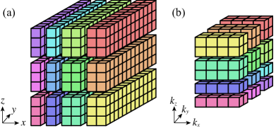
Figure 1: Schematic of pencil decomposition in Calliope. (a) and (b) correspond to the physical and Fourier space grids, respectively.

We now describe the array layout of the field variables. Calliope solves the time evolution of the fields in the Fourier space while the physical space is used only to evaluate the nonlinear terms. In pencil decomposition, one dimension of the three-dimensional array is not distributed between MPI processes, i.e., the array is localized in that direction. As shown in Fig. 1, the $y$-direction in physical space and the $k_{x}$-direction in Fourier space are localized. This choice is to avoid unnecessary transposition or inter-process communication during the remapping process, as described below. Since Calliope uses the stride-1 data structure of P3DFFT, the array layout in each process is:

$$\begin{array}[]{c}\text{Physical space}\\ \left(N^{(l)}_{y},\,N^{(l)}_{z}/M_{1},\,N^{(l)}_{x}/M_{2}\right)\end{array}\;\;\Longleftrightarrow\;\ \begin{array}[]{c}\text{Fourier space}\\ \left(N^{(k)}_{x},\,N^{(k)}_{z}/M_{2},\,N^{(k)}_{y}/M_{1}\right)\end{array}$$

where $N^{(l)}_{x},N^{(l)}_{y}$, and $N^{(l)}_{z}$ are the numbers of grids in physical space, and $N^{(k)}_{x}=2N^{(l)}_{x}/3,N^{(k)}_{y}=N^{(l)}_{y}/3+1$, and $N^{(k)}_{z}=2N^{(l)}_{z}/3$ are the numbers of grids in Fourier space. In addition, $M_{1}M_{2}$ represents the total number of processes.

Next, the remapping method is described. In Calliope, the periodic remapping method (Rogallo, 1981; Umurhan & Regev, 2004) is used for isothermal compressible MHD and incompressible MHD. This method is also used in the SNOOPY code. In shearing coordinates, the wavenumber in the $x$-direction evolves in time according to $k_{x}(t)=k_{x}+q\Omega tk_{y}$. To prevent $k_{x}(t)$ from growing limitlessly, remapping is performed every $T=L_{y}/q\Omega L_{x}$. The fields that are periodic in the $x$-direction in the non-shearing coordinate system at $t=0$ become periodic again in the $x$-direction in the non-shearing coordinate system at $t=T$. Thus, we can rearrange the field such that:

$$f(k_{x},\,k_{y},\,k_{z})\mapsto f(k_{x}+k_{y}L_{x}/L_{y},\,k_{y},\,k_{z}).$$ (6)

Simultaneously, we reset $k_{x}(T)$ to $k_{x}(0)$. With this rearrangement, the data outside the computational domain are discarded, and the portion newly allocated to the computational domain is initialized to zero. Thus, the time evolution of the model becomes somewhat choppy before and after remapping. Since the array is rearranged in the $k_{x}$ direction upon remapping, and Calliope localizes the array in the $k_{x}$ direction, data does not need to be transferred between processors when remapping.

Note, finally, that Calliope is currently limited to periodic boundary conditions in all three directions. P3DFFT can support a Chebyshev transform in one direction allowing non-periodic boundaries while the other two directions are Fourier transformed. This set of transforms is useful to solve systems in a spherical shell. Implementation of a Chebyshev transform in Calliope should be conducted in the future.

4 Tests

In this section, we show the results of linear and nonlinear tests and demonstrate the parallel performance of Calliope.

4.1 Linear wave propagation in isothermal MHD

As a first relatively simple test, we calculate linear wave propagation in isothermal compressible MHD. We set the uniform background magnetic field $(0,0,B_{0})$, the uniform background density $\rho_{0}$, and the wavenumber vector $(k_{x},0,k_{z})$. The initial perturbations of the fields are set to the eigenfunctions of the Alfvén, slow, and fast modes, as shown below (Goedbloed & Poedts, 2004)

• Alfvén mode

  $$\frac{B_{y}}{B_{0}}=-\frac{u_{y}}{v_{\mathrm{A}}},\;\;u_{x}=u_{z}=B_{x}=B_{z}=\rho=0$$

• Slow and fast modes

  $$\frac{\rho}{\rho_{0}}=\left(\frac{\alpha_{\mathrm{s},\mathrm{f}}\omega_{\mathrm{s},\mathrm{f}}}{k_{x}v_{\mathrm{A}}}\right)\left(\frac{v_{\mathrm{A}}}{c_{\mathrm{S}}}\right)^{2}\frac{u_{x}}{v_{\mathrm{A}}},\;\;\frac{B_{z}}{B_{0}}=\frac{k_{x}u_{x}}{\omega_{\mathrm{s},\mathrm{f}}},\;\;$$

  $$u_{z}=\frac{\alpha_{\mathrm{s},\mathrm{f}}k_{\|}}{k_{x}}u_{x},\;\;u_{y}=B_{y}=0,$$

where $\omega_{\mathrm{s},\mathrm{f}}$ is the frequency of the slow and fast modes:

$$\omega_{\mathrm{s},\mathrm{f}}=k\sqrt{\frac{1}{2}\left[v_{\mathrm{A}}^{2}+c_{\mathrm{S}}^{2}\pm\sqrt{\left(v_{\mathrm{A}}^{2}+c_{\mathrm{S}}^{2}\right)^{2}-4\left(k_{z}^{2}/k^{2}\right)v_{\mathrm{A}}^{2}c_{\mathrm{S}}^{2}}\right]}$$

and $\alpha_{\mathrm{s},\mathrm{f}}=1-k^{2}v_{\mathrm{A}}^{2}/\omega_{\mathrm{s},\mathrm{f}}^{2}$. The subscripts s and f denote the slow and fast modes, corresponding to the minus and plus signs in the above equation, respectively. We initialize a mode with one of these eigenfunctions and compute the time evolution to obtain the frequency. We test cases where the value of $\beta\equiv 8\pi\rho_{0}c_{\mathrm{S}}^{2}/B_{0}^{2}$ is 0.1, 1, and 10 by fixing $k_{x}L=1$ and varying $k_{z}$, and by fixing $k_{z}L=1$ and varying $k_{x}$. Figure 2 shows the results of these tests. In all cases, the numerically obtained frequencies accurately reproduce the theoretical values.

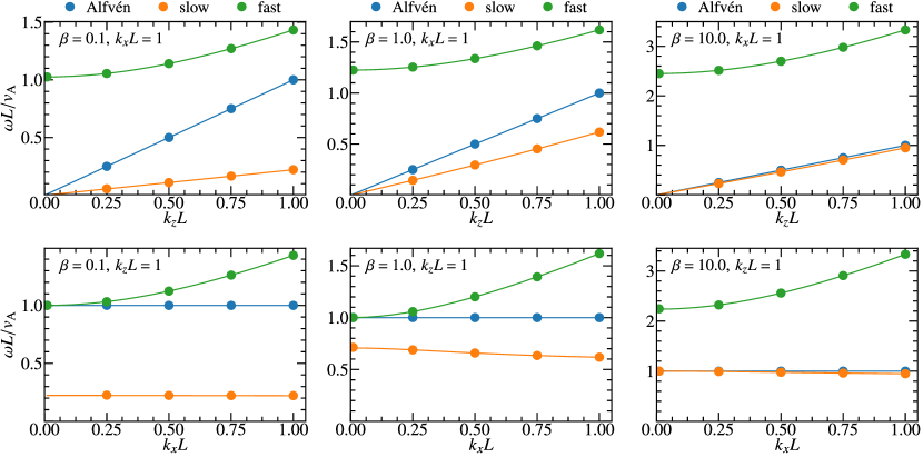
Figure 2: Linear wave propagation test of isothermal compressible MHD. Markers are numerically obtained frequencies, and solid lines are theoretical values.

4.2 Axisymmetric linear MRI in incompressible MHD

Next, we present a test of an axisymmetric ($k_{y}=0$) linear MRI in incompressible MHD. The initial magnetic field is set to $(0,0,B_{0})$. The wavenumber is considered only in the $z$-direction. In this case, the eigenfunctions of the MRI are given by:

$$B_{y}=\left[\frac{\omega^{2}-(k_{z}v_{\mathrm{A}})^{2}+2q\Omega^{2}}{2\mathrm{i}\Omega\omega}\right]B_{x},\;\;B_{z}=0,$$

$$u_{x}=-\frac{\omega}{k_{z}}\frac{B_{x}}{B_{0}},\;\;u_{y}=-\frac{1}{k_{z}}\left(\omega\frac{B_{y}}{B_{0}}+\mathrm{i}q\Omega\frac{B_{x}}{B_{0}}\right),\;\;u_{z}=0,$$

where

$$\omega=\mathrm{i}\gamma=\mathrm{i}\sqrt{\sqrt{4\left(k_{z}v_{\mathrm{A}}\right)^{2}\Omega^{2}+(2-q)\Omega^{4}}-\left(k_{z}v_{\mathrm{A}}\right)^{2}-(2-q)\Omega^{2}},$$ (7)

and $\gamma$ is the growth rate of the MRI. One mode is initialized with this eigenfunction, and the time evolution is calculated to obtain the growth rate. As shown in Fig. 3, the numerically computed growth rates accurately reproduce the theoretical values.

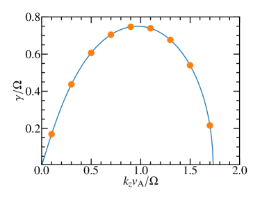
Figure 3: Axisymmetric linear MRI test of incompressible MHD. Markers indicate the numerically obtained growth rates, and the solid line represents the theoretical values.

4.3 Two-dimensional Orszag–Tang vortex problem of RMHD

In the following section, we present the tests of nonlinear simulations. First, we compute the two-dimensional Orszag-–Tang problem using the RMHD model (Orszag & Tang, 1979). We initialize $\Phi$ and $\Psi$ as follows:

$$\Phi = -u_{0}\left(\frac{L_{\perp}}{2\pi}\right)\left[\cos\left(\frac{2\pi x}{L_{\perp}}\right)+\cos\left(\frac{2\pi y}{L_{\perp}}\right)\right],$$

$$\Psi = -u_{0}\left(\frac{L_{\perp}}{2\pi}\right)\left[\frac{1}{2}\cos\left(\frac{4\pi x}{L_{\perp}}\right)+\cos\left(\frac{2\pi y}{L_{\perp}}\right)\right],$$ (8)

where $u_{0}$ is the initial speed, and $L_{\perp}$ is the size of $x$ and $y$ directions. Hyperdissipation proportional to $\nabla_{\perp}^{8}$ is used to terminate the turbulent cascade. Figure 4 shows the results of the test with $(n^{(l)}_{x},\,n^{(l)}_{y})=(2048,\,2048)$. In Fig. 4-(a), we plot each term of the time evolution of free energy:

$$W_{\mathrm{tot}}=W_{u_{\perp}}+W_{\delta B_{\perp}}=\frac{1}{2}\int\mathrm{d}^{3}{\mathbf{r}}\,\left(|\nabla_{\perp}\Phi|^{2}+|\nabla_{\perp}\Psi|^{2}\right),$$ (9)

and power balance:

$$\frac{\mathrm{d}W_{\mathrm{tot}}}{\mathrm{d}t}=-D_{\mathrm{tot}},$$ (10)

where $-D_{\mathrm{tot}}$ is the sum of the dissipation due to the hyper-viscosity and hyper-resistivity terms. At early times, the magnetic field energy increases and the kinetic energy decreases, with the magnetic field energy reaching a peak at $t\simeq 2\tau_{0}$ where $\tau_{0}=L_{\perp}/u_{0}$. This behavior is consistent with the results of a simulation by Parashar et al. (2009). When $t\lesssim 2\tau_{0}$, only energy exchange occurs between the magnetic field and flow, with no energy dissipation [lower panel in Fig. 4-(a)]. The cascade then reaches the grid scale at $t\simeq 2\tau_{0}$, and the energy dissipation starts to increase. The magnetic field profile at $t\simeq 6\tau_{0}$ is shown in Fig. 4-(b), where vortices of various sizes ranging from box scale to grid scale are present, indicating that the flow is turbulent. Fig. 4-(c) shows the kinetic and magnetic spectra at $t\simeq 6\tau_{0}$. Both spectra follow $k_{\perp}^{-3/2}$ power law, which is consistent with observations from other studies of two-dimensional freely decaying MHD turbulence (e.g., Biskamp & Schwarz, 2001). The spectra also show that the dissipation is suppressed until the cascade approaches the grid scale, resulting in a wide inertial range.

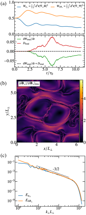
Figure 4: Results of the two-dimensional Orszag–Tang vortex problem using RMHD. (a) Time evolution of magnetic and kinetic energy, and power balance (upper and lower panel, respectively), (b) spatial profile of the magnetic field strength at $t\simeq 6\tau_{0}$, and (c) energy spectra of velocity and magnetic fields. The dashed line shows the $k_{\perp}^{-3/2}$ power law.

4.4 Three-dimensional nonlinear MRI turbulence in isothermal MHD

In this section, we present a test of three-dimensional MRI-driven turbulence in isothermal compressible MHD. This is the first study where compressible MRI turbulence has been simulated using the pseudospectral method, to the best of our knowledge. The sound speed $c_{\mathrm{S}}$, the angular velocity $\Omega$, initial density $\rho_{0}$, and uniform initial magnetic field $(0,0,B_{0})$ are set such that the condition $\lambda_{\mathrm{MRI}}=0.1H$ is satisfied, where $H=c_{\mathrm{S}}/\Omega$ is the scale height of the accretion disk and $\lambda_{\mathrm{MRI}}=2\pi v_{\mathrm{A}}/\Omega$ is approximately equal to the wavelength of the fastest-growing MRI mode (Balbus & Hawley, 1998). The box size is set to $(2H,4H,H)$. The corresponding $\beta$ for this setting is $7.8\times 10^{3}$. The turbulent cascade is terminated with hyper-dissipation proportional to $\nabla^{8}$.

Figure 5 shows the results of a test with $(n^{(l)}_{x},\,n^{(l)}_{y},\,n^{(l)}_{z})=(1024,\,2048,\,512)$. Even though it is a test, the resolution of this simulation is higher than any other previously reported shearing box simulation. In Figure 5-(a), we plot each term of the time evolution of the free energy:

$$W_{\mathrm{tot}}=W_{\mathrm{kin}}+W_{\mathrm{mag}}+W_{\rho}=\int\mathrm{d}^{3}{\mathbf{r}}\left(\frac{\rho u^{2}}{2}+\frac{B^{2}}{8\pi}+c_{\mathrm{S}}^{2}\,\rho\ln\rho\right),$$ (11)

and power balance:

$$\frac{\mathrm{d}W_{\mathrm{tot}}}{\mathrm{d}t}=P_{\mathrm{MRI}}-D_{\mathrm{total}},$$ (12)

where

$$P_{\mathrm{MRI}}=q\Omega\int\mathrm{d}^{3}{\mathbf{r}}\left(\rho u_{x}u_{y}-\frac{B_{x}B_{y}}{4\pi}\right)$$ (13)

is the MRI energy injection rate and $D_{\mathrm{total}}$ is the sum of the hyper-dissipation for ${\mathbf{M}}$, ${\mathbf{B}}$, and $\rho$. As shown in Figure 5-(a), when $t\Omega\lesssim 10$, the MRI grows linearly and then transitions to a nonlinearly saturated state. This figure also illustrates that the power balance is precisely maintained at any given time in the simulation.

Figure 5-(b) shows the spatial profile of magnetic field strength on the $x=0$, $y=0$, and $z=0$ planes. The structure shows clear elongation in the $y$-direction, due to the stretching caused by shear flow in the $y$ direction, being consistent with other shearing box simulations.

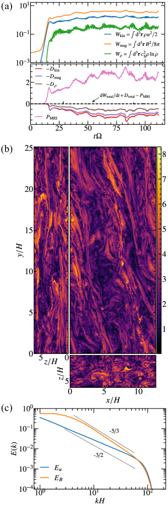
Figure 5: Results of the three-dimensional MRI-driven turbulence in isothermal compressible MHD. (a) Time evolution of the energy and power balance (upper and lower panels, respectively), (b) spatial profile of the magnetic field strength, and (c) energy spectra of the velocity and magnetic fields. The dashed lines show the $k^{-3/2}$ and $k^{-5/3}$ power laws.

Finally, Fig. 5-(c) shows the omni-directional energy spectra of the velocity and the magnetic field. The velocity field is shallower than $k^{-3/2}$ and the magnetic field is slightly steeper than $k^{-5/3}$. These are consistent with the spectra found in previous shearing box simulations (e.g., Sun & Bai, 2021). In addition, since the cascade is terminated with hyper-dissipation proportional to $\nabla^{8}$, the dissipation is suppressed until the cascade approaches the grid scale.

4.5 Parallel Performance

Finally, we describe the parallel performance of Calliope. In the pseudospectral method, most of the computation time is consumed evaluating the nonlinear terms using the FFTs and inverse FFTs. Therefore, the parallel performance of Calliope is mostly determined by that of P3DFFT . Here, the parallel performance was measured for nonlinear incompressible MHD simulations with $(n^{(l)}_{x},\,n^{(l)}_{y},\,n^{(l)}_{z})=(2048,\,2048,\,2048)$. Note that in the case of isothermal compressible MHD, only one forward FFT is added for $\rho$ while the number of inverse FFT remains unchanged, so the scaling is presumably almost the same as that for incompressible MHD. The measurements were carried out on Oakforest-PACS at the University of Tokyo and Fugaku (the Japanese flagship supercomputer as of 2021) at RIKEN. The highest performance was obtained when the number of threads was $N_{\mathrm{thread}}=4$ on Oakforest-PACS and $N_{\mathrm{thread}}=8$ on Fugaku. We fixed the number of threads at these values and measured the execution time upon changing the number of MPI processes, $N_{\mathrm{proc}}$. Figure 6 shows strong scaling, demonstrating the excellent parallel performance of Calliope. As shown, almost ideal scaling is maintained up to $2\times 10^{5}$ cores at Fugaku.

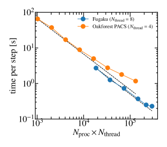
Figure 6: Strong scaling on Oakforest-PACS and Fugaku for incompressible MHD with $(n^{(l)}_{x},\,n^{(l)}_{y},\,n^{(l)}_{z})=(2048,\,2048,\,2048)$. The number of threads is fixed at $N_{\mathrm{thread}}=4$ for Oakforest-PACS and $N_{\mathrm{thread}}=8$ for Fugaku. Dashed lines show the ideal scaling.

In Fig. 6, we chose the aspect ratio of the MPI process grid so that $M_{1}$ and $M_{2}$ become as nearly equal as possible. However, this choice is not always optimal [for example, Pekurovsky (2012, Fig. 3) showed up to 1.44 times performance difference depending on the aspect ratio]. Thus, we measured the performance of Calliope at Oakforest-PACS changing the aspect ratio. The setting was the same as in Fig. 6 (i.e., grid number is fixed to $2048^{3}$, and the thread number is fixed to $N_{\mathrm{thread}}=4$). As shown in Fig. 7, we can barely find the performance difference between the choices of the aspect ratio. Note, however, that the effect of the aspect ratio is supposed to depend on the platform.

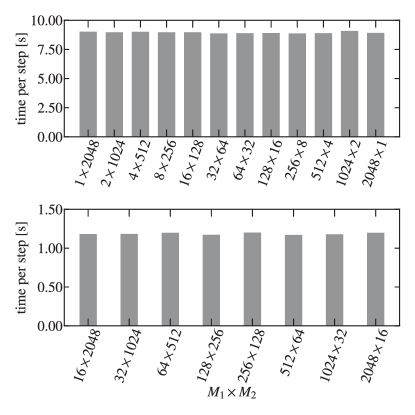
Figure 7: Performance dependence on the aspect ratio of the MPI process grid at Oakforest-PACS. The setting is the same as in Fig. 6. The total number of MPI processes is fixed to (top) $N_{\mathrm{proc}}=2048$ and (bottom) $N_{\mathrm{proc}}=32768$.

5 Summary

This paper has introduced a newly developed open-source code, Calliope, which simulates MHD turbulence with high-order accuracy using the pseudospectral method. Calliope adopts the P3DFFT library to improve the parallel performance of the three-dimensional FFT computation. Due to the pencil decomposition of P3DFFT, almost ideal parallel performance was demonstrated up to $2\times 10^{5}$ processes on the Fugaku supercomputer for $2048^{3}$ grids. We also presented various linear and nonlinear tests to validate the code. In particular, Calliope demonstrated a very narrow dissipation range in nonlinear tests, which is the principal merit of the pseudospectral method. We highlight that this paper has presented the first simulation of MRI-driven turbulence in isothermal compressible MHD using the pseudospectral method. It is anticipated that further interesting properties of MRI-driven turbulence can be identified by analyzing the data obtained in this test.

Moreover, the inertial range in MRI-driven turbulence may be reached using Calliope with increased computational resources. Revealing the nature of the inertial range is crucial for understanding hot accretion disks. For example, it is vital in understanding energy partitioning between ions and electrons (Kawazura et al., 2019, 2020) and the acceleration of non-thermal particles (Kimura et al., 2016; Sun & Bai, 2021). Finally, although this code was developed to simulate MRI-driven turbulence in shearing coordinates, we anticipate that Calliope will be a useful tool for studying other turbulence problems. For example, one can easily modify the RRMHD modules of Calliope to solve Hall RMHD (eqs. (5.14)-(5.17) in Schekochihin et al., 2019), which is a useful model to study turbulence in a regime of electron beta $\sim$ 1 and ion beta $\ll 1$. We hope that this code will be widely used in the future.

References

- Balbus & Hawley (1991) Balbus, S. A., & Hawley, J. F. 1991, ApJ, 376, 214
- Balbus & Hawley (1998) —. 1998, Rev. Mod. Phys., 70, 1
- Biskamp & Schwarz (2001) Biskamp, D., & Schwarz, E. 2001, Physics of Plasmas, 8, 3282
- Bodo et al. (2008) Bodo, G., Mignone, A., Cattaneo, F., Rossi, P., & Ferrari, A. 2008, A&A, 487, 1
- Boldyrev (2006) Boldyrev, S. 2006, Phys. Rev. Lett., 96, 115002
- Brucker et al. (2007) Brucker, K. A., Isaza, J. C., Vaithianathan, T., & Collins, L. R. 2007, Journal of Computational Physics, 225, 20
- Chael et al. (2018) Chael, A., Rowan, M., Narayan, R., Johnson, M., & Sironi, L. 2018, MNRAS, 478, 5209
- Chen et al. (2011) Chen, C. H. K., Mallet, A., Yousef, T. A., Schekochihin, A. A., & Horbury, T. S. 2011, MNRAS, 415, 3219
- Czechowski et al. (2012) Czechowski, K., Battaglino, C., McClanahan, C., et al. 2012, in Proceedings of the 26th ACM international conference on Supercomputing, 205
- Goedbloed & Poedts (2004) Goedbloed, J. P. H., & Poedts, S. 2004, Principles of Magnetohydrodynamics
- Goldreich & Sridhar (1995) Goldreich, P., & Sridhar, S. 1995, ApJ, 438, 763
- Hawley (2000) Hawley, J. F. 2000, ApJ, 528, 462
- Hawley et al. (1995) Hawley, J. F., Gammie, C. F., & Balbus, S. A. 1995, ApJ, 440, 742
- Heinemann & Papaloizou (2009) Heinemann, T., & Papaloizou, J. C. B. 2009, MNRAS, 397, 64
- Hirai et al. (2018) Hirai, K., Katoh, Y., Terada, N., & Kawai, S. 2018, ApJ, 853, 174
- Hoshino (2015) Hoshino, M. 2015, Phys. Rev. Lett., 114, 061101
- Hosking & Schekochihin (2020) Hosking, D. N., & Schekochihin, A. A. 2020, arXiv e-prints, arXiv:2012.01393
- Hussaini & Zang (1987) Hussaini, M. Y., & Zang, T. A. 1987, Annual Review of Fluid Mechanics, 19, 339
- Iroshnikov (1963) Iroshnikov, P. S. 1963, Astron. Zh., 40, 742
- Karniadakis et al. (1991) Karniadakis, G. E., Orszag, S. A., & Israeli, M. 1991, J. Comp. Phys., 97, 414
- Kawazura & Barnes (2018) Kawazura, Y., & Barnes, M. 2018, Journal of Computational Physics, 360, 57
- Kawazura et al. (2019) Kawazura, Y., Barnes, M., & Schekochihin, A. A. 2019, Proc. Nat. Acad. Sci., 116, 771
- Kawazura et al. (2021) Kawazura, Y., Schekochihin, A. A., Barnes, M., Dorland, W., & Balbus, S. A. 2021, arXiv:2110.12434 [astro-ph.HE]
- Kawazura et al. (2020) Kawazura, Y., Schekochihin, A. A., Barnes, M., et al. 2020, Phys. Rev. X, 10, 041050
- Kempski et al. (2019) Kempski, P., Quataert, E., Squire, J., & Kunz, M. W. 2019, MNRAS, 486, 4013
- Kimura et al. (2016) Kimura, S. S., Toma, K., Suzuki, T. K., & Inutsuka, S.-i. 2016, ApJ, 822, 88
- Kraichnan (1965) Kraichnan, R. H. 1965, Phys. Fluids, 8, 1385
- Kunz & Lesur (2013) Kunz, M. W., & Lesur, G. 2013, MNRAS, 434, 2295
- Kunz et al. (2016) Kunz, M. W., Stone, J. M., & Quataert, E. 2016, Phys. Rev. Lett., 117, 235101
- Lesur & Longaretti (2007) Lesur, G., & Longaretti, P. Y. 2007, MNRAS, 378, 1471
- Lesur & Longaretti (2011) —. 2011, A&A, 528, A17
- Lithwick (2007) Lithwick, Y. 2007, ApJ, 670, 789
- Loureiro & Boldyrev (2017) Loureiro, N. F., & Boldyrev, S. 2017, Phys. Rev. Lett., 118, 245101
- Loureiro et al. (2016) Loureiro, N. F., Dorland, W., Fazendeiro, L., et al. 2016, Computer Physics Communications, 206, 45
- Machida et al. (2000) Machida, M., Hayashi, M. R., & Matsumoto, R. 2000, ApJ, 532, L67
- Mallet et al. (2017) Mallet, A., Schekochihin, A. A., & Chandran, B. D. G. 2017, MNRAS, 468, 4862
- Mininni et al. (2011) Mininni, P. D., Rosenberg, D., Reddy, R., & Pouquet, A. 2011, Parallel Computing, 37, 316
- Numata et al. (2010) Numata, R., Howes, G. G., Tatsuno, T., Barnes, M., & Dorland, W. 2010, Journal of Computational Physics, 229, 9347
- Orszag (1969) Orszag, S. A. 1969, Physics of Fluids, 12, II
- Orszag & Tang (1979) Orszag, S. A., & Tang, C. M. 1979, Journal of Fluid Mechanics, 90, 129
- Parashar et al. (2009) Parashar, T. N., Shay, M. A., Cassak, P. A., & Matthaeus, W. H. 2009, Physics of Plasmas, 16, 032310
- Pekurovsky (2012) Pekurovsky, D. 2012, SIAM Journal on Scientific Computing, 34, C192
- Perrone & Latter (2021a) Perrone, L. M., & Latter, H. 2021a, arXiv:2110.13918 [astro-ph.CO]
- Perrone & Latter (2021b) —. 2021b, arXiv:2110.14696 [astro-ph.CO]
- Ressler et al. (2015) Ressler, S. M., Tchekhovskoy, A., Quataert, E., Chandra, M., & Gammie, C. F. 2015, MNRAS, 454, 1848
- Rogallo (1981) Rogallo, R. S. 1981, Numerical experiments in homogeneous turbulence, NASA STI/Recon Technical Report N
- Sano et al. (2004) Sano, T., Inutsuka, S.-i., Turner, N. J., & Stone, J. M. 2004, ApJ, 605, 321
- Schekochihin (2020) Schekochihin, A. A. 2020, arXiv:2010.00699, arXiv:2010.00699 [physics.plasm-ph]
- Schekochihin et al. (2009) Schekochihin, A. A., Cowley, S. C., Dorland, W., et al. 2009, ApJS, 182, 310
- Schekochihin et al. (2019) Schekochihin, A. A., Kawazura, Y., & Barnes, M. A. 2019, J. Plasma Phys., 85, 905850303
- Sharma et al. (2006) Sharma, P., Hammett, G. W., Quataert, E., & Stone, J. M. 2006, ApJ, 637, 952
- Sądowski et al. (2017) Sądowski, A., Wielgus, M., Narayan, R., et al. 2017, MNRAS, 466, 705
- Squire & Bhattacharjee (2015) Squire, J., & Bhattacharjee, A. 2015, Phys. Rev. Lett., 115, 175003
- Squire et al. (2020) Squire, J., Chandran, B. D. G., & Meyrand, R. 2020, ApJ, 891, L2
- St-Onge et al. (2020) St-Onge, D. A., Kunz, M. W., Squire, J., & Schekochihin, A. A. 2020, J. Plasma Phys., 86, 905860503
- Sun & Bai (2021) Sun, X., & Bai, X.-N. 2021, MNRAS, 506, 1128
- Suzuki & Inutsuka (2014) Suzuki, T. K., & Inutsuka, S.-i. 2014, ApJ, 784, 121
- Tchekhovskoy et al. (2011) Tchekhovskoy, A., Narayan, R., & McKinney, J. C. 2011, MNRAS, 418, L79
- Umurhan & Regev (2004) Umurhan, O. M., & Regev, O. 2004, A&A, 427, 855
- Walker & Boldyrev (2017) Walker, J., & Boldyrev, S. 2017, MNRAS, 470, 2653
- Walker et al. (2016) Walker, J., Lesur, G., & Boldyrev, S. 2016, MNRAS, 457, L39
- Zhdankin et al. (2017) Zhdankin, V., Walker, J., Boldyrev, S., & Lesur, G. 2017, MNRAS, 467, 3620