The Inverse Problem for Controlled Differential Equations

Abstract.

We study the problem of constructing the control driving a controlled differential equation from discrete observations of the response. By restricting the control to the space of piecewise linear paths, we identify the assumptions that ensure uniqueness. The main contribution of this paper is the introduction of a novel numerical algorithm for the construction of the piecewise linear control, that converges uniformly in time. Uniform convergence is needed for many applications and it is achieved by approaching the problem through the signature representation of the paths, which allows us to work with the whole path simultaneously.

Keywords : Controlled Differential Equations, Inverse Problems, Rough Path Signature.

1. Introduction

Consider the controlled differential equation (CDE)

(1) $$dY_{t}=f(Y_{t})\cdot dX_{t},\ \ Y_{0}=y_{0},\ 0\leq t\leq T.$$

where the control $X\in\Omega_{p}({}^{m})$ is a $p$-rough path and the vector field $f:{}^{d}\to L\left({}^{m},{}^{d}\right)$ is ${\rm Lip}(\gamma)$, for $\gamma>p\geq 1$. Then, the solution $Y$ exists and it is also a rough path in $\Omega_{p}({}^{d})$ [11, 4]. The CDE (1) defines an Itô map $I:\Omega_{p}({}^{m})\to\Omega_{p}({}^{d})$, mapping a rough path $X$ to a rough path $Y$, which is continuous in $p$-variation topology [11, 4].

The motivating question for this paper is how to extract information about either the control $X$ or the vector field $f$, from discrete observations of the solution (response) $Y$. This question comes up in numerous applications and takes many different forms, depending on the assumptions. One common assumption is that $X$ is a realisation of a Brownian path (and possibly, time) and $f$ belongs to a parametric family, which corresponds to the well-studied problem of statistical inference for discretely observed diffusions [10]. More generally, we are often asked to make inference about the vector field, when $X$ is a realisation of a random rough path with known distribution [6, 14]. Recently, CDEs were used to model recurrent neural networks, where the aim is to learn the vector field when observing both $X$ and $Y$ [8].

The dual problem to making inference about the vector field $f$ is reconstructing the control $X$, assuming that the vector field is known. This can be of independent interest, allowing, for example, one to make inference about the distribution of the random control $X$ driving the system [9]. It also provides an indirect way of learning the vector field: in the case where the control is a realisation of a random path with known distribution, reconstructing the path $X$ conditioned on the vector field $f$ can lead to the construction of an approximate likelihood [12]. In the context of neural CDEs where the input $X$ is unobserved, there are situations where the same unobserved control $X$ could be applied to a known system, thus making it possible to first infer $X$ and then use existing methods for learning the vector field [8]. Thus, we focus on the following problem: how can we construct a path $\hat{X}$ whose response, when driving (1), is consistent with discrete observations $\bar{Y}_{\mathcal{D}}=\{Y_{0},Y_{t_{1}},\dots,Y_{t_{N}}=Y_{T}\}$ of the solution $Y$ of (1) on a partition ${\mathcal{D}}=\{t_{0}=0,t_{1},\dots,t_{N}=T\}$ of $[0,T]$? In other words, how do we solve the inverse problem for CDEs? This has also been studied in [1], but in a different context: the authors reconstruct the truncated signature of the control $X$ on a fixed window from observations of the increments of the solution to the CDE on that window for a number of different initial conditions.

Clearly, as posed, the solution $\hat{X}$ to the inverse problem is not unique. As a first step towards providing a general methodology for addressing the question above, we will restrict the search for the path $\hat{X}$ to the family of piecewise linear paths on ${\mathcal{D}}$. The formulation of the problem at the level of paths leads to a localised approach, expressing each linear segment of the piecewise linear path $\hat{X}$ as a solution to a system of equations involving the solution to a Partial Differential Equation (PDE). In section 2, we study uniqueness of the path $\hat{X}$ by studying uniqueness of the corresponding system of equations.

In section 3, we present a numerical algorithm for the construction of the solution to the inverse problem, assuming uniqueness and existence. Our goal is to construct an algorithm that convergences uniformly with respect to the number of observations $N$, which will depend on time horizon $T$ or observation frequency $\delta$. Uniform convergence is necessary, in order to construct an approximate solution of the general inverse problem, when $X$ is a $p$-rough path. In subsection 3.1, we argue that any numerical algorithm that solves the problem locally does not guarantee uniform convergence, as the $L_{\infty}$ error of the approximate path constructed by joining all the constructed linear segments grows with $N$. To achieve uniform convergence, we need a different formulation of the problem, in terms of the whole path, which is provided by its signature representation (in a rough path sense [11]). In subsection 3.2, we present a novel and powerful algorithm based on signatures, whose error can be controlled pathwise. The main idea is to iterate between the driving path $X$ and the solution $Y$ by applying the corresponding Itô and inverse Itô map, each time correcting the resulting paths $X$ and $Y$ so that they satisfies requirements, in a way that changes their signature as little as possible. We reformulate the algorithm in terms of paths, making it easier to study and implement, while retaining all the advantages. Finally, in section 4, we present numerical experiments, where the performance of the signature-based algorithm is compared to classical algorithms.

2. Set-up and Uniqueness

Let $Y\in\Omega_{p}({}^{d})$ be the solution (response) of (1) driven by a $p$-rough path $X\in\Omega_{p}({}^{m})$, with $f\in{\rm Lip}(\gamma)$, for $\gamma>p$. We denote by $\bar{Y}_{\mathcal{D}}=\{Y_{t_{i}},t_{i}\in{\mathcal{D}}\}$ the values of $Y$ on ${\mathcal{D}}$. Partition ${\mathcal{D}}$ can be arbitrary but, for ease of notation, we will assume that it is homogeneous, so ${\mathcal{D}}=\{0,\delta,2\delta,\dots,N\delta=T\}$ for some $\delta>0$. We define the inverse problem as follows:

Definition 2.1 (Inverse Problem).

Given a vector $\bar{Y}_{\mathcal{D}}=\{Y_{t_{i}},t_{i}\in{\mathcal{D}}\}\in\left({}^{d}\right)^{\otimes|{\mathcal{D}}|}$ and a vector field $f$ as above, find a path $\hat{X}$ such that

• $\hat{X}$ is a piecewise linear path on ${\mathcal{D}}$ starting at $\hat{X}_{0}=0$.

• $\hat{Y}=I(\hat{X})$, where $I$ is the Itô map defined by (1), i.e. $\hat{Y}$ is the solution to

  (2) $$d\hat{Y}_{t}=f(\hat{Y}_{t})\cdot d\hat{X}_{t},\ 0\leq t\leq T,\ \ \hat{Y}_{0}=Y_{0}.$$

• $\hat{Y}_{t_{i}}=Y_{t_{i}},\ \forall t_{i}\in{\mathcal{D}}$.

That is, we are looking for a piecewise linear path $\hat{X}$ whose response through (1) matches the observations. First, we ask the question of existence and uniqueness. Since $\hat{X}$ is piecewise linear on ${\mathcal{D}}$, we can write it as

(3) $$\hat{X}_{t}=\hat{X}_{k\delta}+c_{k+1}(t-k\delta),\ \ {\rm for}\ t\in[k\delta,(k+1)\delta],k=0,1,\dots,N-1.$$

So, (2) can be re-written as a sequence of equations

(4) $$d\hat{Y}_{t}=\left(f(\hat{Y}_{t})\cdot c_{k}\right)dt,t\in[(k-1)\delta,k\delta],$$

with initial condition $\hat{Y}_{0}=Y_{0}$. The solution can be constructed by solving repeatedly equation

(5) $$d\tilde{Y}_{t}=\left(f(\tilde{Y}_{t})\cdot c\right)dt,t\in[0,\delta],$$

for $c=c_{k}$, for each $k=1,\dots,N$ and with initial conditions chosen to match terminal values on the preceding interval. Since $f\in{\rm Lip}(\gamma)$ with $\gamma>1$, the solution to (5) exists and it is unique. We denote it by $F\left(t;y,c\right)$, where $y$ is the initial condition and $c$ the constant now incorporated into the new vector field $f\cdot c$. Then, for $t\in[k\delta,(k+1)\delta]$,

(6) $$\hat{Y}_{t}=F(t-k\delta;\hat{Y}_{k\delta},c_{k+1}).$$

With $\hat{X}$ and $\hat{Y}$ expressed as (3) and (6) respectively, conditions (a) and (b) in the definition 2.1 of the inverse problem are satisfied, while condition (c) gives the initial and terminal values for (6), becoming

(7) $$Y_{(k+1)\delta}=F(\delta;Y_{k\delta},c_{k+1}).$$

As $\hat{X}$ is completely determined by the vector ${\bf c}=\left(c_{k}\right)_{k=1}^{N}$, we can study its existence and uniqueness by studying the existence and uniqueness of solutions to equation (7). To this end, we state

Proposition 2.2.

Let ${\mathcal{D}}=\{0,\delta,2\delta,\dots,N\delta=T\}$ for some $\delta>0$ and let $\bar{Y}_{\mathcal{D}}=(Y_{k\delta})_{k=1}^{N}$ be a sequence of points in ^d. Suppose that $m\geq d$ and that $f\in{\rm Lip}(2)$. Moreover, we assume that ${\rm rank}\left(f(y)\right)=d$ for every $y\in{}^{d}$, and that the solution to (7) exists for all $k=1,\dots,N$. Then, the solution for each $k=1,\dots,N$ will also be unique if $m=d$, and it will have $(m-d)$-degrees of freedom if $m>d$.

Before proving proposition 2.2, we prove the following

Lemma 2.3.

Consider the initial value problem

(8) $$d\tilde{Y}_{t}=\left(f(\tilde{Y}_{t})\cdot c\right)dt,\tilde{Y}_{0}=y,$$

where $f:{}^{d}\to L({}^{m},{}^{d})$ is ${\rm Lip}(2)$, $c\in{}^{m}$ and $y\in{}^{d}$. Let $\tilde{Y}_{t}=F(t;y,c)$ be the solution to (8) and $\tilde{Z}_{t}=G(t;y,c)$ be the derivative of the solution with respect to $c$, i.e.

(9) $$G(t;y,c)=\bigtriangledown_{c}F(t;y,c)\in{}^{d\times m}.$$

Then, if ${\rm rank}\left(f(y)\right)=\min(d,m)$ for all $y$, it follows that for every $t>0$,

$${\rm rank}\left(G(t;y,c)\right)=\min(d,m).$$

Proof.

The vector field $f\cdot c$ of (8) is linear with respect to $c$ and ${\rm Lip}(2)$ with respect to $y$, and thus it is continuously differentiable and the solution to (8) exists. So, the solution $F(t;y,c)$ will also be continuously differentiable with respect to $c$ for every $y$ and $t$ ([3] or [7], Theorem 8.49). Moreover, the process $\tilde{Z}_{t}$ is well-defined and it satisfies

(10) $$\frac{d}{dt}\tilde{Z}_{t}=A(\tilde{Y}_{t};c)\cdot\tilde{Z}_{t}+f(\tilde{Y_{t}}),$$

where

(11) $$A(y;c)=\left(\bigtriangledown_{y}f(y)\right)\cdot c,$$

and $\bigtriangledown_{y}f\in{}^{d\times d\times m}$. Note that (10) is a linear equation of $\tilde{Z}_{t}$ with non-homogeneous coefficients, with initial conditions given by

$$\tilde{Z}_{0}=G(0;y_{0},c)=\bigtriangledown_{c}F(0;y_{0},c)=\bigtriangledown_{c}y_{0}\equiv{\bf 0}_{d\times m},$$

where ${\bf 0}_{d\times m}$ is the $d\times m$-matrix with all entries equal to $0$. Thus, the solution to this equation will be

(12) $$\tilde{Z}_{t}=\int_{0}^{t}\exp\left(\int_{s}^{t}A(\tilde{Y}_{u};c)du\right)f(\tilde{Y}_{s})ds.$$

Using the continuity of the integrated function with respect to $s$, we can write

$$\tilde{Z}_{t}=\exp\left(\int_{\xi}^{t}A(\tilde{Y}_{u};c)du\right)f(\tilde{Y}_{\xi})t,$$

for some $\xi\in(0,t)$. As the exponential $d\times d\times m$ matrix is always invertible (for $\xi<t$), the rank of the product of the two matrices will be equal to the rank of $f$, which proves the result. ∎

Now, we can prove proposition 2.2.

Proof.

We have already seen that for every interval $k=1,\dots,N$, $c_{k}$ is the solution to (7). Without loss of generality, it is sufficient that we study the uniqueness of the solution to the first interval corresponding to system

$$y_{1}=F(\delta;y_{0},c).$$

Suppose that both $c_{1}$ and $c_{2}$ solve the system above, i.e.

$$F(\delta;y_{0},c_{1})=y_{1}=F(\delta;y_{0},c_{2}).$$

We can write the difference as

$$F(\delta;y_{0},c_{2})-F(\delta;y_{0},c_{1})=\left(\int_{0}^{1}\bigtriangledown_{c}F(\delta;y_{0},c_{1}+s(c_{2}-c_{1}))ds\right)\cdot(c_{2}-c_{1}).$$

Thus, $F(\delta;y_{0},c_{1})=F(\delta;y_{0},c_{2})$ implies

$$\left(\int_{0}^{1}\bigtriangledown_{c}F(\delta;y_{0},c_{1}+s(c_{2}-c_{1}))ds\right)\cdot(c_{2}-c_{1})=0.$$

So, it is sufficient to show that $\forall\xi\in{}^{m}$, the rank of matrix $\bigtriangledown_{c}F(\delta;y_{0},\xi)$ is $d$, which implies that the solution will have $m-d$ degrees of freedom, i.e. given $m-d$ coordinates of $c$, the other coordinates are uniquely defined. In particular, for $d=m$ we get uniqueness. This follows from lemma 2.3, as $\bigtriangledown_{c}F(\delta;y_{0},\xi)=G(\delta;y_{0},\xi)$.

∎

3. Numerical Algorithms

For the remaining paper, we will assume $m=d$ and existence and uniqueness of the solution to $\eqref{eq:c}$ for every $k=1,\dots,N$, which is equivalent to the existence and uniqueness of the solution to the inverse problem stated in definition 2.1. When the solution $c$ to (7) has an exact closed-form expression, then this will correspond to a piecewise linear path that solves the inverse problem. However, in most cases, an analytic solution doesn’t exist and we need to resort to numerical approximations. Note that, while connected, our goal is not to solve (7) but to construct the piecewise linear path $\hat{X}$. So, if $\hat{X}(n)$ is an approximation of $\hat{X}$ corresponding to constants ${\bf c}(n)=\left(c(n)_{k}\right)_{k=1}^{N}$, we define the total error of the approximation as the $L_{\infty}$-distance between $\hat{X}$ and $\hat{X}(n)$, i.e.

(13) $$e(n;T)=\sup_{{t\in[0,T]}}|\hat{X}_{t}-\hat{X}(n)_{t}|.$$

It follows from (3) that for $t\in[k\delta,(k+1)\delta]$,

$$\hat{X}_{t}=\left(\sum_{j=1}^{k}c_{j}\right)\delta+c_{k+1}(t-k\delta)$$

and similarly for $\hat{X}(n)$. So,

$$\hat{X}_{t}-\hat{X}(n)_{t}=\left(\sum_{j=1}^{k}(c_{j}-c(n)_{j})\right)\delta+(c_{k+1}-c(n)_{k+1})(t-k\delta).$$

Noting that for piecewise linear paths the $L_{\infty}$-distance over each linear segment will be maximised on one of their endpoints, the error can be expressed in terms of vectors ${\bf c}$ and ${\bf c}(n)$ as

(14) $$\tilde{e}(n;T,\delta)=\sup_{k=1,\dots,N}\left|\sum_{j=1}^{k}(c_{j}-c(n)_{j})\right|\delta.$$

Depending on the context, we will require the error to disappear uniformly, with respect to $N=\frac{T}{\delta}$.

3.1. Classical approach

The first natural idea for constructing a numerical approximation to $\hat{X}$ is to try and approximate the solution to (7) for each $k=1,\dots,N$. This is a standard problem that involves numerically solving a system of equations and an ODE. For example, applying the Newton-Raphson algorithm in the context of (7) gives

(15) $$c(n+1)_{k} = c(n)_{k}+D_{c}F(\delta;Y_{k\delta},c(n)_{k})^{-1}\left(Y_{k\delta}-F(\delta;Y_{k\delta},c(n)_{k})\right)$$

$$= c(n)_{k}+G(\delta;Y_{k\delta},c(n)_{k})^{-1}\left(Y_{k\delta}-F(\delta;Y_{k\delta},c(n)_{k})\right).$$

Both $\tilde{Y}_{\delta}=F(\delta;Y_{k\delta},c(n)_{k}))$ and $\tilde{Z}_{\delta}=G(\delta;Y_{k\delta},c(n)_{k})$ are solutions to the system of ODEs consisting of (8) and (10), which can be solved using standard numerical techniques, such as the Euler method with step $\delta^{\prime}<<\delta$. Whatever numerical method we choose for solving (7), the approximation errors $\eta_{k}(n)=\left(c_{k}-c(n)_{k}\right)$ for $k=1,\dots,N$, do not depend on each other and even when they converge to $0$ individually, the total error (14) will be the cumulative error, given by

$$\tilde{e}(n;T,\delta)=\sup_{k=1,\dots,\frac{T}{\delta}}\left|\sum_{j=1}^{k}\eta_{k}(n)\right|\delta=\sup_{k=1,\dots,N}\left|\sum_{j=1}^{k}\eta_{k}(n)\right|\frac{T}{N},$$

which will not, in general, converge to $0$ uniformly in $N>0,T>0$.

3.2. Signature approach

The classical approach fails to lead to a numerical algorithm that converges uniformly in $T>0$ and $N>0$ because it is based on solving equations (7) independently for each $k=1,\dots,N$, thus failing to make use of the assumption of continuity of the piecewise linear path $\hat{X}$. To avoid this shortcoming, we need to move away from (7), reformulating the problem on the path space. The signature of a path $X:[0,T]\to{}^{m}$ is defined as the collection of iterated integrals

(16) $$S(X)_{0,T}:=\left(1,\int_{0}^{T}dX_{u},\underset{0<u_{1}<u_{2}<T}{\int\int}dX_{u_{1}}\otimes dX_{u_{2}},\dots,\underset{0<u_{1}<\cdots<u_{n}<T}{\int\cdots\int}dX_{u_{1}}\otimes\cdots\otimes dX_{u_{n}},\dots\right)$$

belonging to the tensor algebra on ^m, $T({}^{m})$, with the logarithm of the signature (log-signature), ${\rm log}S(X)$ belonging to the corresponding free Lie algebra. We call

$$S(X)_{0,T}^{n}=\underset{0<u_{1}<\cdots<u_{n}<T}{\int\cdots\int}dX_{u_{1}}\otimes\cdots\otimes dX_{u_{n}}\in({}^{m})^{n}$$

the $n^{\rm th}$ level of the signature and we similarly define the $n^{\rm th}$ level of the log-signature [11]. The signature characterises the path, up to tree-like equivalence [2], thus providing an alternative representation of the path. Similarly, we can define the signature of path $Y:[0,T]\to{}^{d}$ and the Itô map corresponding to (1) can be expressed as a linear map ${\bf I}$, mapping $S(X)$ to $S(Y)$.

We can reformulate definition 2.1 of the inverse problem in terms of signatures of paths, as follows:

Definition 3.1 (Inverse problem on signatures).

Given a vector $\bar{Y}_{\mathcal{D}}=\{Y_{t_{i}},t_{i}\in{\mathcal{D}}\}\in\left({}^{d}\right)^{\otimes|{\mathcal{D}}|}$ and a vector field $f\in{\rm Lip}(\gamma)$, for $\gamma>p$, find a path $\hat{X}$ such that

• All but the first coordinate of the log-signature of the path $\hat{X}$ on $[t_{i},t_{i+1}]$ are $0$, which is equivalent to the path being linear on that segment, i.e.

  $${\rm log}S(\hat{X})_{t_{i},t_{i+1}}^{k}=0,\forall t_{i}\in{\mathcal{D}}\ {\rm and}\ \forall k\geq 2.$$

• If ${\bf I}$ is the Itô map defined on signatures, corresponding to (1), then

  $$S(\hat{Y})_{0,T}={\bf I}\cdot S((\hat{X}))_{0,T}.$$

• The first level of the log-signature of $\hat{Y}$ corresponds to the increments given by the observations, i.e.

  $${\rm log}S(\hat{Y})^{1}_{t_{i},t_{i+1}}=Y_{t_{i+1}}-Y_{t_{i}},\ \forall t_{i}\in{\mathcal{D}}.$$

3.2.1. Description of algorithm

We have assumed existence and uniqueness of the path $\hat{X}$ solving the inverse problem, which implies that the Itô map $I$ corresponding to (1) is invertible. In fact, $\hat{X}$ can be expressed as an integral with respect to the rough path $\hat{Y}$: given the path $\hat{Y}$, $\hat{X}$ will be

(17) $$\hat{X}_{t}=\int_{0}^{t}f(\hat{Y}_{u})^{-1}\cdot d\hat{Y}_{u},t\in[0,T].$$

Note that (17) above requires knowledge of the whole continuous path $\hat{Y}$ on $[0,T]$ and not just its values on the partition ${\mathcal{D}}$. Also, since we assumed uniqueness of the solution of the inverse problem, it follows from proposition 2.2 that the inverse of matrix $f(y)$, $f(y)^{-1}$, is well definted.

The main idea of the algorithm is to construct a sequence of rough paths

$$\cdots\to Y(n)\to X(n)\to\tilde{X}(n)\to\tilde{Y}(n+t)\to Y(n+1)\to\cdots$$

each time trying to correct for conditions (a), (b) and (c) of definition 3.1 by applying the smallest possible change to the signature of the corresponding path (see figure 1). While no pair $(X(n),Y(n))$ is expected to satisfy all three conditions, the goal is to construct a contraction map so that $(X(n),Y(n))$ converges to the solution of the inverse problem $(\hat{X},\hat{Y})$. In particular, convergence of the algorithm implies convergence of $\tilde{X}(n)$ to the solution of the inverse problem $\hat{X}$, thus $\tilde{X}(n)$ provides an alternative approximation of $\hat{X}$.

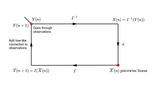
Figure 1. Schematic description of algorithm 1.

More precisely, the algorithm can be described as follows:

Algorithm 1 (on signatures).

Given a vector $\bar{Y}_{\mathcal{D}}=\{Y_{t_{i}},t_{i}\in{\mathcal{D}}\}\in\left({}^{d}\right)^{\otimes|{\mathcal{D}}|}$ and a vector field $f\in{\rm Lip}(\gamma)$, $\gamma>p$, defining the Itô and inverse Itô maps ${I}$ and ${I}^{-1}$ corresponding to (1) and (17) respectively, we construct a sequence of rough paths $(X(n),Y(n))$ as follows:

Step 0 (initialisation):

• Initialise $Y(0)$ as the piecewise linear path going through $\bar{Y}_{\mathcal{D}}$ (see figure 2 (i)). Then, condition (c) of definition 3.1 is satisfied.

Step $n\to n+1$

• Given $Y(n)$ satisfying condition (c) by construction, define $X(n)=I^{-1}((Y(n))$, so that $(X(n),Y(n))$ satisfy conditions (b) and (c) of definition 3.1 (see figure 2 (ii) and (v)), but not condition (a).

• Define $\tilde{X}(n)$ as the projection of $X(n)$ onto the space of piecewise linear paths on ${\mathcal{D}}$ (see figure 2 (ii) and (v)). In terms of signatures, this means that $\forall t_{i}\in{\mathcal{D}}$

  $${\rm log}S(\tilde{X}(n))^{1}_{t_{i},t_{i+1}}={\rm log}S(X(n))^{1}_{t_{i},t_{i+1}}\ \ {\rm and}\ \ {\rm log}S(\tilde{X}(n))^{k}_{[t_{i},t_{i+1}]}=0,\ k\geq 2.$$

  This is the minimum change to the signature on each segment, so that it corresponds to a linear path and $(\tilde{X}(n),Y(n))$ satisfy conditions (a) and (c) but not (b).

• Define $\tilde{Y}(n+1)=I^{-1}(\tilde{X}(n))$, so that $(\tilde{X}(n),\tilde{Y}(n+1))$ satisfies conditions (a) and (b), but it now fails to satisfy (c) (see figure 2 (iii) and (vi)).

• Define $Y(n+1)$ by adding tree-like paths to connect to the observations, i.e. $Y(n+1)$ can be expressed as a concatenation of paths, with each segment corresponding to

  $$Y(n+1)_{t_{i},t_{i+1}}=L(Y_{t_{i}},\tilde{Y}(n+1)_{t_{i}})\otimes\tilde{Y}_{t_{i},t_{i+1}}\otimes L(\tilde{Y}(n+1)_{t_{i+1}},Y_{t_{i+1}}),$$

  where for any two points $y,\tilde{y}\in{}^{d}$, $L(y,\tilde{y})$ is the linear path connecting $y$ to $\tilde{y}$ (see figure 2 (iv)). Then, $(\tilde{X}(n),Y(n+1))$ satisfy (a) and (c), but not (b). Note that by adding a tree-like path connecting to the observations, we are not changing the signature of the path over the whole interval $[0,T]$ [2].

Remark 3.2.

Algorithm 1 assumed that $\hat{X}$ is completely unknown. However, there are many examples where some coordinates of $\hat{X}$ might be known (e.g. when (1) has a drift). In that case, the algorithm remains the same, with the Itô and inverse Itô maps restricted to the unknown coordinates of $\hat{X}$.

While the description above explains the intuition behind the algorithm, it is not very practical to implement. However, it can be simplified by using the piecewise linear assumption on $\tilde{X}(n)$. We can write

(18) $$\tilde{X}(n)_{t}=\tilde{X}_{k\delta}+\tilde{c}(n)_{k}(t-k\delta),\ {\rm for}\ t\in[k\delta,(k+1)\delta],\ k=1,\dots,N-1,$$

The following proposition gives an equivalent way of expressing algorithm 1 as an update on vector ${\bf\tilde{c}}(n)=(\tilde{c}(n)_{k})_{k=1}^{N}$.

Proposition 3.3.

Let ${\bf\tilde{c}}(n)=(\tilde{c}(n)_{k})_{k=1}^{N}$ be defined by the local derivatives of the linear segments of the piecewise linear path $\tilde{X}(n)$ constructed through algorithm 1, so that (18) is satisfied. Then, ${\bf\tilde{c}}(n)=(\tilde{c}(n)_{k})_{k=1}^{N}$ can be constructed directly as follows:

• For each $k=1,\dots,N$,

  (19) $$\tilde{c}(0)_{k}=\int_{(k-1)\delta}^{k\delta}f(Y(0)_{u})^{-1}dY(0)_{u}$$

  where $Y(0)$ is the linear interpolation of the observations, as described in step 0 of algorithm 1.

• Given ${\bf\tilde{c}}(n)$, we define ${\bf\tilde{c}}(n+1)$ by

  (20) $$\tilde{c}(n+1)_{k}=\tilde{c}(n)_{k}+\left(r(n+1)_{k}-r(n+1)_{k-1}\right)$$

  where $\tilde{r}(n+1)_{0}=0$ and for $k=1,\dots,N$,

  (21) $$r(n+1)_{k}=\frac{Y_{k\delta}-\tilde{Y}(n)_{k\delta}}{\delta}\frac{1}{\delta}\int_{0}^{\delta}f\left(L(\tilde{Y}(n)_{k\delta},Y_{k\delta})_{u}\right)^{-1}du.$$

  As in algorithm 1, $L(y,\tilde{y})$ is the linear path connecting $y$ with $\tilde{y}$ and $\tilde{Y}(n)$ is the solution of (1), driven by $\tilde{X}(n)$ corresponding to ${\bf\tilde{c}}(n)$.

Proof.

It follows from a direct computation of the new constants ${\bf\tilde{c}}(n+1)$ following the steps of the algorithm. ∎

Note that algorithm 1 still requires the solution to the ODE (8), which would normally involve using an ODE solver.

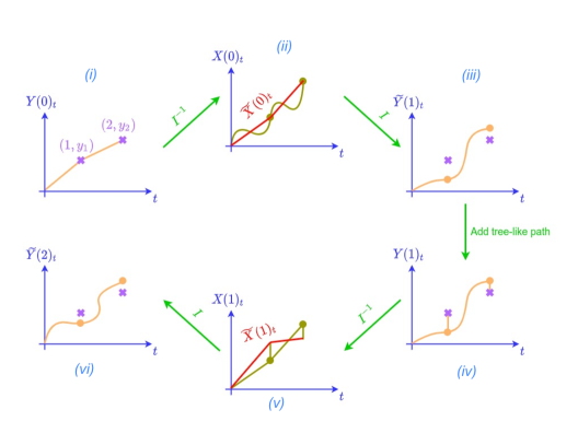
Figure 2. Step-by-step description of algorithm 1.

4. Numerical Examples

We compare the classical approach of subsection 3.1 to the algorithm presented in subsection 3.2. We consider two different models for (1): the Cox-Ingersol-Ross (CIR) model and the Constant Elasticity of Variance (CEV) model, driven by random piecewise linear paths.

4.1. Cox-Ingersoll-Ross model

We consider the system described by

(22) $$d\hat{Y}_{t}=a(b-\hat{Y}_{t})dt+\sigma\sqrt{\hat{Y}_{t}}d\hat{X}_{t},$$

where $\hat{X}_{t}$ is a random piecewise linear path on partition ${\mathcal{D}}_{1}=\{k\delta,k=0,1,\dots,N\}$ of $[0,T]$, with $\delta=0.1$, $N=50$ and $T=5$. We also set $a=0.1$, $b-0.05$, $\sigma=0.05$ and $\hat{Y}_{0}=0.04$. Since $\hat{X}$ is piecewise linear, it can be written as

$$\hat{X}_{t}=\hat{X}_{k\delta}+c_{k}(t-k\delta)$$

for each $t\in[k\delta,(k+1)\delta]$ and $\hat{X}_{0}=0$. The constants ${\bf c}=(c_{k})_{k=1}^{N}$ are given by $c_{k}=tan(u_{k})$, where $(u_{k})_{k=1}^{N}$ are i.i.d. ${\rm Uniform}[-\frac{\pi}{2},\frac{\pi}{2}]$. Our goal is to estimate path $\hat{X}$ from observations $\{Y_{k\delta},k=0,1,\dots,N\}$.

We compare the following two methods:

• Method 1 (Newton-Raphson). We use the Newton-Raphson algorithm to solve (7), as described in (15), for equation (22), taking into consideration remark 3.2. Functions $F$ and $G$ in (15) are computed using the the Julia language interface Sundials.jl to the Sundials ODE solver [5, 13]. We denote by ${\bf c}_{NR}(n)=\left(c_{NR}(n)_{k}\right)_{k=1}^{N}$ the approximate solution after the $n^{\rm th}$ iteration and by $\hat{X}_{NR}(n)$ the corresponding piecewise linear path.

• Method 2 (Signature). We compute ${\bf c}_{sig}(n)=\left(c_{sig}(n)_{k}\right)_{k=1}^{N}$ according to the algorithm described in proposition 3.3, where the Itô map and inverse Itô maps are approximated by the Sundials ODE solver and numerical integration (trapezoidal rule) respectively. We denote by $\hat{X}_{sig}(n)$ the corresponding piecewise linear path.

The results are shown in figures 3 and 4. In figure 3, we plot $\hat{X}(n)-\hat{X}_{NR}(n)$ and $\hat{X}(n)-\hat{X}_{sig}(n)$ for $t\in[0,5]$ and number of iterations $n=1,2,3,300$. We see that for $n=300$, the total error of the signature method is uniformly controlled while this is not the case for the Newton-Raphson method. We also see that the signature method converges much faster. In figure 4, we show the same two errors for the signature and Newton-Raphson methods for $n=300$, which again shows that while the error converges with $n$, it is not controlled uniformly in the case of the Newton-Raphson method.

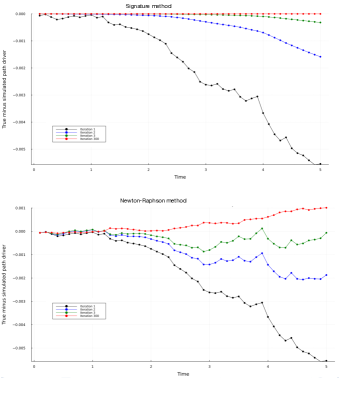
Figure 3. CIR model: approximation error for Newton-Raphson and signature methods, for $n=1,2,3,300$.

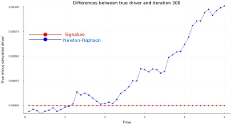
Figure 4. CIR model: approximation error for Newton-Raphson and signature methods, $n=300$.

4.2. Constant Elasticity of Variance model

We consider the system described by

(23) $$d\hat{Y}_{t}=\mu\hat{Y}_{t}dt+\sigma\hat{Y}_{t}^{\gamma}d\hat{X}_{t},$$

where $\hat{X}_{t}$ is a random piecewise linear path on partition ${\mathcal{D}}_{2}=\{k\delta,k=0,1,\dots,N\}$ of $[0,T]$, with $\delta=0.01$, $N=2000$ and $T=20$. We also set $\mu=0.05$, $\sigma=0.15$, $\gamma=1.5$ and $Y_{0}=1$. The piecewise linear path $\hat{X}$ is generated in the same way as in the CIR example but on partition ${\mathcal{D}}_{2}$. We apply methods 1 and 2, as described in subsection 4.1.

The results are displayed in figures 5 and 6. In figure 5, we plot $\hat{X}(n)-\hat{X}_{NR}(n)$ and $\hat{X}(n)-\hat{X}_{sig}(n)$ for $t\in[0,20]$ and $n=1,2,10,100$ and in figure 6, we show the same two errors for $n=300$. As in the CIR example, we see that the total error of the signature method is uniformly controlled while this is not the case for the Newton-Raphson method. Moreover, we see that the signature method converges much faster.

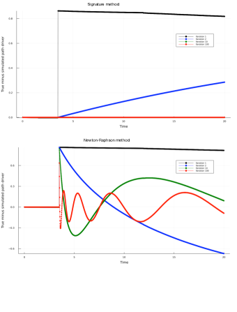
Figure 5. CEV model: approximation error for Newton-Raphson and signature methods, for $n=1,2,10,100$.

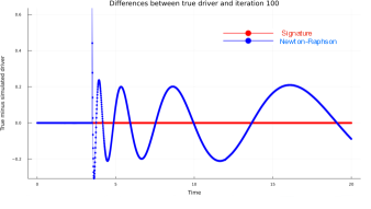
Figure 6. CEV model: approximation error for Newton-Raphson and signature methods, $n=100$.

References

- [1] I. Bailleul and J. Diehl. The Inverse Problem for Rough Controlled Differential Equations. SIAM J. Control Optim. 53(5): 2762–2780, 2015.
- [2] H. Boedihardjo, Xi Geng, T. Lyons, DanyuYang. The signature of a rough path: Uniqueness. it Advances in Mathematics: 293: 720-737, 2016.
- [3] L. Coutin and A Lejay. Sensitivity of rough differential equations: An approach through the Omega lemma. J. Differential Equations 264: 3899–3917, 2018.
- [4] P. Friz and N. Victoir. Multidimensional stochastic processes as rough paths: theory and applications, vol.120. CUP, 2010.
- [5] A. C. Hindmarsh, P. N. Brown, K. E. Grant, S. L. Lee, R. Serban, D. E. Shumaker and C. S. Woodward. SUNDIALS: Suite of nonlinear and differential/algebraic equation solvers. ACM Transactions on Mathematical Software (TOMS), 31(3): 363–396, 2005.
- [6] Y. Hu and D. Nualart. Parameter estimation for fractional Ornstein-Uhlenbeck processes, Statistics & Probability Letters, 80(11-12): 1030–1038, 2010.
- [7] W. G. Kelley and A. C. Peterson. The Theory of Differential Equations, (Second Edition), Springer, 2010.
- [8] P. Kidger, J Foster, Xuechen Li and T Lyons. Efficient and Accurate Gradients for Neural SDEs. NeurIPS, 2021b. arXiv:2105.13493
- [9] K. Kubilius and V. Skorniakov. On some estimators of the Hurst index of the solution of SDE driven by a fractional Brownian motion, Statistics & Probability Letters, 109:159–167, 2016.
- [10] Y. A. Kutoyants. Statistical inference for ergodic diffusion processes. Springer Science & Business Media, 2013.
- [11] T. Lyons and Z Qian. System Control and Rough Paths OUP, 2002.
- [12] A. Papavasiliou and K.B. Taylor. Approximate Likelihood Construction for Rough Differential Equations. arXiv:1612.02536
- [13] C. Rackauckas and Qing Nie. Differential equations .jl – a performant and feature-rich ecosystem for solving differential equations in julia. Journal of Open Research Software, 5(1), 2017.
- [14] Pu Zhang, Wei-Lin Xiao, Xi-Li Zhang, Pan-Qiang Niu. Parameter identification for fractional Ornstein-Uhlenbeck processes based on discrete observation. Economic Modelling 36: 198–203, 2014.