Multi-kink brane in Gauss-Bonnet gravity

Abstract

In this paper, we study the properties of thick branes generated by a bulk scalar field in the five-dimensional Einstein-Gauss-Bonnet Gravity. With the help of the superpotential method, we obtain a series of multi-kink brane solutions. We also analyze the linear stability of the brane system under tensor perturbations and prove that they are stable. The massless graviton is shown to be localized near the brane and hence the four-dimensional Newtonian potential can be recovered. By comparing the properties of these thick branes under different coupling parameters, we discuss the effect of the Gauss-Bonnet invariant on the thick branes.

1 Introduction

Among several interesting descriptions of our universe, an attractive one may be that our universe acts as a four-dimensional hypersurface called 3-brane embedded in higher-dimensional spacetime Akama:1982jy ; Rubakov:1983kea . Under such an assumption, gravity can propagate in the whole bulk since it is the dynamics of the spacetime itself. At low energy level, the Standard Model (SM) particles and interactions are trapped in the ordinary four-dimensional spacetime. In other words, the SM particles and fields can not propagate into extra dimensions and there is no confliction with the present four-dimensional experiments. While at high energy level, it would be possible for the SM particles to leave away from the four dimensions and propagate into extra dimensions. Therefore, studying the nature of higher-dimensional brane models could allow us to dig out some potential observational signatures of high-dimensional spacetime.

It is well known that Kaluza-Klein (KK) theory Kaluza:1921tu ; Klein:1991 is the first higher-dimensional theory that unifies Maxwell electromagnetism and Einstein gravity. It is described by a five-dimensional Riemannian geometry. Besides the unification of the Maxwell electromagnetism and Einstein gravity, KK theory still predicated the novel particles beyond the four-dimensional SM. These novel KK particles provide the possible rules to detect the extra dimensions. In 1982, Akama Akama:1982jy presented an early proposal of brane world. In this picture, we live in a dynamically localized 3-brane in a higher-dimensional spacetime. One year later, Rubakov and Shaposhnikov Rubakov:1983kea proposed a domain wall model in a higher-dimensional Minkowski spacetime. In this model, fermions can be trapped on the domain wall through the Yukawa coupling mechanism Rubakov:1983kea . With the development of higher-dimensional gravity theories, more and more works focused on the nature of extra dimensions Arkani:1998 ; Randall:1999 ; Randall2:1999 ; Hsin:2010 ; Rizzo:2010 ; Maartens:2010 ; Liu:2017gcn and various potential observable effects of extra dimensions were proposed. Especially at the end of the 20th century, the Arkani-Hamed-Dimopoulos-Dvali (ADD) model Arkani:1998 and the Randall-Sundrum (RS) model Randall:1999 provided a new way to solve the hierarchical problem in the SM of particle physics. This attracts the attention of physicists once again and opens a new era for studying extra dimensions.

In brane world scenarios, there are thin or thick branes in terms of their width along the extra dimensions. Both the branes are thin in ADD and RS models because the thickness of the brane has been neglected. Note that, in the thin brane model, the scalar curvature comes to be singular at the core of the brane because of the zero width Merab1998 . To deal with this singularity, the Israel-Lanczos junction condition Israel1966 should be introduced. Physically, a brane should have thickness and it emerges as an alternative to thin brane configuration. That is to say, a brane should have nontrivial width along extra dimensions and there is no singularity problem as appeared in the thin braneworld models. One way to obtain such nonsingular thick brane might be simply replacing the singular source term in the thin brane scenarios with a nonsingular source term. A usual source term is that of one or more scalar fields DeWolfe:1999cp ; Bronnikov:2003gg ; Bazeia:2008zx ; Toharia:2010ex ; Bazeia:2003aw ; Novikov:2015iph ; Bazeia:2015owa ; Xie:2021ayr ; Wan:2020smy . There were some models based on the nonminimal coupling between gravity and the scalar field Nozari:2009zr ; Liu:2012gv ; Guo:2011wr ; Cardoso:2006nh . Those nontrivial sources induced many new phenomena and abundant brane configurations. Furthermore, thick brane models Xu:2014jda ; Zhong:2015pta ; Gu:2016nyo ; Zhou:2017xaq ; Zhong:2017ffr ; Gu:2018lub ; Cui:2020fiz ; Chen:2020zzs ; Yu:2015wma ; Rosa:2022fhl ; Rosa:2021tei ; Wang:2019igp ; Dzhunushaliev:2019wvv ; Nozari:2019shm . and thin brane models Banerjee:2017lxi ; Elizalde:2018rmz ; Banerjee:2020uil were investigated in the modified gravity theories such as $f(R)$ gravity. Especially, some brane solutions with rich structure were obtained in Cui:2020fiz ; Chen:2020zzs .

When the spacetime dimension is higher than four, the Einstein-Hilbert action can be supplemented with higher order curvature corrections which do not generate three or higher order terms of equations of motion Lovelock:1971yv . The gravity theory including the Gauss-Bonnet (GB) invariant term is a theory that satisfies the above-mentioned property, where the GB invariant arises as a correction in string theory Wheeler:1985nh ; Boulware:1985wk ; Zwiebach:1985kea ; Gross:1986mw and is defined as follows

$${\cal R}_{\rm GB}=R^{ABCD}R_{ABCD}-4R^{AB}R_{AB}+R^{2}.$$ (1)

The letters $A,B,C,D$ in this paper are the indexes of the whole spacetime. In four-dimensional spacetime, the GB term is a topological term and acts as the boundary term that does not have influence on the classical field equations. When the spacetime dimension satisfies $D\geq 5$, the GB term is no longer topological invariant and its influence will exit Zwiebach:1985kea . Recently, the GB term was applied to the investigation of inflation after the GW170817 event Odintsov:2020sqy ; Oikonomou:2021kql ; Odintsov:2020xji ; Oikonomou:2020oil ; Elizalde:2020zcb , cosmology Chirkov:2021epn ; Odintsov:2021nim ; Shamir:2021ptw , as well as black hole physics Yerra:2022alz ; Li:2021wqa ; Chen:2018nbh ; Hu:2013cia . In addition, the entanglement wedge cross section was investigated in a five-dimensional AdS-Vaidya spacetime with GB corrections Li:2021rff . It is also interesting to consider branes in the GB gravity. Thin brane models in the GB gravity were discussed in Refs. Kim:2000ym ; Kim:2000pz ; Neupane:2001kd ; Meissner:2001xg ; Aoyanagi:2004zz . Besides the thin brane model, the thick brane models in the GB gravity with a bulk scalar field were widely investigated Odintsov:2021nim ; Corradini:2000sw ; Neupane:2000wt ; Andrianov:2013vqa ; German:2013sk ; Giovannini:2001ta ; Farakos:2006sr ; HerreraAguilar:2011jm ; Dias:2015gga , and the brane model in the GB gravity was also applied to cosmology Charmousis:2002rc ; Brown:2006mh ; abdesselam2002brane ; Alberghi:2005vq ; Nozari:2013hra ; Konya:2006wr ; Okada:2014eva ; Herrera:2010vv ; Fomin:2018typ ; Nojiri:2001ae ; Nojiri:2002hz ; Lidsey:2002zw ; Diaz:2020iwx . The domain wall solutions constructed by two scalar fields combining either in a kink-antikink or a trapping bag configuration were found in five-dimensional GB gravity with one warped extra-dimension Giovannini:2006rj . Note that there is only one defect for the domain walls with kink or antikink, when the multi kinks are considered, the gravitating multidefects can be obtained. It was originally investigated in Refs. Giovannini:2006ye ; Giovannini:2006sw . However, there were still few works focused on thick branes with inner structure in the GB gravity. Therefore, in this paper, we would like to construct multi-kink brane solution in the higher-dimensional GB gravity and study the possible effects of the GB term on the brane structure. We also analyze the linear stability of the system under tensor perturbation and the localization of gravity.

The paper is organized as follows. In Sec. 2, we introduce the method to solve the thick brane solutions in GB gravity. The system can be reduced to the first-order formulas by introducing a superpotential. In Sec. 3, we construct thick branes with some superpotentials and a polynomial warp factor, respectively, and study the influences of the GB term on the thick brane. In Sec. 4, the linear stability of the brane system under the tensor perturbations and localization of gravity are analysed. Finally, a brief summary is given in Sec. 5.

2 Brane model in GB gravity

In this section, we will introduce a new method to solve the thick brane in GB gravity. The brane model in $D$-dimensional GB gravity is described by the following action

$$S=\int d^{D}x\sqrt{-g}\left[\frac{R}{2\kappa}+\alpha{\cal R_{\rm GB}}+{\cal L}_{m}\right],$$ (2)

where $\kappa=8\pi G_{D}=M_{*}^{2-D}$ with $G_{D}$ the $D$-dimensional gravitational constant and $M_{*}$ the $D$-dimensional fundamental mass scale, and $\alpha$ is the GB coupling constant with mass dimension $D-4$. In this paper, we use the units $\kappa=c=\hbar=1$ and define a dimensionless GB coupling constant $\tilde{\alpha}=\alpha/M_{*}^{D-4}$. The Lagrangian density of the scalar field is given by

$${\cal L}_{m}=-\frac{1}{2}g^{AB}\partial_{A}\phi\partial_{B}\phi-V(\phi),$$ (3)

where $V(\phi)$ is the scalar potential. Varying the action (2) with the metric and scalar field respectively, we can get the equations of motion as follows

$$G_{AB}-2\alpha\kappa Q_{AB} = \kappa T_{AB},$$ (4)

$$g^{AB}\nabla_{A}\nabla_{B}\phi-\frac{\partial V(\phi)}{\partial\phi} = 0,$$ (5)

where $G_{AB}=R_{AB}-\frac{1}{2}Rg_{AB}$ is the Einstein tensor and

$$Q_{AB} =\frac{1}{2}g_{AB}{\cal R_{\rm GB}}-2RR_{AB}+4R_{AC}R^{C}{}_{B}$$

$$+4R_{ACBD}R^{CD}-2R_{ACDE}R_{B}^{~{}CDE}$$ (6)

is the Lanczos tensor Lovelock:1972vz . The energy-momentum tensor of the scalar field reads

$$T_{\text{AB}}=g_{AB}{\cal L}_{m}+\partial_{A}\phi\partial_{B}\phi.$$ (7)

In this paper, we focus on the flat thick brane with $Z_{2}$ symmetry in a five-dimensional spacetime ($D=5$). The metric is written as Randall2:1999

$$ds^{2}=e^{2A(y)}\eta_{\mu\nu}dx^{\mu}dx^{\nu}+d\,y^{2},$$ (8)

where the warp factor $A(y)$ is an even function of the extra dimensional coordinate $y$, $\eta_{\mu\nu}$ is the four-dimensional Minkowski metric. The ordinary four-dimensional coordinate indexes $\mu,\nu$ are from 0 to 3. The scalar curvature is

$$R=-4\left(5A^{\prime 2}+2A^{\prime\prime}\right),$$ (9)

where the prime denotes the derivative with respect to the extra dimensional coordinate $y$. The explicit equations of motion are

$$6\left(A^{\prime\prime}+2A^{\prime 2}\right)-48\alpha\kappa A^{\prime 2}\left(A^{\prime\prime}+A^{\prime 2}\right)+\kappa\left(\phi^{\prime 2}+2V\right)=0,$$ (10a)

$$12A^{\prime 2}-48\alpha\kappa A^{\prime 4}-\kappa\left(\phi^{\prime 2}-2V\right)=0,$$ (10b)

$$4A^{\prime}\phi^{\prime}+\phi^{\prime\prime}-\frac{\partial V}{\partial\phi}=0.$$ (10c)

It can be shown that there are only two independent equations in Eqs. (10a)-(10c) for the three functions $V(\phi)$, $\phi(y)$, and $A(y)$. The scalar potential $V(\phi)$ contains the contribution of the cosmological constant. In addation, the scalar field $\phi$ is assumed to be an odd function of the extra dimensional coordinate $y$ to localize the fermion zero mode on the brane Liu:2009ve .

To solve Eqs. (10a)-(10b), we introduce the so called superpotential used in supergravity to reduce the second-order field equations (10a)-(10b) to the first-order ones. Such method has been used successfully in Refs. Bazeia:2003cv ; Brito:2001hd ; Afonso:2006gi ; 1999Gravitational ; 2004Fake ; 1993GReGr ; Julia2000 . We first introduce a superpotential $W(\phi)$. The relation between the warp factor $A(y)$ and the superpotential $W(\phi)$ is given by

$$A^{\prime}(y)=-\frac{1}{3}\kappa W(\phi),$$ (11)

where the superpotential $W(\phi)$ should be an odd function of $\phi$ since $A(y)$ and $\phi(y)$ are assumed to be even and odd, respectively. From Eq. (11), we have

$$A^{\prime\prime}(y)=-\frac{1}{3}\kappa W_{\phi}\phi^{\prime}(y).$$ (12)

Substituting the above two  equations (11) and (12) into Eqs. (10a)-(10c), we have

$$\frac{4}{3}\kappa^{2}W^{2}-2\kappa W_{\phi}\phi^{\prime}+\frac{16}{9}\alpha\kappa^{4}W^{2}W_{\phi}\phi^{\prime}$$

$$-\frac{16}{27}\alpha\kappa^{5}W^{4}+\kappa\Big{(}\phi^{\prime 2}+2V\Big{)}=0,$$ (13)

$$\frac{4}{3}\kappa^{2}W^{2}-\frac{16}{27}\alpha\kappa^{5}W^{4}-\kappa\Big{(}\phi^{\prime 2}-2V\Big{)}=0,$$ (14)

$$\phi^{\prime\prime}-\frac{4}{3}\kappa W\phi^{\prime}-V_{\phi}=0,$$ (15)

where $W_{\phi}=\frac{dW(\phi)}{d\phi}$ and $V_{\phi}=\frac{dV(\phi)}{d\phi}$. After replacing the warp factor in terms of the relations (11) and (12), one can obtain a relation between the scalar field $\phi$ and the superpotential $W(\phi)$ by subtracting Eq. (2) from Eq. (14) as follows

$$\phi^{\prime}=\frac{1}{9}\left(9-8\alpha\kappa^{3}W^{2}\right)W_{\phi}.$$ (16)

One can further obtain the scalar potential by substituting Eq. (16) into Eq. (14):

$$V=\frac{1}{162}\left(W_{\phi}^{2}\big{(}9-8\alpha\kappa^{3}W^{2}\big{)}^{2}+12\kappa W^{2}\big{(}4\alpha\kappa^{3}W^{2}-9\big{)}\right).$$ (17)

In our thick brane model, the background scalar field has a kink-like configuration and it will approach to a constant $\phi_{\infty}$ when the extra dimensional coordinate $y\to\infty$. Thus the spacetime is an asymptotical AdS₅ spacetime, which is in accord with the RS brane model. The corresponding naked cosmological constant can be calculated from the scalar potential:

$$\Lambda_{5}=\lim_{y\rightarrow\infty}2\kappa V(\phi(y))=\lim_{\phi\rightarrow\phi_{\infty}}2\kappa V(\phi).$$ (18)

Now, the original field equations (10a)-(10c) have been replaced by the first-order formulas (11), (16), and (17). Once the superpotential $W(\phi)$ is given, we can solve all the functions for the brane solution with the help of the above first-order formulas.

In our setup, the scalar field $\phi(y)$ is an odd function of the extra dimensional coordinate $y$. Usually, it can not ensure that $\phi(y)$ is a monotonic function of $y$. However, we only consider the solution of a monotonic function $\phi(y)$ in this paper. Thus, for such a solution, it has an inverse function $y(\phi)$. This will help us to find solutions from given superpotentials conveniently. We can write the inverse function $y(\phi)$ from Eq. (16) as follows

$$y(\phi)=\int\frac{9}{\left(9-8\alpha\kappa^{3}W^{2}\right)W_{\phi}}\,d\phi.$$ (19)

The warp factor can also be obtained as

$${A}(y(\phi))=\int\frac{3\kappa W}{\left(8\alpha\kappa^{3}W^{2}-9\right)W_{\phi}}\,d\phi.$$ (20)

Furthermore, we introduce the conditions: $y(\phi=0)=0$ and $A(y=0)=0$. By specifying the suitable superpotential, one can obtain the thick brane solution from Eqs. (17), (19), and (20). The distribution of the thick brane can be described by the effective energy density along the extra dimension with respect to the static observer $u^{A}=(e^{A},0,0,0,0)$:

$$\rho=\tau_{MN}^{(\text{eff})}u^{M}u^{N}=-g^{00}\left(T_{00}+2\alpha Q_{00}\right),$$ (21)

where $\tau_{MN}^{(\text{eff})}=T_{MN}+2\alpha Q_{MN}$ is the effective energy-momentum tensor. It can also be expressed in terms of the superpotential as follows

$$\rho=\frac{1}{81}\left[W_{\phi}^{2}\left(9-8\alpha\kappa^{3}W^{2}\right)^{2}+6\kappa W^{2}\left(4\alpha\kappa^{3}W^{2}-9\right)\right].$$ (22)

Note that $\rho(|y|\rightarrow\infty)$ is nonvanishing since the above expression contains the contribution from the effective cosmological constant coming from the naked cosmological constant $\Lambda_{5}$ in (18) and the Lanczos tensor. In order to describe the shape of the brane better, we subtract the contribution of the effective cosmological constant, i.e., we make the following replacement

$$\rho(y)\rightarrow\rho(y)-\rho(|y|\rightarrow\infty).$$ (23)

Besides the superpotential method for solving thick brane system, one can also obtain the thick brane solutions by using the relations between the scalar field as well as scalar potential and the warp factor. This can be done conveniently with the following five-dimensional conformally flat metric

$$ds^{2}=e^{2A(z)}[\eta_{\mu\nu}dx^{\mu}dx^{\nu}+d\,z^{2}],$$ (24)

where the warp factor $e^{2A(z)}$ is a function of the extra dimensional coordinate $z$ and the relation between $z$ and $y$ is given by $e^{A}dz=dy$. With a known warp factor, one can derive the expressions for the scalar potential and scalar field:

$$V (\phi(z))=12\tilde{\alpha}M_{*}e^{-4A}\left(\partial_{z}A\right)^{2}\left[\left(\partial_{z}A\right)^{2}+\partial_{z}^{2}A\right]$$

$$~{}~{}~{}~{}~{}~{}~{}~{}~{}-\frac{3}{2}M_{*}^{3}e^{-2A}\left[3\left(\partial_{z}A\right)^{2}+\partial_{z}^{2}A\right],$$ (25)

$$\!\!\phi(z) \!=\!\int dz\sqrt{3M_{*}^{3}}\sqrt{\left[1-8\tilde{\alpha}\left(M_{*}^{-1}\partial_{z}e^{-A}\right)^{2}\right]\left[\left(\partial_{z}A\right)^{2}-\partial_{z}^{2}A\right]}.$$ (26)

Therefore, we can obtain the thick brane solution by directly specifying the form of the warp factor.

3 Brane solutions

In this section, we first consider various superpotentials for solving multi-kink branes. Then, we also construct a thick brane solution with a polynomial warp factor in the conformal coordinate. We will set $M_{*}=1$ in the numerical calculations or plots in this paper.

3.1 Solutions with superpotential method

Once a superpotential is given, the warp factor, the scalar field, the energy density, and the scalar potential can be obtained numerically, just as discussed in Sec. 2, and the property of the brane can be figured out. For some concrete examples, we consider following three types of superpotentials:

$$W_{1}(\phi)= M_{*}^{4}\left(a~{}\tilde{\phi}+b\,\tilde{\phi}~{}\text{sech}({\tilde{\phi}})\right),$$ (27)

$$W_{2}(\phi)= M_{*}^{4}\left(a~{}\tilde{\phi}+b\,\text{sinh}({\tilde{\phi}})\right),$$ (28)

$$W_{3}(\phi)= M_{*}^{4}\left(a~{}\tilde{\phi}+b\sin({\tilde{\phi}})\right),$$ (29)

where $\tilde{\phi}=\phi/(M_{*}^{3/2}v)$ is a dimensionless scalar field and $a$, $b$, and $v$ are dimensionless parameters. The first terms of the three superpotentials are the same, but the second ones have different asymptotic behaviors when the scalar field approaches infinity. We will show that multi-kink thick brane solutions can be obtained for all these superpotentials with different parameter spaces.

3.1.1 First superpotential

For the first superpotential (27), we obtain the scalar potential from (17), the function $y(\phi)$ from (19), and the warp factor from (20):

$$V(\phi)= \frac{2}{27}M_{*}^{5}\tilde{\phi}^{2}\big{(}b~{}\text{sech}({\tilde{\phi}})+a\big{)}^{2}$$

$$\times\left(4\tilde{\alpha}~{}\tilde{\phi}^{2}\big{(}b~{}\text{sech}({\tilde{\phi}})+a\big{)}^{2}-9\right)$$

$$+\frac{1}{162}M_{*}^{5}v^{-2}\left(9-8\tilde{\alpha}~{}\tilde{\phi}^{2}~{}\big{(}b~{}\text{sech}({\tilde{\phi}})+a\big{)}^{2}\right)^{2}$$

$$\times\Big{(}b~{}\text{sech}({\tilde{\phi}})\big{(}1-\tilde{\phi}~{}\tanh(\tilde{\phi})\big{)}+a\Big{)}^{2},$$ (30)

$$y(\phi)= M_{*}^{-1}\int_{0}^{\tilde{\phi}}\frac{9v^{2}}{b~{}\text{sech}(\tilde{\phi})-b~{}\tilde{\phi}~{}\tanh({\tilde{\phi}})~{}\text{sech}(\tilde{\phi})+a}$$

$$\times\frac{1}{9-8\tilde{\alpha}~{}(b~{}\tilde{\phi}~{}\text{sech}(\tilde{\phi})+a~{}\tilde{\phi})^{2}}d\tilde{\phi},$$ (31)

$$A(y(\phi))= \int_{0}^{\tilde{\phi}}\frac{3v^{2}\left(b~{}\tilde{\phi}~{}\text{sech}({\tilde{\phi}})+a~{}\tilde{\phi}\right)}{b~{}\text{sech}({\tilde{\phi}})-b~{}\tilde{\phi}~{}\tanh({\tilde{\phi}})~{}\text{sech}({\tilde{\phi}})+a}$$

$$\times\frac{1}{8~{}\tilde{\alpha}~{}\Big{(}b~{}\tilde{\phi}~{}\text{sech}({\tilde{\phi}})+a~{}\tilde{\phi}\Big{)}^{2}-9}d\tilde{\phi}.$$ (32)

Here, we also keep $M_{*}$ in these expressions in order to check the dimensions of the quantities. The energy density $\rho(y)$ can be obtained from Eqs. (21),  (22), and (23). We do not list it here.

The kink-like solution for the scalar field demands that the scalar field satisfies $\phi\rightarrow\text{const}=\phi_{\infty}$ when $y\rightarrow\infty$. That is to say, the integral function in Eq. (31) for $y(\phi)$ must approach to infinity when $\phi\rightarrow\phi_{\infty}$. Thus we get the constraints on the parameters $\tilde{\alpha}$, $a$, and $b$ that could support the existence of thick brane solutions. We list the constraints as follows

• when $\tilde{\alpha}>0$, the restriction is $a\neq-b$;

• when $\tilde{\alpha}\leq 0$ and $b\geq 0$, the restriction is $-b<a<0.2511b$;

• when $\tilde{\alpha}\leq 0$ and $b<0$, the restriction is $0.2511b<a<-b$.

Then, specifying the suitable values of parameters $a$ and $b$, we can obtain the single-kink, double-kink, and triple-kink thick brane solutions. See the corresponding results in Fig. 1 with the values of the parameters given in Table 1. In this subsection, we set $v=1$ for the scalar potential. From Fig. 1 we can see that the triple-kink scalar field configuration has a step-like energy density which is a new feature of the multi-kink scalar field.

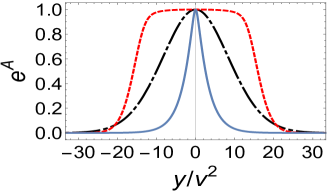
(a) Warp factor

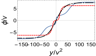
(b) Scalar field

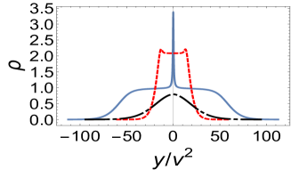
(c) Energy density

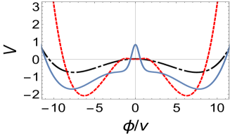
(d) Scalar potential

Figure 1: The brane solutions for the first superpotential (27). The black dot dashed lines, red dashed lines, and dark blue lines correspond to the single-kink, double-kink, and triple-kink scalar field solutions, respectively. The values of the parameters are listed in Table 1.

Table 1: Parameters used in Fig. 1

Lines	$\tilde{\alpha}$	$a$	$b$
Black dot dashed lines	0.500	0.200	0.010
Red dashed lines	0.180	0.400	-0.375
Dark blue lines	0.220	0.290	1.000

3.1.2 Second superpotential

Next, we use the second superpotential (28) to construct thick brane solutions. The corresponding expression of the scalar potential is

$$V(\phi)=\frac{2M_{*}^{5}}{27}\left(a\tilde{\phi}+b\sinh(\tilde{\phi})\right)^{2}\left(4\tilde{\alpha}\left(a\tilde{\phi}+b\sinh(\tilde{\phi})\right)^{2}-9\right)$$

$$+\frac{M_{*}^{5}}{162}v^{-2}\left(b\cosh(\tilde{\phi})+a\right)^{2}\left(9-8\tilde{\alpha}\left(a\tilde{\phi}+b\sinh(\tilde{\phi})\right)^{2}\right)^{2}.$$ (33)

Substituting the superpotential (28) into Eqs. (19),  (20), and (23), the function $y(\phi)$, the warp factor $A(y)$, and the energy density $\rho(y)$ can be obtained. We also need to restrict the parameters $\tilde{\alpha}$, $a$, and $b$ with Eq. (19) that could support the existence of thick brane solutions just like we did in Sec. 3.1.1. The result is

• when $\tilde{\alpha}>0$, the restriction is $b\neq-a$;

• when $\tilde{\alpha}\leq 0$, the restriction is $b^{2}<-ab$.

With this superpotential, we can also find thick brane solutions with single-kink and double-kink scalar field configurations. We show three different solutions with double-kink configurations in Fig. 2, for which the parameters are given in Table 2.

Table 2: Parameters used in Fig. 2

Lines	$\tilde{\alpha}$	$a$	$b$
Black dot dashed lines	-0.003	-10.0	0.050
Red dashed lines	-0.003	-11.0	0.050
Dark blue lines	0.0001	2.00	2.00

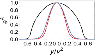
(a) Warp factor

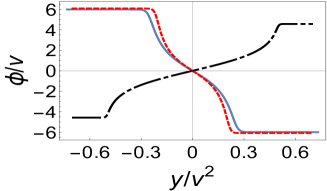
(b) Scalar field

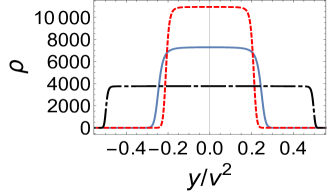
(c) Energy density

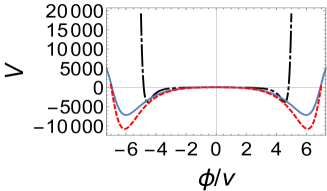
(d) Scalar potential

Figure 2: The brane solutions for the second superpotential (28). All three lines correspond to the double-kink solutions. The values of the parameters are listed in Table 2.

3.1.3 Third superpotential

At last, we use the third superpotential (29) to derive the thick brane solutions. With the above superpotential, we get the scalar potential as follows

$$V(\phi) =\frac{2M_{*}^{5}}{27}\big{(}a~{}\tilde{\phi}+b\sin(\tilde{\phi})\big{)}^{2}\big{(}4\tilde{\alpha}\big{(}a~{}\tilde{\phi}+b~{}\sin(\tilde{\phi})\big{)}^{2}-9\big{)}$$

$$+\frac{M_{*}^{5}}{162}v^{-2}(a+b\cos(\tilde{\phi}))^{2}\Big{(}9-8~{}\tilde{\alpha}(a~{}\tilde{\phi}+b\sin(\tilde{\phi}))^{2}\Big{)}^{2}.$$ (34)

Other functions can also be obtained with the above superpotential. For thick brane solutions, the constrains for the parameters that support the existence of thick brane solutions are

• when $\tilde{\alpha}>0$, then $a\neq\pm b$;

• when $\tilde{\alpha}\leq 0$, then $-b^{2}<ab<b^{2}$.

The superpotential (29) has rich structures due to the combination of the linear term $\tilde{\phi}$ and the periodic function $\sin(\tilde{\phi})$. For such superpotential, we find that any number of kinks for a background scalar field can be constructed with some suitable parameters. For instance, the number of kinks approaches to infinity when the parameters satisfy $a>-b>0$ and $\tilde{\alpha}\rightarrow+0$. This is a new result of the GB term and the superpotential (29). We show some multi-kink brane solutions in Fig. 3.

Table 3: Parameters used in Fig. 3

Lines	$\tilde{\alpha}$	$a$	$b$
Black dot dashed lines	0.065	0.700	-0.650
Red dashed lines	0.060	0.600	0.560
Dark blue lines	0.020	0.800	-0.720

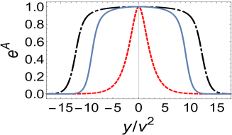
(a) Warp factor

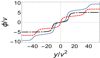
(b) Scalar field

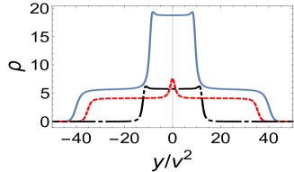
(c) Energy density

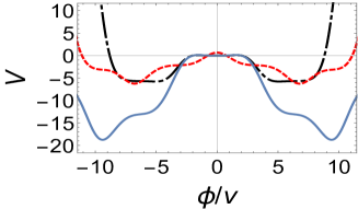
(d) Scalar potential

Figure 3: The brane solutions for the third superpotential (29). The black dot dashed lines, red dashed lines, and dark blue lines correspond to the double-kink, triple-kink, and 4-kink scalar field solutions, respectively. The values of the parameters are listed in Table 3.

Similarly, we can also find other brane world solutions for a given superpotential with our method given in the last section. This method is powerful in the GB brane model and can be generalized to brane models in other gravity theories.

From the above three typical examples of multi-kink brane solutions, we see that the warp factors with even kink solutions seem fatter than the ones with odd kink solutions. The energy densities and scalar potentials of multi-kink scalar fields are obviously different for different numbers of kinks. In these solutions we can not distinguish the number of kinks from the warp factor. This is because the influence of the multi-kink scalar field to the warp factor is too small. With some suitable superpotentials, the influence to the warp factor can be seen. We also find that the GB term plays an important role in finding multi-kink scalar field solutions. For the above three superpotentials, we do not find multi-kink brane solutions in general relativity, but with the GB term we can. So, in brane world scenario, the GB term could lead to richer brane structure, which is a new feature of GB gravity.

3.2 Solution with a polynomial expanded warp factor

In the last subsection, we have introduced the superpotential method to solve the thick brane system and shown that we can obtain the thick brane solutions with multi-kink background scalar fields by choosing some suitable superpotentials. In this subsection, we focus on the second method introduced in the end of Sec. 2. As an example, we adopt the following polynomial expanded warp factor with respect to the extra dimensional coordinate $z$:

$$e^{A(z)} =\sqrt{\frac{s_{1}(z)}{s_{2}(z)}},$$ (35)

$$s_{1}(z) =\sum_{i=0}^{n}(kz)^{2i},$$ (36)

$$s_{2}(z) =\sum_{i=0}^{n+1}(kz)^{2i},$$ (37)

where $n$ is a nonnegative integer and $k$ is a positive real parameter with mass dimension. The scalar potential and the scalar field can be solved from (25) and (26), respectively. It can be seen that $\tilde{\alpha}\leq\frac{1}{8}\frac{M_{*}^{2}}{k^{2}}$ can guarantee the scalar field is real. We plot the brane solutions in Fig. 4 and Fig. 5 by choosing different values of $n$ and $\tilde{\alpha}$, respectively. Since the warp factor and energy density are independent of $\tilde{\alpha}$, we do not repeat their plots in Fig. 5. With the increase of the parameter $n$, the warp factor shown in Fig. 4(a) becomes much wider with a platform around $z=0$, and the scalar field shown in Fig. 4(b) becomes double-kink from single-kink when $n\geq 1$. The energy density in Fig. 4(c) shows that the brane splits into two sub-branes. When the parameter $n$ increases to infinity, the warp factor, the scalar field, the energy density, and the scalar potential still have the similar shapes as the case of a finite $n$. From Fig. 5 we see that the scalar field and scalar potential are stretched with the decrease of the parameter $\tilde{\alpha}$.

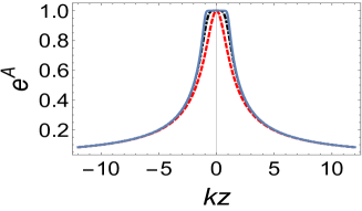
(a) Warp factor

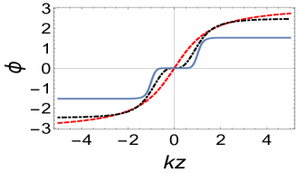
(b) Scalar field

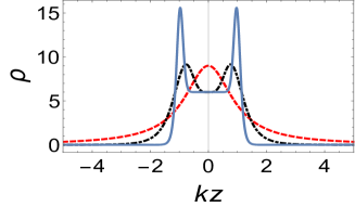
(c) Energy density

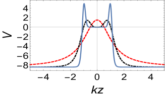
(d) Scalar potential

Figure 4: The brane solutions for the warp factor  (35) with different values of $n$. The red dashed lines, black dot dashed lines, and dark blue lines correspond to $n=0$, $n=2$, and $n=9$, respectively. Here we let $\tilde{\alpha}=-0.1$.

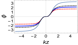
(a) Scalar field

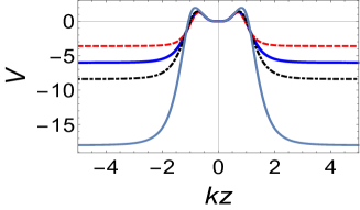
(b) Scalar potential

Figure 5: The brane solutions for the warp factor  (35) with different values of $\tilde{\alpha}$. The red dashed lines, blue solid lines, black dot dashed lines, and dark blue lines correspond to $\tilde{\alpha}=0.1$, $\tilde{\alpha}=0$, $\tilde{\alpha}=-0.1$, and $\tilde{\alpha}=-0.5$, respectively. Here we let $n=2$.

4 Stability of the system and localization of gravity

So far, we have obtained four kinds of thick brane solutions. In this section we study the linear stability of the brane system under tensor perturbations of the background metric. The total metric is given by

$$ds^{2}=e^{2A(z)}\big{[}(\eta_{\mu\nu}+h_{\mu\nu})dx^{\mu}dx^{\nu}+d\,z^{2}\big{]},$$ (38)

where $h_{\mu\nu}=h_{\mu\nu}(x^{\mu},z)$ is a transverse and traceless tensor perturbation of the background metric (24). The transverse and traceless gauge conditions are given by $\partial^{\mu}h_{\mu\nu}=0=h^{\mu}_{\mu}$.

The linear perturbation equation is

$$\delta G_{\mu}^{\nu}-\epsilon\delta Q_{\mu}^{\nu}=\kappa\delta T_{\mu}^{\nu},$$ (39)

where $\epsilon=2\alpha\kappa$. The above equation can be expanded as

$$\left(1+2\epsilon\bar{R}\right)\delta R_{\mu}^{\nu}-\frac{1}{2}\bar{R}h_{\mu}^{\nu}-2\epsilon\bigg{[}\frac{1}{4}{\cal\bar{R}_{\rm GB}}h_{\mu}^{\nu}$$

$$+2(\delta R_{\mu\beta}\bar{R}^{\nu\beta}+\bar{R}_{\mu\beta}\delta R^{\nu\beta})+2(\delta R_{AB}\bar{R}_{\mu}^{A\nu B}+\bar{R}_{AB}\delta R_{\mu}^{A\nu B})$$

$$-(\delta R_{\mu ABC}\bar{R}^{\nu ABC}+\bar{R}_{\mu ABC}\delta R^{\nu ABC})\bigg{]}=\kappa\delta T_{\mu}^{\nu}.$$ (40)

The quantities with a bar and with a delta in Eq. (40) correspond to the background and the perturbation, respectively. With the help of the equations of motion of the background, the equation for the tensor perturbation under the transverse and traceless gauges can be derived as follows Giovannini:2001ta

$$\left(1-4\epsilon e^{-2A}\partial_{z}^{2}A\right)\Box^{(4)}h_{\mu}^{\nu}+\left[1-4\epsilon e^{-2A}(\partial_{z}A)^{2}\right]\partial_{z}^{2}h_{\mu}^{\nu}$$

$$+\left[3\partial_{z}A-4\epsilon e^{-2A}\left(2(\partial_{z}A)\partial_{z}^{2}A+(\partial_{z}A)^{3}\right)\right]\partial_{z}h_{\mu}^{\nu}=0,$$ (41)

where $\Box^{(4)}=\eta^{\mu\nu}\partial_{\mu}\partial_{\nu}$ denotes the four-dimensional d’Alembert operator on the brane. The above equation can also be given in the physical coordinate $y$ by the coordinate transformation $dy=e^{A}dz$. The result is

$$\square^{(4)}h_{\mu}^{\nu}+F^{2}(y)h_{\mu}^{\nu}{{}^{\prime\prime}}+H(y)h_{\mu}^{\nu}{{}^{\prime}}=0,$$ (42)

where the prime denotes the derivative respect to physical coordinate $y$ and

$$F(y) =e^{A}\sqrt{\frac{\left(1-4\epsilon A^{\prime 2}\right)}{1-4\epsilon(A^{\prime 2}+A^{\prime\prime})}},$$ (43)

$$H(y) =e^{2A}\frac{4(A^{\prime}-2\epsilon A^{\prime}A^{\prime\prime}-4\epsilon A^{\prime 3})}{1-4\epsilon(A^{\prime 2}+A^{\prime\prime})}.$$ (44)

Then, by considering the KK decomposition of the tensor perturbation $h_{\mu}^{\nu}(x^{\mu},y)=\chi_{\mu}^{\nu}(x^{\mu})\varphi(y)$, we obtain the four-dimensional Klein-Gordon equation of the four-dimensional KK graviton $\chi_{\mu}^{\nu}(x^{\mu})$ with mass $m$ and the equation of the extra-dimensional part $\varphi(y)$:

$$\left(\Box^{(4)}-m^{2}\right)\chi_{\mu}^{\nu}(x^{\mu}) =0,$$ (45)

$$F^{2}(y)\varphi^{\prime\prime}(y)+H(y)\varphi^{\prime}(y)+m^{2}\varphi(y) =0.$$ (46)

Using another coordinate transformation $dy=F(y(w))dw$, equation (46) can be rewritten in the coordinate $w$ as

$$\partial_{w}^{2}\varphi(w)+\mathcal{K}(w)\partial_{w}\varphi(w)+m^{2}\varphi(w)=0,$$ (47)

where $\mathcal{K}(w)=\frac{H-\partial_{w}F}{F}$. Finally, by making the field transformation $\varphi(w)=f(w)\xi(w)$ with the function $f(w)$ satisfying

$$\frac{\partial_{w}f(w)}{f(w)}=\frac{1}{2}\left(\frac{\partial_{w}F(w)}{F(w)}-\frac{H(w)}{F(w)}\right),$$ (48)

we can transform the equation for $\varphi(w)$ as the following Schrödinger-like equation

$$\left(-\partial_{w}^{2}+V_{\text{eff}}(w)\right)\xi(w)=m^{2}\xi(w),$$ (49)

where the effective potential in the coordinate $w$ is given by

$$V_{\text{eff}}(w)=\frac{2F\left(\partial_{w}H-\partial_{w}^{2}F\right)-4H\partial_{w}F+3(\partial_{w}F)^{2}+H^{2}}{4F^{2}}.$$ (50)

The Schrödinger-like equation (49) can be expressed as the following form

$$Q^{\dagger}Q\xi(w)=m^{2}\xi(w),$$ (51)

where the operators $Q$ and $Q^{\dagger}$ are given by

$$Q=\partial_{w}+P(w),~{}~{}~{}~{}Q^{\dagger}=-\partial_{w}+P(w),$$ (52)

$$P(w)=\frac{1}{2}\left[\frac{\partial_{w}F}{F}-\frac{H}{F}\right].$$ (53)

Equation (51) guarantees $m^{2}\geq 0$ and there is no tachyonic graviton. So it is proved that the system is stable under the linear tensor perturbations. The tensor zero mode can be obtained by solving Eq. (51) with $m^{2}=0$:

$$\xi_{0}(w)=N_{0}e^{\pm\int{P(w)dw}},$$ (54)

where $N_{0}$ is the normalization constant. A localized graviton zero mode should satisfy the normalization condition $\int_{-\infty}^{\infty}\xi_{0}^{2}(w)dw=1$.

Next, we use the relation $\frac{\partial w}{\partial y}=\frac{1}{F}$ to write the expressions of the effective potential $V_{\text{eff}}$ and the tensor zero mode $\xi_{0}$ in the physical coordinate $y$:

$$V_{\text{eff}}(w(y)) =\frac{1}{4}\left(\frac{H^{2}(y)}{F^{2}(y)}-\frac{4H(y)F^{\prime}(y)}{F(y)}+F^{\prime 2}(y)\right)$$

$$+\frac{1}{4}\Big{(}2H^{\prime}(y)-2F(y)F^{\prime\prime}(y)\Big{)},$$ (55)

$$\xi_{0}(w(y)) =N_{0}e^{\int{\mathcal{P}_{\pm}(y)dy}},$$ (56)

where the functions $\mathcal{P}_{\pm}(y)$ are given by

$$\mathcal{P}_{\pm}(y)=\pm\frac{F(y)F^{\prime}(y)-H(y)}{2F(y)^{2}}.$$ (57)

For an asymptotic AdS₅ spacetime described by the metric (8), the warp factor $e^{A(y)}$ tends to $A(y)\rightarrow-k|y|$ when $|y|\rightarrow\infty$. Thus, the behavior of the effective potential at infinity is

$$\lim_{|y|\rightarrow\infty}V_{\text{eff}}\rightarrow\frac{15}{4}k^{2}e^{-2k|y|},$$ (58)

which shows that it will tend to zero when $|y|\rightarrow\infty$. The asymptotic behavior of the factor $\int\mathcal{P}_{\pm}dy$ of the zero mode at infinity is

$$\lim_{|y|\rightarrow\infty}\int{\mathcal{P}_{\pm}(y)dy}=\pm\left(\frac{3k}{2}|y|+C_{0}\right),$$ (59)

where $C_{0}$ is an integration constant. The asymptotic behavior (59) shows that the following condition

$$\int_{-\infty}^{\infty}\xi_{0}(y)^{2}dy=1$$ (60)

can be satisfied with a finite normalization constant $N_{0}$ for the case of $\mathcal{P}_{-}$ in the expression (59). Therefore, it is proved that the corresponding zero mode $\xi_{0}(w(y))=N_{0}e^{\int{\mathcal{P}_{-}(y)dy}}$ is localized on the brane and the four-dimensional Newtonian potential can be recovered.

Next, we focus on the profiles of the effective potentials and the corresponding configurations of the tensor zero modes on the thick brane solutions obtained in Sec. 3.

Note that, the effective potential (4) would diverge when the function $F(y)$ given in Eq. (43) goes to zero or the function $H(y)$ given in Eq. (44) diverges at certain finite extra dimension coordinate $y=y_{0}$, which is equivalent to

$$\left(4\epsilon A^{\prime 2}-1\right)\left(4\epsilon\left(A^{\prime 2}+A^{\prime\prime}\right)-1\right)=0.$$ (61)

The divergence of the effective potential means that there exists a nonsmooth tensor zero mode in the smooth thick brane.

Finally, we give the shapes of the effective potentials and tensor zero modes of our four kinds of thick brane solutions. Figures 6, 7, and 8 show the effective potentials and tensor zero modes of the thick brane solutions generated by the superpotentials (27), (28), and (29), respectively. It can be seen that the distribution of each effective potential is consistent with the energy density of the corresponding thick brane. With the specific superpotential $W(\phi)$, the effective potential $V_{\text{eff}}$ can have a richer structure. For instance, in Fig. 7 one can see that there are several wells in the effective potential. Figures 9 and 10 show the effective potential and tensor zero mode of the thick brane solution (35) for different values of $n$ and $\tilde{\alpha}$, respectively. Here, we obtain the discontinuous effective potential and nonsmooth tensor zero mode for a smooth thick brane when $n$ or $-\tilde{\alpha}$ has a large value. This is a new feature that did not find in general relativity. Although the profiles of these effective potentials and tensor zero modes are quite different, the localization condition (60) are satisfied and so all the zero modes we obtained can be localized on the brane and the four-dimensional Newtonian potential can be recovered.

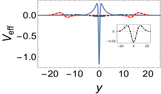
(a) Effective potential

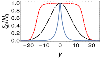
(b) Zero mode

Figure 6: The effective potential and zero mode for the first brane solution given in Sec. 3.1 with the superpotential (27). The parameters are given in Table 1.

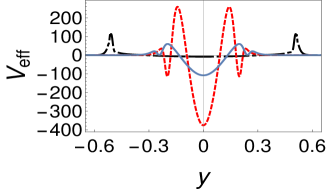
(a) Effective potential

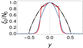
(b) Zero mode

Figure 7: The effective potential and zero mode for the second brane solution in Sec. 3.1 with the superpotential (28). The parameters are given in Table 2.

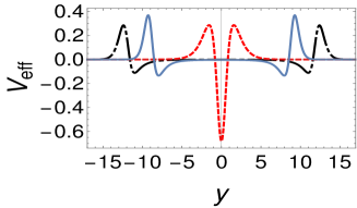
(a) Effective potential

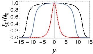
(b) Zero mode

Figure 8: The effective potential and zero mode for the third brane solution in Sec. 3.1 with the superpotential (29). The parameters are given in Table 3.

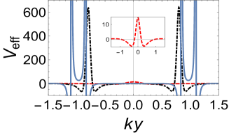
(a) Effective potential

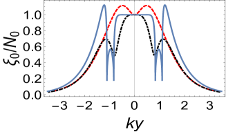
(b) Zero mode

Figure 9: The effective potential and zero mode for the brane solution given in Sec. 3.2 with the given warp factor (35) for different values of $n$. The parameters are set to $\tilde{\alpha}=-0.1$ and $n=(0,2,9)$ for the red dashed, black dot dashed, and dark blue lines, respectively.

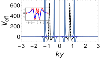
(a) Effective potential

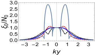
(b) Zero mode

Figure 10: The effective potential and zero mode for the brane solution given in Sec. 3.2 with the given warp factor (35) for different values of $\tilde{\alpha}$. The parameters are set to $n=2$ and $\tilde{\alpha}=(0.1,0,-0.1,-0.5)$ for the red dashed, black dot dashed, and dark blue lines, respectively.

5 Conclusions

It is well known that the GB term is a topological invariant and does not affect the equations of motion in four-dimensional spacetime. However, when the spacetime dimension satisfies $D\geq 5$, the GB term is no longer a topological invariant and its influence should be considered. Thus, in this paper we investigated the property of a thick brane in the five-dimensional Einstein GB gravity and showed that how the GB term affects the property of a thick brane. We introduced two methods for solving the thick brane solution. In the first method, all the variables including the warp factor $A$, the scalar potential $V$, and the extra dimensional coordinate $y$ are viewed as functions of the scalar field $\phi$. Then we can write the brane solution formally under the help of an auxiliary superpotential $W(\phi)$, which is given by Eqs. (17), (19), and (20). Note that, in this method, we have an assumption, i.e., the scalar field $\phi(y)$ is a monotonic function of the extra dimensional coordinate $y$. It was shown that this novel method works well for solving thick brane solutions with various superpotentials. In the second method, the expressions for the scalar field and scalar potential were obtained in terms of the warp factor, and one can directly obtain the thick brane solution by specifying a warp factor.

By choosing three special kinds of superpotentials, we first derived three types of thick brane solutions. We gave the constraints for the parameters in the superpotentials (27), (28), and (29) that could support the existence of a thick brane solution. We showed that one can construct multi-kink thick brane solutions with a suitable superpotential. We then obtained the thick brane solution by specifying a polynomial expanded warp factor.

All the thick brane solutions are linearly stable under tensor perturbations, and the corresponding tensor zero modes can be localized on the thick branes and the four-dimensional Newtonian potential can be recovered. The effective potentials in these brane models for the KK gravitons have a rich structure such as multi-well, which would lead to massive resonant KK gravitons Guo:2011wr ; Xu:2014jda ; Chen:2020zzs ; Yu:2015wma . Furthermore, it was found that one can obtain a discontinuous effective potential and nonsmooth tensor zero mode in the smooth thick brane solution, which was not found in general relativity. This singularity is originated from the zero pint of the function $F(y)$ (43) or the divergence of the function $H(y)$ given in Eq. (44) in the effective potential (50). The singularity condition is given by Eq. (61), from which it is clear that this singularity comes from the GB term for some parameter space and there is no singularity in general relativity. Such situation was also found in the $f(R)$ brane model, see Ref. Xu:2014jda for the details. The inner structure of the effective potential with singularities will also support a series of resonant KK gravitons. We will investigate these issues in the future work.

6 Acknowledgements

This work was supported in part by the National Key Research and Development Program of China (Grant No. 2020YFC2201503), the National Natural Science Foundation of China (Grants No. 11875151, No. 12105126, and No. 12047501), the China Postdoctoral Science Foundation (Grant No. 2021M701531), the 111 Project (Grant No. B20063), and the Fundamental Research Funds for the Central Universities (Grant No. lzujbky-2020-it04, No. lzujbky-2021-pd08). Y.X. Liu was supported by Lanzhou City’s scientific research funding subsidy to Lanzhou University.

References

- (1) K. Akama, An Early Proposal of ‘Brane World’, Lect. Notes Phys. 176 (1982) 267, [arXiv:hep-th/0001113].
- (2) V. A. Rubakov and M. E. Shaposhnikov, Do we live inside a domain wall?, Phys. Lett. B 125 (1983) 136.
- (3) Th. Kaluza, Zum Unitätsproblem der Physik, Int. J. Mod. Phys. D 27 (2018) 1870001, [arXiv:1004.3962[hep-th]].
- (4) O. Klein, Quantum theory and 5-dimensional relativity theory, Z. Phys. 37 (1926) 895.
- (5) N. Arkani-Hamed, S. Dimopoulos, and G. R. Dvali, The hierarchy problem and new dimensions at a millimeter, Phys. Lett. B 429 (1998) 263, [arXiv:hep-ph/9803315].
- (6) L. Randall and R. Sundrum, A Large mass hierarchy from a small extra dimension, Phys. Rev. Lett. 83 (1999) 17, [arXiv:hep-ph/9905221].
- (7) L. Randall and R. Sundrum, An alternative to compactification, Phys. Rev. Lett. 83 (1999) 4690, [arXiv:hep-th/9906064].
- (8) H. C. Cheng, Theoretical Advanced Study Institute in Elementary Particle Physics: Physics of the Large and the Small, (2011) 125-162, [arXiv:1003.1162[hep-ph]].
- (9) T. G. Rizzo, Introduction to Extra Dimensions, AIP Conf. Proc. 1256 (2010) 27, [arXiv:1003.1698[hep-ph]].
- (10) Y. X. Liu, Introduction to Extra Dimensions and Thick Braneworlds, Memorial Volume for Yi-Shi Duan, pp. 211-275 (2018), [arXiv:1707.08541[hep-ph]].
- (11) R. Maartens and K. Koyama, Brane-World Gravity, Living Rev. Rel. 13 (2010) 5, [arXiv:1004.3962[hep-th]].
- (12) M. Gogberashvili, Hierarchy problem in the shell-Universe model, Int. J. Mod. Phys. D 11 (2002) 1635, [arXiv:hep-ph/9812296].
- (13) W. Israel, Singular hypersurfaces and thin shells in general relativity, Nuovo Cim. B 44 (1966) 1.
- (14) O. DeWolfe, D. Z. Freedman, S. S. Gubser, and A. Karch, Modeling the fifth-dimension with scalars and gravity, Phys. Rev. D 62 (2000) 046008, [arXiv:hep-th/9909134].
- (15) K. A. Bronnikov and B. E. Meierovich, A General thick brane supported by a scalar field, Grav. Cosmol. 9 (2003) 313, [arXiv:gr-qc/0402030].
- (16) D. Bazeia, A. R. Gomes, L. Losano, and R. Menezes, Braneworld Models of Scalar Fields with Generalized Dynamics, Phys. Lett. B 671 (2009) 402, [arXiv:0808.1815[hep-th]].
- (17) M. Toharia, M. Trodden, and E. J. West, Scalar Kinks in Warped Extra Dimensions, Phys. Lett. D 82 (2010) 025009, [arXiv:1002.0011[hep-ph]].
- (18) D. Bazeia, C. Furtado, and A. R. Gomes, Brane structure from scalar field in warped space-time, JCAP 02 (2004) 002, [arXiv:hep-th/0308034].
- (19) Oleg O. Novikov, A. A. Andrianov, and V. A. Andrianov, Thick branes from self-gravitating scalar fields, AIP Conf. Proc. 1606 (2015) 313.
- (20) D. Bazeia, A. S. Lobão Jr, and R. Menezes, Thick brane models in generalized theories of gravity, Phys. Lett. B 743 (2015) 98, [arXiv:hep-th/1502.04757].
- (21) Q. Y. Xie, Q. M. Fu, T. T. Sui, L. Zhao, and Y. Zhong, First-order formalism and thick branes in mimetic gravity, Symmetry 13 (13) (2021) 1345, [arXiv:gr-qc/2102.10251].
- (22) J. J. Wan, Z. Q. Cui, W. B. Feng, and Y. X. Liu, Smooth braneworld in -dimensional asymptotically AdS spacetime, JHEP 05 (2021) 017, [arXiv:hep-th/2010.05016].
- (23) K. Nozari and S. D. Sadatian, Bouncing Universe with a Nonminimally Coupled Scalar Field on a Moving Domain Wall, Phys. Lett. B 676 (2009) 1, [arXiv:0904.4029[gr-qc]].
- (24) Y. X. Liu, F. W. Chen, H. Guo, and X. N. Zhou, Non-minimal Coupling Branes, JHEP 05 (2012) 108, [arXiv:1205.0210 [hep-th]].
- (25) H. Guo, Y. X. Liu, Z. H. Zhao, and F. W. Chen, Thick branes with a non-minimally coupled bulk-scalar field, Phys. Rev. D 85 (2012) 124033, [arXiv:1106.5216 [hep-th]].
- (26) C. Antonio, K. Koyama, A. Mennim, S. S. Seahra, and D. Wands, Coupled bulk and brane fields about a de Sitter brane, Phys. Rev. D 75 (2007) 084002, [arXiv:hep-th/0612202].
- (27) Z. G. Xu, Y. Zhong, H. Yu, and Y. X. Liu, The structure of -brane model, Eur. Phys. J. C. 75 (2015) 368, [arXiv:1405.6277[hep-th]].
- (28) Y. Zhong and Y. X. Liu, Pure geometric thick -branes: stability and localization of gravity, Eur. Phys. J. C. 76 (2016) 321, [arXiv:1507.00630[hep-th]].
- (29) B. M. Gu, Y. P. Zhang, H. Yu, and Y. X. Liu, Full linear perturbations and localization of gravity on brane, Eur. Phys. J. C. 77 (2017) 115, [arXiv:1606.07169[hep-th]].
- (30) X. N. Zhou, Y. Z. Du, H. Yu, and Y. X. Liu, Localization of Gravitino Field on Thick Branes, Sci. China Phys. Mech. Astron. 61 (2018) 110411, [arXiv:1703.10805[hep-th]].
- (31) Y. Zhong, K. Yang, Ke, and Y. X. Liu, Linearization of a warped theory in the higher-order frame II: the Equation of motion approach, Phys. Rev. D 97 (2018) 044032, [arXiv:1708.03737 [gr-qc]].
- (32) B. M. Gu, Y. X. Liu, and Y. Zhong, Stable Palatini braneworld, Phys. Rev. D 98 (2018) 024027, [arXiv:1804.00271[hep-th]].
- (33) Z. Q. Cui, Z. C. Lin, J. J. Wan, Y. X. Liu, and L. Zhao, Tensor Perturbations and Thick Branes in Higher-dimensional Gravity, JHEP 12 (2020) 130, [arXiv:2009.00512[hep-th]].
- (34) J. Chen, W. D. Guo, and Y. X. Liu, Thick branes with inner structure in mimetic f(R) gravity, Eur. Phys. J. C 81 (2021) 709, [arXiv:2011.03927[gr-qc]].
- (35) H. Yu, Y. Zhong, B. M. Gu, and Y. X. Liu, Gravitational resonances on -brane, Eur. Phys. J. C 76 (2016) 195, [arXiv:1506.06458[gr-qc]].
- (36) J.L. Rosa, A.S. Lobão, D. Bazeia, Impact of compactlike and asymmetric configurations of thick branes on the scalar–tensor representation of gravity, Eur. Phys. J. C 82 (3) (2022) 191, [arXiv:2202.10713[gr-qc]].
- (37) J.L. Rosa, M.A. Marques, D. Bazeia, S.N. Lobo, Thick branes in the scalar–tensor representation of f(R, T) gravity, Eur. Phys. J. C 81 (11) (2021) 981, [arXiv:2105.06101[gr-qc]].
- (38) L.L. Wang, H. Guo, C.E. Fu, Q.Y. Xie, Gravity and Matters on a pure geometric thick polynomial brane, Eur. Phys. J. C 82 (3) (2019) 191, [arXiv:1912.01396[hep-th]].
- (39) V. Dzhunushaliev, V. Folomeev, G. Nurtayeva, S.D. Odintsov, Thick branes in higher-dimensional gravity, Int. J. Geom. Meth. Mod. Phys. 17 (3) (2020) 2050036, [arXiv:1908.01312[gr-qc]].
- (40) K. Nozari, N. Sadeghnezhad, Braneworld mimetic gravity, Int. J. Geom. Meth. Mod. Phys. 16 (3) (2019) 1950042, [arXiv:1908.01312[gr-qc]].
- (41) N.Banerjee, T. Paul, Inflationary scenario from higher curvature warped spacetime, Eur. Phys. J. C 77 (10) (2017) 672, [arXiv:1706.05964[hep-th]].
- (42) E. Elizalde, S.D. Odintsov, T. Paul, D. Sáez-Chillón Gómez, Inflationary universe in gravity with antisymmetric tensor fields and their suppression during its evolution, Phys. Rev. D 99 (6) (2019) 063506, [arXiv:1811.02960[gr-qc]].
- (43) I. Banerjee, T. Paul, S. SenGupta, Bouncing cosmology in a curved braneworld, JCAP 02 (2021) 041, [2011.11886[gr-qc]].
- (44) D. Lovelock, The Einstein tensor and its generalizations, J. Math. Phys. 12 (1971) 498.
- (45) J. T. Wheeler, Symmetric Solutions to the Gauss-Bonnet Extended Einstein Equations, Nucl. Phys. B 268 (1986) 737.
- (46) D. G. Boulware and S. Deser, String Generated Gravity Models, Phys. Rev. Lett. 55 (1985) 2656.
- (47) B. Zwiebach, Curvature squared terms and string theories, Phys. Lett. B 156 (1985) 315.
- (48) D. J. Gross and J. H. Sloan, The Quartic Effective Action for the Heterotic String, Nucl. Phys. B 291 (1987) 41.
- (49) S. D. Odintsov, V. K. Oikonomou, and F. P. Fronimos, Rectifying Einstein-Gauss-Bonnet Inflation in View of GW170817, Nucl. Phys. B 958 (2020) 115135, [arXiv:2003.13724 [gr-qc]].
- (50) V. K. Oikonomou, A refined Einstein–Gauss–Bonnet inflationary theoretical framework, Class. Quant. Grav. 38 (19) (2021) 195025, [arXiv:2108.10460[gr-qc]].
- (51) S. D. Odintsov, V. K. Oikonomou, and F. P. Fronimos, Non-minimally coupled Einstein–Gauss–Bonnet inflation phenomenology in view of GW170817, Annals Phys. 420 (2020) 168250, [arXiv:2007.02309[gr-qc]].
- (52) V. K. Oikonomou and F. P. Fronimos, A Nearly Massless Graviton in Einstein-Gauss-Bonnet Inflation with Linear Coupling Implies Constant-roll for the Scalar Field, EPL 131 (3) (2020) 30001, [arXiv:2007.11915[gr-qc]].
- (53) E. Elizalde, S.D. Odintsov, V.K. Oikonomou, T. Paul, Extended matter bounce scenario in ghost free gravity compatible with GW170817, Nucl. Phys. B 954 (2020) 114984, [arXiv:2003.04264[gr-qc]].
- (54) D. Chirkov, S.A. Pavluchenko, Some aspects of the cosmological dynamics in Einstein–Gauss–Bonnet gravity, Mod. Phys. Lett. A 36 (13) (2021) 2150092, [arXiv:2101.12066[gr-qc]].
- (55) S. D. Odintsov, V. K. Oikonomou, and F. P. Fronimos, Late-time cosmology of scalar-coupled gravity, Class. Quant. Grav. 38 (7) (2021) 075009, [arXiv:2102.02239[gr-qc]].
- (56) M.F. Shamir, Bouncing universe in f(G,T) gravity, Phys. Dark Univ.32 (2021) 100794.
- (57) P.K. Yerra, C. Bhamidipati, Topology of black hole thermodynamics in Gauss-Bonnet gravity (2022), [arXiv:2202.10288[gr-qc]].
- (58) G.Q. Li, J.X. Mo, Y.W. Zhuang, Corrections to Hawking radiation and Bekenstein-Hawking entropy of novel four-dimensional black holes in Gauss- Bonnet gravity, Gen. Rel. Grav. 11 (2021) 107.
- (59) B. Chen, P.C. Li, Y. Tian, C.Y. Zhang, Holographic Turbulence in Einstein-Gauss-Bonnet Gravity at Large , JHEP 01 (2019) 156, [arXiv:hep-th/1804.05182].
- (60) C. Hu, X.X. Zeng and X.M. Liu, Phase transition and critical phenomenon of AdS black holes in Einstein-Gauss-Bonnet gravity, Sci. China Phys. Mech. Astron. 56 (2013) 1652-1663.
- (61) Y.Z. Li, C.Y. Zhang, X.M. Kuang, Entanglement wedge cross-section with Gauss-Bonnet corrections and thermal quench, Sci. China Phys. Mech. Astron. 64 (12) (2021) 120413, [arXiv:2102.12171[hep-th]].
- (62) J. E. Kim and H. M. Lee, Gravity in the Einstein-Gauss-Bonnet theory with the Randall-Sundrum background, Nucl. Phys. B 602 (2001) 346, [arXiv:0010093[hep-th]].
- (63) J. E. Kim, B. Kyae, and H. M. Lee, Various modified solutions of the Randall-Sundrum model with the Gauss-Bonnet interaction, Nucl. Phys. B 582 (2000) 296, [arXiv:hep-th/0004005].
- (64) I. P. Neupane, Completely localized gravity with higher curvature terms, Class. Quant. Grav. 19 (2002) 5507, [arXiv:hep-th/0106100].
- (65) K. A. Meissner and M. Olechowski, Brane localization of gravity in higher derivative theory, Phys. Rev. D 65 (2002) 064017, [arXiv:hep-th/0106203].
- (66) K. Aoyanagi and K. Maeda, Creation of a Brane World with Gauss-Bonnet Term, Phys. Rev. D 70 (2004) 123506, [arXiv:hep-th/0408008].
- (67) O. Corradini and Z. Kakushadze, Localized gravity and higher curvature terms, Phys. Lett. B 494 (2000) 302, [arXiv:hep-th/0009022].
- (68) I. P. Neupane, Consistency of higher derivative gravity in the brane background, JHEP 09 (2000) 040, [arXiv:hep-th/0008190].
- (69) A. A. Andrianov, V. A. Andrianov, and O. O. Novikov, Gravity effects on thick brane formation from scalar field dynamics, Eur. Phys. J. C 73 (2013) 2675, [arXiv:1306.0723[hep-th]].
- (70) G. German, H. A. Alfredo, M. Morejon, Dagoberto, Q. Israel, and R. Roldao, Study of field fluctuations and their localization in a thick braneworld generated by gravity nonminimally coupled to a scalar field with the Gauss-Bonnet term, Phys. Rev. D 98 (2014) 026004, [arXiv:1301.6444 [hep-th]].
- (71) M. Giovannini, Thick branes and Gauss-Bonnet self-interactions, Phys. Rev. D 64 (2001) 124004, [arXiv:hep-th/0107233].
- (72) K. Farakos and P. Pasipoularides, Gauss-Bonnet gravity, brane world models, and non-minimal coupling, Phys. Rev. D 75 (2007) 024018, [arXiv:hep-th/0610010].
- (73) H. A. Alfredo, M. M. Dagoberto, R. M. L. Refugio and I. Quiros, Thick braneworlds generated by a non-minimally coupled scalar field and a Gauss-Bonnet term: conditions for localization of gravity, Class. Quant. Grav. 29 (2012) 035012, [arXiv:1105.5479[hep-th]].
- (74) M. Dias, J. M. Hoff da Silva and R. da Rocha, Thick Braneworlds and the Gibbons-Kallosh-Linde No-go Theorem in the Gauss-Bonnet Framework, EPL 110 (2) (2015) 20004, [arXiv:1504.04243[gr-qc]].
- (75) C. Charmousis and J. F. Dufaux, General Gauss-Bonnet brane cosmology, Class. Quant. Grav. 19 (2002) 4671, [arXiv:hep-th/0202107].
- (76) R. A. Brown, Brane universes with Gauss-Bonnet-induced-gravity, Gen. Rel. Grav. 39 (2007) 477, [arXiv:gr-qc/0602050].
- (77) B. Abdesselam and N. Mohammedi, Brane world cosmology with Gauss-Bonnet interaction, Phys. Rev. D 65 (2002) 084018, [arXiv:hep-th/0110143].
- (78) G. L. Alberghi and A. Tronconi, Gauss-Bonnet brane cosmology with radion stabilization, Phys. Rev. D 73 (2006) 027702, [arXiv:hep-ph/0510267].
- (79) K. Nozari, F. Kiani, and N. Rashidi, Gauss-Bonnet Braneworld Cosmology with Modified Induced Gravity on the Brane, Adv. High Energy Phys. 2013 (2013) 968016, [arXiv:1308.5770[gr-qc]].
- (80) K. Konya, Gauss-Bonnet brane-world cosmology without Z(2)-symmetry, Class. Quant. Grav. 24 (2007) 2761, [arXiv:gr-qc/0605119].
- (81) N. Okada and S. Okada, Simple inflationary models in Gauss–Bonnet brane-world cosmology, Class. Quant. Grav. 33 (2016) 125034, [arXiv:1412.8466[hep-ph]].
- (82) R. Herrera and N. Videla, Intermediate inflation in Gauss-Bonnet braneworld, Eur. Phys. J. C 67 (2010) 499, [arXiv:astro-ph.CO/1003.5645].
- (83) I. V. Fomin, Cosmological Inflation with Einstein–Gauss–Bonnet Gravity, Phys. Part. Nucl. 49 (2018) 525.
- (84) S. Nojiri, S.D. Odintsov, and S. Ogushi, Cosmological and black hole brane world universes in higher derivative gravity, Phys. Rev. D 65 (2002) 023521, [arXiv:hep-th/0108172].
- (85) S. Nojiri, S. D. Odintsov, and S. Ogushi, Friedmann-Robertson-Walker brane cosmological equations from the five-dimensional bulk (A)dS black hole, Int. J. Mod. Phys. A 17 (2002) 4809–4870, [arXiv:hep-th/0205187].
- (86) J. E. Lidsey, S. Nojiri, and S. D. Odintsov, Brane world cosmology in (anti)-de Sitter Einstein-Gauss-Bonnet-Maxwell gravity, JHEP 06 (2002) 026, [arXiv:hep-th/0202198].
- (87) R. Díaz, F. Gómez, M. Pinilla, De Sitter brane-world solution in 5-dimensional Einstein–Gauss–Bonnet gravity, Gen. Rel. Grav. 52 (9) (2020) 86.
- (88) M. Giovannini, Kink-anti-kink, trapping bags and five-dimensional Gauss-Bonnet gravity, Phys. Rev. D 74 (2006) 087505, [arXiv:hep-th/0609136].
- (89) M. Giovannini, Gravitating multidefects from higher dimensions, Phys. Rev. D 75 (2007) 064023, [arXiv:hep-th/0612104].
- (90) M. Giovannini, Non-topological gravitating defects in five-dimensional anti-de Sitter space, Class. Quant. Grav. 23 (2006) L73, [arXiv:hep-th/0607229].
- (91) D. Lovelock, The 4-dimensionality of space and the Einstein tensor, J. Math. Phys. 13 (1972) 874.
- (92) Y. X. Liu, J. Yang, Z. H. Zhao, C. E. Fu, and Y. S. Duan, Fermion Localization and Resonances on A de Sitter Thick Brane, Phys. Rev. D 80 (2009) 065019, [arXiv:0904.1785 [hep-th]].
- (93) D. Bazeia, F. A. Brito, and J. R. S. Nascimento, Supergravity brane worlds and tachyon potentials, Phys. Rev. D 68 (2003) 085007, [arXiv:hep-th/0306284].
- (94) F. Brito, M. Cvetic, and S. Yoon, From a thick to a thin supergravity domain wall, Phys. Rev. D 64 (2001) 064021, [arXiv:hep-ph/0105010].
- (95) V. I. Afonso, D. Bazeia, and L. Losano, First-order formalism for bent brane, Phys. Lett. B 634 (2006) 526, [arXiv:hep-th/0601069].
- (96) K. Skenderis and P. K. Townsend, Gravitational stability and renormalization-group flow, Phys. Lett. B 468 (1999) 46.
- (97) D. Z. Freedman, C. Núñez, M. Schnabl, and K. Skenderis, Fake supergravity and domain wall stability, Phys. Lett. D 69 (2004) 104027.
- (98) V. H. Hamity and D. E. Barraco, First order formalism of f(R) gravity, Gen. Relativ. Gravit. 25 (1993) 461.
- (99) B. Julia, S. Bernard, and Sebastian, On first order formulations of supergravities, JHEP 01 (2000) 026, [arXiv:hep-th/9911035].