Probability estimation and structured output prediction for learning preferences in last mile delivery

Abstract

We study the problem of learning the preferences of drivers and planners in the context of last mile delivery. Given a data set containing historical decisions and delivery locations, the goal is to capture the implicit preferences of the decision-makers. We consider two ways to use the historical data: one is through a probability estimation method that learns transition probabilities between stops (or zones). This is a fast and accurate method, recently studied in a VRP setting. Furthermore, we explore the use of machine learning to infer how to best balance multiple objectives such as distance, probability and penalties. Specifically, we cast the learning problem as a structured output prediction problem, where training is done by repeatedly calling the TSP solver. Another important aspect we consider is that for last-mile delivery, every address is a potential client and hence the data is very sparse. Hence, we propose a two-stage approach that first learns preferences at the zone level in order to compute a zone routing; after which a penalty-based TSP computes the stop routing. Results show that the zone transition probability estimation performs well, and that the structured output prediction learning can improve the results further. We hence showcase a successful combination of both probability estimation and machine learning, all the while using standard TSP solvers, both during learning and to compute the final solution; this means the methodology is applicable to other, real-life, TSP variants, or proprietary solvers.

1 Introduction

The growing trend of end consumers adopting e-commerce and wanting to receive their goods without leaving the convenience of their homes has substantially increased the demand for delivery services. In a logistics and freight transport context, the “last mile” denotes the final leg of the supply chain where goods are transported and delivered directly to the final recipients. Despite being the shortest phase of the long freight transport chain, it is oftentimes regarded as the most complex and most costly, with last mile deliveries accounting for more than fifty percent of the total supply chain cost. More than ever, it has become pertinent to find more efficient ways to manage last mile delivery systems.

Last mile delivery is complex and unique in its characteristics. One source of complexity is the large number of constantly-changing, geographically-dispersed delivery locations. It is also especially common in practice for route planners to suggest routes that are tailor-made to the specific urban environments, instead of recommending those provided by an off-the-shelf software. The drivers themselves are known to constantly deviate from the planned optimal routes [Ceikute & Jensen, 2013, Li & Phillips, 2018]. Understanding the decision-making behaviors of the drivers and the planners is therefore essential to offer routing plans that capture their preferences and that are ‘good’ according to their subjective evaluation. For that reason, it is crucial to optimize over a measure that represents the preferences of the drivers and planners. Given the difficulty of measuring and defining preferences, a common approach in the literature is to use machine learning to learn these preferences through past decisions, for example in recommender systems [Lu et al., 2015] or search engines [Joachims, 2002].

However, our situation is different as the predictions, the output of the method, have to be TSP solutions. While neural network approaches have been proposed that can learn combinatorial sequence-to-sequence models [Vinyals et al., 2015, Kool et al., 2019], these methods are known to require huge amounts of data (more than is available in a last mile setting), and to have difficulty generalizing over arbitrarily sized routings. Furthermore, we ambition a learning approach that uses a TSP solver as a black box, meaning that the output is always predicted by a TSP solver. This means that the approach is compatible regardless of what side constraints are formulated in the TSP solver, and whether it is Mixed Integer Programming-based or a proprietary solver of a company.

On the learning side, we propose a novel combination of two learning approaches: a fast probability estimation method that estimates the transition probabilities and that can be reformulated such that any TSP solver can be used to find the maximum-likelihood TSP solution; as well as a structured output prediction method that can learn the weights of a linear preference function by gradient descent, calling a black-box TSP solver before every weight update.

A further complication is that in a last-miles setting, delivery stops are different from one day to another. In other words, there is rarely a repetition between delivery locations on a daily basis. That makes the preference learning task difficult to perform, due to the sparsity of the data. The goal of this article is to provide a methodology to learn the preferences of the planners and drivers when using one route over another taking into account this specific issue.

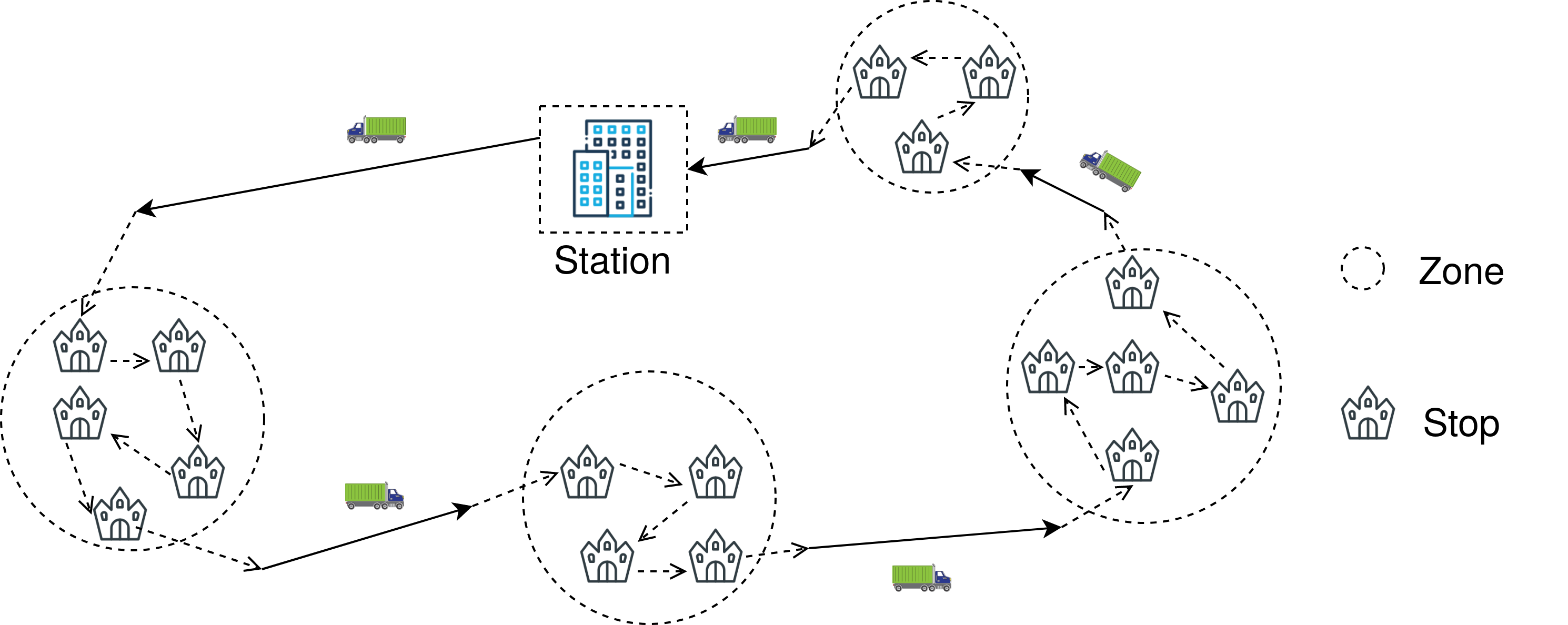
Figure 1: The schematic diagram of the two stage TSP approach with zone and stop ordering

We consider the following setting: there is a set of delivery locations (or stops) denoted by $\mathcal{S}$. At our disposal there is a daily historical set of solutions $\mathcal{H}=\{S_{t},q^{t},x^{t}\}_{t=1}^{T}$, where each $S_{t}\subseteq\mathcal{S}$ is the set of stops at day $t$, and $x^{t}$ indicates the route plan followed on that specific day. Route plans $x^{t}$ (or solutions) are feasible solutions of the travelling salesman problem (TSP) [Miller et al., 1960]. Vector $q^{t}$ states other relevant features of the data of day $t.$ In particular, we consider an optional special attribute namely the drivers’ subjective route quality score which takes values in $\{\mathtt{high,\,medium,\,low}\}$.

The majority of the stops appear only a few times in an $S_{t}$, making it non-viable to directly learn relations between the stops in $\mathcal{S}$. However, stops are partitioned into zones $\mathcal{Z}=\{Z_{1},Z_{2},\ldots,Z_{m}\}$ of the whole territory. This zonification is represented as a partition of $\mathcal{S}$. In other words, $\bigcup_{k=1}^{m}Z_{k}=\mathcal{S}$ and $Z_{k}\cap Z_{k^{\prime}}=\emptyset$ for $k\neq k^{\prime}$. This situation is depicted in Figure 1. As zones cluster stops together, the historical data will have frequently re-occuring zone-to-zone transitions creating the possibility to learn zone transition preferences.The goal is to build a model such that given a new set of stops $S$ the model returns a routing plan $x$ that largely follows the zone-level preferences of the planners and drivers as well as taking the total route distance into account.

We propose a two-stage TSP approach to solve this problem: one TSP over the zones, and a second one over the stops that takes into consideration the sequences of zones. These two TSPs involve three learning processes: two to learn preferences over zones and one to learn good zone penalties when solving the stop-level TSP.

A diagram of the methodology is depicted in Figure 2. We first assume that preferences can be captured as costs of going from one zone/stop to another zone/stop. This assumption is standard as it is used in Canoy & Guns [2019], Mandi et al. [2021], Chen et al. [2021]. One of the advantages of this assumption is the possibility to use exact and/or approximate algorithms available for the TSP. We then estimate zone transition probabilities from historical data, as well as learning the best weighted combination of the zone distance matrix and the zone preference matrix, using structured output prediction [BakIr et al., 2007]. With this zone cost matrix, a sequencing of zones is obtained by solving a zone-level TSP. In the next stage, we use the computed zone sequence to define a zone penalty matrix, penalizing stop-level transitions that do not respect the computed zone ordering. The weights of these penalties are again learned using structured output prediction. Together, this forms the stop cost matrix, where a TSP solver is used to computed the routing over all stops (potentially with time-windows and other operational constraints).

Thus, in our approach there are two TSPs to solve: the first one to determine a sequence of zones, and the second one to route over the stops considering the zone sequencing.

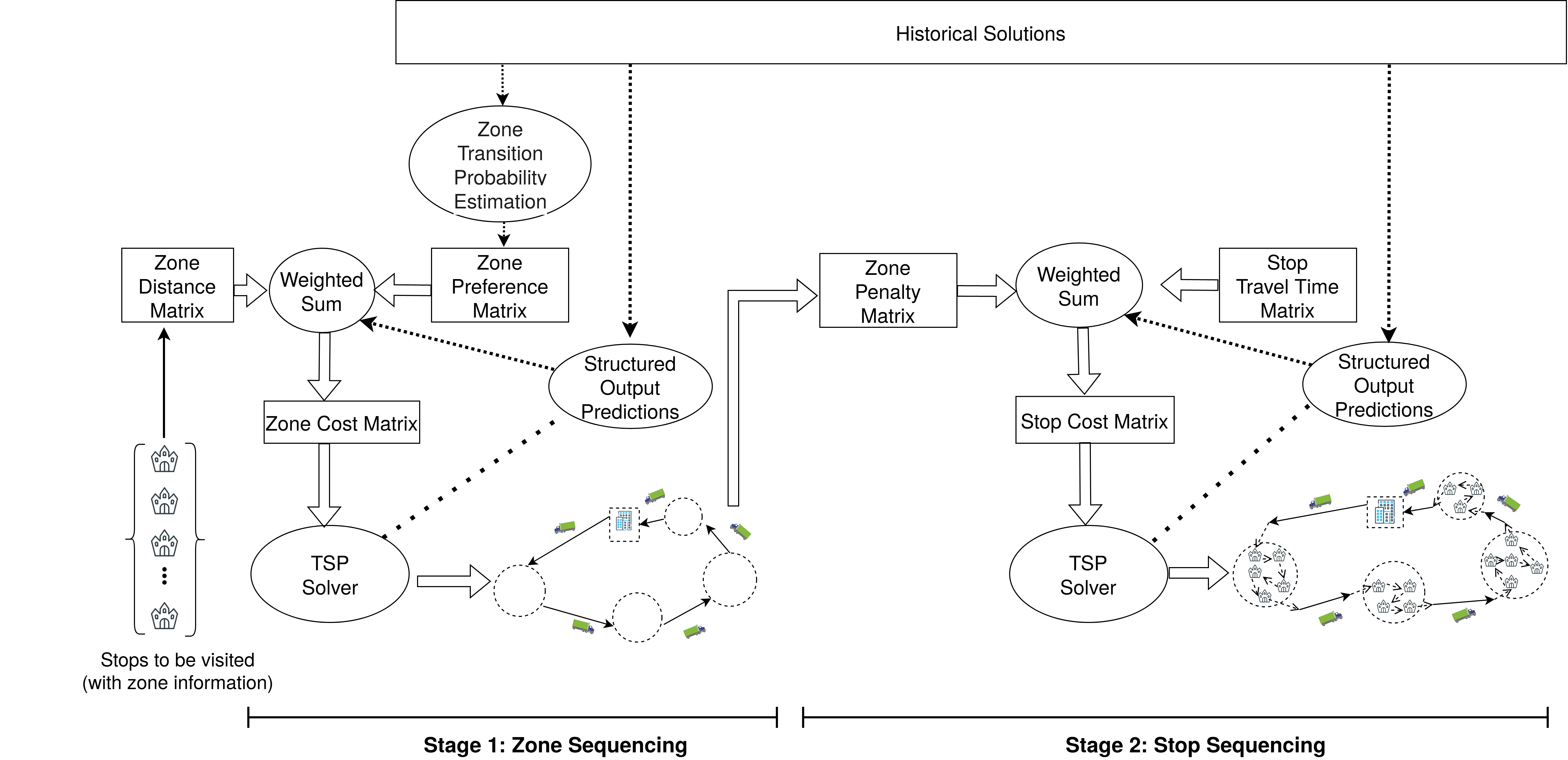
Figure 2: Diagram of the proposed methodology

The contributions of our work are the following:

• We propose a two-stage TSP approach where we learn probabilistic preferences between zones, and use these preferences in defining the penalties in the TSP.

• We estimate transition probabilities with a Markovian counting method, and augment it with structured output prediction [BakIr et al., 2007] to learn appropriate penalties that trade-off distances and learned preferences at the zone level.

• We compute a zone-ordering but do not enforce it as hard constraints. Instead, we penalize zone-order violations and learn the penalties over historic training data.

• We experimentally show the suitability of learning only at the zone level, as well as the benefits of structured output prediction to learn both at the zone level and stop level, on the real data set.

2 Literature Review

The last mile delivery [Zeng et al., 2019] problem has been well studied in the literature. Because of its extensive use in e-commerce, it has received increasing attention in recent years. Last mile delivery may be viewed as a travelling salesman problem (TSP) [Miller et al., 1960] or a vehicle routing problem (VRP) [Dantzig & Ramser, 1959], for which there are many existing available solvers.

However, Li & Phillips [2018] state that in most cases, the last mile delivery does not go according to the planned schedule. In the context of routing between point to point, Ceikute & Jensen [2013] highlight that drivers tend to follow frequently used routes, which are not necessarily shorter in terms of distance or travel time. This is primarily because, in deciding their routes, drivers consider factors which are not in the objective function, e.g., traffic congestion and availability of parking and fuel stations. Drivers have tacit knowledge of this information. Toledo et al. [2013] also point out that drivers tend to rely on tacit knowledge to plan their routes. Explicit formalization of their knowledge poses an insurmountable task.

Several works have studied the problem of learning the routing preferences of the drivers from past routing trajectories. Delling et al. [2015] present a customizable route planning framework that infers the preferences of the drivers from GPS traces by learning individualized cost functions. Letchner et al. [2006] compute the ratios of the individual drivers’ travel time and the theoretical optimal travel time to learn the implicit preferences and biases. Both of the above-mentioned studies focus on point to point commute for individual drivers.

Canoy & Guns [2019] approach the problem in a vehicle routing setting from a different perspective—they introduce a weighted Markov model to learn the preferences from historical routes. This technique avoids the need to explicitly specify the preference constraints and implicit sub-objectives. Their Markovian model computes the transition probabilities between the stops. The model is then used to solve a maximum likelihood routing problem to come up with a routing scheme. We extend this framework to develop a two-stage TSP, where in the first stage we adapt the technique to compute the transition probabilities between zones to find the zone order.

3 Background: the Traveling Salesman Problem (TSP)

Given a set $S$ of stops, with (assymetric) costs $c_{ij}$ associated to each $(i,j)$-pair of stops, the TSP consists of determining a minimum cost circuit passing through each vertex once and only once [Miller et al., 1960, Laporte, 1992]. An integer programming formulation to solve the TSP is:

$$\mathrm{(TSP)}\quad\, \min\sum_{i\neq j}c_{ij}x_{ij}$$ (1)

subject to $$\sum_{j\in S}x_{ij}=1 i\in S,\ i\neq j$$ (2)

$$\sum_{i\in S}x_{ij}=1 j\in S,\ j\neq i$$ (3)

$$\sum_{i,j\in V}x_{ij}\leq|V|-1 V\subset\{1,\ldots,n\},\ 2\leq|V|\leq|V|-2$$ (4)

$$x_{ij}\in\{0,1\} i,j\in S,\ i\neq j$$ (5)

where the variable vector $x$ is defined as above. The objective function minimizes the sum of the cost over the arcs in the route. The first two constraints ensure that each stop is visited onle once. The third constraint ensures that there are no subtours in the solution.

Our approach does not rely on an integer programming formulation, but works with any TSP solver. By abuse of notation, we will refer to TSP$([c_{ij}])$ as an anytime oracle that returns an optimal solution of (TSP) when the cost vector $c$ is optimized, or the best one found in case a timelimit is reached.

Several exact methods and heuristics are being developed to solve this problem since the 60s, making it one of the most studied problems in operations and transportation research Applegate et al. [2011].

4 Methodology

In this section we describe in detail our methodology to learn and implement the two-stage TSP. Figure 2 shows the overview, where the first learning stage, zone ordering, consists in catching preferences over transitions between zones. These preferences are modelled as a linear combination of two terms: the first one related to the distance between zones, and a second one which is a function of the frequency with which each transition appears in the data training. We then apply an structured output prediction approach to learn the weights in the linear combination. The second stage, stop ordering, consists in learning how to route over stops taking into account a predefined zone ordering. This task is performed by setting penalties each time that a solution does not respect the zone ordering. The values of this penalties are also learnt by structured output prediction.

4.1 Stage 1. Zone ordering.

The first phase of our proposed two-stage approach is the zone ordering phase. Given the set of stops (delivery locations), with each stop assigned to a zone, our goal at this stage is to generate a good zone order. Note that zones need not be supplied by the user per se, one could use a clustering method, or geographical regions too. The main point is to make the number of regions of interest (stops/zones) less sparse, so that learning a function that can be applied in new unseen situations becomes more meaningful.

4.1.1 Zone order by distance

A direct approach to get a sequence of zones is to use the distance between them, and minimizing the distance of visiting all of them. Given a set of stops $S$ and the corresponding set of zones $Z_{1},\ldots,Z_{m}$ that contain the stops, we solve a TSP to visit each zone. In this case, we use as a cost $c_{ij}$ in Equation (1) the euclidean distance between the centroid of zone $Z_{i}$ and $Z_{j}$, noted by $d_{ij}$. Formally, if the stops inside the zone $Z_{i}=\{s_{1},\ldots,s_{|Z_{i}|}\}$ are geolocated with coordinates $q^{long}(s),q^{lat}(s)$, then the centroid is given by:

$$q^{long}(Z_{i})=\frac{1}{|Z_{i}|}\sum_{s\in Z_{i}}q^{long}(s),\quad q^{lat}(Z_{i})=\frac{1}{|Z_{i}|}\sum_{s\in Z_{i}}q^{lat}(s).$$ (6)

As the coordinates of the stops within a zone are relatively close to one another, we treat the earth as being locally flat and determine the centroid by taking the average of the latitudes and the longitudes of all the stops. Then, the distances $D=[d_{ij}]$ are given by

$$d_{ij}=\sqrt{\left(q^{long}(Z_{i})-q^{long}(Z_{j})\right)^{2}+\left(q^{lat}(Z_{i})-q^{lat}(Z_{j})\right)^{2}}$$ (7)

Note that this zone sequencing by distance approach does not make use of the historical data. There is no learning involved, hence the method is able to provide a solution for any given instance without any model training. While this traditional approach indeed gives the distance-wise optimal zone sequence, there is no guarantee that the resulting order is close to that of the expert-made solution.

4.1.2 Zone order using transition probabilities

Learning zone order from historical data

We adapt the approach introduced in Canoy & Guns [2019] of learning transition probabilities between zones from the historical data. This approach models preferences as a Markov chain, where the preferences are learnt as the probability of going from one zone/stop to another. The idea is that by determining the zone transition probabilities, we are implicitly learning the latent preferences of the expert.

Let us denote $\mathbf{P}$ the transition probability matrix, where each component $P_{ij}$ represents the probability of going from zone $Z_{i}$ to $Z_{j}$. While the probabilistic model is relatively simple, it allows us to construct a zone transition probability matrix. Solving (TSP) using this transition matrix will give us the maximum likelihood zone sequence. This maximum likelihood problem can be cast as:

$$\max_{x}\prod_{(i,j)}P_{ij}x_{ij}:\quad x\mbox{ satisfies \eqref{eq:flow1} - \eqref{eq:natx}},$$ (8)

which is equivalent to solve a TSP with $c_{ij}=-log(P_{ij})$ in (1), as $\max_{x}\prod_{(i,j)}P_{ij}x_{ij}=\min_{x}\sum_{(i,j)}-log(P_{ij})x_{ij}$. So the model is compatible with any TSP solver. Now we focus on how the transition probability matrix $P$ is obtained.

Input : Set $\mathcal{H}=\{S_{t},q^{t},x^{t}\}_{t=1}^{T}$ of actual traversed routes from historical data; Optionally, per-instance weights $v^{t},$ that influence the importance of the instance.

Output : Zone transition probability matrix $\mathbf{P}$

1 for each $x^{t},$ $t=1,\ldots,T$ do

2       Construct an adjacency matrix $\mathbf{A}^{t}=[a^{t}_{ij}],$ where $a^{t}_{ij}=1$ if the transition $(Z_{i}\rightarrow Z_{j})$ is in $x^{t},$ and $0$ otherwise.

3 end for

4Build the zone transition frequency matrix $\overline{\mathbf{P}}=[\overline{p}_{ij}]$ by (weighted) counting over the the adjacency matrices constructed in the previous step

$$\overline{\mathbf{P}}=\sum_{k=1}^{p}v^{t}\mathbf{A}^{t}.$$ (9)

5 Normalize rows of $\overline{\mathbf{P}}$ by dividing each element by the row sum to obtain the zone transition probability matrix:

$$p_{ij} =\frac{\overline{p}_{ij}}{\sum_{k}\overline{p}_{ik}}.$$

return Zone transition probability matrix $\mathbf{P}=[p_{ij}],$ where $p_{ij}=\text{probability of }(Z_{i}\rightarrow Z_{j})$

Algorithm 1 Building the zone transition probability matrix

Transition probability matrix construction algorithm

Algorithm 1 outlines the process of constructing the zone transition probability matrix from historical data. Let $\mathcal{H}=\{S_{t},q^{t},x^{t}\}_{t=1}^{T}$ denote the set of historical routes and $\mathcal{Z}=\{Z_{1},\ldots,Z_{m}\}$ the zonification.

We build a transition probability matrix $\mathbf{P}\in[0,1]^{m\times m}$ by computing a weighted frequency of appearance of each transition between zones. The algorithm works as follow: For each route $x^{t}$, an adjacency matrix $\mathbf{A}^{t}$ is built where $a^{t}_{ij}$ equals to 1 if the transition $Z_{i}\rightarrow Z_{j}$ occurs, and 0 otherwise. Then, a matrix $\overline{\mathbf{P}}$ is built by summing over all the adjacency matrices weighted by instance-specific parameters $v^{t}$. Finally, the transition probability matrix $\mathbf{P}$ is obtained after normalization.

When a route quality score, e.g., $\{\mathtt{high,\,medium,\,low}\},$ is associated to each route, we can control how much the zone sequence contained in each route influences the resulting zone transition probability matrix (step 4 of Algorithm 1). This can be achieved by allocating a larger weight to $\mathtt{high}$ quality routes (and a smaller weight to $\mathtt{low}$ quality routes). For example, we can assign numerical weights $\{v_{\mathtt{high}},\,v_{\mathtt{medium}},\,v_{\mathtt{low}}\}$ corresponding to each of the score labels $\{\mathtt{high,\,medium,\,low}\},$ where $v_{\mathtt{high}}\geq v_{\mathtt{medium}}\geq v_{\mathtt{low}}.$ Alternatively, we can train selectively with only the $\mathtt{high}$ quality routes by setting $v_{\mathtt{high}}=1$ and $v_{\mathtt{medium}}=v_{\mathtt{low}}=0,$ etc.

4.1.3 Zone order by mixing distances and transition probabilities

We take inspiration from Canoy & Guns [2019] where experimental results show that a cost matrix that mixes (1) distances and (2) transition probabilities, can lead to better solutions being found. From an application point of view, this is motivated by the observation that planners have personal and experience-based preferences, but also always take the total distance into account. From a probabilistic inference perspective, it could be that the estimated probability matrix is uncertain (or indifferent) with respect to certain stops/zones, for example, new stops that have rarely (or even not) been visited before. This too suggests it can be beneficial to combine distances with the estimated probabilities.

The formulation of the cost matrix $[c_{ij}]$ for the TSP is then:

$$c_{ij}=-w_{d}log(d^{\prime}_{ij})-w_{p}log(p_{ij})$$ (10)

where $\mathbf{P}$ is the estimated preference matrix and $\mathbf{D}^{\prime}=[d^{\prime}_{ij}]$ is a distance-based probability matrix.

In our distance-based probability, we want stops that are closer together (so with small $d_{ij}$) to have higher probability than stops that are far apart. We hence first invert the distance and then normalize the rows so they sum up to $1$:

$$d^{\prime}_{ij}=\frac{1/d_{ij}}{\sum_{k}1/d_{ik}}.$$ (11)

Both values are in the interval $[0,1]$, but it is nonetheless impossible to know upfront how to best mix them, that is, what values of $(w_{d},w_{p})$ will result in a cost matrix $[c_{ij}]$ leading to the best zone routing.

We propose a principled way to learn the $(w_{d},w_{p})$ values from historic data. The key challenge here is that we do not know what the true cost matrix $[c^{*}_{ij}]$ is. If this would have been the case, we could have treated the weight learning as a standard machine learning regression problem.

Instead, we only know for each historic routing, what the followed zone tour $x^{*}$ was; and that a given $(w_{d},w_{p})$ tuple leads to a cost function $[c_{ij}]$ for which we can compute the optimal zone tour using a TSP solver. In other words, the actual values of the predicted $[c_{ij}]$ do not matter, only the resulting tour x as the optimal solution of TSP$([c_{ij}])$. We observe that this can be seen as a structured output prediction problem.

Structured output prediction is used in a setting where given an input, we want to predict an output that satisfies a predefined structure. For instance, in case of part of speech (PoS) tagging, the input is a sentence and the output is the sequence of PoS tags, which must have the combinatorial and compositional structure of the English language. In this case, treating the PoS tag of each word independently ould be inefficient as such an approach would fail to capture the expressivity of the language. The structured output prediction approach, on the other hand, predicts PoS tags of multiple words simultaneously and utilizes the dependencies between them to maintain the linguistic structure in the output BakIr et al. [2007]. Structured output prediction has been successfully used in complex applications such as semantic parsing in natural language processing [Clarke et al., 2010], semantic role labeling [Yadollahpour et al., 2013] and computational biology [Chen et al., 2020].

In our case, the predefined structure is that the prediction has to be a circuit that visits every stop exactly once: a feasible TSP solution. In general, in structured output prediction, the problem of searching for a score-maximizing output structure (called the inference task) is the following:

$$\hat{x}=\operatorname*{arg\,max}_{x\in\mathcal{X}(u)}f(x;\mathbf{w},u)$$ (12)

where $u$ is the input (in our case: the set of zones to route over, as well as the pairwise distance and any other relevant information), $\mathcal{X}(u)$ is the (implicit) space of all possible outputs that satisfy the structural constraints (e.g. the feasible solutions of the TSP defined implicitly by (2) - (5)) and $\mathbf{w}$ are the model parameters that we wish to learn. Without loss of generality we will assume that $f$ needs to be maximized to stay close to the traditional structured output prediction literature, (In contrast to the literature, we write $(u,x)$ to denote input/output structure instead of $(x,y)$ as $x$ is more natural for the TSP (output) variables in this paper), even though the TSP is formulated to minimize its cost matrix (or equivalently maximize its -cost matrix).

Many approaches to structured output prediction use approximate inference techniques, for example using the Viterbi algorithm to decode a sequence [BakIr et al., 2007]. However, TSPs have a peculiar structure and very efficient specialised solvers that are often anytime, meaning they can be interrupted with a timeout and will return the best solution found so far. We hence do not mind calling a TSP solver repeatedly during learning.

We will use the seminal structured perceptron algorithm of Collins (see Collins [2002]). It is a variant of the perceptron algorithm, which in turn forms the basis of neural network learning. While it is restricted to learning a linear function over its input, this is sufficient for our needs. It furthermore has nice convergence properties in case of separable data, similar to the perceptron algorithm [Collins, 2002].

We assume given a dataset $\mathcal{H}=\{(u,x)\}$ of $T$ training examples with $u$ corresponding to an input structure, and $x$ the intended output structure, where $x\in\mathcal{X}(u)$.

The structured perceptron algorithm requires to define a problem specific representation function $\Phi$ that maps every valid $(u,x)$ to a feature vector $\Phi(u,x)$. The length of the feature vector determines the length of the weight vector $\mathbf{w}$, in such a way that the linear function $\mathbf{w}^{\intercal}\Phi(u,x)$, where $\mathbf{w}^{\intercal}\Phi(u,x)$ is the inner product $\sum_{s}w_{s}\Phi_{s}(u,x)$ for a feature vector of length $s$, represents the quality of the input-output pair $(u,x)$. In other words, the structured perceptron algorithm assumes that $f(x;\mathbf{w},u)=\mathbf{w}^{\intercal}\Phi(u,x)$ such that the inference task becomes:

$$\hat{x}=\operatorname*{arg\,max}_{x\in\mathcal{X}(u)}\mathbf{w}^{\intercal}\Phi(u,x)$$ (13)

The learning task is to set the weight values $\mathbf{w}$ using the training examples as evidence.

Before looking at the structured perceptron algorithm, we will translate its required input to our TSP setting:

• $x$ is a TSP solution, represented by an $n\times n$ adjacency matrix $x=[x_{ij}]$;

• $u$ is the input structure, namely the tuple $(n,\mathbf{D}^{\prime},\mathbf{P})$ with $n$ is the number of stops in the instance, $\mathbf{D}^{\prime}$ the normalized distance matrix between the $n$ stops, and $\mathbf{P}$ the estimated probability matrix between the $n$ stops;

• $\mathbf{w}$ is the length-2 weight vector $\mathbf{w}=[w_{d},w_{p}]$ that trades-off the importance of the distance and the probability in determining the TSP quality;

• $\Phi(u,x)$ hence needs to compute a length-2 feature vector such that $\max\mathbf{w}^{\intercal}\Phi(u,x)$ corresponds to $\min\sum_{ij}-w_{d}log(d^{\prime}_{ij})-w_{p}log(p_{ij})$ from Equation (10). We define

  $$\Phi\left(u,x\right) =\Phi\left((n,[d^{\prime}_{ij}],[p_{ij}]),[x_{ij}]\right)$$ (14)

  $$=\left[\sum_{ij}log(d^{\prime}_{ij})x_{ij},\sum_{ij}log(p_{ij})x_{ij}\right]$$ (15)

We can now show that

$$\hat{x} =\operatorname*{arg\,max}_{x\in\mathcal{X}(u)}\mathbf{w}^{\intercal}\Phi(u,x)$$ (16)

$$=\operatorname*{arg\,max}_{x\in\mathcal{X}(u)}w_{d}\sum_{ij}log(d^{\prime}_{ij})x_{ij}+w_{p}\sum_{ij}log(p_{ij})x_{ij}$$ (17)

$$=\operatorname*{arg\,min}_{x\in\mathcal{X}(u)}\sum_{ij}(-w_{d}log(d^{\prime}_{ij})-w_{p}log(p_{ij}))x_{ij}$$ (18)

$$=\mbox{TSP}([c_{ij}])\quad\mbox{with}\quad c_{ij}=-w_{d}log(d^{\prime}_{ij})-w_{p}log(p_{ij})$$ (19)

The structured perceptron algorithm learns $\mathbf{w}$ given a dataset $\mathcal{H}=\{(u,x)\}$ and a representation function $\Phi(u,x)$. The pseudo-code is shown in Algorithm 2.

1 initialize $\mathbf{w}$

2 for $e=1,\ldots,E$ do

3       for all $(u,x)\in\mathcal{H}$ do

4             $\hat{x}\leftarrow\operatorname*{arg\,max}_{\hat{x}\in\mathcal{X}(u)}\mathbf{w}^{\intercal}\Phi(u,\hat{x})$

5             if $\hat{x}\neq x$ then

6                   $\mathbf{w}\leftarrow\mathbf{w}\,+\,\delta\left(\Phi(u,x)-\Phi(u,\hat{x})\right)$

7             end if

8            

9       end for

10      

11 end for

return $\mathbf{w}$

Algorithm 2 The Structured Prediction Algorithm

The weight vector is initialized on line 1, e.g. to constant values such as $0$ or $1$. In every epoch $e$, the algorithm then iterates over the training examples in $\mathcal{H}$ (line 3). It first computes the predicted TSP $\hat{x}$ of the given instance for weight vector $\mathbf{w}$. If the predicted output does not match the intended TSP $x$, then a small perceptron update to the weights $\mathbf{w}$ is performed, using the difference between the representation function $\Phi(u,x)$ of $u$ with the true structured output $x$ and $\Phi(u,\hat{x})$ of $u$ with the predicted output $\hat{x}$. The $\delta$ is the learning rate: a small value that controls how large or small the weight updates are in each iteration. This procedure is repeated for $E$ epochs.

In the experiments, we will evaluate in how far the use of structured output prediction on the weights $\mathbf{w}$ can improve the zone ordering sequence found.

4.2 Stage 2. Stop ordering.

Up to now we discussed how in stage 1 we can estimate the transition probability between zones from historical data, and how we can learn the trade-off between distance and learned probability to obtain good zone-level TSP tours. The goal in this second stage is to find a TSP tour over all the stops, taking the predicted zone ordering of the previous stage into account.

4.2.1 Stop order by minimizing travel time

A direct approach in finding a candidate stop order for a given instance, i.e., a set of stops, is by solving (TSP) with the stops as the vertices, and the given distance or travel time matrix as the cost matrix. Again, here, only the pairwise travel times are taken into account; there is no clustering, as the zones associated to the stops are not considered, nor is there any learning from historical data. Hence, while this method results in a stop sequence that is optimal in terms of the total travel time, there is no assurance that its results are close to the ones made by the expert.

4.2.2 Stop order with zone penalties

At this stage, we propose to add to the travel times between stops some zone penalty, which we can decompose into different penalties for different degrees of order violation compared to the zone ordering of the previous stage.

Let us suppose the following:

• ZO, the zone order obtained in stage 1. This function returns ZO$(Z)=k$ if the zone $Z$ is visited in the k-th order.

• $S=\{s_{0},s_{1},s_{2},\ldots,s_{n}\},$ the set of stops that need to be routed, with $s_{0}$ denoting the depot

• $\mathbf{D}=[d_{ij}],$ a travel time matrix whose $(i,j)$-th element represents the time to travel from stop $s_{i}$ to stop $s_{j}$

To find our desired stop order, we minimize the total travel time while giving some penalty for each transition from one zone to the next. The weight of these penalties will depend on the zone order ZO obtained in stage 1.

We propose to formulate the cost matrix $[c_{ij}]$ for the second stage TSP as a weighted combination of the distance $d_{ij}$ between stop $i$ and $j$ and how the zones of the two stops are related to the computed zone ordering.

The zone ordering induces an order, also on the stops. Let us define the order index function $O:S\rightarrow\{1,\ldots,m\}$, where $O(s_{i})$ (or simply $O_{i}$) is equal to $k$ if $s_{i}\in Z$ and ZO$(Z)=k$. Thus, $O_{i}$ indicates the order where a stop has to be visited. We can now check that two stops $i,j$ belong to the same zone, by checking that $O_{i}==O_{j},$ which is equivalent to checking $Z_{i}==Z_{j}$. Furthermore, we can check whether the zone of stop $j$ is the ‘next’ zone in the zone order, compared to the zone of $i$, in which case: $Z_{j}==Z_{i}+1$ is true. Similarly, we can compute whether $j$ is in the ‘previous’ zone according to $ZO$, or two zones ahead, etc.

Using the zone order index $O_{i}$ and the logical expressions just introduced, we can now define a penalized cost matrix for the stop-level TSP as follows:

$$c_{ij} =\mathbf{w}_{0}d_{ij}+\mathbf{w}_{1}\llbracket O_{i}==O_{j}\rrbracket$$

$$+\mathbf{w}_{2}\llbracket O_{j}==O_{i}+1\rrbracket+\mathbf{w}_{3}\llbracket O_{j}==O_{i}+2\rrbracket$$

$$+\mathbf{w}_{4}\llbracket O_{j}==O_{i}-1\rrbracket+\mathbf{w}_{5}\llbracket O_{j}==O_{i}-2\rrbracket$$

$$+\mathbf{w}_{6}\llbracket O_{j}\geq O_{i}+3\ \textbf{ or }\ O_{j}\leq O_{i}-3\rrbracket$$ (20)

where $\llbracket\cdot\rrbracket$ is the Iverson bracket, it returns $1$ if the logical statement in the bracket is true, and $0$ otherwise. Note how for every pair of stops $i$ and $j$, only one of the Iverson brackets will return the value $1$, the others will be $0$. Hence, this function allows to put different penalties on different kinds of zone order violations.

One approach to set penalty weights $w$ is to choose them manually. For example, if we want to produce routing plans prone to follow the sequencing while minimizing total travel time, we could set $\mathbf{w}_{0}=1,\mathbf{w}_{1}=0,\mathbf{w}_{2}=0$ and all other weights to $+\infty$ (or a very large value).

Alternatively, the zone order penalties could decrease step-wise for larger gaps between the zones of subsequent stops. This could allow “jumps” between adjacent zones, as observed in a number of the actual expert solutions (see also data analysis in the experiment section). However, determining the right penalty values is tedious, prone to error and bias, and is even more difficult to keep up-to-date over time.

4.2.3 Learning penalty parameters via SOP

Given the weighted penalty function, just like in the zone-order TSP case, we can learn these weight penalties automatically on a training set. For this, we can again use Structured Output Prediction; more specifically, the structured perceptron algorithm described in the previous section.

We now provide a mapping to the required input of the perceptron algorithm:

• $x$ is again a TSP solution, represented by an $n\times n$ adjancency matrix $x=[x_{ij}]$ (in this case, over the stops instead of over the zones);

• $u$ is the input structure, for which in this case we propose the tuple $u=(n,D,O)$ where $n$ is the number of stops in the instance, $D$ the travel time matrix between the $n$ stops, and $O$ the zone order index of the $n$ stops;

• $\mathbf{w}$ is the length-7 weight vector $\mathbf{w}=[w_{0},\ldots,w_{6}]$ that balances the importance of the distance and the different penalties;

• $\Phi(u,x)$ is the length-7 feature vector which computes the total distance as well as the total number of violations of every type; we define

  $$\Phi\left(u,x\right) =\Phi\left((n,[d_{ij}],[O_{i}]),x\right)$$ (21)

  $$=\left[\sum_{ij}T_{ij}x_{ij},\sum_{ij}\llbracket O_{i}==O_{j}\rrbracket,\sum_{ij}\llbracket O_{j}==O_{i}+1\rrbracket,\ldots,\sum_{ij}\llbracket O_{j}\geq O_{i}+3\ \textbf{ or }\ O_{j}\leq O_{i}-3\rrbracket\right]$$

From this, as in the previous section, we can similarly derive

$$\hat{x} =\operatorname*{arg\,max}_{x\in\mathcal{X}(u)}\mathbf{w}^{\intercal}\Phi(u,x)$$

$$=\operatorname*{arg\,max}_{x\in\mathcal{X}(u)}\sum_{ij}c_{ij}x_{ij},\quad\mbox{with }c_{ij}~{}\mbox{as defined in Equation~{}\eqref{penalty_obj}}$$

$$=TSP([c_{ij}]).$$

We want to stress that although Equation (20) contains logical expressions, every $O_{i}$ is a constant for a given zone ordering $ZO,$ hence every computed $c_{ij}$ is also a constant. While the equation looks like a multi-objective formulation, and it is a multi-objective formulation, each of the sub-objectives is over the same $x_{ij}$ variables and hence this ‘multi’ objective formulation can be equivalently rewritten as a single linear function over the $x_{ij}$ variables.

5 Numerical Results

We now turn to evaluating the performance and benefits of our proposed approach.

Data description

For an empirical evaluation of the proposed methodology, we conduct our experiments on data provided by Amazon for the Last Mile Routing Challenge . The provided data consists of 6112 historical routes. Each route is a feasible TSP solution which starts and ends at a station, and visits from 31 to 238 stops. As displayed on Fig. 3(a) the distribution of routes between the 17 stations is not uniform. Fig. 3(b) shows how stops are shared between stations. All stops are clustered into 8868 zones. Planning experts assigned a quality score label (high, medium, low) to each route.Vehicle capacities, times of departure and time windows of stops were not considered, although they can be added to the TSP solver without changes to the methodology.

We can extract a zone ordering from each route and empirically observe transitions between (non)adjacent zones. Table 1 denotes the frequency of such transitions. next and prev respectively stands for moving ahead and backward according to the zone ordering. next2 and prev2 denote moving two steps in the related direction. next3+ and prev3+ account for three or more steps, which is a more blatant zone order violation. As displayed on Table 1, those are more common in lower quality route. Medium-quality routes respectively have on average $0.073\%$ and $0.178\%$ of those transitions, against only $0.071\%$ and $0.168\%$ for high-quality routes. The small amount of low-quality routes available does not allow for a fair comparison. Nevertheless, this observation substantiates the underlying hypothesis that more zone order violations in a route lead to worse route quality, and that different penalties for different order violations are sensible.

Scoring

The Amazon challenge scoring function computes the similarity between the actual (zone or stop) sequence and an algorithm-produced sequence. The computation combines Sequence Deviation and Edit Distance with Real Penalty:

$$\mathtt{score}=\frac{SD(A,B)\cdot ERP_{norm}(A,B)}{ERP_{e}(A,B)},$$

where $A$ is the actual sequence and $B$ is the user-submitted sequence. $SD$ denotes the Sequence Deviation of $B$ with respect to $A$, $ERP_{norm}$ denotes the Edit Distance with Real Penalty applied to sequences $A$ and $B$ with normalized distance or travel times, and $ERP_{e}$ denotes the number of edits prescribed by the algorithm on sequence $B$ with respect to $A.$

System description

All experiments were run on a Lenovo ThinkPad X1 Carbon with an Intel Core i7 processor running at 1.8GHz with 16GB RAM. As TSP solver, we used OR-Tools 9.0 with the guided local search as the search strategy. During SOP training and to compute the final zone and stop TSPs that are scored, we set a timeout of 30 seconds to each TSP solver call. The timeout is reached for each TSP computation. Probability estimation and the structured perceptron algorithm were implemented in numpy. We used a fixed learning rate of $\delta=10^{-5},$ determined after small-scale experiments on the training data. We train for $e=1$ epoch unless mentioned otherwise.

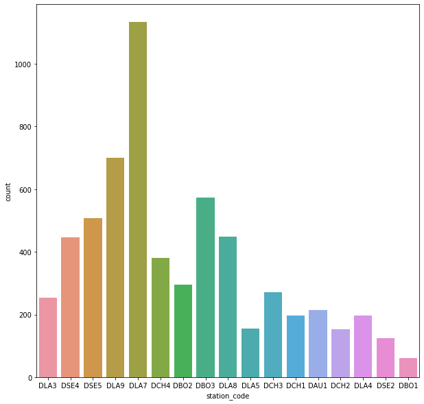
(a) Count of routes per stations

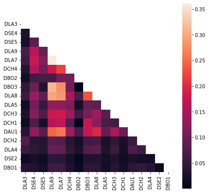
(b) Stops overlap between stations

Table 1: Percentage of stops per route for each kind of zone order transition/violation, as described in Eq. 20

	same	next	next2	next3+	prev	prev2	prev3+
route quality label
high	80.355%	13.552%	0.115%	0.071%	0.209%	0.050%	0.168%
medium	89.295%	13.642%	0.107%	0.073%	0.190%	0.048%	0.178%
low	87.610%	13.668%	0.120%	0.053%	0.174%	0.033%	0.140%

Training and testing set split

Note that we do not have access to the hidden dataset used in the challenge evaluation. We hence conduct our experiments on the historical data which we split into a train and a test set. As each of the 6112 historical instances is tagged with a route quality label, we employ stratified sampling in order to sample each route label subpopulation (high, medium, low) independently.

Table 2: Data partitioned into training and test sets

Route score	Total	Train	Test
high	2718	2174	544
medium	3292	2634	658
low	102	82	20
Total	6112	4890	1222

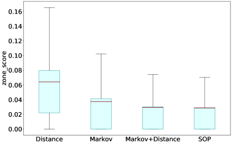
Routes used for training	zone_score
	Distance	Markov	Markov+Distance	SOP
high	0.0642	0.0422	0.0314	0.0317
high + medium	0.0642	0.0371	0.0293	0.0291
high + medium + low	0.0642	0.0374	0.0291	0.0289

Figure 3: Zone scores of zone sequencing approaches on test data

# of epochs	$w_{d}$	$w_{p}$	zone_score
0	1	1	0.0291
1	1.58	2.33	0.0289
2	2.16	3.66	0.0297
3	2.75	4.99	0.0296
4	3.33	6.32	0.0295
5	3.91	7.66	0.0295

Figure 4: Trained weights and corresponding zone scores for different epochs of SOP

Stage 1 experiments: zone-level ordering quality

In the first set of experiments, we test and compare the performance of the different Stage 1 zone sequencing approaches that we presented in the previous section, namely, the distance-based (Distance), transition probabilities/preference-based (Markov), and the mixed distance and transition probabilities (SOP) approaches, where the component weights in the mixed approach are determined by structured prediction.

A graphical visualization of the distribution of the zone scores, as well as a summary of the average zone scores, for the four approaches are shown in Figure 3. Visually, we can already notice a significant improvement when using the Markov model instead of the absolute distance-based approach. Furthermore, when distance and preference components are mixed with equal weight, we get further improved zone scores. The use of Structured Output Prediction (SOP) to find better weights marginally improves the result further. A histogram showing the frequency distribution of the zone scores of the four approaches is shown in Figure 6.

In the table at the bottom of the figure we show the average zone score when using only the high quality labeled routes, or also the medium and low. Although they differ in quality, we can see that using all data results in better overall zone orders. We believe this is due simply to the amount of data available, as can be seen from Table 2.

We take a closer look at the performance of the SOP approach in Figure 4. For this experiment, we ran the structured perceptron algorithm for multiple epochs. In the figure, we can see that starting from uniform weights, the zone score on the test data slightly increases before it worsens again a bit. Looking at the (interpretable) weights, we see that learning especially increases the weight of the prefence matrix compared to the weight of the distance matrix. Runtimes are not shown, but we observed that every instance reaches the timeout of 30 seconds during SOP training.

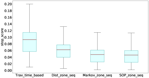
Penalty weights								Zone sequencing approach
$w_{0}$	$w_{1}$	$w_{2}$	$w_{3}$	$w_{4}$	$w_{5}$	$w_{6}$	Trav_time-based	Dist	Markov	SOP
2	1	1.5	2	1.5	2	2	0.0929	0.0617	0.0510	0.0501
2	1	2	4	2	4	6	0.0929	0.0618	0.0507	0.0498
2	0.35	2.13	4.09	2.32	4.02	6.10	0.0929	0.0625	0.0479	0.0465

Figure 5: Stop scores of stop sequencing approaches on test data

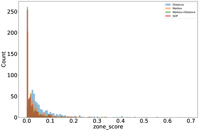
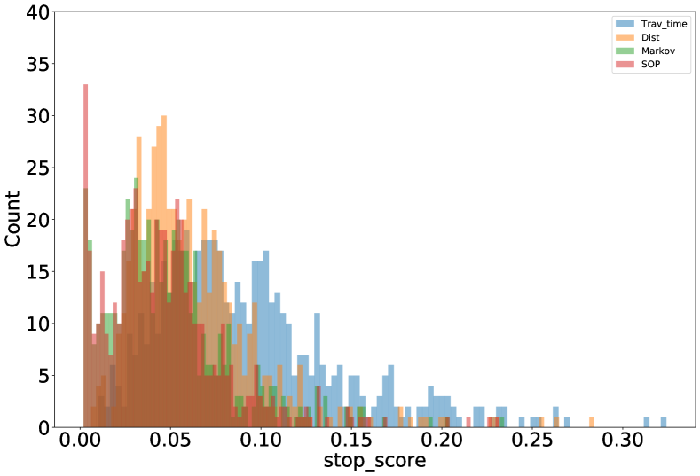
Figure 6: Histograms showing distribution of scores of the stop and zone sequencing approaches

Stage 2: stop-level experiments

The different stage 2 stop ordering approaches are evaluated and compared in this next set of experiments. The first (Trav_time_based) is the conventional approach of solving (TSP) with the given travel time matrix as the cost matrix. The other three are zone penalty approaches, where the zone penalty is determined by the zone order generated in Stage 1.

Numerical results are summarized in Figure 5. The figure summarizes the results, showing that a non-zone based approach using distances performs worst. Even when only using distances, but in a two-stage approach, e.g., zone penalties from a distance-based zone ordering, already leads to improved results. This is in line with our data analysis that a zone ordering is typically followed. Our next two approaches, Markov_zone_seq and SOP_zone_seq differ only in how the zone ordering was computed. As their zone orderings performed rather similar, we also see here that their stop-level scores are also rather similar.

We now look at the effect of different zone penalty weights, at the bottom of Fig 5. We tried two hand-crafted penalty values: one in which the penalty for ‘larger’ zone violations gradually increases (1, 1.5, 2) and one in which it more rapidly increases (1,2,4,6). Finally, the bottom line, which was initialized with the better-performing second row values, shows the output after 1 epoch of SOP learning on these weights. We can see that the best approach is the combination of Markov estimation with SOP both at the zone-level and at the stop-level. Looking at the bottom entry in particular, we can see that the stop-level SOP especially learned to decrease the same-zone penalty weight, as well as increasing ‘previous’ and ‘next’ penalty scores. The histogram in Figure 6 shows the frequency distribution of the stop scores of the four approaches, where most of the scores of the better preforming methods, SOP and Markov, tend to be closer to zero.

6 Concluding Remarks

This article studies the problem of learning the preferences of drivers and planners over a set of delivery locations in the last mile delivery context. The main difficulty of this problem is that clients do not appear often in the historical data, making it impossible to learn transition preferences at the stop level. Hence, we study a setting where stops are clustered into zones. We propose a two-stage TSP approach to solve this problem.

In the first stage, the preferences of transitions between zones are learned from historical data. This allows us to produce sequences of zones aligned to the preferences of the expert users. We adapt from literature a Markovian approach to learn zone transition probabilities and combine these with pairwise zone distances to generate zone sequences that not only minimize the travel distance but also maximizes user preferences. Furthermore, we apply the structured output prediction approach to learn the optimal parameters to be used in combining the distances and the transition probabilities.

In the second stage, we structure the stop routing problem into a TSP whose objective function combines the travel time and zone transition penalties derived from the zone order obtained in the previous stage. As the objective function now takes the form of a weighted multi-objective function, we again see the opportunity to apply structured prediction to fine-tune some initial penalty values.

Our computational results show that compared to the conventional method of stop routing by TSP using travel times, our two-stage zoning approach significantly performs better. Stage 1 experiments confirm that combining distances and transition probabilities result to better zone sequences. Stage 2 experiments show that our proposed zone penalty framework results to higher quality stop sequences. In both sets of experiments, we confirm that we can obtain improved results by using structured output prediction.

Future work will involve applications to other extended settings, such as vehicle routing. Another relevant future research question is to measure the impact in accuracy and computational times of using different methods to solve the TSP either exactly or by heuristics; as well as incremental methods that do not require to re-solve from scratch in every structured-output prediction loop. Another avenue that can be explored is additional features to be used for learning, both at the zone level and the stop level, as well as the use of other structured output prediction methods including deep learning ones. However, more complex learning architectures may also require more training data.

References

- Applegate et al. [2011] Applegate, D. L., Bixby, R. E., Chvátal, V., & Cook, W. J. (2011). The traveling salesman problem. Princeton university press.
- BakIr et al. [2007] BakIr, G., Hofmann, T., Schölkopf, B., Smola, A. J., Taskar, B., & Vishwanathan, S. (2007). Predicting Structured Data. The MIT Press. URL: https://doi.org/10.7551/mitpress/7443.001.0001. doi:10.7551/mitpress/7443.001.0001.
- Canoy & Guns [2019] Canoy, R., & Guns, T. (2019). Vehicle routing by learning from historical solutions. In International Conference on Principles and Practice of Constraint Programming (pp. 54–70). Springer.
- Ceikute & Jensen [2013] Ceikute, V., & Jensen, C. S. (2013). Routing service quality–local driver behavior versus routing services. In 2013 IEEE 14th International Conference on Mobile Data Management (pp. 97–106). IEEE volume 1.
- Chen et al. [2021] Chen, L., Chen, Y., & Langevin, A. (2021). An inverse optimization approach for a capacitated vehicle routing problem. European Journal of Operational Research, .
- Chen et al. [2020] Chen, X., Li, Y., Umarov, R., Gao, X., & Song, L. (2020). RNA secondary structure prediction by learning unrolled algorithms. In 8th International Conference on Learning Representations, ICLR 2020, Addis Ababa, Ethiopia, April 26-30, 2020.
- Clarke et al. [2010] Clarke, J., Goldwasser, D., Chang, M., & Roth, D. (2010). Driving semantic parsing from the world’s response. In M. Lapata, & A. Sarkar (Eds.), Proceedings of the Fourteenth Conference on Computational Natural Language Learning, CoNLL 2010, Uppsala, Sweden, July 15-16, 2010 (pp. 18–27). ACL.
- Collins [2002] Collins, M. (2002). Discriminative training methods for hidden markov models: Theory and experiments with perceptron algorithms. In Proceedings of the 2002 conference on empirical methods in natural language processing (EMNLP 2002) (pp. 1–8).
- Dantzig & Ramser [1959] Dantzig, G. B., & Ramser, J. H. (1959). The truck dispatching problem. Management science, 6, 80–91.
- Delling et al. [2015] Delling, D., Goldberg, A. V., Goldszmidt, M., Krumm, J., Talwar, K., & Werneck, R. F. (2015). Navigation made personal: Inferring driving preferences from gps traces. In Proceedings of the 23rd SIGSPATIAL international conference on advances in geographic information systems (pp. 1–9).
- Joachims [2002] Joachims, T. (2002). Optimizing search engines using clickthrough data. In Proceedings of the eighth ACM SIGKDD international conference on Knowledge discovery and data mining (pp. 133–142).
- Kool et al. [2019] Kool, W., van Hoof, H., & Welling, M. (2019). Attention, learn to solve routing problems! In International Conference on Learning Representations. URL: https://openreview.net/forum?id=ByxBFsRqYm.
- Laporte [1992] Laporte, G. (1992). The traveling salesman problem: An overview of exact and approximate algorithms. European Journal of Operational Research, 59, 231–247.
- Letchner et al. [2006] Letchner, J., Krumm, J., & Horvitz, E. (2006). Trip router with individualized preferences (trip): Incorporating personalization into route planning. In AAAI (pp. 1795–1800).
- Li & Phillips [2018] Li, Y., & Phillips, W. (2018). Learning from route plan deviation in last-mile delivery. Master’s thesis Massachusetts Institute of Technology, Cambridge.
- Lu et al. [2015] Lu, J., Wu, D., Mao, M., Wang, W., & Zhang, G. (2015). Recommender system application developments: a survey. Decision Support Systems, 74, 12–32.
- Mandi et al. [2021] Mandi, J., Canoy, R., Bucarey, V., & Guns, T. (2021). Data driven vrp: A neural network model to learn hidden preferences for vrp. In 27th International Conference on Principles and Practice of Constraint Programming (CP 2021) (p. 42). Schloss Dagstuhl-Leibniz-Zentrum für Informatik.
- Miller et al. [1960] Miller, C. E., Tucker, A. W., & Zemlin, R. A. (1960). Integer programming formulation of traveling salesman problems. Journal of the ACM (JACM), 7, 326–329.
- Toledo et al. [2013] Toledo, T., Sun, Y., Rosa, K., Ben-Akiva, M., Flanagan, K., Sanchez, R., & Spissu, E. (2013). Decision-making process and factors affecting truck routing. In Freight Transport Modelling. Emerald Group Publishing Limited.
- Vinyals et al. [2015] Vinyals, O., Fortunato, M., & Jaitly, N. (2015). Pointer networks. In C. Cortes, N. Lawrence, D. Lee, M. Sugiyama, & R. Garnett (Eds.), Advances in Neural Information Processing Systems. Curran Associates, Inc. volume 28. URL: https://proceedings.neurips.cc/paper/2015/file/29921001f2f04bd3baee84a12e98098f-Paper.pdf.
- Yadollahpour et al. [2013] Yadollahpour, P., Batra, D., & Shakhnarovich, G. (2013). Discriminative re-ranking of diverse segmentations. In 2013 IEEE Conference on Computer Vision and Pattern Recognition, Portland, OR, USA, June 23-28, 2013 (pp. 1923–1930). IEEE Computer Society.
- Zeng et al. [2019] Zeng, Y., Tong, Y., & Chen, L. (2019). Last-mile delivery made practical: An efficient route planning framework with theoretical guarantees. Proceedings of the VLDB Endowment, 13, 320–333.
Acknowledgments
This research received partial funding from the FWO Flanders project grant FWO-S007318N (Data-driven logistics), the European Research Council (ERC H2020, Grant agreement No. 101002802, CHAT-Opt), and the Institute for the encouragement of Scientific Research & Innovation of Brussels (Innoviris, 2021-RECONCILE).