Quantum anomaly detection of audio samples with a spin processor in diamond

Abstract

In the process of machine learning, anomaly detection plays an essential role for identifying outliers in the datasets. Quantum anomaly detection could work with only resources growing logarithmically with the number and the dimension of training samples, while the resources required by its classical counterpart usually grow explosively on a classical computer. In this work, we experimentally demonstrate a quantum anomaly detection of audio samples with a three-qubit quantum processor consisting of solid-state spins in diamond. By training the quantum machine with a few normal samples, the quantum machine can detect the anomaly samples with a minimum error rate of 15.4%, which is 55.6% lower than distance-based classifying method. These results show the power of quantum anomaly detection dealing with machine learning tasks and the potential to detect abnormal instances of quantum states generated from quantum devices.

I Introduction

Machine learning could reveal the patterns in datasets and use them in subsequent tasks. Many pattern recognition tasks focus on the classification of new samples into two or more classes, after training with a similar number of training samples for each class. However, in some realistic problems the training dataset consists of a highly unbalanced number of samples in different classes, which is not suitable for multi-class classification methods. These problems often appear in the form of anomaly detection (AD), such as fraud detection of credit cards, faults detection in complex industrial systems and medical diagnosis et al. In these problems, the normal cases are well sampled and the anomalies are rare and under-sampled. The task of anomaly detection is to learn the pattern of the normal cases and identify that whether a new sample belongs to them. The problem of anomaly detection is often researched in the framework of one-class classification Chandola et al. (2009); Pimentel et al. (2014). Multiple approaches are proposed, such as density estimation method Breunig et al. (2000), k-nearest neighbor Hautamaki et al. (2004), one-class support vector machine Choi (2009) et al. By modelling the well-sampled normal data (training set), one can give an anomaly score for every new sample (test data) to quantify how far away it is from the pattern of the normal data and then identify anomalies based on these scores.

The running of machine learning algorithms often requires dealing with high-dimensional matrices and corresponding linear algebra problems. Due to the natural essence as a linear system, quantum mechanics can be easily used to interpret datasets stored as matrices and perform matrix processing with the help of quantum speedup Harrow et al. (2009); Pan et al. (2014). Running machine learning algorithms on quantum computers leads to an interdisciplinary field called quantum machine learning Dunjko et al. (2016); Biamonte et al. (2017); Dunjko and Briegel (2018); Schuld and Killoran (2019), where quantum algorithms promise to outperform their classical counterparts. Many quantum machine learning tasks such as principal component analysis (PCA) Lloyd et al. (2014); Li et al. (2021), support vector machines (SVM) Rebentrost et al. (2014); Li et al. (2015), generative adversarial network models Lloyd and Weedbrook (2018); Hu et al. (2019); Huang et al. (2021) have been demonstrated algorithmically or experimentally. Recently, quantum algorithms for anomaly detection have been proposed, showing the potential to detect anomalies with resources growing logarithmically with respect to the number of training samples and the dimension of them Liu and Rebentrost (2018); Liang et al. (2019); Herr et al. (2021); Kottmann et al. (2021). By calculating the inner products of multiple samples in parallel, the quantum algorithms can efficiently provide the anomaly score of a new test sample of interest, defined by the proximity measure between the new sample and the given training dataset. After that, one can label the new sample as normal or anomaly according to the anomaly score of it.

In this work, we report an experimental demonstration of the PCA-based quantum anomaly detection (QAD) with a hybrid spin system in diamond at ambient conditions. We apply the algorithm to an audio recognition problem to detect whether a new audio sample is similar to the pattern of previously given samples. Compared to classifying based on the Euclidean distance, our implementation can learn the distribution of the training samples in the feature space. As a result, the error rate of our scheme reaches a minimum of 15.4%, which is 55.6% lower than classifying by only the Euclidean distance.

II Results and discussion

The anomaly detection task discussed in this work is the identification of outlier data that deviate from the pattern of normal data in the feature space. The training set labeled as normal consists of $\mathrm{M}$ training samples $\vec{z}_{i}$ $\{i=1,2,...,\mathrm{M}\}$ and the new sample to be inspected is denoted by $\vec{z}_{\rm test}$. Here each sample is represented by a vector in $\mathrm{d}$-dimension feature space and all the training samples are pre-centralized, i.e., $\sum_{i=1}^{\mathrm{M}}\vec{z}_{i}=\mathrm{0}$. The task of the anomaly detection algorithm is to find an anomaly score for each new sample that can describe how far away it is from the pattern of normal samples. After this, one can set a threshold $\epsilon$ and then classify a sample as anomaly while the anomaly score of it is greater than $\epsilon$.

A simple way to define the anomaly score is to compute the Euclidean distance between the test sample and the centroid of the training data Hodge and Austin (2004) (Fig. 1(a)),

$$g\left(\vec{z}_{\rm test}\right)=\left|\vec{z}_{\rm test}\right|^{2}.$$ (1)

A large Euclidean distance from the centroid predicts that the new sample is likely to be an anomaly case. The definition of Euclidean distance grants the same weight to the deviations in different dimensions, which makes it only works well when the samples have a nearly isotropic distribution in the feature space. On the other hand, if the training data has a sparse distribution in one direction while they are clustered in another direction, the Euclidean distance cannot recognize this anisotropy property. This leads to the possibility that the normal and anomaly samples may have similar Euclidean distances and thus will be misclassified (Fig. 1(b)).

As a well-known technique of multivariate analysis, principal component analysis can reveal the inner structure of data. The PCA-based anomaly detection algorithm analyzes the distribution of the training data in the feature space and quantifies how well the inspected sample fits it. In this scheme, the anomaly score of $\vec{z}_{\rm test}$ is defined by proximity measure $f\left(\vec{z}_{\rm test}\right)$ Liu and Rebentrost (2018), which compares the Euclidean distance $g\left(\vec{z}_{\rm test}\right)$ and the variance of the training data along the direction of $\vec{z}_{\rm test}$:

$$f\left(\vec{z}_{\rm test}\right)=\left|\vec{z}_{\rm test}\right|^{2}-\frac{1}{\mathrm{M}-1}\sum_{i=1}^{\mathrm{M}}\hat{z}_{\rm test}^{T}\vec{z}_{i}\vec{z}_{i}^{T}\hat{z}_{\rm test},$$ (2)

where $\hat{z}_{\rm test}=\vec{z}_{\rm test}/\left|\vec{z}_{\rm test}\right|$. Compared with judging by $g\left(\vec{z}_{\rm test}\right)$, the distribution of the training data is also considered in the second term of Eq. 2. By introducing the covariance matrix

$$C=\frac{1}{\mathrm{M}-1}\sum_{i=1}^{\mathrm{M}}\vec{z}_{i}\vec{z}_{i}^{T},$$ (3)

one can have a more concise expression for the proximity measure

$$f\left(\vec{z}_{\rm test}\right)=\left|\vec{z}_{\rm test}\right|^{2}-\hat{z}_{\rm test}^{T}C\hat{z}_{\rm test}.$$ (4)

Fig. 1(b) shows that the proximity measure can better reveal the pattern of training data since it can provide a boundary line dividing normal and anomaly data that is closer to the distribution of the training data.

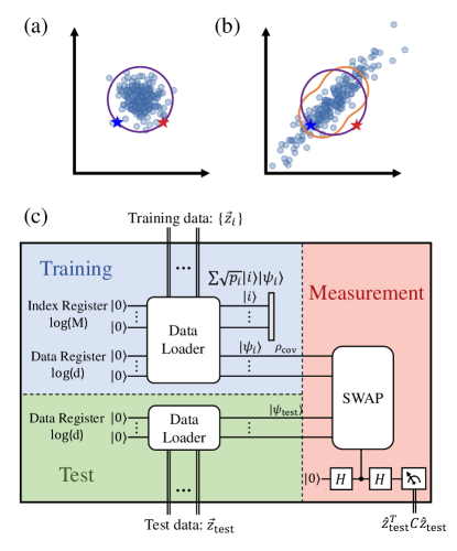
Figure 1: (a) and (b) The training samples labeled as normal in the feature space. The purple line and orange lines represent the boundary lines given by certain values of Euclidean distance and proximity measure, respectively. (c) Schematic diagram of quantum anomaly detection algorithm in this work. The training data and test sample are loaded into the quantum registers and a swap test is used to estimate how close the test sample is from the pattern of the normal samples in the training set.

Now we turn to the quantum version of the anomaly detection algorithm. The QAD algorithm could compute $\hat{z}_{\rm test}^{T}C\hat{z}_{\rm test}$ using resources logarithmic in the dimension of samples ($\mathrm{d}$) and the number of training samples ($\mathrm{M}$) by processing all the vectors in the form of quantum states Liu and Rebentrost (2018). A training-data oracle is employed to load the classical vectors into quantum register, which consists of a data register and an index register (Fig. 1(c)). For each $\mathrm{d}$-dimension vector $\vec{z}_{i}$, the data loader returns a training state $\left|\psi_{i}\right\rangle=1/\left|\vec{z}_{i}\right|\sum_{j=1}^{\mathrm{d}}\left(\vec{z}_{i}\right)_{j}|j\rangle$ and stores it into the data register. Here $|j\rangle$ represents the computational basis, and $\left(\vec{z}_{i}\right)_{j}$ represents the $j\mathrm{th}$ element of the $i\mathrm{th}$ sample. The fast loading of all the $\mathrm{M}$ vectors can be addressed by using quantum random access memory Giovannetti et al. (2008). Starting with the superposition in the index register, $\frac{1}{\sqrt{\mathrm{M}}}\sum_{i=1}^{\mathrm{M}}|i\rangle$, the information of all training samples is stored as a superposition state

$$|\Psi\rangle=\sum_{i=1}^{\mathrm{M}}\sqrt{p_{i}}\ |i\rangle\left|\psi_{i}\right\rangle,$$ (5)

where $p_{i}=\frac{\left|\vec{z}_{i}\right|^{2}}{\sum_{i=1}^{\mathrm{M}}\left|\vec{z}_{i}\right|^{2}}$ represents the normalized module length $|\vec{z}_{i}|^{2}$ of the training data. At this stage, the reduced density matrix of the quantum state in the data register is

$$\rho_{\mathrm{cov}}=\sum_{i=1}^{\mathrm{M}}p_{i}\left|\psi_{i}\right\rangle\left\langle\psi_{i}\right|,$$ (6)

which has the same form as the covariance matrix $C$ in Eq.  3, up to an overall factor $\mathrm{\textbf{tr}}C=\frac{\sum_{i=1}^{\mathrm{M}}\left|\vec{z}_{i}\right|^{2}}{\mathrm{M}-1}$.

Following the same method, the test sample $\vec{z}_{\rm test}$ is loaded into the quantum register in the form of test state $\left|\psi_{\rm test}\right\rangle=\sum_{j=1}^{\mathrm{d}}\left(\hat{z}_{\rm test}\right)_{j}|j\rangle$. Then the proximity measure in Eq.  4 reduces to

$$f\left(\vec{z}_{\rm test}\right) =\left|\vec{z}_{\rm test}\right|^{2}-\mathrm{\textbf{tr}}C\ \sum_{i=1}^{\mathrm{M}}p_{i}|\langle{\psi_{\rm test}}|{\psi_{i}}\rangle|^{2}$$ (7)

$$=\left|\vec{z}_{\rm test}\right|^{2}-\mathrm{\textbf{tr}}C\ \langle\psi_{\rm test}|\rho_{\mathrm{cov}}|\psi_{\rm test}\rangle.$$

Here the second term can be measured by a swap test Buhrman et al. (2001) between $\rho_{\mathrm{cov}}$ and $|\psi_{\rm test}\rangle$, after these two quantum states are prepared in the previous step. By measuring the overlap between these two states, the inner products of the test state and all the training states are calculated simultaneously. In the readout process, the anomaly score can be estimated by measuring the expectation value of the ancillary qubit in the swap test, as shown in Fig. 1(c).

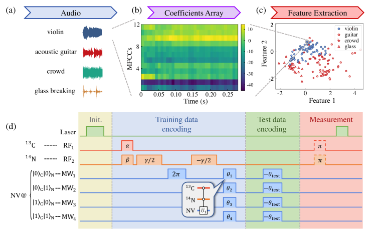
Figure 2: (a-c) The pre-processing of the audio samples. (a) Examples of different types of audio samples and their corresponding waveforms. (b) Cepstral coefficients array extracted from violin-47.wav as an example. Each column represents the MFCCs extracted from one frame of the audio sample. (c) The distribution of all the audio samples in 2-dimension feature space. (d) The experimental circuit of the quantum anomaly detection algorithm. ¹³C and ¹⁴N nuclear spins are utilized as the index register, while the NV spin is used to encode each sample. The training data are introduced by applying microwave and radio-frequency pulses with different lengths and frequencies. After encoding the test sample with rotation $R_{y}(\theta_{\mathrm{test}})$, the proximity measure is estimated by measuring the probability of the electron being on state $|0_{\mathrm{e}}\rangle$.

As an application, we apply the QAD scheme to an audio recognition problem. The objective of this demonstration is to identify whether a piece of audio segment belongs to a certain type of sound, e.g., the sound of the violin in our case. The acoustic samples that we used come from the dataset for acoustic event recognition in Ref. Takahashi et al. (2016). Here we choose four types of audio samples: {violin, acoustic guitar, crowd and glass breaking} as the dataset, with {70, 30, 30 and 30} samples of each type, respectively. The original waveforms are firstly analyzed by the method of Mel-frequency cepstral coefficients (MFCCs) Sahidullah and Saha (2012); Müller (2007), which can extract the properties of the short-term power spectrum and capture the timbral characteristics. In this process, each input waveform is divided into frames, and the cepstral coefficients of each frame form a 12 $\times$ 35 cepstral coefficients array of the input waveform (Fig. 2(b)). Then we flatten the array and use the feature extraction method to reduce the dimension of each sample while keeping most of the information. We find that the first two features of the audio samples represent a major part of the information and then visualize the distribution of the audio samples by projecting all the samples to these two features (Fig. 2(c)). Details of the pre-processing are shown in Methods.

After pre-processing, each audio segment is represented by a 2-dimension feature vector and is ready to be analyzed by quantum processor. To demonstrate the QAD on our three-qubit processor, we choose four of the violin samples as the training set ($\mathrm{M}=4$) and other samples as the test set. The training set in this demonstration consists of the following elements

$$\vec{z}_{1}=\left(-0.789,0.130\right),\vec{z}_{2}=\left(0.751,-0.023\right)$$ (8)

$$\vec{z}_{3}=\left(0.617,0.531\right),\vec{z}_{4}=\left(-0.579,-0.639\right).$$

The task is to look into this dataset consisting of only violin samples (labeled as normal) and then estimate how likely is a new sample in the test set to be anomaly.

The quantum processor used in this experiment is a nitrogen-vacancy defect (NV) center electron spin (S=1) associated with the intrinsic nitrogen nuclear spin (N, S=1) and a nearby carbon nuclear spin (C, S=1/2). The subspace of $\{m_{\mathrm{e}}=0,+1\}\otimes\{m_{\mathrm{C}}=+1/2,-1/2\}\otimes\{m_{\mathrm{N}}=+1,0\}$ forms a three-qubit system, which is labeled as $\{|0\rangle,|1\rangle\}\otimes\{|0\rangle,|1\rangle\}\otimes\{|0\rangle,|1\rangle\}$. In the rotating frame, the effective Hamiltonian of this system reads as

$$\mathcal{H}_{\text{NV,eff}}=|1\rangle_{\mathrm{e}}\langle 1|\otimes(A_{\parallel}^{\mathrm{C}}\sigma_{z}^{\mathrm{C}}/2+A_{\parallel}^{\mathrm{N}}\sigma_{z}^{\mathrm{N}}/2).$$ (9)

where $\sigma_{x,y,z}$ are Pauli operators. $A_{\parallel}^{\mathrm{C}}\approx 12.8\mathrm{MHz}$ and $A_{\parallel}^{\mathrm{N}}\approx-2.16\mathrm{MHz}$ are the hyperfine coupling strengths between the electron spin and the two nuclear spins. In the experiment, the electron spin is chosen as the data register to store the training states $\vec{z}_{i}$, due to its fast, versatile, and high-fidelity readout and control Neumann et al. (2010); Robledo et al. (2011); Dolde et al. (2013, 2014); Rong et al. (2015); Zhang et al. (2021). The two nuclear spins serve as the index register to store the label $|i\rangle$ of each sample and the normalized module length of training data, utilizing the advantage of long coherence time Maurer et al. (2012); Yang et al. (2016); Bradley et al. (2019).

The experiment is composed of three parts: (i) initial state preparation, (ii) covariance matrix construction and (iii) proximity measurement and anomaly detection. Starting from the thermal state, the three-qubit quantum system is initialized to state $|000\rangle$ by a short laser pulse for dynamical nuclear polarization Jacques et al. (2009). To load the data of audio samples into the quantum processor, we begin with preparing the superposition state in the index register, i.e., $\sum_{i=1}^{4}\sqrt{p_{i}}\ |i\rangle$, which is weighted by the normalized module length $p_{i}$ of each training sample. This is realized by a parameterized quantum circuit composed of single-qubit rotation $R_{y}^{\rm C}(\alpha)$, $R_{y}^{\rm N}(\beta)$, and a non-local gate $\mathrm{C}^{\rm C}\mathrm{ROT}^{\rm N}(\gamma)=|0\rangle_{\mathrm{C}}\langle 0|\otimes R_{y}(\gamma)+|1\rangle_{\mathrm{C}}\langle 1|\otimes{\rm{I}_{2}}$, which denotes a single-qubit rotation $R_{y}^{\rm N}(\gamma)$ conditioned on the carbon nuclear spin being at state $|0\rangle_{\rm C}$. Here $R_{y}(\theta)=e^{-i{\sigma_{y}}\theta/2}$. The non-local gate is realized by the conditional phase gate on the electron spin and local operations Waldherr et al. (2014). These gates are implemented by a combination of microwave and radio-frequency pulses in the experiment (Fig. 2(d)).

After having $\sum_{i=1}^{4}\sqrt{p_{i}}\ |i\rangle$ in the index register, the next step is to load the information of each $\vec{z}_{i}$ into the data register conditioned on the state $|i\rangle$ in the index register. This can be achieved by performing $\sum_{i=1}^{4}|i\rangle\langle i|\otimes U_{i}$, where $U_{i}|0\rangle=|\psi_{i}\rangle$, representing the encoding operation. In the experiment, $U_{i}$ is realized by $R_{y}(\theta_{i})$, and $\theta_{i}=2\mathrm{arctan}({\left(\vec{z}_{i}\right)_{2}}/{\left(\vec{z}_{i}\right)_{1}})$. We utilize the hyperfine splitting to selectively control the electron spin and prepare different $|\psi_{i}\rangle$ in parallel (Fig. 2(d)), obtaining the superposition of the training states $|\Psi\rangle=\sum_{i=1}^{\mathrm{4}}\sqrt{p_{i}}|i\rangle\left|\psi_{i}\right\rangle$. After discarding the index register, the density matrix of the data register (electron spin) is $\rho_{\mathrm{e}}=\rho_{\mathrm{cov}}=C/\mathrm{\textbf{tr}}C$. The quantum circuit for data loading and analysis here can be easily generated to solve a larger problem.

In the readout process, although the method of swap test can estimate the proximity measure of test samples, it is at the cost of one more ancillary qubit. In the experiment, we use another approach to introduce the information of the test sample $\vec{z}_{\rm test}$. To do this, we need the inverse operation of the data loading, denoted by $U_{\rm test}^{\dagger}$. Here $U_{\rm test}|0\rangle=|\psi_{\rm test}\rangle$ and $U_{\rm test}=R_{y}(\theta_{\rm test})$. After performing $U_{\rm test}^{\dagger}$ on the data register, the state of the electron spin turns into $U_{\rm test}^{\dagger}\rho_{\mathrm{e}}U_{\rm test}$. One can have the estimation of $\langle\psi_{\rm test}|\rho_{\mathrm{e}}|\psi_{\rm test}\rangle$ by measuring the probability of the electron spin at $|0\rangle_{\mathrm{e}}$, since $\langle\psi_{\rm test}|\rho_{\mathrm{e}}|\psi_{\rm test}\rangle=\langle 0|U_{\rm test}^{\dagger}\rho_{e}U_{\rm test}|0\rangle$. The probability is read out by counting the number of photons emitted from the NV center after optical pumping with a short laser pulse (see Methods). Combined with the module lengths of the training vectors and the test vector, the proximity measure $f\left(\vec{z}_{\rm test}\right)$ is obtained.

In the experiments, we perform proximity measurement on 111 test samples of different types of audio. The samples are re-ordered in the ascending order of their Euclidean distance $g\left(\vec{z}_{\rm test}\right)$ from the centroid of the data. When the test sample is very far away (or very close) to the centroid, it is trivial to classify it as anomaly (or normal). We will focus on the overlapping area that the two kinds of samples are mixed and hard to distinguish, i.e., the area shown in Fig. 3(a). The results show that the experimentally measured proximity $f\left(\vec{z}_{\rm test}\right)$ tends to have a higher value for the anomaly samples (non-violin) and lower for normal samples (violin), even when these two kinds of samples sometimes have similar Euclidean distances from the centroid. This means that our quantum processor has a better performance on the discrimination of different kinds of samples.

After having the anomaly scores of these samples, one can set a threshold and assign the label anomaly to the samples which have scores greater than the threshold. Then the performance of each anomaly detection method can be evaluated using the error rate, which denotes the proportion of the mislabeled samples in the test set. Fig. 3(b) shows how the error rate varies with the threshold. Here the horizontal axis is re-normalized to have 0 representing the lowest anomaly score in Fig. 3(a) and 1 representing the highest one. It shows that proximity measure offers a much lower error rate than the method of Euclidean distance in most of the area. Moreover, the minimum error rate of our experimental quantum anomaly detection is 15.4% while classifying by Euclidean distance has at least 34.6% error.

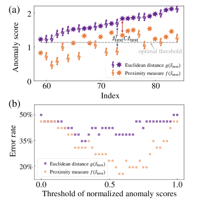
Figure 3: Anomaly detection by the methods of Euclidean distance $g\left(\vec{z}_{\rm test}\right)$ and proximity measure $f\left(\vec{z}_{\rm test}\right)$. Here, the music notes and stars represent normal samples (violin) and anomaly samples (non-violin), respectively. (a) Anomaly scores provided by different methods. The samples are sorted in ascending order of $g\left(\vec{z}_{\rm test}\right)$. (b) The error rate of different methods. The threshold is scanned within the range of anomaly scores in (a), after the range is normalized to $[0,1]$.

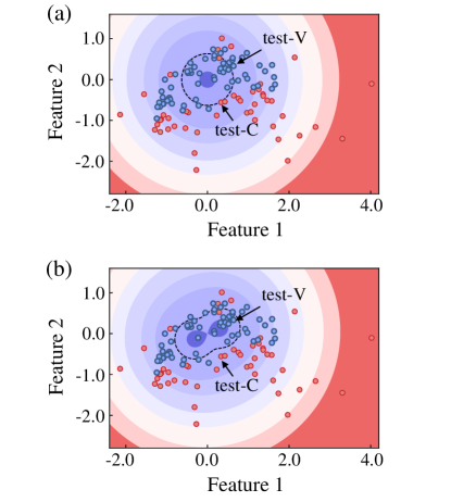
Figure 4: The spatial distribution of (a) proximity measure and (b) Euclidean distance in the feature space. Areas in red have a higher probability to be anomaly, when areas in blue are more likely to be normal. Proximity measure gives a peanut-shaped boundary line which fits better with the distribution of the normal samples.

The spatial distribution of the proximity measure in the feature space can be read out through a series of additional experiments which perform measurements after the process of training-data encoding. Instead of introducing the information of test samples, the covariance matrix of the training data is reconstructed by applying quantum tomography on the electron spin. The experimental reconstructed density matrix reads as

$$\rho_{\mathrm{exp}}=\left(\begin{array}[]{cc}0.6996&0.2151\\ 0.2151&0.3004\end{array}\right),$$ (10)

which matches the theoretical expectation $\rho_{\mathrm{cov}}$ with fidelity $F(\rho_{\mathrm{exp}},\rho_{\mathrm{cov}})=\mathrm{\textbf{tr}}\sqrt{\sqrt{\rho_{\mathrm{exp}}}\rho_{\mathrm{cov}}\sqrt{\rho_{\mathrm{exp}}}}=99\%$. For any point in the feature space $\vec{v}=(\rm{feature1,feature2})$, the proximity measure of it is estimated as $f\left(\vec{v}\right)=\left|\vec{v}\right|^{2}-\mathrm{\textbf{tr}}C\ \langle\psi_{v}|\rho_{\mathrm{exp}}|\psi_{v}\rangle$. Then the value of proximity measure is shown in Fig. 4(b) represented by different colors in the feature space, while the value of Euclidean distance is shown in Fig. 4(a). The lines dividing the neighboring areas describe how the vectors of similar anomaly scores distribute in the feature space. In the figure of proximity measure, the peanut-shaped boundary line shows that it can better learn the distribution of the normal data (blue) than using Euclidean distance. In the direction where the training samples are widely distributed, the proximity measure $f\left(\vec{z}_{\rm test}\right)$ rises slowly with the distance from the centroid. For example, while test-V is further from the centroid than test-C (Fig. 4(a)), it has a lower proximity measure than test-C (Fig. 4(b)). This indicates that it is less likely to be an anomaly sample, which is in accordance with the label of it in the dataset.

In conclusion, we experimentally demonstrated a quantum algorithm for anomaly detection on a three-qubit quantum processor. The algorithm uses resources logarithmic in the number and the dimension of the training samples. In the experiment, we trained the quantum machine with audio segments of violin which are labeled as normal and then estimate the anomaly score of a group of new samples. The experimental results show that the method of proximity measure used in our work has a better performance than classifying by Euclidean distance, with an error rate 55.6% lower than it. These results show that judging by proximity measure is more suitable for detecting anomalies when the training set has an anisotropic distribution in the feature space, which is rather common in the field of machine learning. Given a larger quantum processor, this algorithm has the potential to deal with more complicated problems efficiently, such as credit card fraud analysis with more high-dimension samples. Furthermore, this method can also take quantum states as input and work as a subroutine to detect anomalies in quantum devices, avoiding the computational complexity of reading out quantum states using quantum tomography or similar methods.

III Materials and Methods

Spin processor and experimental setup. We used an NV center with a proximal ¹³C nuclear spin ($A_{\parallel}^{\mathrm{C}}\approx 12.8\ \mathrm{MHz}$) and an intrinsic ¹⁴N nuclear spin ($A_{\parallel}^{\mathrm{N}}\approx-2.16\ \mathrm{MHz}$) in a [100]-oriented diamond. A solid immersion lens was fabricated on the NV center to improve the photon collection efficiency. The dephasing time of the spins are measured as $T_{2,\rm e}^{*}\approx$ 5.4 $\mu$s, $T_{2,\rm C}^{*}\approx$ 2.0 ms and $T_{2,\rm N}^{*}\approx$ 5.0 ms.

The experiment was carried out on a home-built confocal microscope at ambient conditions. The optical pumping and readout of the electron spin are realized by a continuous-wave laser at 532 nm which is gated with two acoustic-optic modulators (AOM). The laser beam was focused by an oil objective, while the fluorescence signal was collected by the same objective. An external magnetic field of 510 Gauss was applied by a permanent magnet along the symmetry axis of the NV center, so that the three-qubit system can be efficiently polarized to {$m_{\mathrm{e}}=0,m_{\mathrm{C}}=+1/2,m_{\mathrm{N}}=+1\}$ by laser pumping. An active temperature control to within 5 mK was used to increase the magnetic field stability.

The microwave signal used to control the electron spin was generated by an arbitrary waveform generator (AWG, crs1w000b, CIQTEK) in combination with a microwave generator through the I/Q modulation. The same AWG also generated the radio-frequency signal used to control the nuclear spins.

Dataset of the audio samples. The original audio waveforms are collected from Takahashi et al. (2016). We extract a 0.28-second segment from each audio, after excluding the silence segments. The calculation of Mel-frequency cepstral coefficients consists of four steps: (i) dividing the audio segment into frames, (ii) taking the Fourier transform, (iii) mapping the powers of the spectrum to Mel scale and taking the logs, and (iv) taking the discrete cosine transform. The segment of each audio sample is divided into 35 frames, and from each frame 12 cepstral coefficients are extracted. Here the length of each frame is 16 milliseconds, having 8 milliseconds overlap with adjacent frames. After this, each audio sample is processed into a 12 by 35 coefficients array.

To further obtain the feature vector in 2-dimension space, we flatten each array to a 420-dimension vector and apply principal component analysis to extract the main features. Defining the eigenvalues of the covariance matrix of the dataset as $\lambda_{k}$, the proportion of variance explained by the two principal components reaches $\sum_{k=1}^{2}\lambda_{k}/{\sum_{k=1}^{420}\lambda_{k}}=65\%$ (Fig. A1(a)). Thus, the subspace spanned by the first and the second principal components reserves most of the information after the feature extraction. The coordinates under the two principal component basis are used as the feature vector: (feature 1, feature 2) after being divided by 100 to rescale. The corresponding vectors of all training samples and the two test samples mentioned in the main text are shown in Fig. A1(b).

In the experiments, we train the quantum machine with 4 audio samples of the violin and then perform proximity measurement on 111 test samples in the dataset, with results shown in Fig. A2. All the samples are re-ordered in the ascending order of their Euclidean distance $g\left(\vec{z}_{\rm test}\right)$ from the centroid of the data. Both Euclidean distance $g\left(\vec{z}_{\rm test}\right)$ and proximity measure $f\left(\vec{z}_{\rm test}\right)$ of each test sample are shown.

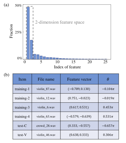
Figure A1: (a) The proportion of variance explained by each feature in the principal component analysis. The first 25 principal components are shown. (b) The 2-dimension feature vectors of all training samples and the two test samples mentioned in the main text.

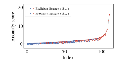
Figure A2: The anomaly scores of all the experimentally measured audio samples in the test set. The audio samples of violin are shown as blue and other types are shown as red.

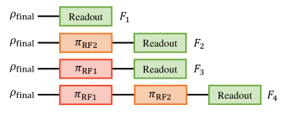
Figure A3: The readout of the possibility of electron spin at $|0\rangle_{\mathrm{e}}$. Here $\rho_{\mathrm{final}}$ is the three-qubit state to be measured. $\pi_{\mathrm{RF1}}$ and $\pi_{\mathrm{RF2}}$ represent single-qubit $\pi$ pulse on carbon spin and nitrogen spin, respectively. $F_{i}\ (i=1,2,3,4)$ is the number of photons detected in corresponding experiment.

Experimental readout method. To read out $\langle\psi_{\rm test}|\rho_{\mathrm{e}}|\psi_{\rm test}\rangle$ for each test sample, we need to measure the possibility of electron spin at $|0\rangle_{\mathrm{e}}$, denoted as $P_{0}$. In the three-qubit system, $P_{0}$ is the sum of the populations at corresponding sublevels, i.e., $P_{0}=\Sigma_{m=0}^{3}\ p_{m}$ (accordingly $P_{1}=\Sigma_{m=4}^{7}\ p_{m}$). Here, $m$ labels the binary representation of the eight energy levels (e.g. $|0\rangle=|0_{\mathrm{e}}0_{\mathrm{C}}0_{\mathrm{N}}\rangle$), and $p_{m}$ is the corresponding population. At the magnetic field of 510 Gauss, these energy levels give rise to different photon luminescence rates, leading to different detected photon numbers $N_{m}$. Thus, the number of photons detected in the experiment, denoted by $F_{1}$, is related to the distribution of populations as $F_{1}=\Sigma_{m=0}^{7}\ p_{m}N_{m}$. However, since different sets of distribution ${p_{m}}$ can produce the same $F_{1}$, one can not determine $P_{0}$ through a single readout of $F_{1}$. To overcome this, a series of experiments with different pulse sequences is required.

We apply the $\pi$ pulses shown in Fig. A3 to switch the population of different sublevels, and then count the number of photons in the new distribution. The numbers of photons detected in the four experiments give rise to the following equations

$$\left(\begin{array}[]{l}F_{1}\\ F_{2}\\ F_{3}\\ F_{4}\end{array}\right)=\left(\begin{array}[]{cccccccc}p_{0}&p_{1}&p_{2}&p_{3}&p_{4}&p_{5}&p_{6}&p_{7}\\ p_{1}&p_{0}&p_{3}&p_{2}&p_{5}&p_{4}&p_{7}&p_{6}\\ p_{2}&p_{3}&p_{0}&p_{1}&p_{6}&p_{7}&p_{4}&p_{5}\\ p_{3}&p_{2}&p_{1}&p_{0}&p_{7}&p_{6}&p_{5}&p_{4}\end{array}\right)\left(\begin{array}[]{l}N_{0}\\ N_{1}\\ N_{2}\\ N_{3}\\ N_{4}\\ N_{5}\\ N_{6}\\ N_{7}\end{array}\right).$$

The average of the photon numbers

$$\frac{F_{1}+F_{2}+F_{3}+F_{4}}{4}= P_{0}\times\frac{N_{0}+N_{1}+N_{2}+N_{3}}{4}$$

$$+P_{1}\times\frac{N_{4}+N_{5}+N_{6}+N_{7}}{4},$$

effectively averages the photon luminescence rates of different sublevels, and thus leads to the readout of $P_{0}$. Then the proximity measure of the test sample $\vec{z}_{\rm test}$ can be obtained after having $P_{0}$.

Acknowledgements.

This work is supported by the National Key R$\&$D Program of China (Grant No. 2018YFA0306600, 2017YFA0305000), the National Natural Science Foundation of China (Grants No. 11775209, 92165108, 81788101), the CAS (Grants No. GJJSTD20170001, No. QYZDY-SSW-SLH004), Anhui Provincial Natural Science Foundation, Anhui Initiative in Quantum Information Technologies (Grant No. AHY050000), the Fundamental Research Funds for the Central Universities and USTC Research Funds of the Double First-Class Initiative.

References

- Chandola et al. (2009) V. Chandola, A. Banerjee, and V. Kumar, ACM Computing Surveys 41, 1 (2009).
- Pimentel et al. (2014) M. A. Pimentel, D. A. Clifton, L. Clifton, and L. Tarassenko, Signal Processing 99, 215 (2014).
- Breunig et al. (2000) M. M. Breunig, H.-P. Kriegel, R. T. Ng, and J. Sander, in Proceedings of the 2000 ACM SIGMOD international conference on Management of data (2000) pp. 93–104.
- Hautamaki et al. (2004) V. Hautamaki, I. Karkkainen, and P. Franti, in Proceedings of the 17th International Conference on Pattern Recognition, 2004. ICPR 2004. (IEEE, Cambridge, UK, 2004) pp. 430–433 Vol.3.
- Choi (2009) Y.-S. Choi, Pattern Recognition Letters 30, 1236 (2009).
- Harrow et al. (2009) A. W. Harrow, A. Hassidim, and S. Lloyd, Physical Review Letters 103, 150502 (2009).
- Pan et al. (2014) J. Pan, Y. Cao, X. Yao, Z. Li, C. Ju, H. Chen, X. Peng, S. Kais, and J. Du, Physical Review A 89, 022313 (2014).
- Dunjko et al. (2016) V. Dunjko, J. M. Taylor, and H. J. Briegel, Physical Review Letters 117, 130501 (2016).
- Biamonte et al. (2017) J. Biamonte, P. Wittek, N. Pancotti, P. Rebentrost, N. Wiebe, and S. Lloyd, Nature 549, 195 (2017).
- Dunjko and Briegel (2018) V. Dunjko and H. J. Briegel, Reports on Progress in Physics 81, 074001 (2018).
- Schuld and Killoran (2019) M. Schuld and N. Killoran, Physical Review Letters 122, 040504 (2019).
- Lloyd et al. (2014) S. Lloyd, M. Mohseni, and P. Rebentrost, Nature Physics 10, 631 (2014).
- Li et al. (2021) Z. Li, Z. Chai, Y. Guo, W. Ji, M. Wang, F. Shi, Y. Wang, S. Lloyd, and J. Du, Science Advances 7, eabg2589 (2021).
- Rebentrost et al. (2014) P. Rebentrost, M. Mohseni, and S. Lloyd, Physical Review Letters 113, 130503 (2014).
- Li et al. (2015) Z. Li, X. Liu, N. Xu, and J. Du, Physical Review Letters 114, 140504 (2015).
- Lloyd and Weedbrook (2018) S. Lloyd and C. Weedbrook, Physical Review Letters 121, 040502 (2018).
- Hu et al. (2019) L. Hu, S.-H. Wu, W. Cai, Y. Ma, X. Mu, Y. Xu, H. Wang, Y. Song, D.-L. Deng, C.-L. Zou, and L. Sun, Science Advances 5, eaav2761 (2019).
- Huang et al. (2021) H.-L. Huang, Y. Du, M. Gong, Y. Zhao, Y. Wu, C. Wang, S. Li, F. Liang, J. Lin, Y. Xu, R. Yang, T. Liu, M.-H. Hsieh, H. Deng, H. Rong, C.-Z. Peng, C.-Y. Lu, Y.-A. Chen, D. Tao, X. Zhu, and J.-W. Pan, Physical Review Applied 16, 024051 (2021).
- Liu and Rebentrost (2018) N. Liu and P. Rebentrost, Physical Review A 97, 042315 (2018).
- Liang et al. (2019) J.-M. Liang, S.-Q. Shen, M. Li, and L. Li, Physical Review A 99, 052310 (2019).
- Herr et al. (2021) D. Herr, B. Obert, and M. Rosenkranz, Quantum Science and Technology 6, 045004 (2021).
- Kottmann et al. (2021) K. Kottmann, F. Metz, J. Fraxanet, and N. Baldelli, Physical Review Research 3, 043184 (2021).
- Hodge and Austin (2004) V. Hodge and J. Austin, Artificial Intelligence Review 22, 85 (2004).
- Giovannetti et al. (2008) V. Giovannetti, S. Lloyd, and L. Maccone, Physical Review Letters 100, 160501 (2008).
- Buhrman et al. (2001) H. Buhrman, R. Cleve, J. Watrous, and R. de Wolf, Physical Review Letters 87, 167902 (2001).
- Takahashi et al. (2016) N. Takahashi, M. Gygli, B. Pfister, and L. V. Gool (2016) pp. 2982–2986.
- Sahidullah and Saha (2012) M. Sahidullah and G. Saha, Speech Communication 54, 543 (2012).
- Müller (2007) M. Müller, Information retrieval for music and motion (Springer, New York, 2007) oCLC: ocn172976996.
- Neumann et al. (2010) P. Neumann, J. Beck, M. Steiner, F. Rempp, H. Fedder, P. R. Hemmer, J. Wrachtrup, and F. Jelezko, Science 329, 542 (2010).
- Robledo et al. (2011) L. Robledo, L. Childress, H. Bernien, B. Hensen, P. F. A. Alkemade, and R. Hanson, Nature 477, 574 (2011).
- Dolde et al. (2013) F. Dolde, I. Jakobi, B. Naydenov, N. Zhao, S. Pezzagna, C. Trautmann, J. Meijer, P. Neumann, F. Jelezko, and J. Wrachtrup, Nature Physics 9, 139 (2013).
- Dolde et al. (2014) F. Dolde, V. Bergholm, Y. Wang, I. Jakobi, B. Naydenov, S. Pezzagna, J. Meijer, F. Jelezko, P. Neumann, T. Schulte-Herbrüggen, J. Biamonte, and J. Wrachtrup, Nature Communications 5, 3371 (2014).
- Rong et al. (2015) X. Rong, J. Geng, F. Shi, Y. Liu, K. Xu, W. Ma, F. Kong, Z. Jiang, Y. Wu, and J. Du, Nature Communications 6, 8748 (2015).
- Zhang et al. (2021) Q. Zhang, Y. Guo, W. Ji, M. Wang, J. Yin, F. Kong, Y. Lin, C. Yin, F. Shi, Y. Wang, and J. Du, Nature Communications 12, 1529 (2021).
- Maurer et al. (2012) P. C. Maurer, G. Kucsko, C. Latta, L. Jiang, N. Y. Yao, S. D. Bennett, F. Pastawski, D. Hunger, N. Chisholm, M. Markham, D. J. Twitchen, J. I. Cirac, and M. D. Lukin, Science 336, 1283 (2012).
- Yang et al. (2016) S. Yang, Y. Wang, D. D. B. Rao, T. Hien Tran, A. S. Momenzadeh, M. Markham, D. J. Twitchen, P. Wang, W. Yang, R. Stöhr, P. Neumann, H. Kosaka, and J. Wrachtrup, Nature Photonics 10, 507 (2016).
- Bradley et al. (2019) C. Bradley, J. Randall, M. Abobeih, R. Berrevoets, M. Degen, M. Bakker, M. Markham, D. Twitchen, and T. Taminiau, Physical Review X 9, 031045 (2019).
- Jacques et al. (2009) V. Jacques, P. Neumann, J. Beck, M. Markham, D. Twitchen, J. Meijer, F. Kaiser, G. Balasubramanian, F. Jelezko, and J. Wrachtrup, Physical Review Letters 102, 057403 (2009).
- Waldherr et al. (2014) G. Waldherr, Y. Wang, S. Zaiser, M. Jamali, T. Schulte-Herbrüggen, H. Abe, T. Ohshima, J. Isoya, J. F. Du, P. Neumann, and J. Wrachtrup, Nature 506, 204 (2014).