HoneyTop90: A 90-line MATLAB code for topology optimization using honeycomb tessellation

  Abstract: This paper provides a simple, compact and efficient 90-line pedagogical MATLAB code for topology optimization using hexagonal elements (honeycomb tessellation). Hexagonal elements provide nonsingular connectivity between two juxtaposed elements and, thus, subdue checkerboard patterns and point connections inherently from the optimized designs. A novel approach to generate honeycomb tessellation is proposed. The element connectivity matrix and corresponding nodal coordinates array are determined in 5 (7) and 4 (6) lines, respectively. Two additional lines for the meshgrid generation are required for an even number of elements in the vertical direction. The code takes a fraction of a second to generate meshgrid information for the millions of hexagonal elements. Wachspress shape functions are employed for the finite element analysis, and compliance minimization is performed using the optimality criteria method. The provided Matlab code and its extensions are explained in detail. Options to run the optimization with and without filtering techniques are provided. Steps to include different boundary conditions, multiple load cases, active and passive regions, and a Heaviside projection filter are also discussed. The code is provided in Appendix A, and it can also be downloaded along with supplementary materials from https://github.com/PrabhatIn/HoneyTop90.

Keywords: Topology optimization; Hexagonal elements; MATLAB; Wachspress shape functions; Compliance minimization

 

1 Introduction

Topology optimization (TO), a design technique, determines an optimized material distribution within a specified design domain with known boundary conditions by extremizing an objective for the given physical and geometrical constraints (Sigmund and Maute, 2013). In a typical continuum optimization setting, the design domain is parameterized by either quadrilateral or polygonal finite elements (FEs), and the associated boundary value problems are solved. Each FE is assigned a design variable $\rho\in[0,\,1]$. $\rho=1$ and $\rho=0$ indicate the solid and the void states of the element respectively.

There exist numerous pedagogical TO MATLAB codes online in Sigmund (2001); Suresh (2010); Challis (2010); Huang and Xie (2010); Andreassen et al. (2011); Saxena (2011); Talischi et al. (2012b); Wei et al. (2018); Ferrari and Sigmund (2020); Picelli et al. (2020) that can help a user to learn and explore various optimization techniques. In addition, one may refer to the articles by Han et al. (2021a); Wang et al. (2021) for a comprehensive discussion on various TO educational codes. A simple, compact and efficient educational code using pure (regular) hexagonal finite elements (honeycomb tessellation) with Wachspress shape functions however cannot be found in the current state-of-the-art of TO. Such codes can find importance for newcomer students to learn, explore, realize and visualize the characteristics of hexagonal FEs in a TO framework with a minimum effort. Honeycomb tessellation offers nonsingular geometric connectivity and thus, circumvents checkerboard patterns and single-point connections inherently from the optimized designs (Saxena and Saxena, 2003, 2007; Langelaar, 2007; Talischi et al., 2009; Saxena, 2011; Kumar, 2017). In addition, as per Sukumar and Tabarraei (2004), polygonal/hexagonal FEs provide better accuracy in numerical solutions and are suitable for modeling of polycrystalline materials.

An approach with hexagonal FEs is presented by Saxena (2011), and the author also shares the related MATLAB code. However, a new reader may not find the code generic primarily because it does not detail how to generate the honeycomb tessellation for a given problem. Talischi et al. (2012a) provide a MATLAB code to generate polygonal mesh using implicit description of the domain and the centroidal Voronoi diagrams. The code is suitable to parameterize arbitrary geometrical shapes using polygonal elements, however it requires many subroutines and involved processes and thus, a newcomer may find difficulties to learn and explore with that code. Talischi et al. (2012b) use the polygonal meshing method (Talischi et al., 2012a) in their TO approach. TO approaches using the polymesher code (Talischi et al., 2012a) can also be found in Sanders et al. (2018); Giraldo-Londoño and Paulino (2021). The motif herein is to provide a simple, compact, efficient and hands-on pedagogical MATLAB code with hexagonal elements such that a user can readily: (A) generate hexagonal FEs, (B) obtain the corresponding element connectivity matrix and nodal coordinates array and (C) perform FE analysis and TO and also, visualize the intermediate design evolution of the optimization in line with (Andreassen et al., 2011; Ferrari and Sigmund, 2020). (A) is expected to significantly reduce the learning time for newcomers in TO using honeycomb tessellation, while this in association with (B) can also be used to solve various design problems wherein explicit information of the element connectivity matrix and nodal coordinates array are required, e.g., problems involving finite deformation (Saxena and Sauer, 2013; Kumar et al., 2016, 2017, 2019, 2021), linear elasticity-based problems, e.g., in Sukumar and Tabarraei (2004); Tabarraei and Sukumar (2006); Kumar and Saxena (2015); Singh et al. (2020) and related references therein, etc. In addition, the TO approaches based on element design variables can be readily implemented and studied as the presented code provides uniform hexagonal tessellations.

In summary, the primary goals of this paper are to provide a simple and efficient way to generate honeycomb tessellation, TO with/without commonly used filtering techniques and optimality criteria approach, steps to include various design problems, and explicit expressions for the Wachspress shape functions and elemental stiffness matrix for the benefits of new students to explore, learn and realize TO with hexagonal elements in relatively less time. In addition, one can extend the presented code for advanced optimization problems involving stress and buckling constraints.

The remainder of the paper is organized as follows. Sec. 2 briefly describes the compliance minimization TO problem formulation with volume constraints, optimality criteria updating, sensitivity filtering and density filtering schemes for the sake of completeness. Sec. 3 provides a novel, compact and efficient way to generate element connectivity matrix and the corresponding nodal coordinates array for a honeycomb tessellations. In addition, finite element analysis, filtering and optimization procedures are also described, and results of the Messerschmitt-Bolkow-Blohm (MBB) beam are presented with and without filtering schemes. Further, to demonstrate distinctive features of the hexagonal elements, numerical examples for the beam design are presented, and results are compared with those obtained using quadrilateral elements. Sec. 4 presents the extensions of the code towards–different boundary conditions, multiloads situations, non-designs (passive) domains, and a Heaviside projection filtering scheme. In addition, directions for various other extensions are also reported. Lastly, conclusions are drawn in Sec. 5.

2 Problem formulation

We consider the MBB beam design problem to demonstrate the presented Matlab TO code. Compliance of the beam is minimized for a given volume (resource) constraint. A symmetric half design domain of the beam with the pertinent boundary conditions and external load $\mathbf{F}$ is depicted in Fig. 1. $L_{x}$ and $L_{y}$ indicate dimensions in $x-$ and $y-$directions respectively herein and henceforth.

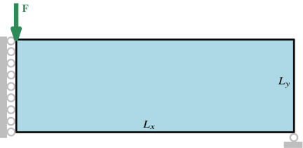
Figure 1: A symmetric MBB beam design domain with boundary conditions and an external force, $\mathbf{F}$

The design domain is parameterized using Nelem hexagonal FEs represented via $\Omega_{j}^{\text{H}}|_{j=1,\,2,\,3,\,\cdots,\,\texttt{Nelem}}$. Each FE is assigned a design variable $\rho_{j}\in[0,\,1]$ that is constant within the element (Sigmund, 2007). The stiffness matrix of element $j$ is determined as

$$\mathbf{k}_{j}=E(\rho_{j})\mathbf{k}_{0}=\left(E_{\text{min}}+\rho_{j}^{p}\left(E_{0}-E_{\text{min}}\right)\right)\mathbf{k}_{0},$$ (1)

where $E(\rho_{j})$, Young’s modulus of element $j$, is evaluated using the modified Solid Isotropic Material with Penalization (SIMP) formulation (Sigmund, 2007). $E_{0}$ indicates the Young’s modulus of a solid element ($\rho_{j}=1$) and that of a void element ($\rho_{j}=0$) is denoted via $E_{\text{min}}$. Material contrast i.e. $\frac{E_{\text{min}}}{E_{0}}=10^{-9}$ is fixed to ensure nonsingular global stiffness matrix $\mathbf{K}$ (Sigmund, 2001). $\mathbf{k}_{0}$ is the element stiffness matrix with $E(\rho_{j})=1$. The SIMP parameter $p$ is set to 3 in this paper.

The following optimization problem is solved:

$$\left.\begin{aligned} \hfil\displaystyle\begin{split}&{\min_{\bm{\rho}}}\quad C({\bm{\rho}})=\mathbf{u}^{\top}\mathbf{K}(\bm{\rho})\mathbf{u}=\sum_{j=1}^{\mathtt{Nelem}}\mathbf{u}_{j}^{\top}\mathbf{k}_{j}(\rho_{j})\mathbf{u}_{j}\\ &\text{subjected to:}\\ &\bm{\lambda}:\,\,\mathbf{K}\mathbf{u}-\mathbf{F}=\mathbf{0}\\ &\Lambda:\,\,\text{g}=\frac{V(\bm{\rho})}{\mathtt{Nelem}\,V^{*}_{f}}-1=\frac{\sum_{j=1}^{\mathtt{Nelem}}v_{j}\rho_{j}}{\mathtt{Nelem}\,V^{*}_{f}}-1\leq 0\\ &\quad\,\,\,\,\bm{0}\leq\bm{\rho}\leq\bm{1}\\ &\text{Data:}\quad\mathbf{F},\,V^{*},\,V^{*}_{f},\,v_{j}(=1),\,E_{0},\,E_{\text{min}},\,p\end{split}\end{aligned}\right\},$$ (2)

where $C({\bm{\rho}})$ represents the compliance, $\mathbf{u}$ and $\mathbf{F}$ indicate the global displacement and force vectors respectively, and $\mathbf{u}_{j}$ is the displacement vector corresponding to element $j$. $V$ is the total material volume, and $V^{*}_{f}$ is the permitted resource volume fraction of the design domain. $\bm{\rho}$, the design vector, is constituted via $\rho_{j}$. $\bm{\lambda}$ (vector) and $\Lambda$ (scalar) are the Lagrange multipliers corresponding to the state equilibrium equation and the volume constraint respectively. $\bm{\lambda=-2\mathbf{U}}$ can be found using the adjoint-variable method (see Appendix B). Sensitivities of the objective with respect to $\rho_{j}$ using $\bm{\lambda}$ and (1) can be determined as (Appendix B)

$$\frac{\partial C}{\partial\rho_{j}}=-\mathbf{u}_{j}^{\top}\frac{\partial\mathbf{k}_{j}}{\partial\rho_{j}}\mathbf{u}_{j}=-p(E_{0}-E_{\text{min}})\rho_{j}^{p-1}\mathbf{u}_{j}^{\top}\mathbf{k}_{0}\mathbf{u}_{j}.$$ (3)

Likewise, derivatives of the volume constraint with respect to $\rho_{j}$ are determined as

$$\frac{\partial\text{g}}{\partial\rho_{j}}=\frac{v_{j}}{\mathtt{Nelem}\,V^{*}_{f}}=\frac{1}{\mathtt{Nelem}\,V^{*}_{f}},$$ (4)

wherein $v_{j}=1$ is assumed. The optimization problem (2) is solved using the standard optimality criteria method wherein the design variables are updated per Sigmund (2001) given as

$$\rho_{j}^{k+1}=\left\{\begin{aligned} \hfil\displaystyle\begin{split}&{(\rho_{j}^{k})}_{-}\qquad\text{if}\,\mathcal{M}_{j}^{k}<{(\rho_{j}^{k})}_{-},\\ &{(\rho_{j}^{k})}_{+}\qquad\text{if}\,\mathcal{M}_{j}^{k}>{(\rho_{j}^{k})}_{+},\\ &\mathcal{M}_{j}^{k}\qquad\,\,\,\,\text{otherwise},\end{split}\end{aligned}\right.$$ (5)

where ${(\rho_{j}^{k})}_{-}=\max(0,\,\rho_{j}^{k}-m)$, ${(\rho_{j}^{k})}_{+}=\min(1,\,\rho_{j}^{k}+m)$, and $m\in[0,\,1]$ indicates the move limit. $\mathcal{M}_{j}^{k}=\rho_{j}^{k}{\left(\frac{-\frac{\partial C}{\partial\rho_{j}}}{\Lambda_{k}\frac{\partial\text{g}}{\partial\rho_{j}}}\right)}^{\frac{1}{2}}$, where $\Lambda_{k}$ is the value of $\Lambda$ at the $k^{\text{th}}$ iteration. The final value of $\Lambda$ is determined using the bisection algorithm (Sigmund, 2001).

We solve the optimization problem (2) with and without filtering techniques. Mesh-independent density filtering (Bruns and Tortorelli, 2001; Bourdin, 2001) and sensitivity filtering (Sigmund, 1997, 2001) are considered. As per the density filtering (Bruns and Tortorelli, 2001; Xu et al., 2020), the filtered density $\bar{\rho_{j}}$ of element $j$ is evaluated as

$$\tilde{\rho_{j}}=\frac{\displaystyle\sum_{i\in n_{j}}v_{i}\rho_{i}w(\mathbf{x}_{i})}{\displaystyle\sum_{i\in n_{j}}v_{i}w(\mathbf{x}_{i})},$$ (6)

where $v_{i}$ and $\rho_{i}$ are the volume and material density of the $i^{\text{th}}$ neighboring element respectively, and $n_{j}$ is the total number of neighboring elements of element $j$ within a circle of radius $r_{\text{fill}}$. $w(\mathbf{x}_{j})$, a linearly decaying weight function, is defined as (Bruns and Tortorelli, 2001; Bourdin, 2001; Han et al., 2021b)

$$w(\mathbf{x}_{i})=\max\left(0,\frac{||\mathbf{x}_{i}-\mathbf{x}_{j}||}{r_{\text{fill}}}\right),$$ (7)

$\mathbf{x}_{i}$ and $\mathbf{x}_{j}$ are the center coordinates of the $i^{\text{th}}$ and $j^{\text{th}}$ elements respectively, and $||.||$ defines a Euclidean distance. The chain rule is used to evaluate the final sensitivities of a function $f$ with respect to ${\rho_{j}}$. With the sensitivity filter, the filtered sensitivities are evaluated as (Sigmund, 1997)

$$\frac{\overline{\partial C}}{\partial\rho_{j}}=\frac{\displaystyle\sum_{i\in n_{j}}w(\mathbf{x}_{i})\rho_{i}\frac{\partial C}{\partial\rho_{i}}}{\max(\delta,\,\rho_{j})\displaystyle\sum_{i\in n_{j}}w(\mathbf{x}_{i})},$$ (8)

where $\delta$, a small positive number, is set to $10^{-3}$ for avoiding division by zero (Andreassen et al., 2011).

3 Implementation detail

In this section, MATLAB implementation of HoneyTop90 is presented in detail. We first provide a novel, efficient and simple code to generate honeycomb elements connectivity matrix and corresponding nodal coordinates array in just 9 (13) lines. Thereafter, finite element analysis, filtering and optimization are described for the presented HoneyTop90 TO code. The MBB beam is optimized herein to demonstrate HoneyTop90.

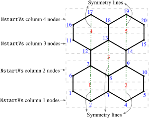
Figure 2: A schematic diagram for element and node numbering steps. Texts in blue and red indicate node and element numbers respectively, and henceforth the same colors are used to indicate nodes and elements. NstartVs is determined on the line 6 of the HoneyTop90 code (Appendix A).

3.1 Element connectivity and nodal coordinates matrices (lines 5-18)

Let $\mathtt{HNex}$ and $\mathtt{HNey}$ be the number of hexagonal elements in $x-$ and $y-$directions respectively. Each element consists of six nodes, and each node possesses two degrees of freedom (DOFs). For element $i$, DOFs $2i-1$ and $2i$ correspond respectively to the displacement in $x-$ and $y-$directions. In the provided code (Appendix A), the element DOFs matrix HoneyDOFs is generated on lines 6-10, and the corresponding nodal coordinate matrix HoneyNCO is generated on lines 11-14. When $\mathtt{HNey}$ is an even number, corresponding HoneyDOFs and HoneyNCO are updated on lines 15-18. The $i^{\text{th}}$ row of HoneyDOFs gives DOFs corresponding to element $i$, whereas that of HoneyNCO contains $x-$ and $y-$coordinates of node $i$.

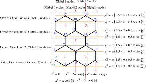
Figure 3: Finding the nodal coordinates of a honeycomb tessellation. $\mathbf{O}$ is the origin.

Columns of the matrix NstartVs indicate node numbers of FEs starting from the bottom to top rows (Fig. 2). The first $x-$DOFs of both symmetrical half quadrilaterals (see Fig. 2) of each hexagonal FE are stored in the matrix DOFstartVs. DOFs of all such quadrilaterals are recorded in the matrix NodeDOFs. The redundant rows of the matrix NodeDOFs are removed using setdiff MATLAB function, and the remaining DOFs are noted in the matrix ActualDOFs. The final honeycomb DOFs connectivity matrix HoneyDOFs is obtained from the matrix ActualDOFs and recorded on line 10.

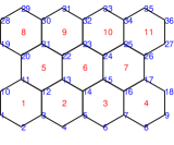
(a) $\mathtt{HNex}=4,\,\mathtt{HNey}=3$

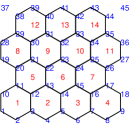
(b) $\mathtt{HNex}=4,\,\mathtt{HNey}=4$. 37 and 45 are the hanging nodes.

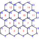
(c) $\mathtt{HNex}=4,\,\mathtt{HNey}=4$. Hanging nodes are removed (lines 15-18) and node numbering is updated.

Figure 4: Different honeycomb tessellations. Hanging nodes are detected in (4(b)), which are removed, and the updated node numbers with respective elements are plotted in (4(c)).

Coordinates of vertex $m|_{m=0,\,1,\,\cdots,\,6}$ of a hexagonal element with centroid (a local coordinate system) at the origin can be written as $\left(a\cos(\frac{(2m-1)\pi}{6},\,a\sin(\frac{(2m-1)\pi}{6})\right)$, where $a$ is the length of an edge, which can have different values as desired. When the origin is shifted to ($-a\cos(\frac{\pi}{6}),\,-0.75a$) with respect to the local coordinate system of element 1 (Fig. 3), the $y-$coordinates of the vertices for a honeycomb tessellation can be written as (Fig. 3)

$$\begin{split}y_{k}^{l}=a\left(1.5l+\frac{(-1)^{k}}{2}\sin\left(\frac{\pi}{6}\right)\right),\\ \text{with}\,k=1,\,2;\,l=0,\,1,\,\cdots,\,\texttt{HNey}\end{split}$$ (9)

Likewise, the $x-$coordinates can be written as (Fig. 3)

$$x^{n}=na\cos\left(\frac{\pi}{6}\right),\text{with}\,n=0,\,1,\,\cdots,\,\texttt{2HNex}$$ (10)

In view of (9), the $y-$coordinates of the nodes for a general honeycomb tessellation, i.e., corresponding to the matrix HoneyDOFs, are determined on lines 11-13 and stored in the vector Ncyf. With the $x-$coordinates (10), the matrix HoneyNCO records the nodal coordinates of the meshgrid on line 14, wherein $x-$ and $y-$coordinates are kept in the first and second columns respectively. In the provided code (Appendix A), $a$ is taken $1/\sqrt{3}$ (lines 14 and 43). For the desired edge length $\kappa$, the user should replace $1$ with $\kappa$ on lines 14 and 43 (centroid determination) of HoneyTop90 code and may have to accordingly determine the shape functions and the elemental stiffness matrix.

When $\mathtt{HNey}$ is an even number, hanging nodes are observed (Fig. 4(b)) with the above presented steps. Hanging nodes are removed (lines 15-18), and the connectivity DOFs matrix HoneyDOFs is updated on line 16 accordingly. Likewise, HoneyNCO is updated on line 17 by removing the hanging nodes (Fig. 4(b)). One notices that the DOFs and nodal coordinates matrices are determined primarily by using reshape and repmat MATLAB functions. The former rearranges the given matrix for the specified number of rows and columns consistently, whereas the latter duplicates the matrix for the assigned number of times along the $x-$ and $y-$directions. The obtained element connectivity matrices for Fig. 4(a) and Fig. 4(c) are noted below in the matrices $\texttt{HoneyDOFs}_{4\times 3}$ (11) and $\texttt{HoneyDOFs}_{4\times 4}$ (12) respectively. Entries in row $i|_{i=1,\,2\,\cdots,\,\mathtt{Nelem}}$ of these matrices indicate DOFs corresponding to element $i$. One can determine honeycomb element connectivity matrix $\mathtt{HoneyElem}$ from the HoneyDOFs as,

⬇

HoneyElem = HoneyDOFs(:,2:2:end)/2.

The $r^{\text{th}}$ row of the matrix HoneyElem contains nodes in the counter-clockwise sense that constitute element $r$. HoneyNCO and HoneyElem provide an important set of ingredients for performing finite element analysis using hexagonal FEs. The following code can be used to plot and visualize the honeycomb tessellation generated by the steps mentioned above (lines 6-18).

⬇

% Code to plot honeycomb tessellation

H = figure(1);set(H,’color’,’w’);

X = reshape(HoneyNCO(HoneycombElem’,1),6,Nelem);

Y = reshape(HoneyNCO(HoneycombElem’,2),6,Nelem);

patch(X, Y,’w’,’EdgeColor’,’k’);axis off equal;

The MBB beam (Fig. 1) is meshed using $48\times 16$ and $57\times 19$ hexagonal elements to illustrate the discretization part of HoneyTop90 (Fig. 5). Note that instead of removing hanging nodes as described above, one can also use those nodes to close the rectangular domain by forming triangular and quadrilateral elements at the boundaries. However, the computational cost of the entire optimization process can increase. This may happen partly due to the requirement of different bookkeeping to store the element connectivity and stiffness matrices of hexagonal, quadrilateral and triangular elements and partly because, with different element types, nodal design variable-based TO methods need to be employed instead of elemental design variable-based TO approaches.

Next, the computation time taken by the code to generate HoneyDOFs and HoneyNCO for different meshgrids is noted in Table 1. It can be observed that the DOFs connectivity matrix and corresponding nodal coordinates array for $3000\times 1000$ FEs can be generated within a fraction of a second.

$$\texttt{HoneyDOFs}_{4\times 3}=\setcounter{MaxMatrixCols}{12}\begin{bmatrix}23&24&21&22&19&20&1&2&3&4&5&6\\ 27&28&25&26&23&24&5&6&7&8&9&10\\ 31&32&29&30&27&28&9&10&11&12&13&14\\ \vdots&\vdots&\vdots&\vdots&\vdots&\vdots&\vdots&\vdots&\vdots&\vdots&\vdots&\vdots\\ 71&72&69&70&67&68&49&50&51&52&53&54\end{bmatrix}$$ (11)

$$\texttt{HoneyDOFs}_{4\times 4}=\setcounter{MaxMatrixCols}{12}\begin{bmatrix}23&24&21&22&19&20&1&2&3&4&5&6\\ 27&28&25&26&23&24&5&6&7&8&9&10\\ 31&32&29&30&27&28&9&10&11&12&13&14\\ \vdots&\vdots&\vdots&\vdots&\vdots&\vdots&\vdots&\vdots&\vdots&\vdots&\vdots&\vdots\\ 87&88&85&86&83&84&65&66&67&68&69&70\end{bmatrix}$$ (12)

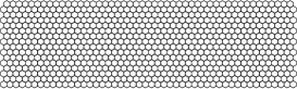
(a) $48\times 16$ hexagonal elements

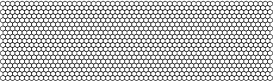
(b) $57\times 19$ hexagonal elements

Figure 5: Honeycomb tessellations for the MBB beam.

Table 1: Computation time required to generate different mesh sizes. A 64-bit operating system machine with 8.0 GB RAM, Intel(R), Core(TM) i5-8265U CPU 1.60 GHz is used.

Mesh Size ($\mathtt{HNex}\times\mathtt{HNey}$)	Computation time (s)
	HoneyDOFs	HoneyNCO
$100\times 50$	0.031	0.0022
$250\times 125$	0.037	0.0025
$500\times 250$	0.066	0.011
$1000\times 500$	0.156	0.032
$2000\times 1000$	0.553	0.135
$3000\times 1000$	0.753	0.178

3.2 Finite element analysis (lines 20-38 and lines 60-62)

Nelem and $\mathtt{Nnode}$ (the total number of nodes) for the current meshgrid are determined using $\mathtt{size}$ and $\mathtt{deal}$ MATLAB functions on line 19. Alternatively, one can also use the following codes to determine them:

⬇

Nelem = HNex*ceil(HNey/2) + (HNex-1)*floor(HNey/2);

if(mod(HNey,2)==0)

Nnode = (2*HNex+1)*(HNey+1)-2; % When HNey is an even

else

Nnode = (2*HNex+1)*(HNey+1); % When HNey is an odd

end

The total DOFs is listed in alldof on line 23. The material Young’s modulus $E_{0}$ and that of a void element $E_{\text{min}}$ are respectively denoted by $\mathtt{E0}$ and $\mathtt{E\text{min}}$. The Poisson’s ratio $\nu=0.29$ is considered. The elemental stiffness matrix  Ke is mentioned on lines 27-38 that is evaluated using the Wachspress shape functions (Wachspress, 1975) with plane stress assumptions. Talischi et al. (2009) also employ these shape functions (see Appendix C and Appendix D). However, a method to generate honeycomb tessellation which is not so straightforward, steps to include various problems, explicit expressions for the shape functions and a MATLAB code to learn and extend the method are not presented in Talischi et al. (2009).

The global stiffness matrix $\mathtt{K}$ is evaluated on line 61 using the sparse function. The rows and columns of the matrix HoneyDOFs are recorded in vector iK and jk respectively (Andreassen et al., 2011). Boundary conditions of the given design description are recorded in the vector fixeddofs on line 22, and the applied external force is noted in the vector F on line 20. The vectors fixeddofs and F can be modified based on the different problem settings. The displacement vector U is determined on line 62.

3.3 Filtering, Optimization and Results Printing (lines 39-52 and lines 63-89)

We provide three filtering cases for a problem—sensitivity filtering (ft = 1), density filtering (ft=2) and null (no) filtering (ft =0). The latter is included to demonstrate the characteristics of hexagonal elements in view of checkerboard patterns and point connections. For generating the required filter matrices (DD and HHs, lines 44-52), we need the coordinates of centroids of the hexagonal elements. For that, the center coordinates array ct is determined on lines 40-43. The $i^{\text{th}}$ row of ct gives $x-$ and $y-$coordinates of the centroid of element $i$. ct matrix is used to evaluate filtering parameter and also, is employed to plot the intermediate results using the scatter MATLAB function.

The neighboring elements of each element for the given filter radius rfill are determined on line 47. They are stored in the matrix DD whose first, second and third entries indicate the neighborhood FE index, the selected element index and center-to-center distance between them, respectively. The filtering matrix HHs is evaluated on line 52 using the spdiags function (Talischi et al., 2012b). S = spdiags(Bin, d, m, n) creates an m-by-n sparse matrix S by taking the columns of Bin and placing them along the diagonals specified by d.

The given volume fraction volfrac is used herein to set the initial guess of TO. The design vector $\bm{\rho}$ is denoted by x in the code. The physical material density vector is represented by xPhys. With either $\mathtt{ft=0}$ or $\mathtt{ft=1}$, xPhys is equal to the design vector, whereas with $\mathtt{ft=2}$, xPhys is represented via the filtered density $\tilde{\bm{\rho}}$ (line 84). The optimization updation is performed on line 81 as per Ferrari and Sigmund (2020). The objective, i.e., compliance of the design is obtained on line 65. The mechanical equilibrium equation is solved to determine displacement vector U on line 62 using the decomposition function with lower triangle part of K. decomposition function provides efficient Cholesky decomposition of the global stiffness matrix, and thus, solving state equations becomes computationally cheap. The sensitivities of the objective are evaluated and stored in the vector dc on line 66. The vector dc is updated as per different $\mathtt{ft}$ values. Volume constraint sensitivities are recorded in the vector dv and updated within the loop based on chosen filtering technique. For plotting and visualizing the intermediate results evolution, we use scatter function as on line 89. The plotting function uses the centroid coordinates in conjunction with the intermediate physical design vector xPhys. Alternatively, one can also use

⬇

colormap(’gray’);

X = reshape(HoneyNCO(HoneyElem’,1),6,Nelem);

Y = reshape(HoneyNCO(HoneyElem’,2),6,Nelem);

patch(X, Y, [1-xPhys],’EdgeColor’,’k’);

axis equal off; pause(1e-6);

to plot the intermediate results.

3.4 MBB beam optimized results

HoneyTop90 MATLAB code is provided in Appendix A. The code is called as

⬇

HoneyTop90(HNex,HNey,volfrac,penal,rfill,ft);

to find the optimized beam designs for the domain and boundary conditions shown in Fig. 1. The results are obtained with and without filtering schemes, i.e., ft = 0, 1, 2 are used. volfrac, the permitted volume fraction, is set to 0.5. The SIMP parameter denoted by penal is set to 3. Three mesh sizes with $60\times 20$, $150\times 50$ and $300\times 100$ FEs are considered. The filter radius rfill is set to 0.03 times the length of the beam domain, i.e., $1.8\sqrt{3}$, $4.5\sqrt{3}$ and $9\sqrt{3}$ for the $60\times 20$, $150\times 50$ and $300\times 100$ FEs respectively.

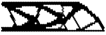
(a) $C=298.70$

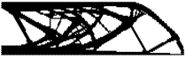
(b) $C=290.47$

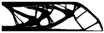
(c) $C=282.49$

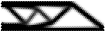
(d) $C=307.93$

(e) $C=309.54$

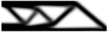
(f) $C=302.33$

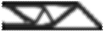
(g) $C=337.44$

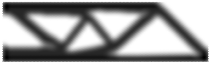
(h) $C=358.63$

(i) $C=367.64$

Figure 6: The optimized MBB beam designs are displayed. The results with corresponding compliance $C$ depicted in the first (6(a)-6(c)), second (6(d)-6(f)) and third (6(g)-6(i)) rows are obtained with no filtering, sensitivity filtering and density filtering respectively.

The optimized results obtained with different filtering approaches are displayed in Fig. 6. The results with ft=0 (Fig. 6(a)-6(c)) are free from checkerboard patterns and are the best performing ones. They are however mesh dependent and contain thin members as expected. Therefore, to circumvent such features one can use either filtering or length scale constraints, e.g., perimeter constraint (Haber et al., 1996). Results displayed in the second (Fig. 6(d)-6(f)) and third (Fig. 6(g)-6(i)) rows are obtained with sensitivity filtering (ft=1) and density filtering (ft=2) respectively. These designs do not have checkerboard patterns and also, they are mesh independent, i.e., they have same topology irrespective of the mesh sizes employed. In addition, obtained topologies with sensitivity filtering and density filtering are same herein but that may not be the case always since both filters work on different principles as noted in Sec. 2. Figure 8 depicts the objective convergence plots for the MBB beam design for 200 OC iterations. One can note that objective history plots are stable and have converging nature.

(a) $60\times 20$ FEs

(b) $150\times 50$ FEs

(c) $300\times 100$ FEs

Figure 8: Objective convergence plots of the MBB beam for 200 optimality criteria (OC) iterations.

3.4.1 Checkerboard-patterns-free designs

In this section, the results obtained with hexagonal elements are compared with the corresponding quadrilateral FEs. The 88-line code, top88 (Andreassen et al., 2011), is employed to generate the results with quadrilateral FEs. Filtering techniques are not used. The volume fraction is set to 0.5 and the SIMP parameter $p=3$ is used.

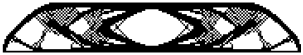
(a)

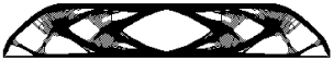
(b)

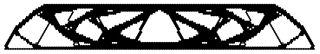
(c)

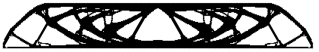
(d)

Figure 8: The optimized MBB beam designs. 8(a)-8(b) results with quadrilateral FEs (top88), and 8(c)-8(d) results are with hexagonal elements (HoneyTop90). $90\times 30$ FEs and $180\times 60$ FEs are used to generate results in the first and second columns, respectively.

Figure 8 depicts the optimized designs obtained using top88 and HoneyTop90 codes with different mesh sizes. One can note that the optimized designs obtained via quadrilateral FEs (Fig. 8a and Fig. 8b) contain checkerboard patterns, patches of the alternate void and solid FEs. However, such fine patches are not observed in the optimized design obtained via hexagonal FEs (Fig. 8c and Fig. 8d). Thus, honeycomb tessellation circumvents checkerboard patterns automatically due to its geometrical constructions, i.e., edge connections between two neighboring FEs.

4 Simple extensions

Herein, various simple extensions of the presented MATLAB code are described to solve different design problems with different input loads and boundary conditions. Heaviside projection filter scheme is also implemented in Sec. 4.4.

4.1 Michell structure

We design a Michell structure to demonstrate the code with different boundary conditions. In view of symmetry, we have only used the right half of the design domain that is depicted in Fig. 9(a). The corresponding loads and boundary conditions are also shown. To accommodate this problem in the presented code, the following changes are performed: Line 20 is altered to

⬇

F = sparse(2*1,1,-1,2*Nnode,1); % Input force

and line 22 is changed to

⬇

fixeddofs = [2*(1:2*HNex+1:(2*HNex+1)*HNey+1)-1,(2*(2*HNex+1)), (2*(2*HNex+1))-1]; % Fixed DOFs

With these above modifications, we call the code as

⬇

HoneyTop90(120,120,0.20,3,3.6*sqrt(3),ft);

and the obtained final designs are depicted in Fig. 9 for different ft values. One notices that optimization with ft=0 (Fig. 9(b)) gives a checkerboard free optimized designs, however thin members can be seen as also noted earlier. The obtained optimized designs with ft=2 (Fig. 9(c)) and ft=3 (Fig. 9(d)) have different topologies. This is because, sensitivity filter (ft=2) and density filter (ft=3) have different definition (see (6) and (8)). Optimized design obtained with ft=0 is the best performing structure, and that with ft=3 is worst the performing continuum.

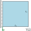
(a) Michell design domain

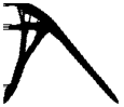
(b) $\texttt{ft = 0},\,C=58.53$

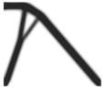
(c) $\texttt{ft = 1},\,C=59.32$

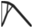
(d) $\texttt{ft = 2},\,C=83.78$

Figure 9: A symmetric half design domain for the Michell structure is shown in (9(a)). The corresponding load and boundary conditions are also depicted. Optimized results (9(b)) without filtering (9(c)) with sensitivity filter and (9(d)) with density filter are displayed.

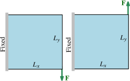
(a)

(b) $\texttt{ft = 1},\,C=86.4162$

Figure 10: Design domain for a cantilever beam with two load cases is displayed in (10(a)). The optimized design is shown in (10(b)).

4.2 Multiple loads

A cantilever beam design displayed in Fig. 10(a) (Sigmund, 2001) is solved with two load cases herein by modifying HoneyTop90 code.

As the problem involves two load cases, the input force is placed in a two-column vector. The corresponding displacement vector is determined and recorded in a two-column vector. The objective function is determined as

$$C=\displaystyle\sum_{k=1}^{2}\mathbf{U}_{k}^{\top}\mathbf{K}\mathbf{U}_{k}$$ (13)

where $\mathbf{U}_{k}$ indicates displacement for the $k^{\text{th}}$ load case. In the code, lines 20, 21 and 22 are modified to

⬇

F = sparse([(2*HNex+1)*2, 2*Nnode],[1 2],[-1 1],2*Nnode,2); % Input force

⬇

U = zeros(2*Nnode,2); % Initializing displacement vector

and

⬇

fixeddofs = [2*(1:2*HNex+1:(2*HNex+1)*HNey+1)-1,2*(1:2*HNex+1:(2*HNex+1)*HNey+1)]; % Fixed DOFs

respectively. $\mathbf{U}$ is determined as

⬇

U(freedofs,:) = decomposition(K(freedofs,freedofs),’chol’,’lower’)\F(freedofs,:);

To evaluate the objective and corresponding sensitivities, lines 64-66 are substituted by

⬇

c = 0;

dc = 0;

for i = 1:size(F,2)

Ui = U(:,i); % displacement for load case i

ce = sum((Ui(HoneyDOFss)*KE).*Ui(HoneyDOFss),2);

c = c + sum(sum((Emin+xPhys.^penal*(E0-Emin)).*ce));

dc = dc -penal*(E0-Emin)*xPhys.^(penal-1).*ce;

end

and the 90 lines code is called as

⬇

HoneyTop90(120,120,0.4,3,4*sqrt(3),1);

that gives the optimized design displayed in Fig. 10(b).

4.3 Passive design domains

In many design problems, passive (non-design) regions characterized via void and/or solid areas within a given design domain can exist. For such cases, the presented code can readily be extended. The material densities of FEs associated to solid region $\mathcal{R}_{1}$ and void region $\mathcal{R}_{0}$ are fixed to 1 and 0 respectively. For example, consider the design domain shown in Fig. 11. The domain contains a rectangular solid region $\mathcal{R}_{1}$ with dimension $\frac{2L_{x}}{10}\times\frac{2L_{y}}{10}$ and a circular void area $\mathcal{R}_{0}$ having center at $(\frac{L_{x}}{3},\frac{L_{y}}{2})$ and radius of $\frac{L_{y}}{3}$.

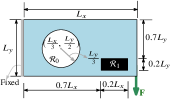
(a) Design domain

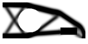
(b) $\texttt{ft=1},\,C=163.29$

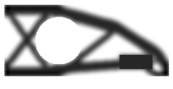
(c) $\texttt{ft=2},\,C=207.29$

Figure 11: A design domain with non-design solid and void regions is displayed in (11(a)). The optimized design with ft=1 and ft=2 are shown in (11(b)) and (11(c)) respectively.

The presented 90-line MATLAB code is modified as follows to accommodate the problem displayed in Fig. 11(a). The load vector and boundary conditions lines are changed to

⬇

F = sparse(2*(2*HNex+1),1,-1,2*Nnode,1); % Input force,

and

⬇

fixeddofs = [2*(1:2*HNex+1:(2*HNex+1)*HNey+1)-1,2*(1:2*HNex+1:(2*HNex+1)*HNey+1)]; % Fixed DOFs

respectively. An array $\mathtt{RSoVo}$ that contains information about FEs associated to the regions $\mathcal{R}_{1}$ and $\mathcal{R}_{0}$ (Fig. 11) is first initialized to $\mathtt{zeros(Nelem,1)}$ and then modified to -1 and 1 as per void and solid FEs respectively. This is performed between lines 48-49 as

⬇

if(sqrt((ct(j,1)-max(ct(:,1))/3).^2+((ct(j,2)-max(ct(:,2))/2).^2))<max(ct(:,2))/3)

RSoVo(j) = -1; % Non-design void region

end

if(ct(j,1)>0.7*max(ct(:,1))&&ct(j,1)<0.9*max(ct(:,1))&&ct(j,2)>0.1*max(ct(:,2))&&ct(j,2)<0.3*max(ct(:,2)))

RSoVo(j) = 1; % Non-design solid region

end

FEs with either -1 or 1 value in RSoVo remains passive during optimization, i.e., their material definition do not change with optimization evolution. The remnant elements with 0 indices in $\mathtt{RSoVo}$ act as active elements which decide the optimized material layout. To determine the active elements that are stored in the vector act, we introduce the following code after line 52

⬇

[NVe, NSe]= deal(find(RSoVo==-1),find(RSoVo==1));

act = setdiff((1:Nelem)’, union(NVe, NSe));

where NVe and NSe indicate arrays of FEs associated with regions $\mathcal{R}_{0}$ and $\mathcal{R}_{1}$ respectively. The design variables associated to act are provided initial values as

⬇

x(act) = (volfrac*(Nelem-length(NSe))-length(NVe))/length(act);

The sensitivities of the objective and constraints with respect to the passive design variables are zero. Therefore, while performing optimization, the active sensitivities are taken on line 77. To account non-design domains, after density filtering, the following code on line 84 is added

⬇

xPhys(RSoVo==1) = 1; xPhys(RSoVo==-1) = 0;

The 90-line code is called with above modifications as

⬇

HoneyTop90(200,100,0.4,3,6.4*sqrt(3),ft);

which gives the optimized designs displayed in Fig. 11(b) and Fig. 11(c) using ft=1 and ft=2 respectively. One can note that the optimized designs have same topologies. The design obtained with ft=2 is better than that obtained with ft=3 as the former has less objective value $C$ than the that of the latter.

4.4 Heaviside projection filter

The Heaviside projection filter is typically employed to achieve optimized solutions close to black-and-white (0-1) (Wang et al., 2011). When a Heaviside projection filter is employed, element $j$ can be characterized via three fields–(i) design variable $\rho_{j}$, (ii) filtered variable $\tilde{\rho_{j}}$ (6), and (iii) Heaviside projected variable $\bar{\rho_{j}}$ (14). The latter is termed physical variable herein and that is defined in terms of a filtered variable $\tilde{\rho_{j}}$ as (Wang et al., 2011)

$$\bar{\rho_{j}}=\frac{\tanh{\left(\beta\eta\right)}+\tanh{\left(\beta(\tilde{\rho_{j}}-\eta)\right)}}{\tanh{\left(\beta\eta\right)}+\tanh{\left(\beta(1-\eta)\right)}},$$ (14)

where $\eta\in[0,\,1]$ indicates the threshold of the filter, whereas $\beta\in[0,\,\infty)$ controls its steepness. Typically, $\beta$ is increased from $\beta_{\text{in}}=1$ to a specified maximum value $\beta_{\text{u}}$ in a continuation manner. Herein, $\beta_{\text{u}}$ is set to 128 and $\beta$ is doubled at each 60 iterations of the optimization. The derivative of $\bar{\rho_{j}}$ with respect to $\tilde{\rho_{j}}$ is

$$\frac{\partial\bar{\rho_{j}}}{\partial\tilde{\rho_{j}}}=\beta\frac{1-\tanh(\beta(\tilde{\rho_{j}}-\eta))^{2}}{\tanh{\left(\beta\eta\right)}+\tanh{\left(\beta(1-\eta)\right)}},$$ (15)

and one finds derivative of $\bar{\rho_{j}}$ with respect to ${\rho_{j}}$ using the chain rule (Wang et al., 2011) and thus, derivatives of the objective and constraints.

To accommodate this filter, the code is modified as follows. ft=3 is used to indicate the Heaviside projection filtering steps and move is set to 0.1. Note that in certain cases one may have to use continuation on the move limit to control the fluctuation of the optimization process. Before the optimization loop, the following code is added

⬇

beta = 1;

eta = 0.5;

if (ft==0|| ft == 1 || ft == 2)

xPhys = x;

elseif (ft == 3)

xTilde = x; % xTilde represents filtered variables

xPhys = (tanh(beta*eta)+tanh(beta*(xTilde-eta)))./(tanh(beta*eta)+tanh(beta*(1-eta)));

end

To evaluate the sensitivities of objective and volume constraints these lines are introduced between lines 72-73

⬇

elseif ft==3

dH= beta*(1-tanh(beta*(xTilde-eta)).^2)./(tanh(beta*eta)+tanh(beta*(1-eta)));

dc = HHs’*(dc.*dH);

dv = HHs’*(dv.*dH);

where vector dH contains $\frac{\partial\bar{\rho_{j}}}{\partial\tilde{\rho_{j}}}$ (15). Inside the optimization loop, between lines 81-82, we write the following

⬇

elseif ft == 3

xTilde = HHs’*x;

xPhys = (tanh(beta*eta)+tanh(beta*(xTilde-eta)))./(tanh(beta*eta)+tanh(beta*(1-eta)));

and the resource constraint is employed using xPhys. $\beta$ is updated in the end, between lines 89-90 as

⬇

if(ft == 3 && mod(loop,60)==0 && beta<betamax)

beta = 2*beta;

end

HoneyTop90 is called with the Heaviside projection filter for the MBB beam design (Fig. 1). We use the same parameters that are employed in Sec. 3.4. For high $\beta$, sensitivity (15) tends to zero i.e. the filtered dv tends to zero and thus, OcC (line 77) becomes unbounded. Therefore, the limits on Lagrange multiplier is set to $[0,\,10^{9}]$ i.e. a constant range, to avoid numerical instabilities as $\beta$ increases. The results are displayed in Fig. 12 with corresponding compliance values. The obtained optimized designs contain significantly negligible number of gray elements.

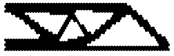
(a) $C=277.72$

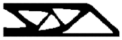
(b) $C=272.29$

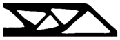
(c) $C=263.10$

Figure 12: Optimized results using HoneyTop90 with Heaviside projection filter for the MBB beam design (Fig. 1). Hexagonal elements used for (12(a)), (12(b)), and (12(c)) are $60\times 20$, $150\times 50$ and $300\times 100$, respectively.

4.5 Efficiency

In this section, the computational cost involved in evaluating each major section of HoneyTop90 is presented, and its overall runtime is compared with that of the 88-line code, top88 (Andreassen et al., 2011). The MBB beam design (Fig. 1) is solved for these studies. The filter radius and the volume fraction are set to $0.03$ times the length of the beam domain and 0.50 respectively. The SIMP penalty parameter $p$ (1) is set to 3. Codes (HoneyTop90 and top88) are run for 100 optimization iterations with ft=2 in MATLAB 2021a on a 64-bit operating system machine with 8.0 GB RAM, Intel(R), Core(TM) i5-8265U CPU 1.60 GHz.

The breakdown of the runtime of HoneyTop90 is depicted in Table 2 for different mesh sizes. Honeycomb tessellation meshgrid information and matrices for filtering are evaluated only once for one call of HoneyTop90. for loop is used to determine filter matrices in HoneyTop90 (line 45), therefore filter preparation time increases as mesh size grows. One can note that the meshgrid generation requires relatively negligible time (Table 2). FEA and optimization time increase as the mesh size increases, which is obvious.

Table 3 displays the total runtime of HoneyTop90 and top88 for 100 optimization iterations. We can note that HoneyTop90 performs faster than top88 for higher mesh sizes. In top88, volume constraint is applied using the physical design variables (filtered designs) which are evaluated at every bisection iteration inside the optimization loop by multiplying the actual design variables to the filtering matrices whose size increase as mesh size grows. However, HoneyTop90 exploits the volume preserving nature of the density filter (Wang et al., 2011) while imposing the volume constraint and thus, reduces the overall runtime. Note also that HoneyTop90 solves approximately double degrees of freedom (DOFs) system to determine the displacement vector than what top88 solves for the same mesh size (Table 3), and takes overall less runtime for larger mesh sizes.

Table 2: Breakdown of the computation time of HoneyTop90 for 100 optimization iterations

Mesh size	$60\times 20$	$180\times 60$	$300\times 100$	$420\times 140$	$480\times 160$	$600\times 200$
Meshgrid generation	0.0047 (0.089%)	0.0063 (0.024%)	0.013 (0.017%)	0.026 (0.013%)	0.041 (0.015%)	0.052 (0.009%)
Filter preparation	0.02 (0.38%)	1.189 (4.65%)	6.38 (8.2%)	26.31 (13.17%)	37.04 (13.06%)	122.16 (21.55%)
FEA + OC	1.73 (32.58%)	19.08 (74.70%)	60.01 (77.13%)	154.31 (77.29%)	215.90 (76.12%)	390.736 (68.92%)
Plotting the solutions	3.57 (67.23%)	5.28 (20.67%)	10.41 (13.38%)	19.01 (9.53%)	30.67 (10.81%)	54.1 (9.54%)
Total time of HoneyTop90	5.31	25.54	77.80	199.63	283.61	566.96

Table 3: Computation time (in seconds) required by HoneyTop90 and top88 for 100 optimization iterations. Texts in bold indicate the lower computation time for the used mesh size.

Mesh size	$60\times 20$	$180\times 60$	$300\times 100$	$420\times 140$	$480\times 160$	$600\times 200$
Total DOFs for HoneyTop90	5080	44040	121400	237160	309440	482800
Total DOFs for top88	2562	22082	60802	118722	154882	241602
Total time of HoneyTop90	5.31	25.54	77.80	199.63	283.61	566.96
Total time of top88	3.87	15.92	62.35	201.67	337.38	805.59

4.6 Other extensions

The presented code can readily be extended for different set of design problems, e.g., compliant mechanisms (Sigmund, 1997), including heat conduction (Wang et al., 2011), with design-dependent loads (Kumar et al., 2020; Kumar, 2022), etc. One can also extend the code for the problems involving multi-physics with and without many constraints and use the Method of Moving Asymptotes (MMA) (Svanberg, 1987) as an optimizer. Extension to 3D, however, is not so straightforward, one needs to employ tetra-kai-decahedron elements (Saxena, 2011) and thus, connectivity matrix and corresponding nodal coordinates are required to be generated.

5 Closure

This paper presents a simple, compact and efficient MATLAB code using hexagonal elements for topology optimization. The code is expected to ease the learning curve for a newcomer towards topology optimization with honeycomb tessellation. Due to nonsingular connectivity between neighboring elements, checkerboard patterns and point connections are circumvented inherently. However, thin members are present in the optimized designs which are noticed mesh dependent. Therefore, to circumvent mesh dependence nature of hexagonal FEs in TO, one requires to use filtering techniques or other suppressing approaches.

A novel honeycomb tessellation generation approach is presented. The code generates meshgrid information, i.e., the element connectivity matrix and nodal coordinates array for the millions of hexagonal elements within a fraction of a second using the MATLAB inbuilt functions. The element connectivity matrix and corresponding nodal coordinates generation require just 5(7) and 4(6) lines. Wachpress shape functions are employed to evaluate the stiffness matrix of a hexagonal element. The optimality criteria approach is employed for the compliance minimization problems. The provided MATLAB code (Appendix A) and its extensions are explained in detail. Easy and efficient meshgrid generation for tetra-kai-decahedron elements, performing finite element analysis and optimization form a future direction for a three-dimensional problem setting. In addition, extensions of code to solve advanced design problems with stress and buckling constraints may be one of the prime directions for future work.

Conflicts of interest

None.

Appendix A HoneyTop90 MATLAB code

⬇

1function HoneyTop90(HNex,HNey,volfrac,penal,rfill,ft)

2%% ---------- Material properties ----------

3E0 = 1;

4Emin = E0*1e-9;

5%% ---Element connectivity, nodal coordinates, Finite element analysis preparation--

6NstartVs = reshape(1:(1+2*HNex)*(1+HNey),1+2*HNex,1+HNey);

7DOFstartVs = reshape(2*NstartVs(1:end-1,1:end-1)-1,2*HNex*HNey,1);

8NodeDOFs = repmat(DOFstartVs,1,8) + repmat([2*(2*HNex+1) + [2 3 0 1] 0 1 2 3 ],2*HNex*HNey,1);

9ActualDOFs = NodeDOFs(setdiff(1:2*HNex*HNey,(2*HNex:2*HNex:2*HNex*HNey)’ + mod(1:HNey,2)’),:);

10HoneyDOFs = [ActualDOFs(2:2:end,1:2), ActualDOFs(1:2:end,:), ActualDOFs(2:2:end,7:8)];

11Ncyi = repmat(reshape(repmat([-0.25 0.25]’,HNey+1,1),2,HNey+1)+reshape(1.5*sort(repmat((0:HNey)’,2,1)),2,(HNey+1)),HNex+1,1);

12Ncyi(:,1:2:end) = flip(Ncyi(:,1:2:end));

13Ncyf = Ncyi(1:end-1,:); % final arrays containing y-coordinates

14HoneyNCO=(1)*[repmat((0:cos(pi/6):2*HNex*cos(pi/6)),1,HNey+1)’ Ncyf(:)];%node co

15if(mod(HNey,2)==0)

16 HoneyDOFs(end:-1:end-(HNex)+2,1:6) = HoneyDOFs(end:-1:end-(HNex)+2,1:6)-2; % Updating

17 HoneyNCO([(2*HNex+1)*HNey+1;(2*HNex+1)*(HNey+1)],:) = []; % Removing hangining nodes

18end

19[Nelem,Nnode] = deal(size(HoneyDOFs,1),size(HoneyNCO,1)); % elem #, node #

20 F = sparse(2*((2*HNex+1)*HNey+1),1,-1,2*Nnode,1); % Applied load

21 U = zeros(2*Nnode,1); % Initializing U

22 fixeddofs = [2*(1:2*HNex+1:(2*HNex+1)*HNey+1)-1,(2*(2*HNex+1))]; % Fixed DOFs

23 alldofs = 1:2*Nnode; % Total DOFs

24 freedofs = setdiff(alldofs,fixeddofs); % Free DOFs

25 iK = reshape(kron(HoneyDOFs,ones(12,1))’,144*Nelem,1);

26 jK = reshape(kron(HoneyDOFs,ones(1,12))’,144*Nelem,1);

27 KE = E0*[616.43012 92.77147 -168.07333 65.54377 -232.28511 -0.00032 -120.65312 -83.28564 -71.60020 -92.77115 -23.81836 17.74187;

28 92.77147 509.30685 101.02751 -71.90335 0.00032 -18.03857 -83.28564 -24.48314 -92.77179 -178.72347 -17.74187 -216.15832;

29-168.07333 101.02751 455.74522 0.00000 -168.07333 -101.02751 -71.60020 -92.77179 23.60185 -0.00000 -71.60020 92.77179;

3065.54377 -71.90335 0.00000 669.99176 -65.54377 -71.90335 -92.77115 -178.72347 -0.00000 -168.73811 92.77115 -178.72347;

31-232.28511 0.00032 -168.07333 -65.54377 616.43012 -92.77147 -23.81836 -17.74187 -71.60020 92.77115 -120.65312 83.28564;

32-0.00032 -18.03857 -101.02751 -71.90335 -92.77147 509.30685 17.74187 -216.15832 92.77179 -178.72347 83.28564 -24.48314;

33-120.65312 -83.28564 -71.60020 -92.77115 -23.81836 17.74187 616.43012 92.77147 -168.07333 65.54377 -232.28511 -0.00032;

34-83.28564 -24.48314 -92.77179 -178.72347 -17.74187 -216.15832 92.77147 509.30685 101.02751 -71.90335 0.00032 -18.03857;

35-71.60020 -92.77179 23.60185 -0.00000 -71.60020 92.77179 -168.07333 101.02751 455.74522 0.00000 -168.07333 -101.02751;

36-92.77115 -178.72347 -0.00000 -168.73811 92.77115 -178.72347 65.54377 -71.90335 0.00000 669.99176 -65.54377 -71.90335;

37-23.81836 -17.74187 -71.60020 92.77115 -120.65312 83.28564 -232.28511 0.00032 -168.07333 -65.54377 616.43012 -92.77147;

3817.74187 -216.15832 92.77179 -178.72347 83.28564 -24.48314 -0.00032 -18.03857 -101.02751 -71.90335 -92.77147 509.30685;]/1000;% elem stiffness

39%% ---------- Filter preperation ---------

40Cxx = repmat([sqrt(3)/2*(1:2:2*HNex-1) sqrt(3)*(1:1:HNex-1)],1,ceil(HNey/2));

41Cyy= (repmat(3/4,HNex,HNey) + repmat(3/2*(0:HNey-1),HNex,1));

42Cyy(HNex+1:2*HNex:length(Cyy(:))) = [];

43ct = [Cxx(1:length(Cyy))’ Cyy’]*(1); % Centre coordinates

44DD = cell(Nelem,1); % Initializing

45for j = 1:Nelem

46 Cent_dist = sqrt((ct(j,1)-ct(:,1)).^2+((ct(j,2)-ct(:,2)).^2));

47 [I,J] = find(Cent_dist<=rfill);

48 DD{j} = [I,J+(j-1),Cent_dist(I)];

49end

50 DD = cell2mat(DD);

51 HHs = sparse(DD(:,2),DD(:,1),1-DD(:,3)/rfill);

52 HHs = spdiags(1./sum(HHs,2),0,Nelem,Nelem)*HHs;

53%% ---------- Initialization -------------

54x = volfrac*ones(Nelem,1); % Initial guess

55[xPhys,loop,change,maxiter,dv,move] = deal(x,0,1,200,ones(Nelem,1),0.2); % Parameters

56%% ---------- Start optimization ----------

57while (change > 0.01 && loop < maxiter)

58 loop = loop + 1;

59 %% ---------- Finite element analysis ----------

60 sK = reshape(KE(:)*(Emin + xPhys’.^penal*(E0-Emin)),144*Nelem,1);

61 K = sparse(iK,jK,sK); % Global stiffness

62 U(freedofs) = decomposition(K(freedofs,freedofs),’chol’,’lower’)\F(freedofs);

63 %% ---------- Objective and sensitivities evaluation ----------

64 ce = sum((U(HoneyDOFs)*KE).*U(HoneyDOFs),2);

65 c = sum(sum((Emin+xPhys.^penal*(E0-Emin)).*ce)); % Finding objective

66 dc = -penal*(E0-Emin)*xPhys.^(penal-1).*ce; % Obj. sensitivities

67 %% ---------- Using Filters ---------------------------

68 if ft == 1

69 dc = HHs’*(x.*dc)./max(1e-3,x);

70 elseif ft == 2

71 dc = HHs’*(dc);

72 dv = HHs’*(dv);

73 end

74 %% ---------- Optimality criteria update ----------------

75 xOpt = x;

76 [xUpp, xLow] = deal (xOpt + move, xOpt - move); % Upp. & low. limits

77 OcC = xOpt.*(sqrt(-dc./dv)); % Opt. parameter

78 inL = [0, mean(OcC)/volfrac]; % Lag. Mul. range

79 while (inL(2)-inL(1))/(inL(2)+inL(1))> 1e-3

80 lmid = 0.5*(inL(2)+ inL(1));

81 x = max(0,max(xLow,min(1,min(xUpp,OcC/lmid))));

82 if mean(x)>volfrac, inL(1) = lmid; else, inL(2) = lmid; end

83 end

84 if ft == 1 || ft ==0, xPhys = x; elseif ft == 2, xPhys = HHs’*x; end

85 change = max(abs(xOpt-x));

86 %% ---------- Results printing ----------------------------

87 fprintf(’ It.:%5i Obj.:%11.4f Vol.:%7.3f ch.:%7.3f\n’,loop,c, mean(xPhys),change);

88 %% ---------- Plotting intermediate designs ---------------

89 colormap(’gray’); scatter(ct(:,1),ct(:,2),[],1-xPhys,’filled’); axis off equal; pause(1e-6);

90end

Appendix B Sensitivity analysis

In this paper, the optimality criteria approach is employed for the optimization. Therefore, derivatives of the objective and constraint with respect to the design variables are required. Herein, the adjoint-variable method is used to determine the sensitivity of the objective, $C({\bm{\rho}})=\mathbf{u}^{\top}\mathbf{K}(\bm{\rho})\mathbf{u}$. The overall performance function $\mathcal{L}$ in conjunction with the state equation, $\mathbf{K}\mathbf{u}-\mathbf{F}=\mathbf{0}$ is written as

$$\mathcal{L}=C+\bm{\lambda}^{\top}(\mathbf{K}\mathbf{u}-\mathbf{F}),$$ (B.1)

where $\bm{\lambda}$ is the Lagrange multiplier vector. In view of (B.1), one finds derivative of $\mathcal{L}$ with respect to $\bm{\rho}$ as

$$\begin{split}\frac{\partial\mathcal{L}}{\partial\bm{\rho}}&=\frac{\partial C}{\partial\bm{\rho}}+\frac{\partial C}{\partial\mathbf{u}}\frac{\partial\mathbf{u}}{\partial\bm{\rho}}+\bm{\lambda}^{\top}\left(\frac{\partial\mathbf{K}}{\partial\bm{\rho}}\mathbf{u}+\mathbf{K}\frac{\partial\mathbf{u}}{\partial\bm{\rho}}\right)\\ &=\mathbf{u}^{\top}\frac{\partial\mathbf{K}}{\partial\bm{\rho}}\mathbf{u}+2\mathbf{u}^{\top}\mathbf{K}\frac{\partial\mathbf{u}}{\partial\bm{\rho}}+\bm{\lambda}^{\top}\frac{\partial\mathbf{K}}{\partial\bm{\rho}}\mathbf{u}+\bm{\lambda}^{\top}\mathbf{K}\frac{\partial\mathbf{u}}{\partial\bm{\rho}}\qquad\left(\text{using},\,C({\bm{\rho}})=\mathbf{u}^{\top}\mathbf{K}(\bm{\rho})\mathbf{u}\right)\\ &=\mathbf{u}^{\top}\frac{\partial\mathbf{K}}{\partial\bm{\rho}}\mathbf{u}+\bm{\lambda}^{\top}\frac{\partial\mathbf{K}}{\partial\bm{\rho}}\mathbf{u}+\underbrace{\left(2\mathbf{u}^{\top}\mathbf{K}+\bm{\lambda}^{\top}\mathbf{K}\right)}_{\Theta}\frac{\partial\mathbf{u}}{\partial\bm{\rho}}\end{split}$$ (B.2)

In (B.2), $\Theta=0$, the adjoint equation, yields $\bm{\lambda}=-2\mathbf{u}$ and thus, one writes (B.1) as

$$\begin{split}\frac{\partial\mathcal{L}}{\partial\bm{\rho}}&=\mathbf{u}^{\top}\frac{\partial\mathbf{K}}{\partial\bm{\rho}}\mathbf{u}-2\mathbf{u}^{\top}\frac{\partial\mathbf{K}}{\partial\bm{\rho}}\mathbf{u}\\ &=-\mathbf{u}^{\top}\frac{\partial\mathbf{K}}{\partial\bm{\rho}}\mathbf{u}\end{split}$$ (B.3)

Therefore, in view of (B.3), the derivative of objective $C$ with respect to design variable $\rho_{j}$ can be written as

$$\frac{\partial C}{\partial\rho_{j}}=-\mathbf{u}_{j}^{\top}\frac{\partial\mathbf{k}_{j}}{\partial\rho_{j}}\mathbf{u}_{j}$$ (B.4)

where $\mathbf{u}_{j}$ and $\mathbf{k}_{j}$ are the displacement vector and the stiffness matrix of element $j$, respectively.

Appendix C Wachspress shape functions

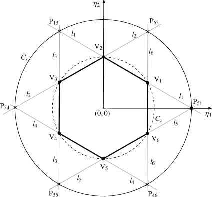
Figure C.1: A regular hexagonal element with vertices V${}_{i}|_{i=1,\,2,\,\cdots,\,6}$ and circumscribing circle ${C}_{\text{c}}$ with radius 1 unit. Coordinates of vertex V_i are $\left((\eta_{1}^{i},\,\eta_{2}^{i})\equiv\left(\cos(\frac{(2i-1)\pi}{6}),\,\sin(\frac{(2i-1)\pi}{6})\right)\right)$. Straight lines $l_{i}$ pass through vertices V_i and V_i-1. P${}_{i\,{i+2}}$ are the intersection points of straight lines $l_{i}$ and $l_{i+2}$. Circle ${C}_{\text{s}}$ with radius $\sqrt{3}$ unit is drawn that passes through points P${}_{i\,{i+2}}$.

Figure C.1 depicts a hexagonal element with vertices V${}_{i}|_{i=1,\,2,\,3,\,\cdots,\,6}$ in $\bm{\eta}$ co-ordinates system. Coordinates of vertex V_i are $\left((\eta_{1}^{i},\,\eta_{2}^{i})\equiv\left(\cos(\frac{(2i-1)\pi}{6}),\,\sin(\frac{(2i-1)\pi}{6})\right)\right)$. The circumscribing circle with radius 1 unit is represented via ${C}_{\text{c}}$. Let Wachspress shape function for vertex V_i (Fig. C.1) be $N_{i}$. Using the fundamentals of coordinate geometry and in view of coordinates of V_i, the equations of straight lines $l_{i}$ (Fig. C.1) can be written as

$$\left.\begin{aligned} l_{1}(\bm{\eta})&\equiv\eta_{1}+\sqrt{3}\eta_{2}-\sqrt{3}=0\\ l_{2}(\bm{\eta})&\equiv-\eta_{1}+\sqrt{3}\eta_{2}-\sqrt{3}=0\\ l_{3}(\bm{\eta})&\equiv 2\eta_{1}+\sqrt{3}=0\\ l_{4}(\bm{\eta})&\equiv\eta_{1}+\sqrt{3}\eta_{2}+\sqrt{3}=0\\ l_{5}(\bm{\eta})&\equiv-\eta_{1}+\sqrt{3}\eta_{2}+\sqrt{3}=0\\ l_{6}(\bm{\eta})&\equiv 2\eta_{1}-\sqrt{3}=0\end{aligned}\right\},$$ (C.1)

and likewise, the equation of circle ${C}_{\text{s}}$ (cf. Fig. C.1, passing through P_ii+2) can be written as

$${C}_{\text{s}}(\bm{\eta})\equiv\eta_{1}^{2}+\eta_{2}^{2}-3=0.$$ (C.2)

Straight lines $l_{i}$ and $l_{i+2}$ intersect at points P${}_{i\,{i+2}}$ (Fig. C.1). The shape function of node 1, i.e., $N_{1}$ is determined as (Wachspress, 1975)

$$N_{1}=s_{1}\frac{l_{2}(\bm{\eta})l_{3}(\bm{\eta})l_{4}(\bm{\eta})l_{5}(\bm{\eta})}{{C}_{\text{s}}(\bm{\eta})},$$ (C.3)

where $s_{1}$, a constant, is calculated using the Kronecker-delta property of a shape function, which is defined as

$$N_{i}(\bm{\eta}_{j})=\delta_{ij}=\left\{\begin{aligned} 1,\quad\text{if}\,\,i=j\\ 0,\quad\text{if}\,\,i\neq j\\ \end{aligned}\right..$$ (C.4)

Now, in view of coordinates of node $1$, i.e., $\left(\eta_{1}^{1},\,\eta_{2}^{1}\right)$ and (C.4), (C.3) yields

$$s_{1}=\frac{{C}_{\text{s}}(\eta_{1}^{1},\,\eta_{2}^{1})}{l_{2}(\eta_{1}^{1},\,\eta_{2}^{1})l_{3}(\eta_{1}^{1},\,\eta_{2}^{1})l_{4}(\eta_{1}^{1},\,\eta_{2}^{1})l_{5}(\eta_{1}^{1},\,\eta_{2}^{1})}=\frac{1}{18}.$$ (C.5)

Likewise, one can determine Wachspress shape functions for all other nodes with their respective constants. The final expressions of the shape functions are:

$$\left.\begin{aligned} N_{1}(\bm{\eta})&=\frac{\left(-\eta_{1}+\sqrt{3}\eta_{2}-\sqrt{3}\right)\left(2\eta_{1}+\sqrt{3}\right)\left(\eta_{1}+\sqrt{3}\eta_{2}+\sqrt{3}\right)\left(-\eta_{1}+\sqrt{3}\eta_{2}+\sqrt{3}\right)}{18\left(\eta_{1}^{2}+\eta_{2}^{2}-3\right)}\\ N_{2}(\bm{\eta})&=\frac{\left(2\eta_{1}+\sqrt{3}\right)\left(\eta_{1}+\sqrt{3}\eta_{2}+\sqrt{3}\right)\left(-\eta_{1}+\sqrt{3}\eta_{2}+\sqrt{3}\right)\left(2\eta_{1}-\sqrt{3}\right)}{18\left(\eta_{1}^{2}+\eta_{2}^{2}-3\right)}\\ N_{3}(\bm{\eta})&=-\frac{\left(\eta_{1}+\sqrt{3}\eta_{2}+\sqrt{3}\right)\left(-\eta_{1}+\sqrt{3}\eta_{2}+\sqrt{3}\right)\left(2\eta_{1}-\sqrt{3}\right)\left(\eta_{1}+\sqrt{3}\eta_{2}-\sqrt{3}\right)}{18\left(\eta_{1}^{2}+\eta_{2}^{2}-3\right)}\\ N_{4}(\bm{\eta})&=\frac{\left(-\eta_{1}+\sqrt{3}\eta_{2}+\sqrt{3}\right)\left(2\eta_{1}-\sqrt{3}\right)\left(\eta_{1}+\sqrt{3}\eta_{2}-\sqrt{3}\right)\left(-\eta_{1}+\sqrt{3}\eta_{2}-\sqrt{3}\right)}{18\left(\eta_{1}^{2}+\eta_{2}^{2}-3\right)}\\ N_{5}(\bm{\eta})&=\frac{\left(2\eta_{1}-\sqrt{3}\right)\left(\eta_{1}+\sqrt{3}\eta_{2}-\sqrt{3}\right)\left(-\eta_{1}+\sqrt{3}\eta_{2}-\sqrt{3}\right)\left(2\eta_{1}+\sqrt{3}\right)}{18\left(\eta_{1}^{2}+\eta_{2}^{2}-3\right)}\\ N_{6}(\bm{\eta})&=-\frac{\left(\eta_{1}+\sqrt{3}\eta_{2}-\sqrt{3}\right)\left(-\eta_{1}+\sqrt{3}\eta_{2}-\sqrt{3}\right)\left(2\eta_{1}+\sqrt{3}\right)\left(\eta_{1}+\sqrt{3}\eta_{2}+\sqrt{3}\right)}{18\left(\eta_{1}^{2}+\eta_{2}^{2}-3\right)}\\ \end{aligned}\right\}.$$ (C.6)

Appendix D Numerical Integration

To evaluate stiffness matrix of an element, numerical integration approach using the quadrature points is employed. As per (Lyness and Monegato, 1977), quadrature points for a hexagonal element are given in Table 4 (Saxena and Sauer, 2013), and a function $f\left(\eta_{1},\,\eta_{2}\right)$ can be integrated as

$$\int_{A_{6}}f\left(\eta_{1},\,\eta_{2}\right)\text{d}\Omega\approx A_{6}\left(w_{o}f(0,\,0)+\sum_{k=2}^{k_{\text{max}}}\sum_{i=1}^{6}w_{k}f\left(r_{k},\,\alpha_{k}+\frac{\pi i}{3}\right)\right).$$ (D.1)

where $A_{6}$ is the area of a regular hexagonal element. Table 4 notes the quadrature points $N$ with coordinates $\left(\eta_{1}^{a},\,\eta_{2}^{a}\right)$ $=\left(r_{k}\cos(\alpha_{k}+\frac{i\pi}{3}),r_{k}\sin(\alpha_{k}+\frac{i\pi}{3})\right)$. $w_{k}$ indicate the weights for these points. $i=1,\,2,\,3,\,\cdots,\,6$, if $k>1$, and $i=1,\,\text{if}\,k=1$, corresponds to single integration point at center $(0,\,0)$. For $k>1$, six integration points lie on the a circle with center at (0, 0) and radius $r_{k}$. Note that the quadrature rule is invariant under a rotation of $60^{o}$ for a hexagonal element.

Table 4: Quadrature points for a hexagonal element

Cases	$r_{k}$	$\alpha_{k}$	$w_{k}$
$1$,  $k=2$,  $N=1+6(k-1)=7$	$0.0000$	$0.0000$	$0.255952380952381$
	$0.748331477354788$	$0.0000$	0.124007936507936
$2$,  $k=3$,  $N=1+6(k-1)=13$	0.0000	$0.0000$	$0.174588684325077$
	$0.657671808727194$	$0.0000$	$0.115855303626943$
	$0.943650632725263$	$0.523681372148045$	$0.021713248985544$
$3$,  $k=4$,  $N=1+6(k-1)=19$	0.0000	$0.0000$	$0.110826547228661$
	$0.792824967172091$	$0.0000$	$0.037749166510143$
	$0.537790663359878$	$0.523598775598299$	$0.082419705350590$
	$0.883544457934942$	$0.523598775598299$	$0.028026703601157$
$4$,  $k=5$,  $N=1+6(k-1)=25$	$0.0000$	$0.0000$	$0.087005549094808$
	$0.487786213872069$	$0.0000$	$0.071957468118574$
	$0.820741657108524$	$0.0000$	$0.027500185650866$
	$0.771806696813652$	$0.523598775598299$	$0.045248932131663$
	$0.957912268790000$	$0.523598775598299$	$0.007459892497607$

References

- Andreassen et al. (2011) Andreassen E, Clausen A, Schevenels M, Lazarov BS, Sigmund O (2011) Efficient topology optimization in matlab using 88 lines of code. Structural and Multidisciplinary Optimization 43(1):1–16
- Bourdin (2001) Bourdin B (2001) Filters in topology optimization. International journal for numerical methods in engineering 50(9):2143–2158
- Bruns and Tortorelli (2001) Bruns TE, Tortorelli DA (2001) Topology optimization of non-linear elastic structures and compliant mechanisms. Computer methods in applied mechanics and engineering 190(26-27):3443–3459
- Challis (2010) Challis VJ (2010) A discrete level-set topology optimization code written in matlab. Structural and multidisciplinary optimization 41(3):453–464
- Ferrari and Sigmund (2020) Ferrari F, Sigmund O (2020) A new generation 99 line matlab code for compliance topology optimization and its extension to 3D. Structural and Multidisciplinary Optimization 62(4):2211–2228
- Giraldo-Londoño and Paulino (2021) Giraldo-Londoño O, Paulino GH (2021) Polystress: a matlab implementation for local stress-constrained topology optimization using the augmented lagrangian method. Structural and Multidisciplinary Optimization 63(4):2065–2097
- Haber et al. (1996) Haber RB, Jog CS, Bendsøe MP (1996) A new approach to variable-topology shape design using a constraint on perimeter. Structural optimization 11(1):1–12
- Han et al. (2021a) Han Y, Xu B, Liu Y (2021a) An efficient 137-line matlab code for geometrically nonlinear topology optimization using bi-directional evolutionary structural optimization method. Structural and Multidisciplinary Optimization 63(5):2571–2588
- Han et al. (2021b) Han Y, Xu B, Wang Q, Liu Y, Duan Z (2021b) Topology optimization of material nonlinear continuum structures under stress constraints. Computer Methods in Applied Mechanics and Engineering 378:113731
- Huang and Xie (2010) Huang X, Xie M (2010) Evolutionary topology optimization of continuum structures: methods and applications. John Wiley & Sons
- Kumar (2017) Kumar P (2017) Synthesis of large deformable contact-aided compliant mechanisms using hexagonal cells and negative circular masks. PhD thesis, Indian Institute of Technology Kanpur
- Kumar (2022) Kumar P (2022) Topology optimization of stiff structures under self-weight for given volume using a smooth heaviside function. Structural and Multidisciplinary Optimization 65(4)
- Kumar and Saxena (2015) Kumar P, Saxena A (2015) On topology optimization with embedded boundary resolution and smoothing. Structural and Multidisciplinary Optimization 52(6):1135–1159
- Kumar et al. (2016) Kumar P, Sauer RA, Saxena A (2016) Synthesis of c0 path-generating contact-aided compliant mechanisms using the material mask overlay method. Journal of Mechanical Design 138(6)
- Kumar et al. (2017) Kumar P, Saxena A, Sauer RA (2017) Implementation of self contact in path generating compliant mechanisms. In: Microactuators and Micromechanisms, Springer, pp 251–261
- Kumar et al. (2019) Kumar P, Saxena A, Sauer RA (2019) Computational synthesis of large deformation compliant mechanisms undergoing self and mutual contact. Journal of Mechanical Design 141(1)
- Kumar et al. (2020) Kumar P, Frouws J, Langelaar M (2020) Topology optimization of fluidic pressure-loaded structures and compliant mechanisms using the Darcy method. Structural and Multidisciplinary Optimization 61(4):1637–1655
- Kumar et al. (2021) Kumar P, Sauer RA, Saxena A (2021) On topology optimization of large deformation contact-aided shape morphing compliant mechanisms. Mechanism and Machine Theory 156:104135
- Langelaar (2007) Langelaar M (2007) The use of convex uniform honeycomb tessellations in structural topology optimization. In: 7th world congress on structural and multidisciplinary optimization, Seoul, South Korea, pp 21–25
- Lyness and Monegato (1977) Lyness J, Monegato G (1977) Quadrature rules for regions having regular hexagonal symmetry. SIAM Journal on Numerical Analysis 14(2):283–295
- Picelli et al. (2020) Picelli R, Sivapuram R, Xie YM (2020) A 101-line matlab code for topology optimization using binary variables and integer programming. Structural and Multidisciplinary Optimization pp 1–20
- Sanders et al. (2018) Sanders ED, Pereira A, Aguiló MA, Paulino GH (2018) Polymat: an efficient matlab code for multi-material topology optimization. Structural and Multidisciplinary Optimization 58(6):2727–2759
- Saxena (2011) Saxena A (2011) Topology design with negative masks using gradient search. Structural and Multidisciplinary Optimization 44(5):629–649
- Saxena and Sauer (2013) Saxena A, Sauer RA (2013) Combined gradient-stochastic optimization with negative circular masks for large deformation topologies. International Journal for Numerical Methods in Engineering 93(6):635–663
- Saxena and Saxena (2003) Saxena R, Saxena A (2003) On honeycomb parameterization for topology optimization of compliant mechanisms. In: International Design Engineering Technical Conferences and Computers and Information in Engineering Conference, vol 37009, pp 975–985
- Saxena and Saxena (2007) Saxena R, Saxena A (2007) On honeycomb representation and sigmoid material assignment in optimal topology synthesis of compliant mechanisms. Finite Elements in Analysis and Design 43(14):1082–1098
- Sigmund (1997) Sigmund O (1997) On the design of compliant mechanisms using topology optimization. Journal of Structural Mechanics 25(4):493–524
- Sigmund (2001) Sigmund O (2001) A 99 line topology optimization code written in matlab. Structural and multidisciplinary optimization 21(2):120–127
- Sigmund (2007) Sigmund O (2007) Morphology-based black and white filters for topology optimization. Structural and Multidisciplinary Optimization 33(4-5):401–424
- Sigmund and Maute (2013) Sigmund O, Maute K (2013) Topology optimization approaches. Structural and Multidisciplinary Optimization 48(6):1031–1055
- Singh et al. (2020) Singh N, Kumar P, Saxena A (2020) On topology optimization with elliptical masks and honeycomb tessellation with explicit length scale constraints. Structural and Multidisciplinary Optimization 62(3):1227–1251
- Sukumar and Tabarraei (2004) Sukumar N, Tabarraei A (2004) Conforming polygonal finite elements. International Journal for Numerical Methods in Engineering 61(12):2045–2066
- Suresh (2010) Suresh K (2010) A 199-line matlab code for pareto-optimal tracing in topology optimization. Structural and Multidisciplinary Optimization 42(5):665–679
- Svanberg (1987) Svanberg K (1987) The method of moving asymptotes–a new method for structural optimization. International journal for numerical methods in engineering 24(2):359–373
- Tabarraei and Sukumar (2006) Tabarraei A, Sukumar N (2006) Application of polygonal finite elements in linear elasticity. International Journal of Computational Methods 3(04):503–520
- Talischi et al. (2009) Talischi C, Paulino GH, Le CH (2009) Honeycomb wachspress finite elements for structural topology optimization. Structural and Multidisciplinary Optimization 37(6):569–583
- Talischi et al. (2012a) Talischi C, Paulino GH, Pereira A, Menezes IF (2012a) Polymesher: a general-purpose mesh generator for polygonal elements written in matlab. Structural and Multidisciplinary Optimization 45(3):309–328
- Talischi et al. (2012b) Talischi C, Paulino GH, Pereira A, Menezes IF (2012b) Polytop: a matlab implementation of a general topology optimization framework using unstructured polygonal finite element meshes. Structural and Multidisciplinary Optimization 45(3):329–357
- Wachspress (1975) Wachspress EL (1975) A rational finite element basis.
- Wang et al. (2021) Wang C, Zhao Z, Zhou M, Sigmund O, Zhang XS (2021) A comprehensive review of educational articles on structural and multidisciplinary optimization. Structural and Multidisciplinary Optimization 64(5):2827–2880
- Wang et al. (2011) Wang F, Lazarov BS, Sigmund O (2011) On projection methods, convergence and robust formulations in topology optimization. Structural and Multidisciplinary Optimization 43(6):767–784
- Wei et al. (2018) Wei P, Li Z, Li X, Wang MY (2018) An 88-line matlab code for the parameterized level set method based topology optimization using radial basis functions. Structural and Multidisciplinary Optimization 58(2):831–849
- Xu et al. (2020) Xu B, Han Y, Zhao L (2020) Bi-directional evolutionary topology optimization of geometrically nonlinear continuum structures with stress constraints. Applied Mathematical Modelling 80:771–791